Proposal for the detection of Majorana Fermions in Topological Superconductors

Abstract

One of the goals of modern spectroscopy is to invent techniques which detect neutral excitations that have been theoretically proposed. For superconductors, two-point transport measurements detect the Andreev crossed reflection which confirms the existence of Majorana fermions. Similar information can also be obtained from a measurement using two piezoelectric transducers. One transducer measures the stress tensor response from the strain field generated by the second transducer. The ratio between the stress response and strain velocity determines the dissipative response. We show that the dissipative stress response can be used for studying excitations in a topological superconductor. We investigate a topological superconductor for the case when an Abrikosov vortex lattice is formed. In this case the Majorana fermions are dispersive, a fact that is used to compute the dissipative stress response.

I. Introduction

The proximity of a superconductor FuKane to the surface of a topological insulator (TI) gives rise to a topological superconductor (TS) characterized by the Majorana zero modes. Recently, vortices and Majorana fermions in a magnetic field have been reported J-P.Xu in heterostructures of Bi₂Te₃/NbSe₂. Additionally, Majorana fermions have been studied in Abrikosov lattices Stern ; Franz . The Majorana zero modes are neutral excitations which, in an Abrikosov vortex lattice, become a gapless dispersive band Biswas ; Stern ; Franz . In a variety of materials a scanning tunneling microscope (STM) is used to detect charge tunneling. The spin tunneling information is usually obtained from a Magnetic Force Microscope (MFM) Hoffman ; Balatzky . Recently it was proposed that the Majorana fermions can be detected by combining STM and AFM Loss ; Yazdani ; Science .

The question which we pose here and needs to be answered is: Is it possible for a single STM measurement to detect the Majorana fermions? Two Majorana modes located at the two ends of a $p$-wave (or equivalently a one-dimensional wire with spin-orbit interaction in proximity of an $s$-wave superconductor and magnetic field) wire might be detectable by two STM experiments (two STM tips separated in space). It is important to mention that the Andreev crossed reflection Flensberg ; DavidMajorana , in which an electron is incident on one side of the superconductor and a hole comes out at the other end, has been measured in a two-leads experiment. This suggests that two STMs alone are able to detect Majorana fermions.

Here we do not discuss the two-tip experiment since it is similar to the Andreev reflection experiment, instead we consider the sound wave analog. The analogous configuration for two STMs tips can be realized by two piezoelectric transducers. One transducer is used to generate a strain wave, whereas the other is used to detect the stress response. The stress response is equivalent to the electromagnetic (paramagnetic) response of a superconductor to an electric field Schrieffer . We show here that for a TS the stress response also probes the Majorana modes.

A number of methods based on sound waves have been used to investigate superconductors Maali ; Maynard ; Aref ; Magnusson . Ultrasound attenuation studies Kadanoff ; Tsuneto , and investigations of the $p$-wave superconductor Sr₂RuO₂ have been carried out in ref. Maki . In the late fifties ultrasound attenuation techniques were used to measure the temperature dependence of the superconducting gap Tinkham ; Schrieffer ; Philip ; Rodriguez ; Tremblay and recently the techniques have been applied to liquid ³He Nagai .

The purpose of this paper is to demonstrate that piezoelectric transducers can be used to detect Majorana fermions in an Abrikosov vortex lattice. The tunneling amplitude of the Majorana fermions gives rise to a dispersive band Biswas which is detectable. We compute the stress viscosity as a response to an applied strain velocity field LandauI ; LandauII . The explicit dependence of the strain field on the system is obtained from a coordinate transformation Katanaev . The linear stress response theory Fetter used for a TS provides information about the Majorana fermions. In order to demonstrate the detection of Majorana fermions we consider a TS Ivanov ; FuKane ; Yakovenko ; J-P.Xu ; Stern ; Franz which has an Abrikosov vortex lattice.

In this paper we have derived the following specific results: (a) We have obtained the vortex lattice solution for a $p$-wave superconductor. (b) We have derived the stress-strain Hamiltonian and have computed the stress viscosity using the linear response theory. (c) We have identified the sound analog of the Andreev crossed reflection and have obtained the viscosity equivalent to the crossed reflection conductance.

The structure of the paper is as follows: In Sec. II we show that for an attractive interaction on the surface of a TI a TS is obtained. In the presence of an Abrikosov vortex lattice dispersive Majorana fermions are formed. In Sec. III we present the formation of the Abrikosov vortex lattice. We find dispersive Majorana fermions and quasi-particles in the vortex lattice. A new solution for the $p$-wave Abrikosov vortex lattice is obtained and discussed in detail. Section IV is devoted to the derivation of the viscosity tensor for a TS. In Sec.V we compare our results to the one obtained by the ultrasound attenuation technique. In Sec.VI we compute the transverse impedance for the TS in a magnetic field. The transverse impedance provides distinct information about the Abrikosov vortex lattice and the Majorana fermions. Section VII is devoted to comments on the Andreev crossed reflection induced in one dimension by a piezoelectric transducer. Section VIII contains our main conclusions.

II. Formation of Majorana fermions on the surface of a TI with attractive interactions

In this section we review the formation of a $p$-wave superconductor on the surface of a TI with attractive interactions. For two space dimensions, the quantum Hall system and the $p$-wave superconductor Ivanov ; FuKane ; Yakovenko are characterized by the first Chern integer number $C^{1}$ (which means that the integral of the Berry curvature over a closed manifold is quantized in units of $2\pi$) Taylor . In the presence of an attractive interaction (due to the electron-phonon interaction or proximity to another superconductor), on the surface of a TI a two-dimensional TS emerges. The proximity of a superconductor FuKane to the three dimensional TI gives rise to Majorana zero modes on the surface of the TI. Recently it was reported that the application of a magnetic field on the heterostructure Bi₂Te₃/NbSe₂ induces an Abrikosov vortex lattice J-P.Xu .

We propose that a realization of the model introduced in FuKane emerges from the TI surface Hamiltonian $h(\vec{k})=-\sigma_{2}k_{1}+\sigma_{1}k_{2}$ in the presence of an attractive interaction. We express the pairing interaction in terms of the field $\psi_{\sigma}(\vec{x})=\sum_{k}e^{i\vec{k}\cdot\vec{x}}u^{(+)}(\vec{k})_{\sigma}$ where $u^{(+)}(\vec{k})_{\sigma}$ are the TI surface spinors for the conduction band, $u^{(+)}(\vec{k})=\frac{1}{\sqrt{2}}\Big{[}1,i\frac{k_{1}-ik_{2}}{|\vec{k}|}|\Big{]}^{T}\approx\frac{1}{\sqrt{2}}\Big{[}1,i\frac{k_{1}-ik_{2}}{k_{0}}\Big{]}^{T}$ ($T$ stands for transpose), and $k_{0}$ is a momentum scale. This representation generates the linear derivatives of the pairing field. For a positive chemical potential $\mu>0$ in the presence of a magnetic field, it gives rise to a superconductor with vortices. The attractive interaction expressed in terms of the TI spinors gives rise to the $p$-wave Hamiltonian FuKane which in our case also includes vortices.

$$H_{T.I.+SC.}=\int\,d^{2}x\Big{[}C^{\dagger}(\vec{x})\frac{v}{2k_{F}}\Big{(}(-i\vec{\partial}_{x}-\frac{e}{\hbar}\vec{A}(\vec{x},t))^{2}-k^{2}_{F}\Big{)}C(\vec{x})+\frac{\Delta^{*}(\vec{x},t)}{2k_{0}}C(\vec{x},t)\Big{(}\partial_{1}-i\partial_{2}\Big{)}C(\vec{x},t)$$

$$-\frac{\Delta(\vec{x},t)}{2k_{0}}C^{\dagger}(\vec{x},t)\Big{(}\partial_{1}+i\partial_{2}\Big{)}C^{\dagger}(\vec{x},t)+\frac{1}{g}|\Delta(\vec{x},t)|^{2}\Big{]}.$$

The pairing field $\Delta(\vec{x})$ depends on the phase $\theta(\vec{x})$ which includes a multivalued part. We perform the gauge transformation: $C(\vec{x})=e^{\frac{-i}{2}\theta(\vec{x})}\hat{C}(\vec{x})$, $C^{\dagger}(\vec{x})=\hat{C}^{\dagger}(\vec{x})e^{\frac{i}{2}\theta(\vec{x})}$ and the Hamiltonian $H$ is replaced by $\hat{H}$. The pairing field $\Delta(\vec{x})$ has points $\vec{x}\approx\vec{R}_{k}$, $k=1,2,...$, where $\Delta(\vec{x})$ vanishes, $\Delta(\vec{x})\approx|\Delta|e^{i\theta(\vec{x})}$, $\Delta^{\dagger}(\vec{x})=|\Delta|e^{-i\theta(\vec{x})}$, where $\theta(\vec{x})\equiv\theta(\vec{x};\vec{R}_{0}=0,\vec{R}_{1},...,\vec{R}_{k},...)$ is the multivalued phase. As a result of the gauge transformation the fermion operators $C(\vec{x})$, $C^{\dagger}(\vec{x})$ are replaced by $\hat{C}^{\dagger}(\vec{x})$, $\hat{C}(\vec{x})$ (and the Hamiltonian $H$ is replaced by $\hat{H}$). The Hamiltonian $\hat{H}$ without the condensation energy $\frac{1}{g}|\Delta(\vec{x},t)|^{2}$ is expressed in terms of the particle-hole Pauli matrices $\tau_{1}$, $\tau_{2}$ and $\tau_{3}$. We introduce the two-component spinor $\hat{\Psi}(\vec{x})=\Big{[}\hat{C}(\vec{x}),\hat{C}^{\dagger}(\vec{x})\Big{]}^{T}$ and find:

$$\hat{H}=\int\,d^{2}x\hat{\Psi}^{\dagger}(\vec{x})\Big{[}\tau_{3}\hat{h}_{3}+\tau_{2}\hat{h}_{2}+\tau_{1}\hat{h}_{1}\Big{]}\hat{\Psi}(\vec{x}),\hskip 3.97432pt\frac{1}{2}\vec{\partial}_{x}\theta(\vec{x})\equiv\frac{1}{2}\sum_{l}\vec{\partial}_{x}\varphi_{l}(\vec{x}),\varphi_{l}(\vec{x})\equiv\arg\Big{(}\vec{x}-\vec{R}_{l}\Big{)},$$

$$\hat{h}_{3}=\frac{v}{2k_{F}}\Big{(}\Big{(}-i\vec{\partial}_{x}-\frac{e}{\hbar}\vec{A}(\vec{x})+\frac{1}{2}\vec{\partial}_{x}\theta(\vec{x})\Big{)}^{2}-k^{2}_{F}\Big{)},\hskip 3.97432pt\hat{h}_{2}=i\frac{|\Delta(\vec{x})|}{2k_{0}}\partial_{1},\hskip 1.8063pt\hat{h}_{1}=-i\frac{|\Delta(\vec{x})|}{2k_{0}}\partial_{2}.$$

The spinor $\hat{\Psi}(\vec{x})=\Big{[}\hat{C}(\vec{x}),\hat{C}^{\dagger}(\vec{x})\Big{]}^{T}$ Jackiw contains two parts, the non-zero mode $\hat{\Psi}_{\neq 0}(\vec{x})$ and the zero mode (Majorana fermions) $\hat{\Psi}_{0}(\vec{x})$, $\hat{\Psi}(\vec{x})\equiv\hat{\Psi}_{\neq 0}(\vec{x})+\hat{\Psi}_{0}(\vec{x})$.

III. TS Abrikosov vortex lattice

Next we discuss in detail the non-zero and zero modes of the Abrikosov lattice in a TS.

A. Non-zero modes

In this section we consider the non-zero modes for an Abrikosov vortex lattice in the presence of a magnetic field. The experimental work on the TS Bi₂Te${}_{3}/$NbSe₂ J-P.Xu shows that an Abrikosov vortex lattice is formed. A vortex lattice is stabilized for superconductors when the penetration depth of the magnetic field is larger than the coherence length Tinkham ; Abrikosov . Following Appendix A we find for a single vortex a string-like solution for the effective magnetic field. For $|\vec{\hat{x}}|>d\approx\lambda_{L}$ the magnetic field vanishes (d is the vortex lattice constant and $\lambda_{L}$ is the magnetic penetration depth). Since we are interested in the long distance behavior we can approximate the magnetic field for $|\vec{x}|<\lambda_{L}$ by a constant field, which is the spatial average around the vortex core with a radius of $d$.

Following refs. Abrikosov ; Tinkham we solve the $p$-wave Hamiltonian in a periodic magnetic field $b$. The periodicity being $d\approx\lambda_{L}$. The periodic spinor solution is given by:

$\mathbf{W(\vec{x})=\sum_{n_{2}}e^{iqn_{2}y}f_{n_{2}}(x)W(x,n_{2})}$, where $\mathbf{f_{n_{2}}(x)=e^{\frac{-b}{2}(x-\frac{q}{b}n_{2})^{2}}}$ and $\mathbf{W(x,n_{2})=\Big{[}U(x,n_{2}),V(x,n_{2})\Big{]}^{T}}$ is a two component spinor which is given by the eigenfunction of the $p$-wave Hamiltonian. We consider a square lattice and the solution is periodic in the $y$ direction with the periodicity $d=d_{y}=\frac{2\pi}{q}$. The periodicity in the $x$ direction $d=d_{x}=\frac{q}{b}$ is achieved by demanding the invariance of the Hamiltonian under the transformation, $n_{2}\rightarrow n_{2}+1$. The system has a finite extention $L$ in the $x$ direction. Therefore the value of the momentum in the $y$ direction must be restricted to $|n_{2}|<n_{max.}=\frac{bL}{q}=\frac{2L}{d}$ (to ensure that the states lie in the box $L\times L$).

Due to the spinor structure of the solution it is convenient to solve the problem in the momentum space and at the end to impose the periodicity of the wave function. We represent the periodic solution as: $\mathbf{W(\vec{x})=\int\,\frac{d^{2}k}{(2\pi)^{2}}e^{i\vec{k}\cdot\vec{x}}W(\vec{k})}$. We use the momentum representation, $x=i\partial_{k_{1}}$ and find that for the $p$-wave Hamiltonian $h(\vec{k},i\partial_{k_{1}})$ in the magnetic field $b$:

$$h(\vec{k},i\partial_{k_{1}})=\tau_{3}\frac{v}{2k_{F}}\Big{[}k^{2}_{1}+\Big{(}k_{2}+ib\partial_{k_{1}}\Big{)}^{2}-k^{2}_{F}\Big{]}+\tau_{1}\frac{\Delta}{2k_{0}}k_{2}-\tau_{2}\frac{\Delta}{2k_{0}}k_{1},$$

$$h(\vec{k},i\partial_{k_{1}})W(\vec{k})=E(\vec{k})W(\vec{k}),$$

where $bi\partial_{k_{1}}$ is the $y$ component of the vector potential in the Landau gauge for the periodic magnetic field. The eigenvectors and eigenvalues are computed next. The ground state is given in terms of the ground state energy of the Harmonic oscillator solution, $\epsilon_{0}(b,k_{F})\equiv\frac{vk_{F}}{2}\Big{(}\sqrt{\frac{b^{2}}{2}}\Big{)}$:

$$W(\vec{k})=e^{i\frac{k_{1}k_{2}}{b}}e^{-\frac{k^{2}_{1}\sqrt{2}}{b}}W(\vec{k}),$$

$$W(\vec{k})=\frac{1}{\sqrt{2}}\Big{[}e^{-i\chi(\vec{k})}\sqrt{1+\frac{\epsilon_{0}(b,k_{F})}{E(\vec{k})}},\sqrt{1-\frac{\epsilon_{0}(b,k_{F})}{E(\vec{k})}}\Big{]}^{T},$$

$$E(\vec{k})=\sqrt{\epsilon^{2}(b,k_{F})+(\frac{\Delta}{2k_{0}})^{2}(k^{2}_{1}+k^{2}_{2})},\hskip 7.22743pt\epsilon_{0}(b,k_{F})-\frac{v}{2k_{F}}k^{2}_{F}\equiv\epsilon_{0}(b,k_{F})-\frac{vk_{F}}{2}k^{2}_{F}=\frac{vk_{F}}{2}\Big{(}\frac{1}{2\pi}\frac{q^{2}}{k^{2}_{F}}-1\Big{)}.$$

We note that ${\Delta}/{2k_{0}}$ is dimensionless. At this stage we impose the periodic boundary conditions. This results in replacing $k_{1}=qn_{1}$, $k_{2}=qn_{2}$ with the condition $|n_{2}|<n_{max.}=\frac{bL}{q}=\frac{2L}{d}$, $q=\frac{2\pi}{d}$. As a result the eigenspinors and eigenvectors are given in terms of the integers $n_{1},n_{2}$:

$$W(n_{1},n_{2})=\sqrt{\frac{1}{2n_{max.}+1}}e^{i\frac{q^{2}n_{1}n_{2}}{b}}e^{-\frac{q^{2}n^{2}_{1}\sqrt{2}}{b}}\hat{\hat{W}}(n_{1},n_{2}),$$

$$W(n_{1},n_{2})=\frac{1}{\sqrt{2}}\Big{[}e^{-i\chi(n_{1},n_{2})}\sqrt{1+\frac{\epsilon(b,k_{F})}{E(n_{1},n_{2})}},\sqrt{1-\frac{\epsilon(b,k_{F})}{E(n_{1},n_{2})}}\Big{]}^{T}\equiv\Big{[}U(n_{1},n_{2}),V(n_{1},n_{2})\Big{]},$$

$$E(n_{1},n_{2})=\sqrt{\epsilon^{2}(b,k_{F})+(\frac{\Delta q}{2k_{0}})^{2}(n^{2}_{1}+n^{2}_{2})},\hskip 7.22743pt\epsilon(b,k_{F})=\epsilon(b,k_{F})\equiv\frac{vk_{F}}{2}\Big{(}\frac{q^{2}}{8\pi k^{2}_{F}}-1\Big{)}.$$

The spinor $\mathbf{W(n_{1},n_{2})}$ determines the non-zero mode fermion fields. We introduce the annihilation and creation operators $\eta(n_{1},n_{2})$, $\eta^{\dagger}(n_{1},n_{2})$ with respect to the exact ground state $|G\rangle$, $\eta(n_{1},n_{2})|G\rangle=0$ which allows us to write:

$$\hat{\Psi}_{\neq 0}(\vec{x})=\sum_{n_{1}}\sum_{n_{2}}e^{iqn_{1}x_{1}+i\frac{q}{2}n_{2}x_{2}}\Big{[}\eta(n_{1},n_{2})\mathbf{W(n_{1},n_{2})}+\eta^{\dagger}(-n_{1},-n_{2})\tau_{1}\otimes I\mathbf{W^{*}(-n_{1},-n_{2})}\Big{]},$$

$$\hat{\Psi}^{\dagger}_{\neq 0}(\vec{x})=\sum_{n_{1}}\sum_{n_{2}}e^{-iqn_{1}x_{1}-i\frac{q}{2}n_{2}x_{2}}\Big{[}\eta^{\dagger}(n_{1},n_{2})\mathbf{W^{*}(n_{1},n_{2})}+\eta(-n_{1},-n_{2})\mathbf{W(n_{1},n_{2})}\tau_{1}\otimes I\Big{]}.$$

We have replaced the discrete sites by the coordinate $x$ in order to consider even and odd rows that we need to introduce in the matrix $I$ and double the dimension of the spinor. (This needs to be done in order to have the same dimension for the zero and nonzero modes). Taking in consideration also the particle-hole symmetry we use the representation $\tau_{1}\otimes I$, which is four-dimensional; $\tau_{1}$ acts on the particle-hole space and $I=1,2$ acts on the even and odd row in real space.

B. Zero modes

In this section we consider the zero modes for an Abrikosov vortex lattice. In the absence of the vortex lattice the zero-mode solutions for the Hamiltonian in Eq. $(2)$ are given by: $W_{0}(\vec{x})\equiv W_{0}(r,\varphi)=\Big{[}U_{0}(r,\varphi),V_{0}(r,\varphi)\Big{]}^{T}\equiv\Big{[}\frac{1}{\sqrt{i}}e^{\frac{i}{2}\varphi},\frac{1}{\sqrt{-i}}e^{\frac{-i}{2}\varphi}\Big{]}^{T}\frac{F(r)}{\sqrt{r}}$ (see Appendix B) The function $\frac{F(r)}{\sqrt{r}}$ obeys the normalization condition $\int\,d^{2}r[\frac{F(r)}{\sqrt{r}}]^{2}<\infty$. Due to the charge conjugation property of the Hamiltonian, the zero modes are Majorana modes. The solution obtained here is similar to the solution given in refs. ReadI ; Taylor for the $p$-wave superconductors. The explicit form of the kinetic operator determines the exact form of the amplitude $\frac{F(r)}{\sqrt{r}}$ for the zero modes DaSarma . We consider the case where the gauged transformed Hamiltonian $\hat{H}$ has $2N$ Majorana zero modes. The Majorana operators obey $\gamma_{l}=\gamma^{\dagger}_{l}$, $\gamma^{2}_{l}=\frac{1}{2}$ for $l=1,...,2N$,

$$\hat{\Psi}_{0}(\vec{x})=\sum_{l=1}^{2N}\gamma_{l}\Big{[}\frac{1}{\sqrt{i}}e^{\frac{i}{2}\varphi_{l}(\vec{x})},\frac{1}{\sqrt{-i}}e^{\frac{-i}{2}\varphi_{l}(\vec{x})}\Big{]}^{T}\frac{F(|\vec{x}-\vec{R}_{l}|)}{\sqrt{|\vec{x}-\vec{R}_{l}|}}.$$ (7)

In the second stage we want to discuss the effect of the vortex lattice on the localized Majorana fermions. The effect of the vortex lattice is to delocalize the Majorana fermions and form dispersive Majorana bands. This is a result due to ref. Stern which showed that Majorana fermions enclose a flux which depends on the number of vortices on a closed polygon. The flux on a polygon of $n$ vortices is $\frac{\pi}{2}(n-2)$ (n is the number of vortices in the polygon) Stern . For a square vortex lattice with four vortices ($n=4$) per plaquette the flux will be $\frac{\pi}{2}(4-2)=\pi$. For the Majorana case we restrict ourselves to plaquettes with four vortices (per plaquette) Stern . We consider the effect of the overlap between Majorana fermions given by matrix element $t_{0}$ Stern ; Biswas .

$$H_{0}=it_{0}\sum_{i,j}\hat{\Psi}_{0}^{\dagger}(x_{i})S(x_{i},x_{j})\hat{\Psi}_{0}(x_{j}),$$ (8)

where $S(x_{i},x_{j})$ introduces the phase on the bond $i,j$ and determines the flux of $\pi$ per plaquette and $t_{0}$ is the overlap between the Majorana fermions which is determined from Eq. $(7)$. (The minimum energy for the Abrikosov vortices is obtained for a triangular lattice Abrikosov . For a square lattice the energy is less favorable, but it is simpler to analyze.)

We choose a gauge for which the hopping constant along columns has positive sign and alternating signs between adjacent rows. This means that $S(x_{i},x_{j})=|S(x_{i},x_{j})|e^{i\theta_{i,j}}$, the phase $\theta_{i,j}$ is zero along columns, has positive sign ($\theta_{i,j}=0$) and alternating signs between adjacent rows ($\theta_{i,j}=\pi$) Stern . As a result we obtain two flat bands and a third band that is dispersive and gapless Biswas ; Stern ; Franz comprising Majorana fermions with the eigenvalues:

$$\lambda^{0}_{\alpha=1}(\vec{k})\equiv\lambda(\vec{k})=t_{0}\sqrt{\sin^{2}(k_{1})+\sin^{2}(k_{2})},\hskip 7.22743pt|\vec{k}|\leq{\frac{\pi}{2}},\hskip 7.22743pt\lambda^{0}_{\alpha=2}(\vec{k})=0.$$ (9)

For the zero modes we find that the representation of the zero modes is given in terms of the zero mode Majorana operators in the continuum representation $\Gamma(\vec{x})=\Gamma^{\dagger}(\vec{x})$ ($x_{i}$ is replaced with the continuum coordinate $x$, even and odd rows are introduced with the help of the matrix $I$) and spinor eigenfunctions are given in momentum space $L(\vec{k})$:

$$\hat{\Psi}_{0}(\vec{x})=\sum_{k}e^{i\vec{k}\cdot\vec{x}}\Big{[}\Gamma(\vec{k})L(\vec{k})+\Gamma^{\dagger}(-\vec{k})\tau_{1}\otimes IL^{*}(-\vec{k})\Big{]},$$

$$\hat{\Psi}^{\dagger}_{0}(\vec{x})=\sum_{k}e^{-i\vec{k}\cdot\vec{x}}\Big{[}\Gamma^{\dagger}(\vec{k})L^{*}(\vec{k})+\Gamma(-\vec{k})L(-\vec{k})\tau_{1}\otimes I\Big{]}.$$

The four components of the spinor $L(\vec{k})$ in Eq. $(10)$ are given by:

$$L(\vec{k})=\frac{1}{\sqrt{2}\sqrt{\sin^{2}[k_{1}]+4(\sin[k_{1}]+\lambda(\vec{k}))^{2}}}$$

$$\Big{[}\sin[k_{2}],\sin[k_{2}],\frac{-i(\sin[k_{1}]+\lambda(\vec{k}))}{\sin[k_{2}]}(1-e^{2ik_{2}}),\frac{-i(\sin[k_{1}]+\lambda(\vec{k}))}{\sin[k_{2}]}(1-e^{2ik_{2}})\Big{]}^{T}.$$

We replace the discrete sites $x_{i}$ by the coordinate $x$, therefore we introduce the matrix $I$ to double the dimension of the spinor. Taking in consideration also the particle-hole symmetry we use the representation $\tau_{1}\otimes I$ which is four-dimensional; $\tau_{1}$ acts on the particle-hole space and $I=1,2$ acts on the even and odd row. We note that a triangular lattice for the Majorana modes has been considered in refs. Biswas ; Stern .

IV. Viscosity tensor for the TS

In the first part we introduced the theory for the dissipative viscosity and in the second part we used this theory to investigate the Abrikosov lattice. The physics of solids LandauI and fluids LandauII provides us the relation between the stress tensor $\Sigma_{i,j}$, strain field $\epsilon_{kl}$ and the velocity strain field $v_{kl}=\partial_{t}(\epsilon_{kl})$ Kosevich . We now use this description for quantum fluids in a solid. The combination of the stress tensor resulting from a strain field and the dissipative part of the stress determines the equation:

$$\Sigma_{i,j}=\lambda_{ij,kl}\epsilon_{kl}+\zeta_{ij,kl}v_{kl}.$$ (12)

The strain field $\epsilon_{k,l}$ is given in terms of the lattice deformation $\vec{u}(\vec{x},t)$, $\epsilon_{k,l}=\frac{1}{2}(\partial_{k}u^{l}+\partial_{l}u^{k})$, $\epsilon_{0,i}=\partial_{t}u^{i}$. The viscosity tensor is given by $\zeta_{ij,kl}\equiv\frac{\Sigma_{i,j}}{v_{k,l}}$, and $\zeta_{ij,kl}$ is separated into two parts, $\zeta_{ij,kl}=\zeta^{S}_{ij,kl}+\zeta^{A}_{ij,kl}$, $\zeta^{S}_{ij,kl}=\zeta^{S}_{kl,ij}$ is the symmetric part and $\zeta^{A}_{ij,kl}=-\zeta^{A}_{kl,ij}$ is the antisymmetric part Avron . From the Onsager relations Onsager we know that when the time reversal symmetry is violated, like in the quantum Hall system and the $p$-wave superconductor case Avron ; Yakovenko ; Read ; Son , we have $\zeta^{A}_{ij,kl}\neq 0$. For $\zeta_{ii,kk}$ with $i\neq k$ we have a situation where the strain field generates stress in the perpendicular direction. The stress tensor for quantum fluids is obtained from the invariance of the Lagrangian under an arbitrary local coordinate transformation Nakahara ; Katanaev ; DavidR ; DavidD . The explicit dependence of the strain field on the lattice deformation determines the coordinate transformation Katanaev from which we obtain the stress tensor. In the presence of an elastic deformation $\vec{u}$ the coordinates transform in the following way: $\vec{x}\rightarrow\vec{\xi}(\vec{x})=\vec{x}+\vec{u}(\vec{\xi})$ Katanaev (see Appendix C).

This coordinate transformation allows the identification of the stress tensor. Using the invariance of the spinless fields under the coordinate deformation gives,

$$\mathbf{\hat{C}}(\vec{\xi}(\vec{x}))=\hat{C}(\vec{x}),\hskip 10.84006pt\mathbf{\hat{C}^{\dagger}}(\vec{\xi}(\vec{x}))=\hat{C}^{\dagger}(\vec{x}).$$ (13)

For the $p$-wave Hamiltonian given in Eq. $(2)$ we find the momentum density $\pi_{i}(\vec{x},t)$ and stress tensor $\Sigma_{ij}(\vec{x},t)$ induced by the strain fields $\epsilon_{0,i}(\vec{x},t)$, $\epsilon_{i,j}(\vec{x},t)$. To linear order in the deformation strain field we obtain the response stress field. Using the invariance, Eq. $(13)$, with respect to the coordinate transformation determines the strain-stress Hamiltonian $H^{ext.}(t)$:

$$H^{ext.}(t)=\int\,d^{2}x\Big{[}\epsilon_{0,1}(\vec{x},t)\pi_{1}(\vec{x},t)+\epsilon_{0,2}(\vec{x},t)\pi_{2}(\vec{x},t)+\epsilon_{1,1}(\vec{x},t)\Sigma_{11}(\vec{x},t)+\epsilon_{22}(\vec{x},t)\Sigma_{22}(\vec{x},t)$$

$$+\epsilon_{12}(\vec{x},t)\Sigma_{12}(\vec{x},t)+\Omega_{12}(\vec{x},t)R_{12}(\vec{x},t)\Big{]}.$$

In the absence of disclinations $\Omega_{12}(\vec{x},t)=0$ in Eq. $(14)$.

Using the explicit dependence of the spinor in terms of the zero and nonzero modes given in Eqs. (5), (10) allows us to represent the stress fields:

$$\pi_{1}(\vec{x},t)=\hat{\Psi}^{\dagger}(\vec{x},t)\Big{(}Ii\partial_{1}\Big{)}\hat{\Psi}(\vec{x},t);\hskip 7.22743pt\pi_{2}(\vec{x},t)=\hat{\Psi}^{\dagger}(\vec{x},t)\Big{(}Ii\partial_{2}\Big{)}\hat{\Psi}(\vec{x},t),$$

$$\Sigma_{11}(\vec{x},t)\approx-\frac{\Delta}{2k_{0}}\hat{\Psi}^{\dagger}(\vec{x},t)\Big{(}\tau_{2}(-\partial_{1})\hat{\Psi}(\vec{x},t)\Big{)};~{}~{}\Sigma_{22}(\vec{x},t)\approx-\frac{\Delta}{2k_{0}}\hat{\Psi}^{\dagger}(\vec{x},t)\Big{(}\tau_{1}(-i\partial_{2})\Big{)}\hat{\Psi}(\vec{x},t),$$

$$\Sigma_{12}(\vec{x},t)\approx\frac{\Delta}{2k_{0}}\hat{\Psi}^{\dagger}(\vec{x},t)\Big{(}\tau_{2}(-i\partial_{2})+\tau_{1}(-i\partial_{1})\Big{)}\hat{\Psi}(\vec{x},t);$$

$$R_{12}(\vec{x},t)\approx\frac{\Delta}{2k_{0}}\hat{\Psi}^{\dagger}(\vec{x},t)\Big{(}\tau_{2}(-i\partial_{2})-\tau_{1}(-i\partial_{1})\Big{)}\hat{\Psi}(\vec{x},t);~{}~{}\hat{\Psi}(\vec{x})\equiv\hat{\Psi}_{\neq 0}(\vec{x})+\hat{\Psi}_{0}(\vec{x}).$$

We compute the viscosity stress tensor and the dissipative viscosity tensor $\zeta_{ij,kl}(\vec{q},\Omega)=\frac{\Sigma_{ij}(\vec{q},\Omega)}{v_{kl}(-\vec{q},-\Omega)}$ in quantum fluids. We vary the $p$-wave Hamiltonian by a linear strain field $\delta u^{i}(\vec{x},t)$, $u^{i}(\vec{x},t)\rightarrow u^{i}(\vec{x},t)+\delta u^{i}(\vec{x},t)$ and find from Eq. $(6)$ that the variation with respect to $\delta u^{i}(\vec{x},t)$ satisfies the continuity equation:

$$\partial_{t}\pi_{j}(\vec{x},t)+\sum_{i}\partial_{i}\Sigma_{ij}(\vec{x},t)=0.$$ (16)

Using the linear response theory Fetter with respect to the strain-stress Hamiltonian $H^{ext.}(t)$ given in Eq. $(14)$ we obtain:

$$\langle G|\Sigma_{ij}(x,t)|G\rangle_{ext.}=\langle G|\Sigma_{ij}(x,t)|G\rangle+(\frac{-i}{\hbar})\int_{0}^{t}\,dt^{\prime}\langle G|[\Sigma^{H}_{ij}(x,t),H_{H}^{ext.}(t^{\prime})]|G\rangle,$$ (17)

where $\Sigma^{H}_{ij}(x,t)$ is the stress in the Heisenberg representation with the ground state $|G\rangle$ given in Eqs. (6), (11). Following ref. Fetter we obtain the relation $\Sigma_{ij}(\vec{q},\Omega)=\zeta_{ij,kl}(\vec{q},\Omega)v_{kl}(-\vec{q},-\Omega)$:

$$R_{ij,kl}(\vec{q},t)=(\frac{-i}{\hbar})\langle G|\mathbf{T}\Big{(}\Sigma_{ij}(\vec{q},t)\Sigma_{kl}(-\vec{q},0)\Big{)}|G\rangle,~{}~{}R_{ij,kl}(\vec{q},\Omega)=\int_{-\infty}^{\infty}R_{ij,kl}(\vec{q},t)e^{-i\Omega t}\,dt,$$

$$\zeta_{ij,kl}(\vec{q},\Omega)=-\frac{R_{ij,kl}(\vec{q},\Omega)}{i\Omega}.$$

The dissipative $\zeta_{ij,kl}(\vec{q},\Omega)$ part of the viscosity tensor is obtained after the analytic continuation $i\Omega\rightarrow\Omega+i0^{+}$. Equation $(18)$ is computed using Wick’s theorem Fetter for the stress $\Sigma_{ij}(\vec{q},t)$ which is expressed in terms of the spinor $\hat{\Psi}_{(}\vec{x})=\hat{\Psi}_{\neq 0}(\vec{x})+\hat{\Psi}_{0}(\vec{x})$ in Eq. $(15)$.

V. Application of the viscosity tensor to ultrasound attenuation

In this section we compare our calculation to the existing ultrasound attenuation method given in the literature Tinkham ; Schrieffer ; Philip . For the topological superconductors we need to work with the spinor $\hat{\Psi}(\vec{x})=\hat{\Psi}_{\neq 0}(\vec{x})+\hat{\Psi}_{0}(\vec{x})$. Due to the dispersive nature of the zero modes, we will have new contributions to the absorption from the mixed pairs $\hat{\Psi}_{\neq 0}(\vec{x})$ and $\hat{\Psi}_{0}(\vec{x})$.

In a superconductor the electron-phonon interaction couples to longitudinal as well as transverse phonons. The coupling of the electrons to the transverse phonons in the superconducting phase is less understood. We show that by applying a transverse strain we can obtain non-diagonal response for stress; in this way we study the transverse effect of phonons.

The ultrasound attenuation method measures the superconducting gap. The single particle contribution to the absorption in a superconductor is given by $\frac{\alpha_{sc}}{\alpha_{normal}}=\frac{2}{e^{\frac{\Delta(T)}{T}}+1}$ ($\alpha_{sc}$ is the absorption for the superconductor and $\alpha_{normal}$ is the absorption in the normal phase). In our case we have contributions from the electrons and the Majorana modes. Due to the magnetic vortex lattice the absorption is given by discrete summations instead of the integration of quasi-particle density of states. The absorption of transverse phonons is obtained from the response of non-diagonal strain tensor $\epsilon_{ij}(\vec{x},t)$. Theoretically we express the strain tensor $\epsilon_{ij}(\vec{x},t)$ in terms of the normal modes of the harmonic crystal Kosevich [$\epsilon_{ij}(\vec{x},t)$ depends only on the crystal phonons] without requiring knowledge of the explicit electron-phonon interaction. The strain tensor $\epsilon_{ij}(\vec{x},t)$ is represented in terms of the normal phonon operators $b_{s}(\vec{Q})$ and $b^{\dagger}_{s}(\vec{Q})$ ($s=1,2$ are the two phonon polarizations for a phonon in the $i$ direction given by the vector $\vec{e}$ in the orthogonal direction to the vector $\vec{Q}$):

$$\epsilon_{ij}(-\vec{Q},t)=\sum_{s}\frac{1}{2\pi}\sqrt{\frac{\hbar}{2\rho}}\frac{1}{\sqrt{\omega_{s}(\vec{Q})}}\Big{[}ie^{(i)}(\vec{Q},s)Q_{j}(b^{\dagger}_{s}(\vec{Q})+b_{s}(-\vec{Q}))\Big{]}.$$ (19)

We substitute Eq. (19) into Eq. (14) with the representation of the stress tensor given in Eq. (15). Using first order perturbation theory we compute the ultrasound attenuation in agreement with refs. Tinkham ; Schrieffer ; Philip .

Following ref. LandauI , the transverse sound absorption $\alpha_{t}(\Omega)$ and longitudinal absorption $\alpha_{t}(\Omega)$ can be represented in terms of the viscosity tensor $\zeta_{12,12}(\vec{q},\Omega)$ and $\zeta_{11,11}(\vec{q},\Omega)$ defined in Eq. (18). In two dimensions we have for the transverse absorption, $\alpha_{t}(\Omega)=\zeta^{\perp}(\Omega)\frac{\Omega^{2}}{2\rho v^{3}_{s,\perp}}$ where $\zeta^{\perp}(\Omega)=\frac{1}{2}\Big{(}\zeta_{12,12}(\Omega)+\zeta_{21,21}(\Omega)\Big{)}$. The longitudinal absorption is given by $\alpha_{l}(\Omega)=\zeta^{\parallel}(\Omega)\frac{\Omega^{2}}{2\rho v^{3}_{s,\parallel}}$ where $\zeta^{\parallel}(\Omega)=\frac{1}{2}\Big{(}\zeta_{11,11}(\Omega)+\zeta_{22,22}(\Omega)\Big{)}$. The information about the crystal enters through the sound velocity $v_{s,\perp}$ (transverse), $v_{s,\parallel}$ (longitudinal), crystal density $\rho$ and quantum fluid viscosity $\zeta_{ij,kl}(\vec{q},\Omega)$. For example the viscosity terms $\zeta_{11,11}(\vec{q},\Omega)$ are computed according to Eq. (18) using the mode expansion of the spinor $\hat{\Psi}(\vec{x})=\hat{\Psi}_{\neq 0}(\vec{x})+\hat{\Psi}_{0}(\vec{x})$ which allows us to compute the longitudinal absorption: $R^{\neq 0,\neq 0}_{||,||}(\vec{Q},t)$ represents the non-zero mode part [the index ${\neq 0,\neq 0}$ means that the two fields which contribute to absorption are only non-zero modes, the symbol ${||,||}$ means that we have contributions only from $\zeta_{11,11}(\Omega)$ and $\zeta_{22,22}(\Omega)$]. Similarly, $R^{\neq 0,0}(\vec{Q},t)$ represents the mixed contribution, a zero mode and a non-zero mode (one field contains the zero mode and the second contains the non-zero mode) whereas $R^{0,0}(\vec{Q},t)$ represents the contribution when both fields are zero modes.

Using the imaginary time order operator $T_{t}$ in the imaginary time representation Fetter we find: for $i=2$ the tensor $R_{22,22}(\vec{Q},t)$ is given as $R_{22,22}(\vec{Q},t)=-T_{t}\langle G|\Sigma_{22}(\vec{Q},t)\Sigma_{22}(-\vec{Q},t)|G\rangle$, and $R_{22,22}(\vec{Q},t)=R^{\neq 0,\neq 0}_{22,22}(\vec{Q},t)+R^{\neq 0,0}(\vec{Q},t)+R^{0,\neq 0}(\vec{Q},t)+R^{0,0}(\vec{Q},t)$.

The particle-hole contribution is given by $R^{\neq 0,\neq 0}_{22,22}(\vec{Q},t;qp)$ (the particle-particle contributions are neglected and the symbol $qp$ means particle-hole). The mixed terms particle-Majorana and hole-Majorana are given by $R^{\neq 0,0}(\vec{Q},t;qp)+R^{0,\neq 0}(\vec{Q},t;qp)$. Using Wick’s theorem with the spinor representation given in Eqs. (5), (10) we compute $R_{22,22}(\vec{Q},t)$ and $\zeta_{22,22}(\vec{Q},\Omega)$.

a. Non-zero modes absorption

We consider first the absorption for the particle-hole in the absence of Majorana modes. We find for the dissipative viscosity $\zeta_{22,22}(\vec{Q},\Omega;qp)$:

$$\zeta_{22,22}(\vec{Q},\Omega;qp)=(\frac{\Delta}{k_{0}})^{2}\Big{[}\frac{1}{2}k^{2}_{F}+Q_{2}^{2}\Big{]}\Big{[}\sum_{n_{1}}\sum_{n_{2}}\Big{[}\frac{1}{e^{\frac{E(n_{1},n_{2})}{T}}+1}-\frac{1}{e^{\frac{E(n_{1},n_{2}-\frac{Q_{2}d}{2\pi})}{T}}+1}\Big{]}$$

$$\Big{(}\frac{-i}{\Omega}\Big{)}\Big{[}\frac{1}{i\hat{\Gamma}+\Omega+E(n_{1},n_{2})-E(n_{1},n_{2}-\frac{Q_{2}d}{2\pi})}-\frac{1}{i\hat{\Gamma}+\Omega-E(n_{1},n_{2})+E(n_{1},n_{2}-\frac{Q_{2}d}{2\pi})}\Big{]},$$

where $E(n_{1},n_{2})$ is the quasi-particle dispersion given in Eq. (11). Here $\hat{\Gamma}$ denotes the scattering life-time for the quasi-particles, $d$ is the lattice separation between the vortices, $\Omega$ is the frequency of the transducer strain field and $T$ is the temperature.

For an $s$-wave superconductor the absorption agrees with the results given in the literature, $\frac{\alpha_{sc.}}{\alpha_{normal}}=\frac{2}{e^{\frac{\Delta(T)}{T}}+1}$. For the present case with the dispersion $E(n_{1},n_{2})$, the absorption is controlled by the magnetic field with the ground state energy $\epsilon(b,k_{F})$ [see Eq. $(11)$].

b. Absorption due to Majorana modes

The Majorana modes give rise to the particle-hole (Majorana) absorption $\zeta_{22,22}(\vec{Q},\Omega;0,\neq 0;qp)$ and the particle-particle (Majorana) absorption $\zeta_{22,22}(\vec{Q},\Omega;0,\neq 0;pp)$. This notation means that the absorption is controlled by a zero and a non-zero mode, $``0,\neq 0"$ and the non-zero mode is either a particle-hole $``qp"$ or a particle-particle $``pp"$ channel. Both absorptions are controlled by the tunneling amplitude $t_{0}$ of the dispersive Majorana mode. From the particle-hole (Majorana) absorption $\zeta_{22,22}(\vec{Q},\Omega;0,\neq 0;qp)$ we have the combination where the nonzero mode is a particle and the Majorana operator in the fermionic representation $\Gamma$ [see Eq. $(5)$] is a hole or vice versa. We introduce the scattering life time ($\hat{\Gamma}$) and find for $\zeta_{22,22}(\vec{Q},\Omega;0,\neq 0;qp)$ the representation:

$$\zeta_{22,22}(\vec{Q},\Omega;0,\neq 0;qp)=(\frac{\Delta}{k_{0}})^{2}\Big{[}\frac{1}{2}k^{2}_{F}+Q_{2}^{2}\Big{]}\Big{[}\sum_{n_{1}}\sum_{n_{2}}\Big{[}\frac{1}{e^{\frac{\lambda(n_{1},n_{2})}{T}}+1}-\frac{1}{e^{\frac{E(n_{1},n_{2}-\frac{Q_{2}d}{2\pi})}{T}}+1}\Big{]}$$

$$\Big{(}\frac{-i}{\Omega}\Big{)}\Big{[}\frac{1}{i\hat{\Gamma}+\Omega+\lambda(n_{1},n_{2})-E(n_{1},n_{2}-\frac{Q_{2}d}{2\pi})}-\frac{1}{i\hat{\Gamma}+\Omega-\lambda(n_{1},n_{2})+E(n_{1},n_{2}-\frac{Q_{2}d}{2\pi})}\Big{]},$$

where $\lambda(n_{1},n_{2})$ is the dispersion of the Majorana fermions given in Eq. (4).

The particle-particle (Majorana) absorption (this is the case that a non-zero mode particle and a zero mode Majorana are created) $\zeta_{22,22}(\vec{Q},\Omega;0,\neq 0;pp)$ is given by:

$$\zeta_{22,22}(\vec{Q},\Omega;0,\neq 0;pp)=(\frac{\Delta}{k_{0}})^{2}\Big{[}\frac{1}{2}k^{2}_{F}+Q_{2}^{2}\Big{]}\Big{[}\sum_{n_{1}}\sum_{n_{2}}\Big{[}1-\frac{1}{e^{\frac{\lambda(n_{1},n_{2})}{T}}+1}-\frac{1}{e^{\frac{E(n_{1},n_{2}-\frac{Q_{2}d}{2\pi})}{T}}+1}\Big{]}$$

$$\Big{(}\frac{\Gamma}{\Omega}\Big{)}\Big{[}\frac{1}{(\Omega-\lambda(n_{1},n_{2})-E(n_{1},n_{2}-\frac{Q_{2}d}{2\pi}))^{2}+\hat{\Gamma}^{2}}\Big{]},$$

where $\lambda(n_{1},n_{2})$ is the dispersion of the Majorana fermions given in Eq. $(4)$. From the theory of electromagnetic paramagnetic response in superconductors [see ref. Schrieffer , Eqs. (8.47) - (8.50)] we can see the similarity with our results, Eqs. (21), (22). In our case the electric field is replaced by the strain velocity $\partial_{t}\epsilon_{k,l}$.

VI. Transverse impedance for topological superconductors

The transverse impedance $\zeta_{22,01}(\vec{Q},\Omega;)$ is given by: $\zeta_{22,01}(\vec{Q},t)=\frac{\Sigma_{22}(\vec{Q},\Omega;)}{\partial_{t}u^{1}(t)}$. It describes the response of the stress field in the $i=2$ direction to an applied strain field in the $i=1$ direction similar to the Hall effect. In the frequency space we have:

$$\Sigma_{22}(\vec{Q},\Omega)=\Big{[}\frac{\lambda_{22,01}}{i\Omega}+\zeta_{22,01}(\vec{Q},\Omega;)\Big{]}v_{1}(\Omega),\hskip 7.22743ptv_{1}(\Omega)=-i\Omega u^{1}(\Omega),$$

$$\zeta_{22,01}(\vec{Q},\Omega;)\equiv\zeta^{R}_{22,01}(\vec{Q},\Omega;)+i\zeta^{I}_{22,01}(\vec{Q},\Omega;),$$

where $\zeta^{R}_{22,01}(\vec{Q},\Omega;)$ is the real dissipative part and $i\zeta^{I}_{22,01}(\vec{Q},\Omega;)$ is the imaginary part. We now compute the transverse impedance for the TS Abrikosov vortex lattice.

Similar studies have been performed for the superfluid Helium ³He phase. The authors in ref. Nagai have measured the superfluid acoustic impedance of ³He-B coated with a wall of several layers of ⁴He. The measurement has been performed using the resonance frequency of an ac-cut transducer which oscillates in a shear or longitudinal mode. The coating was used to enhance the specularity of quasi-particle scattering by the wall. In our case we do not have a rough wall and do not approximate the scattering by quasi-classical theory with a random $S$-matrix. Instead, we use an oscillating wall and compute the dissipative viscosity using the linear response theory given by Eqs. (14-18). We make use of the full spectrum of the zero and non-zero modes given in Eqs. (5) - (11).

a. Impedance for non-zero modes

The dissipative quasi-particle contribution $\zeta^{(R)}_{22,01}(\vec{Q},\Omega;qp)$ in the absence of Majorana modes is:

$$\zeta^{(R)}_{22,01}(\vec{Q},\Omega;qp)\equiv\frac{\Delta}{2k_{0}}Q_{1}Q_{2}\Big{[}\sum_{n_{1}}\sum_{n_{2}}\Big{[}\frac{1}{e^{\frac{E(n_{1},n_{2})}{T}}+1}-\frac{1}{e^{\frac{E(n_{1},n_{2}-\frac{Q_{2}d}{2\pi})}{T}}+1}\Big{]}$$

$$\Big{(}\frac{-i}{\Omega}\Big{)}\Big{[}\frac{1}{i\hat{\Gamma}+\Omega+E(n_{1},n_{2})-E(n_{1},n_{2}-\frac{Q_{2}d}{2\pi})}-\frac{1}{i\hat{\Gamma}+\Omega-E(n_{1},n_{2})+E(n_{1},n_{2}-\frac{Q_{2}d}{2\pi})}\Big{]}.$$

Here $\Delta$ is the TS pairing field, $q=\frac{2\pi}{d}$ is the momentum of the vortex lattice with the vortex separation distance $d$, $\Omega$ is the frequency of the applied strain field and $\hat{\Gamma}$ is the scattering life-time. We find $\zeta^{(R)}_{22,01}(\vec{Q},\Omega;qp)\approx\frac{\Delta}{2k_{0}}Q_{1}Q_{2}\cdot 10^{5}I_{qp}(t)\Big{[}\frac{Newton\cdot sec.}{m^{3}}\Big{]}$.

The gap parameter $\frac{\Delta}{2k_{0}}$ controls the dissipative stress. Using Eq. $(24)$ with the gap parameter $\frac{\Delta}{2k_{0}}qn_{max}\approx$ 0.1 mev, momentum $q=10^{8}$ m^-1, and vortex lattice $d=10^{-7}$ m we have $\frac{\Delta}{2k_{0}}\approx 10^{-31}$ Joule $\times$ m and find: $\zeta^{(R)}_{22,01}(\vec{Q},\Omega;qp)\approx\frac{Q_{1}}{q}\frac{Q_{2}}{q}q^{2}\times 10^{-31}\times 10^{5}I_{qp}\Big{[}\frac{Newton\sec.}{m^{3}}\Big{]}=\frac{Q_{1}}{q}\frac{Q_{2}}{q}10^{-10}I_{qp}\Big{[}\frac{Newton\cdot sec.}{m^{3}}\Big{]}$, with $I_{qp}(t)$ varying from $1$ to $6$.

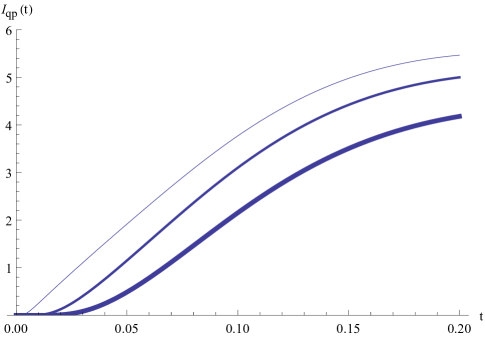
Figure 1: The dissipative part for the particle-hole contribution, $\frac{\zeta^{(R)}_{22,01}(\vec{Q},\Omega;qp)}{10^{-10}}\approx(\frac{Q_{1}}{q})(\frac{Q_{2}}{q})I_{pq}(t)\Big{[}\frac{Newton\cdot sec.}{m^{3}}\Big{]}$, with $I_{qp}(t)$ shown in Fig. 2.

Figure $1$ shows that the sound dissipative impedance is controlled by the absorption edge condition $\epsilon(b,k_{F})>t$ [here $t$ is the temperature and $\epsilon(b,k_{F})$ is the ground state energy determined by the magnetic field $b$]. Using the explicit formula $\epsilon(b,k_{F})=\epsilon_{0}(b,k_{F})-\frac{v}{2k_{F}}k^{2}_{F}\equiv\frac{vk_{F}}{2}\Big{(}\frac{1}{2\pi}\frac{q^{2}}{k^{2}_{F}}-1\Big{)}$, $\epsilon_{0}(b,k_{F})=\frac{vk_{F}}{2}\sqrt{\frac{b^{2}}{2}}$ given in Eq. $(11)$ we can determine from the impedance $\zeta^{(R)}_{22,01}(\vec{Q},\Omega;qp)$ the magnetic field $b$ and the vortex lattice constant $d$.

The absorption is given in units of $\frac{Newton\cdot sec.}{m^{3}}$. We plot $\frac{\zeta^{(R)}_{22,01}(\vec{Q},\Omega;qp)}{10^{-10}}$ for the case $\Delta=0.1$ meV and $\Omega=2\pi 10^{6}\frac{radians}{sec.}$ as a function of temperature $t$ ($t=0.1$ meV corresponds to $1$ Kelvin) and the vortex separation is $d=10^{-7}$ m. The function $I_{qp}(t)$ is shown for three different cases: The thin line gives the absorption for the ground state energy $\epsilon(b,k_{F})\equiv\frac{vk_{F}}{2}\Big{(}\frac{q^{2}}{8\pi k^{2}_{F}}-1\Big{)}=0.001$ mev, the thickest line represents the absorption for the ground state energy $\epsilon(b,k_{F})=0.1$ meV. The line in between describes the situation for $\epsilon(b,k_{F})=0.0075$ meV. We observe that the absorption edge temperature scales with the energy $\epsilon(b,k_{F})$ as a function of the magnetic field and Fermi energy.

b. Impedance for Majorana modes

The Majorana contribution given by the particle-hole [see Eq. $(21)$] depends on the tunneling amplitude $t_{0}$. We consider the ground state energies $\epsilon(b,k_{F})=0.005$ meV (thin line), $\epsilon(b,k_{F})=0.1$ meV (thick line) and $\epsilon(b,k_{F})=0.05$ meV (intermediate ground state energy).

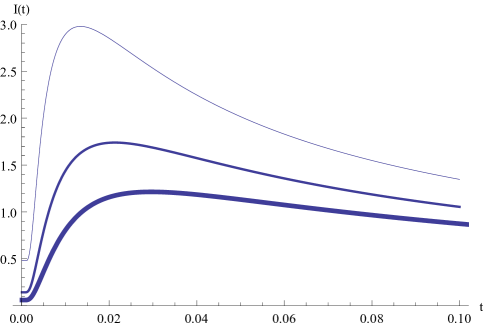
Figure 2: The dissipative impedance for Majorana particle-hole contribution $\frac{\zeta_{22,01}(\vec{Q},\Omega;0,\neq 0)}{10^{-10}}\approx(\frac{Q_{1}}{q})(\frac{Q_{2}}{q})10^{-2}I(t)\Big{[}\frac{Newton\cdot sec.}{m^{3}}\Big{]}$. The range of temperature is $0.005<t<0.1$ (temperature $t=1$ corresponds to $0.1$ meV and the structure for $t<0.005$ is an artifact of the numerics).

The Majorana contribution for the particle-particle part [see Eq. $(22)$] for the same values of $\epsilon(b,k_{F})$ and tunneling amplitude $t_{0}$ as in Fig. $(2)$ shows an absorption for low temperatures.

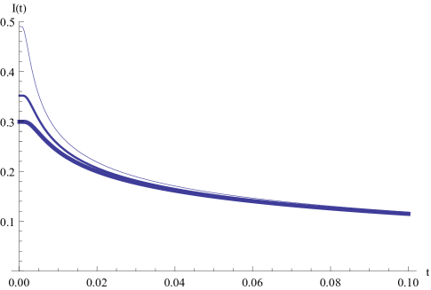
Figure 3: The dissipative impedance for Majorana particle contribution $\frac{\zeta_{22,22}(\vec{Q},\Omega;0,\neq 0)}{10^{-10}}\approx(\frac{Q_{1}}{q})(\frac{Q_{2}}{q})10^{-1}I(t)\Big{[}\frac{Newton\cdot sec.}{m^{3}}\Big{]}$ as a function of $\epsilon(b,k_{F})=0.005$ meV (thin line), $\epsilon(b,k_{F})=0.0075$ meV, $\epsilon(b,k_{F})=0.01$ meV (thick line). The range of temperature is $0.005<t<0.1$ (temperature $t=1$ corresponds to $0.1$ mev and the structure for $t<0.005$ is an artifact of the numerics).

Comparing Fig. $(1)$ with Figs. (2), (3) we observe that the Majorana fermion gives rise to absorption at low temperatures, in a region where the particle-hole absorption (Fig. $1$) is absent.

Since impurities are always present, it is important to know how to differentiate between the impurity absorption and the Majorana fermions. Impurities will give rise to absorption for frequencies $\Omega>\epsilon(b,k_{F})-\epsilon_{impurity}$ and for temperatures $T>\Omega$; on the other hand, the Majorana absorption persists at $T\rightarrow 0$ (see Fig. $3$).The total impedance is given by the sum of contributions in the three figures (1) - (3). We therefore conclude that the information about the Majorana modes, the magnetic field and tunneling amplitude $t_{0}$ can be obtained from the viscosity stress measurement.

VII. Comments on the sound wave analog of Andreev crossed reflection

Next we comment on the sound wave analog of the Andreev reflection. Two Majorana modes located at the two ends of a $p$-wave superconductor wire are detectable by piezoelectric transducers representing the sound equivalent of the two-leads experiments which measure the Andreev crossed reflection Flensberg ; DavidMajorana . We demonstrate that the same equations which were obtained for the Andreev crossed reflection Flensberg ; DavidMajorana induced by a voltage between the two tips are obtained for a sound wave which creates a time-dependent lattice deformation $D(t)=u(\frac{L}{2},t)+u(-\frac{L}{2},t)$. Here $u(\pm\frac{L}{2},t)$ is the sound deformation in the vicinity of each tip. The lattice deformation acts as a bias field. The voltage field $e^{\pm i\frac{e}{\hbar}Vt}$ in the two-tip experiment is replaced by a bias field $e^{\pm ik_{F}D(t)}$ for the sound wave case.

We follow the derivation given in refs. Flensberg ; DavidMajorana . For a $p$-wave (or equivalently a one-dimensional wire with spin-orbit interaction in the proximity of an $s$-wave superconductor and a magnetic field) with length $L$ we have two Majorana modes localized at $x=-\frac{L}{2}$ and $x=\frac{L}{2}$. The fermions for the two tips are represented by $C_{1}(x=-\frac{L}{2})=e^{ik_{F}(-\frac{L}{2})}R_{1}(x=-\frac{L}{2})+e^{-ik_{F}(-\frac{L}{2})}L_{1}(x=-\frac{L}{2})$ and $C_{2}(x=\frac{L}{2})=e^{ik_{F}(\frac{L}{2})}R_{2}(x=\frac{L}{2})+e^{-ik_{F}(\frac{L}{2})}L_{2}(x=\frac{L}{2})$. (Here $R_{1}$, $R_{2}$, $L_{1}$ and $L_{2}$ are the right and left chiral fermions and $k_{F}$ is the Fermi momentum of the electrons).

Following ref. DavidMajorana we integrate the Majorana fermions and obtain the coupling between the two tips: $H_{eff.}(t)=(-ig^{2})\int_{0}^{\infty}\,d\tau\chi^{+}(t)e^{-i\epsilon_{0}\tau}\chi(t-\tau)$ where $\epsilon_{0}$ is the overlap energy between the two Majoranas. Ignoring the oscillating terms $e^{ik_{F}(\pm\frac{L}{2})}$ allows us to simplify the form of $H_{eff.}$. In order to study the response to sound waves we replace $e^{\pm ik_{F}(\pm\frac{L}{2})}\rightarrow e^{\pm ik_{F}(\pm\frac{L}{2}+u(\pm\frac{L}{2}))}$, where $u(\pm\frac{L}{2})$ is the sound deformation induced by the transducer. The deformation field $D(t)=u(\frac{L}{2},t)+u(-\frac{L}{2},t)$ is a function of the transducer frequency $\Omega$. The velocity strain field is given by $\epsilon_{01}(t)=\partial_{t}D(t)$. The derivative of the effective Hamiltonian $H_{eff.}(t)$ with respect to the strain velocity $\epsilon_{01}(t)$ determines the momentum density $\pi(x,t)$,

$\pi(x,t)=\frac{\partial H_{eff.}(t)}{\partial(\partial_{t}D(t))}\approx(\frac{-ig^{2}k_{F}}{\epsilon_{0}})\theta[t]\Big{[}e^{ik_{F}D(t)}J(-\frac{L}{2},\frac{L}{2};t)+e^{-ik_{F}D(t)}J^{*}(-\frac{L}{2},\frac{L}{2};t)\Big{]}$

where

$$J\left(-\frac{L}{2},\frac{L}{2};t\right)\equiv L^{\dagger}_{2}\left(\frac{L}{2},t\right)R_{1}\left(-\frac{L}{2},t\right)-L^{\dagger}_{1}\left(-\frac{L}{2},t\right)R_{2}\left(\frac{L}{2},t\right)+R_{1}\left(-\frac{L}{2},t\right)R_{2}\left(\frac{L}{2},t\right)$$

$$+L^{\dagger}_{2}\left(\frac{L}{2},t\right)L^{\dagger}_{1}\left(-\frac{L}{2},t\right).$$

Here $J(-\frac{L}{2},\frac{L}{2};t)$ is the correlation between the tips; when a voltage is applied between the tips this correlation represents the current operator DavidMajorana .

From the momentum density we compute the dissipative viscosity and the time ordered correlation function, $R_{01,01}(q,\Omega)=(\frac{-i}{\hbar})\langle|T\Big{(}\pi(q,t)\pi(-q,0)\Big{)}|\rangle$. Following Eq. $(18)$ we obtain the viscosity $\zeta_{01,01}(q,\Omega)=-\frac{R_{01,01}(q,\Omega)}{i\Omega}$. The viscosity $\zeta_{01,01}(q,\Omega)$ is equivalent to the Andreev crossed reflection conductance obtained when voltage is applied between the tips Flensberg ; DavidMajorana . [To compare the two correlation functions we need to replace $\frac{e}{\hbar}Vt$ with $k_{F}D(t)$ and $g^{2}e$ with $\frac{g^{2}k_{F}}{\epsilon_{0}}$.]

VIII. Conclusions

In the first part of this paper we derived the spinor solution for an Abrikosov vortex lattice in a topological superconductor. We then obtained the zero and non-zero mode wave functions. These results have been used to compute the dissipative viscosity, which is obtained as a stress response to an applied velocity strain field. Experimentally one uses two transducers, one for measuring the stress response and the second transducer to generate the strain field. We find in addition to the particle-hole contribution, a viscosity term which reflects the presence of Majorana fermions. Probing the $p$-wave wire with a sound wave one thus finds an effect similar to the Andreev crossed reflection.

Apendix A. Vortex lattice

We consider the Hamiltonian given by Eq. $(2)$ in a magnetic field.

$$\hat{H}=\int\,d^{2}x\hat{\Psi}^{\dagger}(\vec{x})\Big{[}\tau_{3}\hat{h}_{3}+\tau_{2}\hat{h}_{2}+\tau_{1}\hat{h}_{1}\Big{]}\hat{\Psi}(\vec{x}),\hskip 1.8063pt\frac{1}{2}\vec{\partial}_{x}\theta(\vec{x})\equiv\frac{1}{2}\sum_{l}\vec{\partial}_{x}\varphi_{l}(\vec{x}),\varphi_{l}(\vec{x})\equiv\arg\Big{(}\vec{x}-\vec{R}_{l}\Big{)}$$

$$\hat{h}_{3}=\frac{v}{2k_{F}}\Big{(}\Big{(}-i\vec{\partial}_{x}-\frac{e}{\hbar}\vec{A}(\vec{x})+\frac{1}{2}\vec{\partial}_{x}\theta(\vec{x})\Big{)}^{2}-k^{2}_{F}\Big{)},\hskip 1.8063pt\hat{h}_{2}=i\frac{|\Delta(\vec{x})|}{2k_{0}}\partial_{1},\hskip 1.8063pt\hat{h}_{1}=-i\frac{|\Delta(\vec{x})|}{2k_{0}}\partial_{2}.$$

We consider first a single vortex in Eq. $(2)$ and find from the London equation that the effective magnetic field $b$ is replaced by a string-like solution Ezawa ; Tinkham , $b(\vec{x})=\frac{\Phi_{L}}{2\pi\lambda^{2}_{L}}K_{0}\Big{(}\frac{|\vec{x}-\vec{R}_{l}|}{\lambda_{L}}\Big{)}$ which vanishes for $|\vec{x}|\gg d$ ($d$ is the vortex lattice constant, $\lambda_{L}$ is the magnetic penetration depth and $K_{0}$ is the modified Bessel function). Since we are interested in constructing a periodic solution we replace the magnetic field for $|\vec{x}|<d\approx\lambda_{L}$ with a constant magnetic field. The constant magnetic field restricted to $|\vec{x}|<d$ is approximated by the spatial average around the core with a radius of $d$. In order to study the vortex properties we add to the superconducting Hamiltonian $\hat{H}$ [given in Eq. $(2)$] the magnetic energy $H_{M}$ and the condensation energy $H_{\Delta}$:

$$H_{eff.}=\hat{H}+H_{M}+H_{\Delta},$$

$$H_{M}=\int\,d^{2}x\left(\frac{1}{2\mu_{M}}\right)\Big{[}\partial_{1}A_{2}(\vec{x},t)-\partial_{2}A_{1}(\vec{x},t)\Big{]}^{2},$$

$$H_{\Delta}=\frac{1}{g}\int\,d^{2}x|\Delta|^{2},$$

where $A(x,t)$ denotes the vector potential and $\Delta$ is the gap parameter.

The variation of Hamiltonian $H_{eff.}$ in Eq.$(26)$ determines the London equation for a single vortex.

$$-\lambda^{2}_{L}b(\vec{x})+b(\vec{x})=\Phi_{L}\delta[\vec{x}-\vec{R}_{l}],$$

$$\lambda^{2}_{L}=\frac{k_{F}}{\mu_{M}e^{2}\rho},\hskip 7.22743pt\rho=\frac{v}{k_{F}}.$$

The solution of the London equation is: $b(\vec{x})=\frac{\Phi_{L}}{2\pi\lambda^{2}_{L}}K_{0}\Big{(}\frac{|\vec{x}-\vec{R}_{l}|}{\lambda_{L}}\Big{)}$ where $K_{0}$ is the modified Bessel function Tinkham . This string-like solution gives rise to the effective vector potential $A^{(i)}_{eff.}=2e\Phi_{L}\epsilon_{i,j}\frac{{x}_{i}}{2\pi r^{2}}\Big{(}\frac{|\vec{x}|}{\lambda_{L}}K_{1}(\frac{|\vec{x}|}{\lambda_{L}})-1\Big{)}$, $i=1,2$, $j=1,2$ ($\epsilon_{i,i}=\epsilon_{i,i}=0$, $\epsilon_{1,2}=1$, $\epsilon_{2,1}=-1$). As a result the field $|\hat{\Psi}_{\neq 0}(\vec{x})|^{2}$ vanishes at $\vec{x}=\vec{R}_{l}$ and is constant at large distances. For a periodic structure of vortices we find

$$-\lambda^{2}_{L}b(\vec{x})+b(\vec{x})=\Phi_{L}\sum_{l}\delta[\vec{x}-\vec{R}_{l}].$$ (28)

This equation shows that the effective magnetic field $b(\vec{x})$ for multi-vortices is periodic.

Appendix B. Majorana fermion localized at the origin

For a vortex which is localized at $\vec{x}=0$, the phase is $\varphi$. The vortex field $\theta_{v}(\vec{x})=\theta_{v}(r,\varphi)$ obeys $[\theta_{v}(r,\varphi=2\pi)-\theta_{v}(r,\varphi=0)]=2\pi N$ with $N=1$ Gurarie . The field $\hat{C}(\vec{x})=\hat{C}(r,\varphi)$ transforms as $\hat{C}(r,\varphi+2\pi)=-\hat{C}(r,\varphi)$ and $\hat{C}^{\dagger}(r,\varphi+2\pi)=-\hat{C}^{\dagger}(r,\varphi)$ in the presence of a multi-valued phase $\theta(\vec{x})$. Consequently, for a $2\pi$ vortex, the fields $\hat{C}(\vec{x})$, $\hat{C}^{\dagger}(\vec{x})$ are double-valued. This corresponds to a half-vortex, and a rotation of $2\pi$ implies a change of phase of $\pi$ in the fermion field. Using polar coordinates, we have $(\partial_{1}+i\partial_{2})\rightarrow e^{i\varphi}(\partial_{r}+\frac{i}{|\vec{x}|}\partial_{\varphi})$ and $(\partial_{1}-i\partial_{2})\rightarrow e^{-i\phi}(\partial_{x}-\frac{i}{|\vec{x}|}\partial_{\varphi})$. The kinetic energy in the presence of a vortex at the origin $\vec{x}=0$ becomes,

$$K.E.\approx\frac{v}{2k_{F}}\Big{(}-i\vec{\partial}_{x}\Big{)}^{2}-\mu_{eff.}(\vec{x}).$$ (29)

At the origin the effective chemical potential is positive far from the vortex and changes sign for $\vec{x}\rightarrow 0$. (A Majorana mode exists at the boundary of a trivial superconductor $\mu_{eff.}<0$ and a topological one with $\mu_{eff.}>0$),

$$\left[\begin{array}[]{rrr}-\mu_{eff.}(\vec{x}),&\frac{-|\Delta|}{2k_{0}}e^{i\varphi}(\partial_{x}+\frac{i}{r}\partial_{\varphi})\\ \frac{-|\Delta|}{2k_{0}}e^{-i\varphi}(\partial_{x}-\frac{i}{r}\partial_{\varphi}),&\mu_{eff.}(\vec{x})\\ \end{array}\right]\left(\begin{array}[]{cc}U_{0}(r,\varphi)\\ V_{0}(r,\varphi)\end{array}\right)=0.$$ (34)

The zero mode solution is given by: $W_{0}(r,\varphi)=\Big{[}U_{0}(r,\varphi),V_{0}(r,\varphi)\Big{]}^{T}\equiv\Big{[}\frac{1}{\sqrt{i}}e^{\frac{i}{2}\varphi},\frac{1}{\sqrt{-i}}e^{\frac{-i}{2}\varphi}\Big{]}^{T}\frac{F(r)}{\sqrt{r}}$. The function $\frac{F(r)}{\sqrt{r}}$ obeys the normalization condition $\int\,d^{2}r[\frac{F(r)}{\sqrt{r}}]^{2}<\infty$. For a vortex lattice we use the Majorana solution which is given at $x=0$ and is translated periodically.

Appendix C. Invariance of the Hamiltonian under the coordinate transformation: derivation of the stress-strain Hamiltonian

The viscosity tensor is obtained from the linear response of electrons in an external field Fetter . In order to accomplish this task we need to identify the elastic analog of the external electromagnetic field. This is accomplished using the invariance of the action under the coordinate transformation.

The unperturbed crystal is described by the coordinates $\vec{x}$ and the deformed crystal by the coordinates $\vec{\xi}$. The distortion of the crystal is given by $\vec{u}$ which is caused either by the phonons of the crystal or by an external force. We use the system $\xi^{a}$ to describe the orthonormal coordinates for the deformed crystal with the basis vector frame $\partial_{\xi^{a}}$, a=1,2,3. The unperturbed crystal is described by the Cartesian coordinates $x^{i}$ with the basis frame vectors $\partial_{x^{i}}$, i=1,2,3. The two coordinate systems in the two frames are related Katanaev :

$$\vec{x}\rightarrow\vec{\xi}(\vec{x})=\vec{x}+\vec{u}(\vec{\xi}),$$

$$\xi^{a}(\vec{x})=x^{a}+u^{a}(\vec{\xi}),~{}~{}a=1,2,3;\hskip 10.84006pt\xi^{i}(\vec{x})=x^{i}+u^{i}(\vec{\xi}),~{}~{}i=1,2,3,$$

where $i$ represents the Cartesian coordinates and $a$ represents the deformed crystal. When the deformation of the crystal $\vec{u}$ vanishes we have the relation $\vec{x}=\vec{\xi}$. This allows us to introduce the non-relativistic transformation of the derivatives:

$$\partial_{\xi^{a}}=\sum_{i=1,2,3}\frac{\partial x^{i}}{\partial_{\xi^{a}}}\partial_{i}=\sum_{i=1,2,3}\frac{\partial(\xi^{i}-u^{i})}{\partial_{\xi^{a}}}\partial_{i}=\sum_{i=1,2,3}(\delta_{i,a}-\partial_{a}u^{i})\partial_{i};a=1,2,3,$$

$$\frac{d}{dt}=\partial_{t}+\sum_{i=1,2,3}\partial_{t}u^{i}\partial_{i}.$$

The metric integration for the deformed space is given in terms of the crystal deformation vector field $\vec{u}$. That is, $dtd\xi^{a=1}d\xi^{b=2}d\xi^{c=3}=dt\mathbf{e}dx^{1}dx^{2}dx^{3},$ where $\mathbf{e}$ is the Jacobian of the coordinate transformation which for the two-dimensional case is given by: $\mathbf{e}=1-(\partial_{1}u^{1}+\partial_{2}u^{2})-\partial_{1}u^{1}\partial_{2}u^{2}$. We replace $\partial_{a}u^{j}\approx\partial_{i}u^{b}\delta_{a,i}\delta_{j,b}\approx\partial_{i}u^{j}$ (the exact relation is given by the matrix equation $\sum_{j}\partial_{a}u^{j}\partial_{j}u^{b}=\delta_{a,b}$). We introduce the notation $\epsilon_{i,j}=\frac{1}{2}\Big{(}\partial_{i}u^{j}+\partial_{j}u^{i}\Big{)}$, $\epsilon_{0,i}=\partial_{t}u^{i}$ and $\Omega_{i,j}=\frac{1}{2}\Big{(}\partial_{i}u^{j}-\partial_{j}u^{i}\Big{)}$. When the excitations are caused by the phonons, we use the phonon spectrum of the crystal (in the harmonic representation). Due to the compatibility conditions Kosevich we have $\Omega_{i,j}=0$ and for a crystal with disclinations we have $\Omega_{i,j}\neq 0$.

References

(1) Liang Fu and C.L. Kane, Phys. Rev. Lett. 102, 216403 (2009).
(2)
J.P. Xu, C. Liu, M.X. Wang, J. Ge, Z.L. Liu, X. Yang, Y.Chen, Y. Liu, Z.A. Xu, C.L. Gao, D. Qian, F.C. Zhang, and J.F. Jia,
Phys. Rev. Lett. 112, 217001 (2014).
(3) Eytan Grosfeld and Ady Stern, Phys. Rev. B 73, 201303R (2006).
(4)Ching-Kai Chiu, D.I. Pikulin, and M. Franz, Phys. Rev. B 91, 165402 (2015).
(5) Rudro R. Biswas, Phys. Rev. Lett. 111, 136401 (2013).
(6) Alexander V. Balatsky and Ivar Martin, Los Alamos Science, Number 27, (2002), arXiv: 0112407 (2001).
(7) M. Huefner, A.Pivonka, J. Kim, C. Ye, M .A. Blood-Forsythe, M.Z ech, and J.E. Hoffman, Applied Physics Letter 101, 173110 (2012).
(8) Remy Pawlak, Marcin Kissiel, Jelena Klinovaja, Tobias Meier, Shigeki Kawai, Thilo Glatzel, Daniel Loss, and Ernst Meyer, arXiv:1505.06780 (2015).
(9) J. Li, T. Neupert, B.A. Bernevig, and A. Yazdani. arXiv: 1404.4058 (2014).
(10) Stevan Nadj-Perge, Jian Li, Hua Chen, Sangjun Jeon, Jungpil Seo, Alan MacDonald, B. A. Bernevig, Ali Yazdani, Science 346, 1259327 (2014).
(11) K. Flensberg, Phys. Rev. B, 82, 180516 (2010).
(12) D. Schmeltzer “The Andreev crossed reflection – a Majorana path integral approach”, arXiv:1508.00024; Journal of Modern Physics 6, 1371 (2015).
(13) J.R. Schrieffer, “Theory of Superconductivity”, (Benjamin, New York ,1964).
(14) Thomas Aref, Per Delsing, Maria K. Kockum, Martin V.Gustafson, Goran Johansson, Peter Leek, Einar Magnusson, and Riccardo Manenti, arXiv:1506.01631 (2015).
(15) E.B. Magnusson, B.H. Williams, R. Mannenti, M.-S. Nerisisyan, M.J. Peterrer, A. Ardavan, and P.J. Leek, Applied Physics Letters 106, 063509 (2015).
(24) M.S.Marenko, C.Bourbonnais, and A.M.S.Tremblay,
arXiv:0412553 (2004).
(25) S. Murakawa, Y. Tamura, Y. Wada, M. Wasai, M. Saitoh, Y. Aoki, R. Nomura, Y. Okuda, Y. Nagato, M. Yamamoto,
S. Higashitani, and K. Nagai, Phys. Rev. Lett. 103, 155301 (2009).
(26) L.D. Landau and E.M. Lifshitz, “Theory of Elasticity ”, (Pergamon, Oxford, 1959).