Predicting the evolution of complex networks via local information

Abstract

Almost all real-world networks are subject to constant evolution, and plenty of evolving networks have been investigated to uncover the underlying mechanisms for a deeper understanding of the organization and development of them. Compared with the rapid expansion of the empirical studies about evolution mechanisms exploration, the future links prediction methods corresponding to the evolution mechanisms are deficient. Real-world information always contain hints of what would happen next, which is also the case in the observed evolving networks. In this paper, we firstly propose a structured-dependent index to strengthen the robustness of link prediction methods. Then we treat the observed links and their timestamps in evolving networks as known information. We envision evolving networks as dynamic systems and model the evolutionary dynamics of nodes similarity. Based on the iterative updating of nodes’ network position, the potential trend of evolving networks is uncovered, which improves the accuracy of future links prediction. Experiments on various real-world networks show that the proposed index performs better than baseline methods and the spatial-temporal position drift model performs well in real-world evolving networks.

1 Introduction

Complex networks involve the characterization of complex systems of interacting entities, where nodes denote the entities and links represent the relationships or interactions between them. Complex networks provide an ideal tool for understanding the structure and function of many complex systems in nature, technology and society [1]. With great brilliance, various kinds of methods have been proposed to address the network analysis problem, including community detection [2, 3], cascades prediction [4, 5], network controllability [6], etc. In particular, the evolution trend, which describe the grow and change of network topology through the addition or deletion of nodes and links, is a critical aspect of network analysis. Up to now, the evolution mechanisms that have been preliminarily verified include preference attachment [7], small world [8], homophily [9], clustering [10], etc. Since uncovering how real-world networks are evolved can considerably deepen the understanding about many complex systems and guide the behavior of individuals, the question which we will address here is how to predict the evolution trend of complex networks without losing generality. According to Ref. [11], an effective link prediction algorithm provides strong evidence of the corresponding mechanism(s) of network organization. Here, we will in fact answer the question by developing a structure-dependent link prediction index for ranking the candidates of future links and an explicit spatial-temporal network position drift model for uncovering the potential trend of network evolution.

In recent years, link prediction problem has attracted a considerable amount of attention in complex network studies [12-15]. Especially, D. Liben-Nowell et al. [15] argue that the link prediction problem asks to what extent can the evolution of a complex network be modeled using features intrinsic to the network itself ? They summarize many similarity indices based on network structure and find that there is indeed useful information contained in the network topology alone by comparing them with random predictors. Commonly, the topology-based methods can be divided into three classes. The first class is similarity-based methods, which assume that links between more similar nodes are of higher existing likelihood, and the similarity of the two endpoints can be transferred through the links. The similarity-based methods can be subdivided into neighbor-based methods and distance-based methods. Neighbor-based methods are based on the idea that two nodes are more likely to generate a link in the near future if they have more common neighbors, such as Sorensen [16], LHN [17], CN[18], etc. Distance-based methods suppose that link probability is determined by distance or number of the shortest path between nodes, such as LP [19], Katz [20], LHN-II [17], etc. The second class of link prediction methods is maximum likelihood estimation methods. Two popular methods of this type are the hierarchical structure model (HSM) [21] and the stochastic block model (SBM) [22]. The third class of link prediction methods is machine learning based methods. The main methods of this type are the supervised learning method [23] and negative matrix factorization (NMF) mehtod [24]. Owning to its simplicity, the study on similarity-based algorithms is the mainstream issue.

However, in most of the existing works, a typical method is to consider an algorithm’s accuracy in reproducing known network links that have been removed from a test dataset. An accurate prediction, however, is not necessarily a useful one. Specially speaking, the distinction between future links prediction and missing links prediction is actually never that clear, while Ref. [25] offers evidence that missing links are more likely to be the links connecting low-degree nodes. As almost all real-world networks are evolving all the time [26], one has to investigate the evolution trend of networks, i.e., what are the future links of evolving networks. This is not a trivial problem. It has already been pointed out that many new members are the neighbors or second level neighbors of the current group members and they are more likely to join the group with the clustering of the group increases from a group-level perspective in evolving real-world networks [27, 28]. That is to say, node groups with higher clustering level are more likely attract nodes than the uncompacted ones. Furthermore, the result of Ref. [29] shows that the auto-correlation function of the successive states of communities is continuous, which indicates that the current states of networks are associated with the states at the last time point. Next the Ref. [30] recognizes a pattern that links are highly biased towards young nodes. Thus the timestamps of network interactions signified by network links has the potential to hint the trend of network evolution. However, how all these factors influence the future links prediction still remain unclear. Therefore, it is necessary to explore the problem of evolving networks prediction in combination with these factors.

In this paper, in order to adapt to networks with different structure properties, we propose a structure-dependent index combining the virtues of neighbor-based methods and distance-based methods. Moreover, unlike the existing link prediction methods which assume the similarities of nodes are constant, we envision evolving networks as dynamic systems and investigate the evolutionary dynamics of similarities. The structure features of nodes’ neighborhood and the timestamps of network interactions are called spatial factor and temporal factor respectively. Combining the spatial and temporal factors, we propose a dynamic network position drift model, in which node’s network position undergoes migration and variation under the influence of its neighbors’ attractiveness. The variation of node’s network position reflects the potential trend underlying the current network structure, and the iterative updating of node’s network position would lead to an evolved network representing the similarity relationships of network nodes in the near future. Finally, according to the empirical results on five real-world networks, we find that the structure-dependent index is effective and robust for link prediction and the spatial-temporal position drift model has satisfactory performance.

The rest of the paper is organized as follows. Section 2 introduces some indices as baselines. Section 3 presents the structure-dependent index and the spatial-temporal position drift model. Section 4 gives the empirical analysis. Discussion and conclusion are drawn in Section 5.

2 Preliminaries

2.1 Problem and evaluation

Consider an undirected simple network $G=(V,E)$, where $V=\{v_{i}\}$ is the set of nodes and $E$ is the set of links. Multiple links and self-connections are not allowed. Each link $e=(u,v,t)\in E$ represents an interaction between $u$ and $v$ that took place at time $t$. Let $G[t,t^{\prime}]$ denote the subgraph of $G$ consisting of all links with timestamps between $t$ and $t^{\prime}$. We choose three timestamps ${\rm{t}}_{0}{\rm{<t}}_{\rm{1}}{\rm{<t}}_{\rm{2}}$ and get subgraph ${\rm{G[t}}_{\rm{0}}{\rm{,t}}_{\rm{1}}{\rm{]}}$ and ${\rm{G[t}}_{1}{\rm{,t}}_{2}{\rm{]}}$. We refer to ${\rm{[t}}_{0}{\rm{,t}}_{1}{\rm{]}}$ as the training interval and ${\rm{[t}}_{1}{\rm{,t}}_{2}{\rm{]}}$ as the probe interval. Commonly, networks grow through the addition of nodes and links, and it is not sensible to predict the links of $G[t_{1},t_{2}]$ whose endpoints are not present in $G[t_{0},t_{1}]$. Thus we eliminate the new added nodes within $[t_{1},t_{2}]$. We define $ET$ and $EP$ to denote the set of links in $G[t_{0},t_{1}]$ and $G[t_{1},t_{2}]$ respectively. Clearly, we have $ET\cap EP=\emptyset$. We use $U$ to denote the universal set containing all $|V^{\prime}|(|V^{\prime}|-1)/2$ possible links, where $V^{\prime}$ denotes the set of nodes in $G[t_{0},t_{1}]$.

In link prediction, $ET$ is treated as known information while $EP$ is only used to test the accuracy. For each pair of nodes $u$, $v$ $\in V^{\prime}$ without a link in $G[t_{0},t_{1}]$, each link predictor that we consider assigns a similarity score based on the existing links in $ET$. Then all unlinked pairs are ranked in descending order according to their scores. In this study, we use two evaluation metrics, AUC (Area Under the Receiver operating characteristic curve) and precision. In the present case, AUC can be simplified as the probability that a randomly chosen link in $EP$ has higher similarity score than a randomly chosen nonexistent link in ${U\backslash(ET\cup EP)}$. In the evaluation implementation, among $n$ times of independent comparisons, if there are $n^{\prime}$ times that the future link has a higher score and $n^{\prime\prime}$ times the future link and nonexistent link have the same score, then AUC can be calculated by ${\rm{AUC}}=\frac{{n^{\prime}+0.5n^{\prime\prime}}}{n}$. If all the scores are generated from an independent and identical distribution, AUC will be approximately 0.5. Therefore, the extent to which AUC exceeds 0.5 indicates how much better the algorithm performs than pure chance. We compare the first $L$, $L=|EP|$, links with $EP$ to compute the precision of a predictor. Given the ranking of the non-observed links ${U\backslash ET}$ in which there are some future links, if $Lr$ links among top-$L$ links are accurately predicted ($Lr$ is the number of the top-$L$ links in the probe set $EP$), then ${\rm{Precision}}=Lr/L$. In this paper, our fundamental hypothesis is that the addition of a set of links does not significantly change network’s structure features, and we make sure training set representing a connected network in empirical analysis.

2.2 Similarity indices

Among many similarity indices, Liben-Nowell and Kleinberg [15] and Zhou et al [19] showed that Common Neighbors (CN), Adamic-Adar (AA) and Resource Allocation (RA) indices perform best by systematically comparing local similarity indices in unweighted networks. Therefore, in this paper, we concentrate on the weighted definition of these three indices (denoted by WCN, WAA, WRA respectively) and more details can be found in Ref. [12].

$$s_{xy}^{WCN}=\sum\limits_{z\in\Gamma(x)\cap\Gamma(y)}{w(x,z)+w(z,y)}$$ (1)

$$s_{xy}^{WAA}=\sum\limits_{z\in\Gamma(x)\cap\Gamma(y)}{\frac{{w(x,z)+w(z,y)}}{{\log(1+s(z))}}}$$ (2)

$$s_{xy}^{WRA}=\sum\limits_{z\in\Gamma(x)\cap\Gamma(y)}{\frac{{w(x,z)+w(z,y)}}{{s(z)}}}$$ (3)

Here, ${w(x,y)=w(y,x)}$ denotes the weight of the link between node $x$ and $y$, and $s(z)=\sum\nolimits_{z^{\prime}\in\Gamma(z)}{w(z,z^{\prime})}$ denotes the strength of node $z$, namely the sum of weights of its associated links. Moreover, we also take Local Path (LP) [19] index into account:

$$s_{xy}^{LP}=A^{2}+\varepsilon\cdot A^{3}$$ (4)

where $A$ is the adjacent matrix of network, and $e$ is a free parameter. LP index makes use of the information on local paths with lengths 2 and 3. In the real implementation, we directly count the number of different paths with length 2 and 3 and the parameter is fixed at $\varepsilon={\rm{10}}^{-3}$ following the original article [19]. In weighted networks, we sum up the weights of different paths with length 2 and 3.

3 Method

Prediction of evolving networks attempts to predict future network structure by mining data on past node interactions. From the perspective of dynamics, the dynamical evolution of complex networks can be simply given by the dynamical states in the phase space of the network, and the network dynamics can be decomposed into products of single node dynamics. What most have in common of the existing indices is that they fix the node similarities in prediction process. Here, we present a novel angle of view for future links prediction. The basic philosophy is to envision evolving networks as dynamic systems and dynamically investigate nodes’ similarities to uncover network’s evolutionary trend. The viewpoint provides a vivid and intuitive image to model the real-world network evolution. Before introducing the dynamics evolutionary model, we firstly present a rather robust and general similarity index by exploiting different range of structure information under the guidance of network macroscopical properties as follows.

3.1 Structure-dependent similarity index

Although for many networks with high clustering coefficient, neighbor-based methods, such as CN, AA, RA, can obtain satisfactory prediction accuracy. However, in some sparse networks with low clustering coefficient, it is difficult for neighbor-based methods to achieve high prediction accuracy. This may be because such neighbor-based indices cannot calculate similarity between nodes without common neighbors. Moreover, the neighbor-based methods are less distinguishable from each other, and the probability that two node pairs are assigned the same score usually is high [13]. To resolve the weaknesses of lower prediction accuracy, some distance-based methods are proposed, such as LP [19], Katz [20] and LHN-II [17]. However, the distance-based similarity indices are always sensitive to the proportion of observed edges. It means that their prediction accuracies will reduce obviously if the proportion of observed links decreases in training set. This is because the removal of links will increase the average shortest distance between node pairs. Thus, if the path range of distance-based indices smaller than the shortest distance between node pairs, the indices entirely cannot capture the similarities between the node pairs.

Based on the above analysis, it is necessary that proposing a rather robust and general similarity index for future links prediction. To strengthen the robustness of indices and calculate the similarity of node pairs in networks with different structure properties, similarity indices should count all possible paths between the nodes. However, the computation complexity of similarity index increases exponentially with the growth of the range of paths. As a result, we propose a structure-dependent (SD) similarity index exploiting different range of local structure information based on network macroscopical properties. The formal definition is given as follows:

$$s_{xy}^{SD}=\frac{{A^{s}}}{{\overline{k(z)}}}+\varepsilon\cdot\frac{{A^{s+1}}}{{\overline{k(z)}}}$$ (5)

where $A$ is the adjacent matrix, $k(z)$ denotes the degree of node $z$, $\overline{k(z)}$ is the average degree of the intermediate nodes between $x$ and $y$, $s$ is the shortest distant between node $x$ and $y$ and $s\leq\max(<d>,2)$, $<d>$ is the average shortest distant between node pairs. The weighted structure-dependent (WSD) index is defined as follows:

$$s_{xy}^{WSD}=\frac{{W^{s}}}{{\overline{s(z)}}}+\varepsilon\cdot\frac{{W^{s+1}}}{{\overline{s(z)}}}$$ (6)

where $W$ is the weight matrix, $s(z)$ denotes the strength of node $z$, $\overline{s(z)}$ is the average node strength of the intermediate nodes between $x$ and $y$, $\varepsilon$ is a free parameter. In the real implementation, we directly sum up the weights of the different paths with length $s$ and $s+1$ and the parameter is fixed at $\varepsilon={\rm{10}}^{-3}$ following the definition of LP [19]. According to the definition, we can find that WSD captures the shortest paths and the next shortest paths for similarity calculation. Furthermore, WSD reduces to WLP when the shortest distant is two and the average node strength $\overline{s(z)}$ equals to one, and WSD index reduces to WRA when range of the shortest distant is two and the parameter $\varepsilon$ is zero.

3.2 Spatial-temporal network position drift model

Spatial-temporal network position drift model is about the problem of how network nodes displace their network position to represent the potential trend of network evolution considering the spatial and temporal factors. Nodes’ network position is the similarity relationships between the nodes and their neighbors. As nodes interact only with their neighbors, the migration and variation of nodes’ network position can only be achieved via local interactions. Moreover, assuming that the link weight of two connected nodes indicates their interaction strength and the larger link weight represents the closer relationship between them, we set the link weights as the initial similarities of the connected nodes.

Fig. 1: The illustration of the spatial-temporal interaction model. (a) The graph representation of spatial interaction within local topology. (b) The graph representation of temporal interaction. (c) Force difference based spatial-temporal network position drift. (Arrows indicate the force difference between spatial-temporal influence and bond strength, and the node distance in the two subgraphs is proportional to the similarity and influence strength between them respectively.)

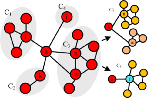
Spatial factor. To model the spatial influence, this paper assumes that network nodes are placed in force fields. To a network node, the attractiveness of all the node’s neighbors influence the central node’s network position. According to Ref. [27, 28], network nodes tend to approach the close connected groups and be far away from the uncompacted ones. Based on in-depth analysis of local structure, we find that each node has different network connection ability for structure organization. Commonly, the higher clustering level of groups that a node belongs to, the more and the stronger interactions within the node’ neighborhood, and the higher connection ability of the node. So network nodes tend to approach the nodes with high connection ability from the perspective of microstructure. To measure the influence of network nodes, this paper calculates the connection abilities of network nodes as their attractiveness. As nodes interact only with their neighbors, every network node takes all the attractiveness of its neighbors into account and then decide the direction and scale of position drift. Let’s take central node $a$’s neighbor node $i$ and $j$ in Fig. 1(a) for example. There are multiple edges in the one-hop neighborhood of node $i$, and $j$ is an isolated node. Thus node $i$ has higher connection ability and attractiveness than that of node $j$, and node $a$ will tend to approach node $i$ rather than node $j$. It is also possible that the interactions between node $a$ and the neighbors of node $i$ will be encouraged and strengthened. Formally, considering the link number and the link weight in one-hop neighborhood of network nodes, the attractiveness of them is defined as follows:

$$AI(j)=cn(j)\cdot st(j)=\sum\limits_{l\in Edge(ego(j))}{w_{l}}$$ (7)

where $ego(j)$ is the set of nodes in the one-hop neighborhood of node $j$, $Edge(ego(j))$ is the set of links between the nodes in $ego(j)$, $w_{l}$ is the weight of link $l$, $cn(j)=|E(ego(j))|$ is the connectivity ability of node $j$, and $st(j)=\sum\limits_{l\in E(ego(j))}\frac{{w_{l}}}{|E(ego(j))|}$ is the connectivity strength of node $j$.

Except for the interactions between the central node and its neighbors, there also may have interactions between the neighbors. In such situation, the neighbors and the central node form a triadic closure, and the connected neighbors would influence the central node consistently. The integrated attractiveness of the connected neighbors to the central node is different from the independent influence of anyone of the neighbors. Let’s take the neighbor node $m$ and $n$ in Fig. 1(a) for example, here, node $m$ and $n$ have a consistent and common attractiveness to the central node $a$ in Fig. 1(a), which is different from the independent influence of node $m$ or $n$ shown in the top right corner of Fig. 1(a).

To measure the attractiveness of the node $m$ and $n$ to the central node $a$, node $m$ and $n$ is considered as a whole to analyze. We fuse the neighborhood of node $m$ and $n$ as a new node $f$, as shown in the bottom right corner of Fig. 1(a), and measure the attractiveness of the new node to denote the attractiveness of node $m$ and $n$ proportionally. Formally, the attractiveness of a node in the connected neighbor set can be calculated by:

$$AI(i)=|NC|\cdot AI(v)\cdot\frac{{AI^{\prime}(i)}}{{\sum\nolimits_{j\in NC}{AI^{\prime}(j)}}}$$ (8)

where $NC$ is the connected neighbor set, ${AI(v)}$ is the attractiveness of the virtual node fused from $NC$, and ${AI^{\prime}(i)}$ is the attractiveness of node $i$ in independent situation. Let’s take node $m$ and $n$ in Fig. 1(a) for example, $AI(m)=2AI(f)\cdot\frac{{AI^{\prime}(m)}}{{AI^{\prime}(m)+AI^{\prime}(n)}}$, $AI(n)=2AI(f)\cdot\frac{{AI^{\prime}(n)}}{{AI^{\prime}(m)+AI^{\prime}(n)}}$, where ${AI(f)}$ is the attractiveness of the new node, $AI(f)=\sum\limits_{l\in Edge(ego(m))\cup Edge(ego(n))}{w_{l}}$, ${AI^{\prime}(m)}$ and ${AI^{\prime}(n)}$ are the attractiveness of node $m$ and $n$ in independent situation as shown in the top right corner of Fig. 1(a). Clearly, we have $AI(m)+AI(n)=2AI(f)$. What is worth noticing is that the connected neighbors have common intention and consistent behavior in attracting the central node.

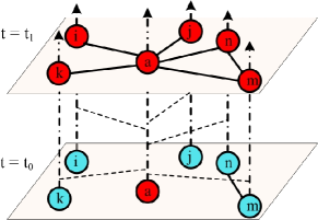
Temporal factor. According to the results of Ref. [29, 30], this paper assumes that the evolution process of networks is continuous and future state of evolving network is more relevant with the current state than the past states in evolution trend prediction. That is to say, more recent interactions are more powerful for potential trend indication of evolving networks than the older ones. To the central node $a$ in Fig. 1(a), the temporal dynamics can be illustrated by Fig. 1(b), and the interaction set of node $a$ can be represented as {$l_{aj}$, $l_{ai}$, $l_{an}$, $l_{ak}$, $l_{am}$} in timestamp sequence. With the growth of survival time, the indicative power of the interactions is reduced gradually. As a result, the temporal importance of link $l_{ai}$ for future links prediction is defined as

$$PI(l_{ai})=\frac{{e^{(t(l_{ai})-\overline{t(\{l_{a}\})})/2\Delta t}}}{{1+e^{(t(l_{ai})-\overline{t(\{l_{a}\})})/2\Delta t}}}$$ (9)

where $\overline{t(\{l_{a}\})}$ is the average of timestamps $\{l_{a}\}$, $\overline{t(\{l_{a}\})}=\frac{{\sum\nolimits_{j\in N(a)}{t(l_{aj})}}}{{|N(a)|}}$, $\Delta t$ is the unit time interval, $\Delta t=\frac{{\mathop{Max}\limits_{i\in N(a)}t(l_{ai})-\mathop{Min}\limits_{j\in N(a)}t(l_{aj})}}{{|N(a)|}}$, $t(l_{ai})$ is the timestamp of interaction between node $a$ and $i$, and $N(a)$ is the neighbor set of node $a$.

Based on the above analysis, the spatial-temporal influence of each neighbor $j$ on central node $i$ is comprehensively defined as:

$$A(j)=\frac{{AI(j)}}{{\mathop{\max}\limits_{k\in N(i)}AI(k)}}\cdot\frac{{PI(l_{ij})}}{{\mathop{\max}\limits_{k\in N(i)}PI(l_{ik})}}$$ (10)

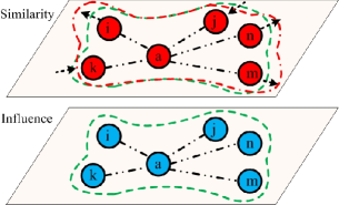
Spatial-temporal Position Drift. After modeling the spatial-temporal influence of every neighbors, how should nodes drift their network position according to the spatial-temporal influence? As analyzed in the local interaction process, all neighbors have spatial-temporal influence on the central node. In fact, every neighbor attracts the central node to move towards itself through mutual interactions. In order to establish the optimum trade-off among the spatial-temporal influence of every neighbors, the neighborhood of the central node can be regarded as a force field of node influence. Meanwhile, the similarities between the central node and its neighbors denote the current bond strength of them. Motivated by comparison of the spatial-temporal influence and the bond strength in the neighborhood of the central node, we argue that the direction and scale of position drift are all arise from the force difference between them. If the influence of an neighbor node on the central node is greater than the bond strength between them, the similarity between them increases. Conversely, the similarity decreases. As illustrated by Fig. 1(c), the arrows indicate the force difference between the spatial-temporal influence and the bond strength, where the distance between node pairs is proportional to the similarity and influence strength between them. Based on the above philosophy, we define $\Delta{{s(a,j)}}$ to characterize the dynamic of similarity ${{s(a,j)}}$ between node $a$ and $j$, ${{j}}\in{{N(a)}}$:

$$\Delta s(a,j)=-{\sum\limits_{k\in N(a)}{s(a,k)}}(\frac{{s(a,j)}}{{\sum\limits_{k\in N(a)}{s(a,k)}}}-\frac{{A(j)}}{{\sum\limits_{k\in N(a)}{A(k)}}})$$ (11)

4 Empirical Analysis

In this section, to demonstrate the benefits of the proposed method, we apply it on real-world networks for empirical analysis.

4.1 Data description

The dataset studied in this paper, including two static networks and three evolving networks, are detailed as follows. (1) Celegans [8]: The neural network of C. Elegans. (2) USAir [31]: The US Air transportation network. (3)MIT [32]: The network contains human contact data among 100 students of the Massachusetts Institute of Technology (MIT), collected by the Reality Mining experiment performed in 2004 as part of the Reality Commons project. (4) Hypertext 2009 network [33]: The network represents the face-to-face contacts of the attendees of the ACM Hypertext 2009 conference. Node represents a conference visitor, and an edge represents a face-to-face contact that was active for at least 20 seconds. Each edge is annotated with the time at which the contact took place. (5) Infectious network [33]: The network describes the face-to-face behavior of people during the exhibition INFECTIOUS: STAY AWAY in 2009 at the Science Gallery in Dublin. Nodes represent exhibition visitors, and edges represent face-to-face contacts that were active for at least 20 seconds. The basic structure properties of the networks are summarized in Table 1. The original networks are turned into undirected and simple networks.

Table 1: The basic structure properties of the giant components of the five example networks. $N$ and $M$ are the total numbers of nodes and links, respectively. $\langle k\rangle$ is the average degree of the networks. $\langle d\rangle$ is the average shortest distant between node pairs. $C$, $C_{w}$ and $r$ are clustering coefficient, weighted clustering coefficient and assortative coefficient, respectively. $H$ is the degree heterogeneity, defined as $H=\frac{{\langle k^{2}\rangle}}{{\langle k\rangle^{2}}}$, where $\langle k\rangle$ denotes the average degree.

4.2 Effectiveness and robustness of similarity index WSD

To verify the effectiveness of the proposed index WSD, we compare the prediction accuracy of different similarity index under the AUC metric and the Precision metric. The results are shown in Table 2 and Table 3 respectively. The metrics are introduced in the Preliminaries section. The highest AUC/Precision value for each network is shown in boldface. Under the AUC metric, WSD performs best in 3 out of 5 networks and performs next best in the other 2 networks, while WSD performs best in all of them under the Precision metric. In addition, we compare the prediction accuracy of different similarity index under varied ratio of deleted links in training set, and Fig. 2 shows the results of the methods. It can be seen that the proposed index is either the best or very close to the best in the five real-world networks. So we can conclude that the proposed WSD index is competitive to the state-of-the-art methods.

Table 2: Comparison of the prediction accuracy under the AUC metric in real-world networks.

Table 3: Comparison of the prediction accuracy under the Precision metric in real-world networks.

Fig. 2: Effectiveness of similarity index WSD under varied ratio of deleted links in five real-world networks. (The horizontal axis denotes the ratio of deleted links in training set for future links prediction. Each value of the Precision is a result averaged over 15 implementations with independent random divisions of the training set (90%) and the probe set (10%) in static networks and timestamps based orderly divisions of the training set (90%) and the probe set (10%) in evolving networks.)

(a) Robustness of similarity index WSD with different ratio of deleted links

(b) Average shortest distant between node pairs with different ratio of deleted links

Fig. 3: The illustration of the robustness of similarity index WSD. (The horizontal axis denotes the ratio of deleted links in training set for future links prediction. Each value of the Precision is a result averaged over 15 implementations with independent random divisions of the training set (90%) and the probe set (10%) in static networks and timestamps based orderly divisions of the training set (90%) and the probe set (10%) in evolving networks.)

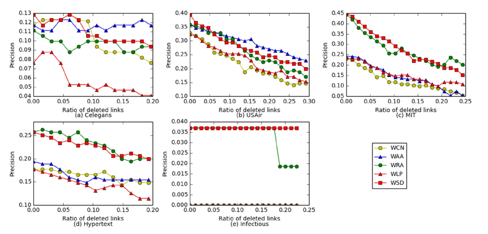
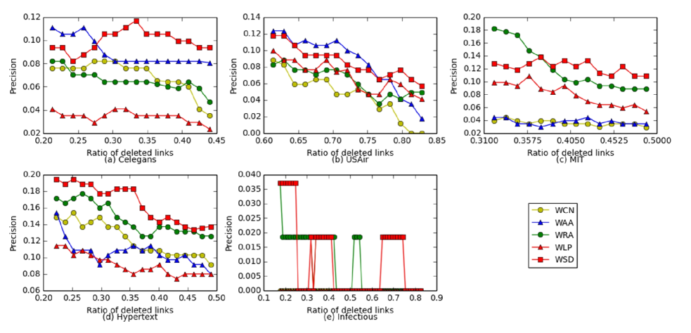
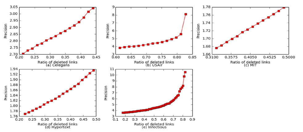
As discussed in section 3.1, neighbor-based indices cannot calculate the similarity of nodes without common neighbors and distance-based indices cannot capture the similarity of nodes if the path range of the distance-based indices is smaller than the shortest distance between the nodes. For example, looking at Table 3 and Fig. 2(e), for the prediction precision of the links in network Infectious, WCN, WAA and WLP are completely useless and the performance of WRA is also unsatisfactory. The main reason is that the average shortest distant 3.482 of network Infectious is greater than the path range 2.0 of similarity indices WCN, WAA, WRA and the the path range 3.0 of similarity index WLP. Hence, the indices cannot capture the similarities of the nodes in network Infectious. In contrast, WSD captures the shortest paths and the next shortest paths for similarity calculation under the guidance of networks’ structure properties.

Fig. 3 inspects the robustness of the proposed index WSD by comparing the prediction accuracy of different indices under varied ratio of deleted links. Intuitively, the more the amount of the deleted links, the less the amount of known information and the larger the average shortest distant. Fig. 3(a) describes a general trend of descending in prediction precision and Fig. 3(b) describes a general trend of ascending in average shortest distant with the growth of the ratio of deleted links. Synthesizes the results of Fig. 3(a) and Fig. 3(b), what calls for special attention is that WSD has satisfactory performance in the real-world networks and its advantage comparing the other similarity indices increase gradually with the increase of the average shortest distant. So WSD is robust in real-world networks with different structure properties.

4.3 The effectiveness of position drift on future links prediction

Fig. 4: The sensitivity of iteration number of position drift on link prediction. (Each value of the Precision and AUC is a result averaged over the similarity indices and 15 independent implementations with timestamps based orderly divisions of the training set (90%) and the probe set (10%) in evolving networks.)

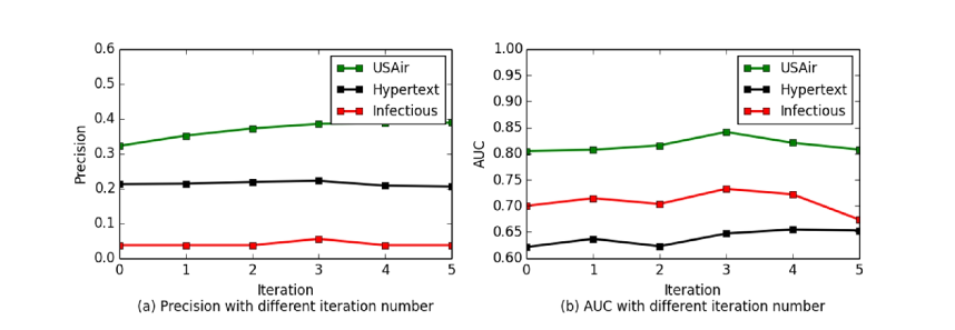
For uncovering the potential trend of network evolving, network nodes update their network position iteratively according to spatial-temporal position drift model in Eq. (11). Then link prediction methods calculate node similarity based on the drifted network topology. As different iteration number of position drift would lead to different network topology and different prediction accuracy, here, we study the influence of the iteration number on the evolving network prediction. The result is plotted in Fig. 4 with iteration number ranging from 0 to 5 on three evolving real-world networks. From this plot, we can see that the overall optimal performance is got when the iteration number equals to 3.

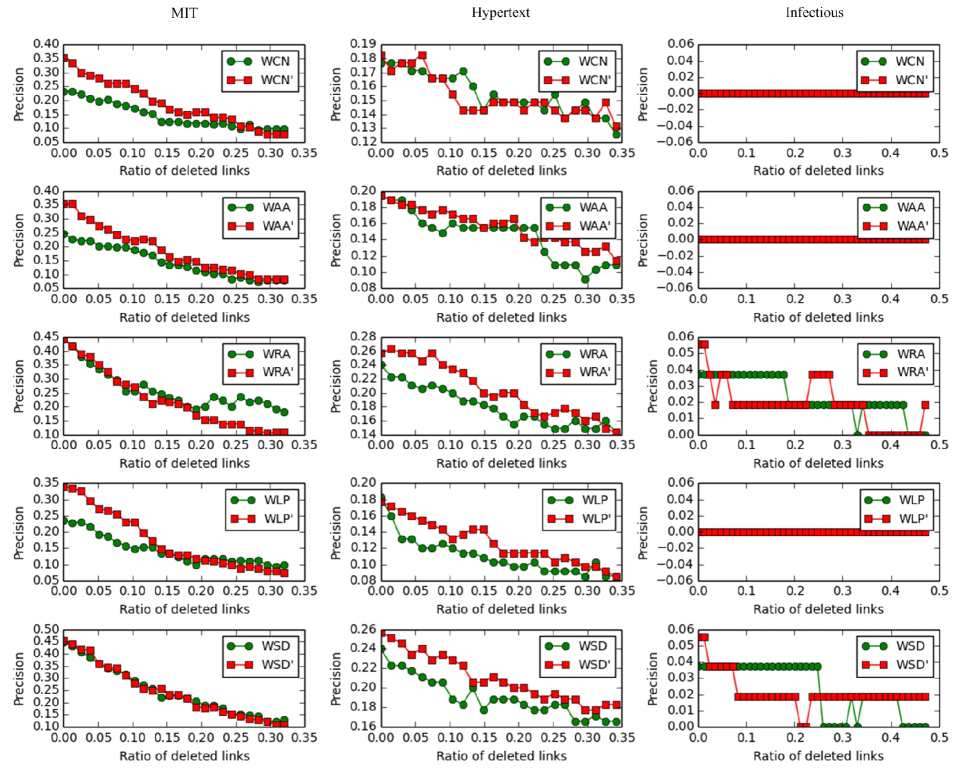
To each evolving network, every network node apply the position drift model to displace their network position firstly, then future links are predicted using the similarity indices on the drifted network. We compare the prediction accuracy with the result obtained based on the original network topology under the AUC metric and the Precision metric. From Table 4 and Fig. 5, it can be seen that the prediction results based on the drifted networks are either close to or better than the result obtained based on the original network topology, and the spatial-temporal position drift is effective for the evolving networks.

Table 4: The effectiveness of position drift on future links prediction under the AUC metric.

4.4 Running time

Table 5 presents the computation time of the link prediction methods and the position drift model with varied iteration number. As WAA, WRA are variants of WCN, they have nearly the smallest computation values in the real-world networks. WLP captures the information of paths with two and three hops and needs more computation time than that of WCN, WAA, WRA. Compared with WLP, the WSD index achieves competitive performance in all the networks. In addition, to position drift model, each node displace its network position based on the attractiveness of its neighbors, so its computational complexity is sensitive to the average degree of network. According to Table 5, we can find that the computation times on the three evolving networks decrease with the decline of the average degree of the networks. Since the real-world networks are mostly sparse, the position drift model is practical in realistic application. In summary, the proposed prediction index and the position drift model are all practical from the perspective of computation time.

Fig. 5: The effectiveness of position drift on future links prediction under the Precision metric. (The horizontal axis denotes the ratio of deleted links in training set for future links prediction. Each value of the Precision is a result averaged over 15 independent implementations with timestamps based orderly divisions of the training set (90%) and the probe set (10%) in evolving networks. The iteration number of position drift is fixed as 3. WCN’, WAA’, WRA’, WLP’, WSD’ denotes the prediction manipulation of WCN, WAA, WRA, WLP, WSD on drifted networks.)

Table 5: Computation time (in millisecond) comparison on the real-world networks.

5 Discussion and Conclusion

Evolution of networks are widely studied to effectively understand and predict the potential trend of complex systems. Although many link prediction algorithms have been proposed in the literature, the prediction of evolving networks still remains unclear. To address this issue, the paper firstly proposed a robust similarity index for ranking candidate links in different networks. Then the paper views the evolving networks as dynamic systems and develops a network position drift model to uncover the potential trend of evolving networks. Experimental results show that the proposed methods perform well in real-world networks.

The model developed in this paper, though simple, captures several theoretically important features of prediction in evolving networks, such as the clustering effect and the novelty effect of network interactions. It is worth noticing that the proposed position drift model does not adopt clustering coefficient to measure the attractiveness of neighbor nodes, because the clustering coefficient values of the nodes which do not have closed triadic closures are low and can not reflect the practical connection ability of them even if they have high degree. Moreover, for simplicity, the computation of nodes’ attractiveness only consider the one hop neighborhood of them. In the near future, there are a number of interesting extensions could be done. Analyzing the effect of network structure in more large range may model the spatial factor more precisely and improve the accuracy of evolution prediction. Moreover, the change trend of interaction intervals may be an important role in temporal factor modeling if exact temporal information is available. Finally, unlike the traditional methods, this paper evisions evolving networks as dynamic systems and dynamically investigates node pairs’ similarity. We hope the method and the results in this paper can inspire some new network evolution modeling methods.

References

- [1] M. E. J. Newman, “Networks: An Introduction”, Oxford University Press, 2010.
- [2] D. Chen, M. Shang, Z. Lv, Y. Fu, “Detecting overlapping communities of weighted networks via a local algorithm”, Physica A 389 (2010) 4177 C4187.
- [3] T. Wu, Y. Guo, L. Chen, Y. Liu, “Integrated structure investigation in complex networks by label propagation”, Physica A 448 (2016) 68 C80.
- [4] T. Wu, L. Chen, X. Xian, Y. Guo, “Full-scale cascade dynamics prediction with a local-first approach”, arXiv preprint arXiv:1512.08455.
- [5] J. Cheng, L. Adamic, P. A. Dow, J. M. Kleinberg, J. Leskovec, “Can cascades be predicted?”, WWW’ 14, pp. 925-936.
- [6] L. Yang-Yu, S. Jean-Jacques, A. L. Barabasi, “Controllability of complex networks”, Nature 473 (2011) 167-173.
- [7] A. L. Barabasi, R. Albert, “Emergence of scaling in random networks”, Science 286 (1999) 509-512.
- [8] D. J. Watts, S. H. Strogatz, “Collective dynamics of small-world network”, Nature 393 (1998) 440-442.
- [9] M. McPherson, L. Smith-Lovin, J. M. Cook, “Birds of a feather: Homophily in social networks”, Annu. Rev. Sociol. 27 (2001) 415-444.
- [10] S. Zhou, R. J. Mondragon, “The rich-club phenomenon in the internet topology”, Micros. Microanal. 34 (2015) 109-113.
- [11] L. Lu, L. Pan, Z. Zhou, “Toward link predictability of complex networks”, Proc. Natl. Acad. Sci. USA 112 (2015) 2325-2330.
- [12] L. Lu, T. Zhou, “Link prediction in complex networks: A survey”, Physica A 390 (2011) 1150.
- [13] L. Lu, T. Zhou, Y. Zhang, “Predicting missing links via local information”, Phys. Conde. Matt. 71 (2009) 623-630..
- [14] Q. Zhang, L. Lu, W. Wang, “Potential theory for directed networks”, PLoS One 8 (2013) e55437.
- [15] D. Liben-Nowell, J. Kleinberg, “The link-prediction problem for social networks”, J. Assoc. Inf. Sci. Technol. 58 (2007) 7.
- [16] B. Chen, L. Chen, “A link prediction algorithm based on ant colony optimization”, Appl. Intell. 41 (2014) 694-708.
- [17] E. Leicht, P. Holme, M. E. Newman, “Vertex similarity in networks”, Phys. Rev. E 73 (2006) 026120.
- [18] W. Liu, L. Lu, “Link prediction based on local random walk”, EPL 89 (2010) 58007.
- [19] L. Lu, C. H. Jin, T. Zhou, “Similarity index based on local paths for link prediction of complex networks”, Phys. Rev. E 80 (2009) 046122.
- [20] L. Lu, “Link prediction on complex networks”, J. Univ. Elect. Sci. Technol. C. 39 (2010) 651-661.
- [21] A. Clauset, C. Moore, M. E. J. Newman, “Hierarchical structure and the prediction of missing links in networks”, Nature 453 (2008) 98-101.
- [22] B. Karrer, M. E. J. Newman, “Stochastic blockmodels and community structure in networks”, Phys. Rev. E 83 (2011) 016107.
- [23] M. Zaki, S. Salem, S. Salem, M. A. Hasan, “Link prediction using supervised learning”, Procedia Engineering 30 (2012) 798-805..
- [24] A. K. Menon, C. Elkan, “Link prediction via matrix factorization”, PKDD’ 11, pp. 437-452.
- [25] Y. Zhu, L. Lu, Q. Zhang, “Uncovering missing links with cold ends”, Physica A 391 (2011) 5769 C5778.
- [26] C. Aggarwal, S. Karthik, “Evolutionary Network Analysis: A Survey”, ACM Comput. Sur. 47 (2014) 166-171.
- [27] S. R. Kairam, D. J. Wang, J. Leskovec, “The life and death of online groups: predicting group growth and longevity”, WSDM’ 12, pp. 673-682.
- [28] J. Qiu, Y. Li, J. Tang, Z. Lu, “The Lifecycle and Cascade of WeChat Social Messaging Groups”, WWW’ 16, pp. 1871-1881.
- [29] P. Gergely, B. Albert-L szl, V. Tam s, “Quantifying social group evolution”, Nature 446 (2007) 664-667.
- [30] J. Leskovec, L. Backstrom, R. Kumar, “Microscopic evolution of social networks”, WWW’ 13, pp. 462-470.
- [31] B. Vladimir, M. Andrej, “Pajek datasets”, 2006, http://vlado.fmf.uni-lj.si/pub/networks/data/.
- [32] N. Eagle, A. Pentland, “Reality Mining: Sensing Complex Social Systems”, Personal Ubiquitous Comput. 10 (2006) 255-268.
- [33] I. Lorenzo, S. Juliette, B. Alain, “What’s in a crowd? Analysis of face-to-face behavioral networks”, J. Theor. Biol. 271 (2011) 166-180.