A PARALLAX-BASED DISTANCE ESTIMATOR FOR SPIRAL ARM SOURCES
Abstract
The spiral arms of the Milky Way are being accurately located for the first time via trigonometric parallaxes of massive star forming regions with the BeSSeL Survey, using the Very Long Baseline Array and the European VLBI Network, and with the Japanese VERA project. Here we describe a computer program that leverages these results to significantly improve the accuracy and reliability of distance estimates to other sources that are known to follow spiral structure. Using a Bayesian approach, sources are assigned to arms based on their coordinates with respect to arm signatures seen in CO and H I surveys. A source’s kinematic distance, displacement from the plane, and proximity to individual parallax sources are also considered in generating a full distance probability density function. Using this program to estimate distances to large numbers of star forming regions, we generate a realistic visualization of the Milky Way’s spiral structure as seen from the northern hemisphere.
1 Introduction
The Bar and Spiral Structure Legacy (BeSSeL) Survey 333http://bessel.vlbi-astrometry.org and the Japanese VLBI Exploration of Radio Astrometry (VERA) 444http://veraserver.mtk.nao.ac.jp are now supplying large numbers of trigonometric parallaxes to sites of massive star formation across large portions of the Milky Way. Since massive star forming regions (MSFRs) are excellent tracers of spiral structure in galaxies, these parallax distances allow one to construct a sparsely sampled map of the spiral structure of the Milky Way (Honma et al., 2012; Reid et al., 2014). This map can be used to characterize spiral arms, even if they are somewhat irregular (Honig & Reid, 2015), and to provide a predictive model for the locations of other sources that a priori are likely to reside in arms, such as H II regions, giant molecular clouds (GMCs), and associated infrared sources.
In this paper we describe a computer program and web-based application for estimating distances to spiral arm sources based solely on their Galactic longitude and latitude coordinates and local standard-of-rest velocities: . In many cases, one can use a source’s coordinates to confidently assign it to a portion of a spiral arm, based on its proximity to traces of spiral arms seen in CO or H I surveys. Since distances to large sections of arms are now known (Xu et al., 2013; Zhang et al., 2013; Choi et al., 2014; Sato et al., 2014; Wu et al., 2014; Hachisuka et al., 2015; Xu et al., 2016), this can lead to an accurate and reliable distance estimate. We also add information from a kinematic model, Galactic latitude, and proximity to individual giant molecular clouds for which parallax distances have been measured. Since spiral arms are not circular, but wind outward from the Galactic center with pitch angles between about 7∘ and 20∘ (Reid et al., 2014), arm location and kinematic distance information can be complementary. We combine all of this information, using a Bayesian approach similar to that introduced by Ellsworth-Bowers et al. (2013) for resolving kinematic distance ambiguities, to estimate a probability density function (PDF) for source distance.
Details of the distance PDF calculation are given in Section 2 and some example PDFs are discussed in Section 3. In Section 4, we compare our program’s performance on a sample of H II regions thought to be very distant based on H I absorption information. In Section 5, we estimate distances of large numbers of spiral arm sources from Galactic plane surveys to provide a visualization of the Milky Way, which includes realistic distributions of star formation activity. Finally, the Appendix displays the Galactic plots, used to determine the traces for spiral arms, which are central to determining distance PDFs.
2 Bayesian Distance Estimation
Measurements of parallaxes of masers in massive star forming regions allow one to reliably trace the locations of spiral arms in the Milky Way. Since spiral arms can be clearly identified as continuous curves in traces of H I (Weaver, 1970) or CO (Cohen et al., 1980) emission, one can often assign an individual source to a spiral arm based solely on its coordinates. Thus, combining the locations of spiral arms, from parallax measurements, with assignment to an arm, any source that is associated with spiral arms can be located in the Milky Way in three-dimensions with some degree of confidence.
In addition to spiral arm assignment, there is other information available that indicates distance, including kinematic distance, Galactic latitude, and location within a giant molecular cloud with a measured parallax. These types of distance information are subject to uncertainty in varying ways and can best be combined in a Bayesian approach. We employ this information by constructing a PDF for each type of distance information and then multiplying them together to arrive at a combined distance PDF. With simplified notation, the probability density that a source is at a distance is given by
where the subscripts indicate different types of distance information (: spiral arm model; : kinematic distance; : Galactic latitude; : parallax source) as detailed below.
We fit the combined distance PDF with a model of a flat background probability density and multiple Gaussian components, estimating their peak probability densities, locations (i.e., distances), and widths (i.e., distance uncertainties). The total probability of each component is calculated by integrating its Gaussian probability density over distance. Note that the component with the greatest integrated probability may not have the greatest probability density, since a tall, narrow Gaussian can have less area than a short, wide Gaussian. The program reports the component with the greatest integrated probability, and up to two more components if significant.
The BeSSeL Survey website (http://bessel.vlbi-astrometry.org) provides a web-based application that generates distance PDF plots similar to those in Section 3. We also make available the FORTRAN program, which allows for more efficient use on large catalogs of star forming sources. Also available are the detailed spiral arm traces used by the program. In addition to the Galactic longitude, latitude and LSR velocities of the arm segments, they include current best estimates of the Galacticocentric radii (), azimuths (; defined as 0 toward the Sun and increasing clockwise as viewed from the North Galactic Pole), and heliocentric distances ().
2.1 Spiral Arm PDF
Key distance information is provided by the locations of spiral arm segments in the Galaxy, which are based largely on trigonometric parallaxes of high mass star forming regions. As mentioned above, we compare a target source’s with traces of an arm segment’s values to estimate the probability that the source is associated with an arm segment. In the Appendix, we provide some background for the identification of spiral arms in plots and a description of the traces, which we determined from CO and H I data.
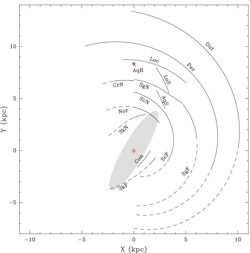
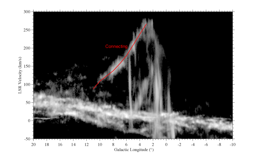
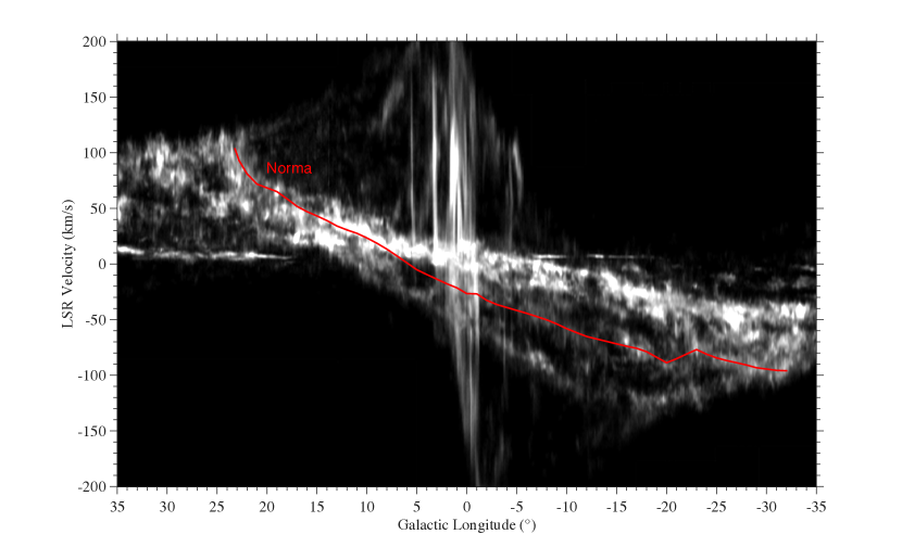
We used the fits of log-periodic spiral shapes to arm segments (slightly updated with some unpublished data) from the values summarized in Reid et al. (2014) to define the location of each arm segment (see Fig. 1). For any given Galactic longitude, we calculated the arm’s Galactocentric radius and azimuth, and , and the heliocentric distance, , and combined this information with the arm trace, to generate complete 6-parameter information, , for all arm segments. For the Aquila Spur, Aquila Rift, and Connecting arm, distances were estimated from only one or two parallaxes using simple linear forms. The information for 20 arm segments are currently used by the program, and we plan to update these and add new arm segments when more parallax data is available.
We calculate a distance PDF, based on spiral arm information, as the product of the probability density of distance to arm segments, based on models fitted to parallax data and other information, and the probability of association with those arm segments:
where indicates prior information on the locations of spiral arm segments, as well as Galactic (, , rotation curve) and Solar Motion (, ) parameters. We assign the probability that a source resides in the arm segment as follows:
where , , and are the minimum deviations in longitude, latitude, and velocity of the source from the center of the trace for the spiral arm, respectively, and , , and are their expected dispersions.
The in-plane and out of plane dispersions are given by and , respectively, where and are the in-plane and out of plane widths (Gaussian ) of an arm, and is the angle between the tangent to the arm and a ray from the Sun through the target source. The term accounts for the increased “effective” width of the arm owing to its orientation with respect to its closest approach to the target ray. Since real arms curve over kpc-scale lengths, we truncate above a value of 10.
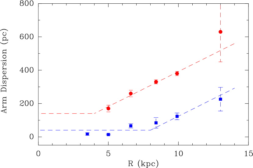
Both and can be a function of Galactocentric distance. Reid et al. (2014) found that spiral arm width increases with Galactocentric radius, , with a slope of 42 pc kpc-1 for kpc. Rather than extrapolate this to zero width near , we adopt kpc for kpc and constant at kpc in the central 4 kpc as shown in Fig. 2. In order to estimate the -width, we grouped the same parallax data by spiral arm and calculated the standard deviations about their mean offsets in . These are also plotted in the figure. The -widths are consistent with increasing for kpc with the same slope as for the in-plane widths, and we adopt a simple broken-linear relation kpc for kpc and 0.04 kpc inside of 8 kpc. Finally, we set , which is the expected Virial 1-dimensional speed difference for the target and a giant molecular cloud used to define the spiral arm trace. We adopt km s-1 , which is appropriate for M⊙ within pc.
In order to calculate , we generate an array of “trial” source distances, , and calculate the minimum separation of the source from a given arm segment model, both in the Galactic plane, , and out of the plane, . Then for the arm,
where the arm in-plane and z-widths are and . Note, we include the “normalization” terms, and , preceding the exponentials, since they vary with distance.
Since the sum of the probabilities of association with arms
can be small, we add a uniform background probability that allows for the possibility of a missing arm segment in our model and to some extent interarm sources (but see Section 5 for caveats). A user-adjustable parameter, from , determines the maximum weighting of the spiral arm associations relative to the background probability. When normalizing the PDF, we set the total background probability (i.e., integrated over distance) to be . Thus, for example, if , indicating zero probability of the target being associated with spiral arms, then the background probability would integrate to unity, regardless of the value assigned to . However, if , indicating a high probability that the source can be assigned to one or more arms, then the spiral arm PDF will be downweighted such that the background probability density would integrate to . The program defaults to .
2.2 Kinematic Distance PDF
The kinematic distance PDF, Prob, is generated for a given distance based on the velocity difference between the observed value and that expected from the rotation of the Galaxy. First, we calculate a “revised LSR velocity” to allow for differences between the Standard Solar Motion (which defines LSR velocities) and more recent estimates. We convert LSR to the Heliocentric velocities by removing the IAU Standard Solar Motion of 20 km s-1 toward R.A.=, Dec.=30∘ (in 1900 coordinates), which when precessed to J2000 give Cartesian Solar Motion components of (,,)=(10.27,15.32,7.74) km s-1 . Then we calculate the revised LSR velocity by applying (user-supplied) updated (,,) values. Interestingly, the IAU recommended values are surprisingly close to what could be considered today’s best values, and for simplicity the results in this paper adopt the IAU values.
Next, we obtain the velocity difference, , between the revised LSR velocity and that expected from the rotation of the Galaxy. Rather than use a simple linear rotation curve, we adopt the “Universal” rotation curve formulation of Persic, Salucci & Stell (1996) as implemented by Reid et al. (2014) (see their Figure 4 and Table 5 for details). This formulation is well motivated by observations of other galaxies, and it produces a nearly flat curve for Galactocentric radii kpc and slower rotation for sources inside that radius, in agreement with parallax and proper motion results.
Assuming an individual star in a high-mass star forming region has a random (Virial) motion of km s-1 in one dimension, we calculate the distance PDF via
where . We have used the Sivia & Skilling (2006) “conservative formulation” for the distance PDF, because it admits much higher probability for large deviations from the kinematic distance than would a Gaussian distribution. This is critical as it better approximates the true probability density from kinematic information, which can have large systematic errors owing to significant peculiar motions. See Section 3 for an example of an aberrant kinematic distance. Note that by directly generating a PDF, we have avoided calculating a traditional “kinematic distance,” which can have many complications when a velocity uncertainty is allowed.
For some sources, one may have prior information on the probability that the source is beyond the tangent point, near the far distance. For example, if H I absorption is seen toward an H II region with speeds exceeding that of the region by km s-1 , one can be fairly confident that the source distance is past the tangent point. (Although, there are places in the Galaxy where hydrogen gas has large non-circular motions that can lead to anomalous absorption velocities.) A user-supplied parameter, , giving the prior probability (from 0 to 1) that the source is at the far distance, is used to weight the near and far PDFs before they are summed and normalized. When no such prior information is available, , and both near and far kinematic distance PDFs are given equal weight.
2.3 Galactic Latitude PDF
A source’s Galactic latitude, , is a direct indicator of distance, independent of spiral arm association, since the is taller and narrower for a more distant source than for a near one. From Bayes’ theorem, the distance PDF can be calculated from
Neither nor introduce distance terms and converting from latitude to -height gives
Since and for a Gaussian distribution in , we find
The above formula is valid for a flat Galaxy. Allowing for a Galactic warp, we replace in the above relation with the difference, , between a source’s Galactic height and a model of the Galaxy’s warp. Rather than adopt a mathematical formula for warping, we use the spiral arm traces and calculate the -height of each arm segment at the intersection of the arm with a ray from the Sun through a target source position. At any given distance from the Sun, we then estimate the -height of the Galactic “plane” by interpolating (or extrapolating) linearly between () pairs of arm-warp parameters. Typically, we obtain 2 or 3 such ()-pairs in the and quadrants and 4 to 6 pairs in the quadrant. In order to evaluate the PDF, we use the broken-linear relation for presented in Section 2.1
2.4 Parallax Sources PDF
Sources with measured parallaxes have provided most of the information used to fit segments of spirals that are included in our prior knowledge (I), although other information (such as tangent-point longitudes) can be included in the models. However, adopting a log-periodic spiral model for arm segments kpc in length can be a simplification, and there is residual information in the parallax measures (e.g., star formation substructure and deviation of the real arm from the mathematical model) which we would like to use. So, we calculate a distance PDF based on association of the target source with a parallax source, Prob, as the product of the probability of distance given a parallax source, determined by its parallax accuracy, times the probability of association, given information for both the target and the parallax source. Summing over parallax sources gives
We quantify the association of a target source with a parallax source by calculating the probability that they reside within the same giant molecular cloud (GMC), based on the separations in linear distance in longitude () and latitude () and in velocity ():
where we set the expected 1-dimensional separation of two sources within a GMC to be kpc and the expected separation in line-of-sight velocity to be km s-1 .
For the source with measured parallax, , we calculate
where for a given distance , . Note, since what is measured is parallax, not distance, we have employed in the PDF calculation. Owing to the possibility of multiple parallax sources (possibly from different spiral arms) having similar values as the target source, we limit the impact of this probability term by adding a constant background probability density to based on the cumulative weight of the parallax matches:
A user-adjustable parameter, from , determines the maximum weighting of the parallax source association relative to the background probability. When normalizing the PDF, we set the total background probability integrated over distance to be . (See the discussion in Section 2.1.) In light of the partial correlation of individual parallax source information with that in the spiral arm model, the program defaults to a moderately-low weighting of this information by setting .
3 Example Distance PDFs
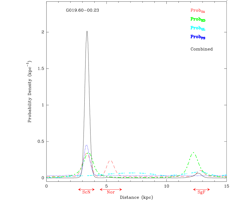
We present examples of the distance PDFs for sources in the and Galactic quadrants. G019.6000.23 is a star formation water maser at km s-1 from the Valdettaro et al. (2001) catalog and its distance PDF is shown in Fig. 3. This source was found to have a high probability of association with the near portion of the Scutum arm at a distance of 3.3 kpc and lower probabilities of association with the Norma arm at 5.3 kpc and the far portion of the Sagittarius arm at 12.9 kpc. Both the near kinematic distance and the association with a parallax source (G018.87+00.05) strongly favor the near Scutum arm distance. Combining all information, G019.6000.23 is estimated to be at a distance of kpc in the near portion of the Scutum arm with an integrated probability of 95% (and a 5% probability at kpc in the far portion of the Sagittarius arm).
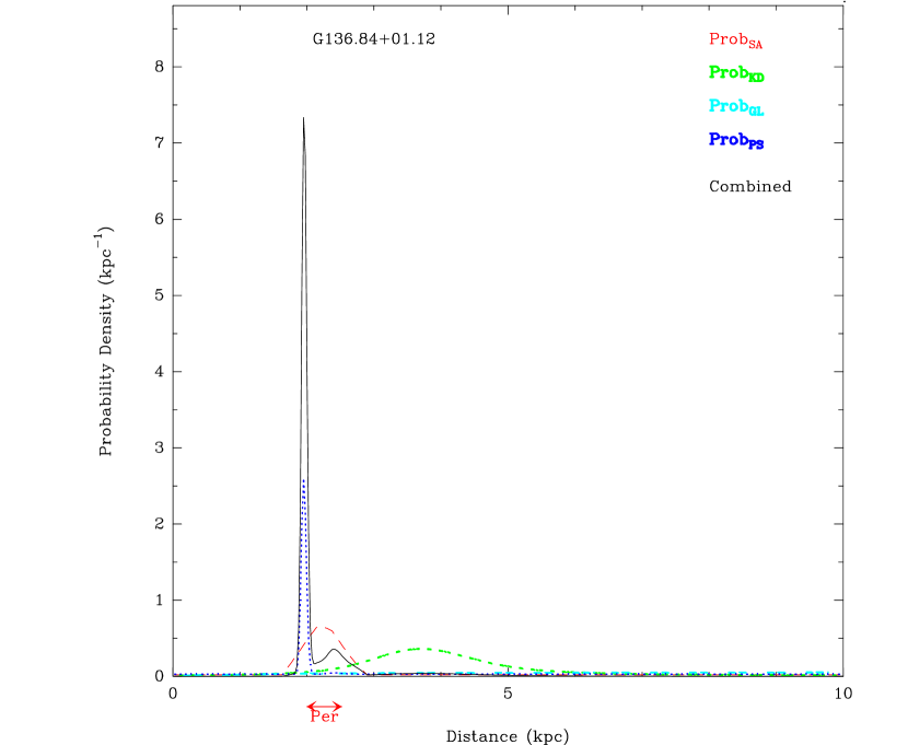
G136.84+01.12 is a 6.7 GHz methanol maser source at km s-1 in the Pestalozzi, Minier & Booth (2005) catalog, and its distance PDF is shown in Fig. 4. This source has a very high probability of association with the Perseus spiral arm (which crosses the source’s longitude at a distance of kpc). It may be associated with a giant molecular cloud containing the parallax source (G133.95+1.05) near the inner edge of the arm. The kinematic distance for G136.84+01.12 is 3.7 kpc, which, if correct, would place it in the Outer spiral arm. However, this portion of the Perseus arm is well known for kinematic anomalies, and the program correctly recognizes that the source values are inconsistent with Outer arm values. This is an example of the utility of a non-Gaussian PDF (see Section 2) for kinematic distances, as it accommodates such anomalies. The program favors a distance of kpc (based on the very accurate parallax to a nearby source) over a slightly greater distance of kpc (from the arm mid-line), as is apparent from an examination of the PDF.
4 Comparisons with Other Distance Estimates
A common method to estimate distances to Galactic sources of star formation is to use kinematic distances, augmented by H I absorption spectra to resolve the near/far ambiguity for sources within the Solar circle. Recently, Anderson et al. (2012) discovered large numbers of H II regions in the 1st quadrant, and for most they resolved the distance ambiguity via H I absorption. They found 62 sources that could be confidently (“A-grade”) placed at the far kinematic distance. Using our Bayesian approach with no prior information to resolve the near/far ambiguity (i.e., ), we were able to assign distances with 90% or greater probability for 34 of these sources. Of these sources, there was agreement between the H I absorption and our technique as to the resolution of the near/far distance ambiguity for all but six sources.
The techniques disagree for two sources near 19∘ longitude. For G018.324+0.026 and G019.6620.305, the Bayesian approach finds a significantly more probable association with the near portion of the Scutum arm at a distance of 3.4 kpc than with the far portion of the Sagittarius arm at 13 kpc. Similarly, we find G029.007+0.076 is likely associated with the near portion of the Scutum arm at a distance of kpc, whereas at the far kinematic distances of kpc there are no probable arm associations. If these sources are at the distances suggested by our Bayesian program, then they are near the end of the Galactic bar and may have significant non-circular motions, which could confuse distances based on kinematics and H I absorption.
For the remaining three sources (G032.2720.226, G034.041+0.053 and G034.133+0.471) we find them likely associated with the near portion of the Sagittarius arm at kpc rather than at the far kinematic distance of kpc. Note that along our line of sight toward longitude ∘ there may be gas with anomalous velocities owing to interaction with the supernova remnant W 44 (centered at () = () with a radius of 06) or with winds from its precursor.
Even though our program suggests a near distance for these six sources with greater than 90% probability, that still leaves a non-negligible probability for an alternative distance. All in all, we conclude that when a source can be assigned to a spiral arm with high probability, there is generally good agreement between our Bayesian approach and using H I absorption to resolve the near/far distance ambiguity.
5 The Milky Way’s Spiral Structure
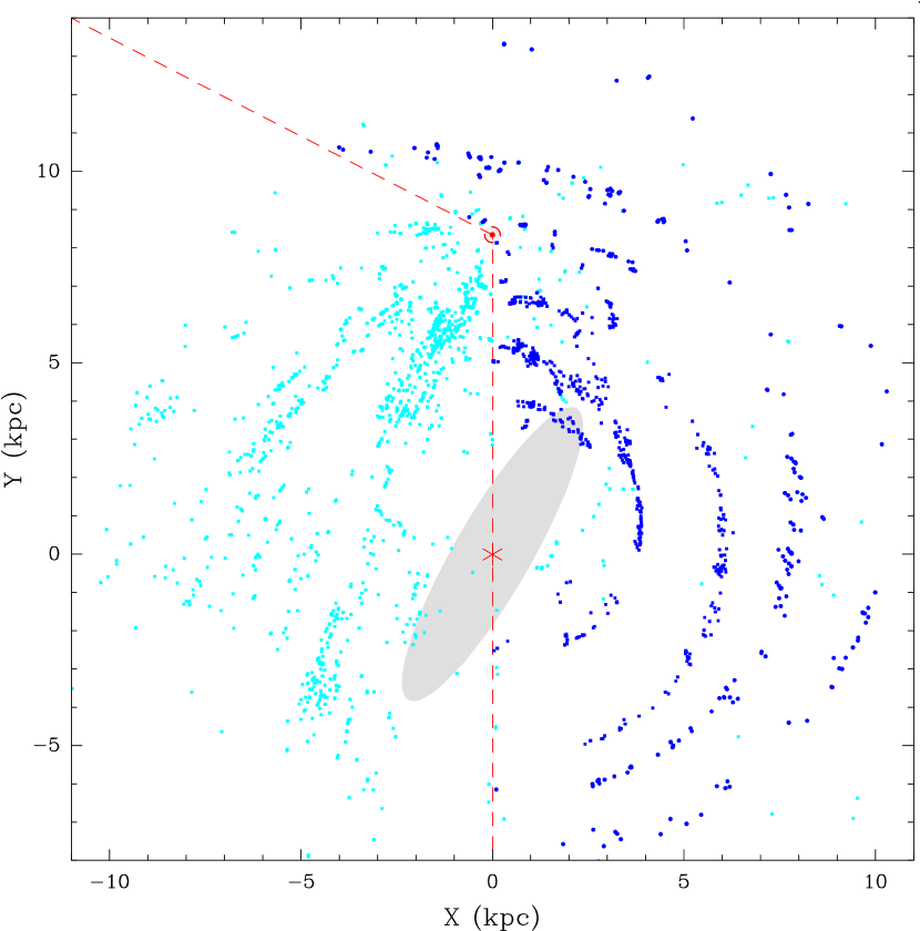
One application of our Bayesian distance estimation program is to generate a “plan view” (i.e., a projected view from high above the plane) of the spiral structure of the Milky Way. The left panel of Fig. 5 shows the locations of HMSFRs, assembled by combining catalogs of water (Valdettaro et al., 2001) and methanol (Pestalozzi, Minier & Booth, 2005) masers, HII regions (Anderson et al., 2012), and “red” MSX sources (Urquhart et al., 2014) sources. The distance to each source was determined from the component fitted to the combined distance PDF that had the greatest integrated probability. On the right-hand portion of this figure, where spiral arm locations are established by parallaxes, approximately 90% of the catalog sources are found to be associated with a spiral arm (indicated by the dark blue dots); the remaining approximately 10% probably represent interarm star formation (indicated by the light cyan dots). Since we do not yet have sufficient parallax measurements to locate spiral arms in the southern hemisphere (left-hand portion this figure), distance estimation there is based only on kinematics and latitude. The limitations of kinematic distances, including being multi-valued in the 4th quadrant and having variable sensitivity to non-circular motion, blur the spiral structure in this part of the Milky Way.
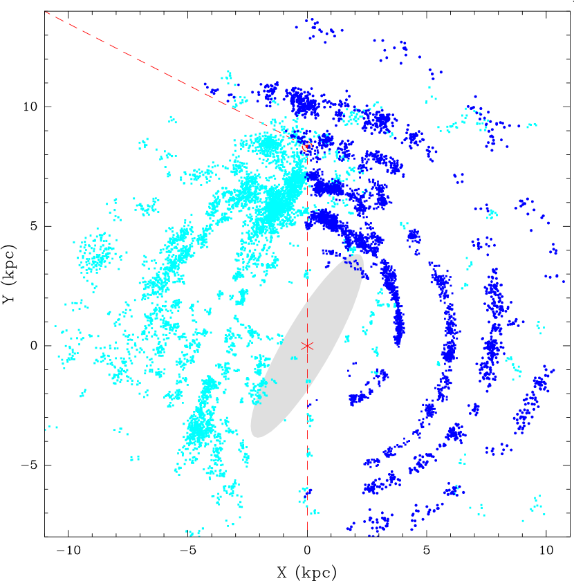
In the right panel of Fig. 5 we present a visualization of the Milky Way. For each catalog source we “sprinkle” five dots to simulate multiple sites of star formation in each giant molecular cloud. These dots were shifted from the catalog source location by adding Gaussianly distributed shifts with pc along each axis. The visualization suggests a clumpy spiral structure with depressions or gaps in massive star forming regions. The dearth of points in the Perseus arm between Galactic longitudes of 50∘ to 80∘, pointed out by Zhang et al. (2013) based on the lack of parallax sources, is apparent, even though the Bayesian distance estimation has no bias against portions of a spiral arm. The Outer and Sagittarius arms also show two or more gaps, several kpc in length.
The assumptions that go into, and the limitations of, Fig. 5 deserve discussion. Firstly, the accuracy of this figure directly depends on the locations of spiral arms, based on parallax results. Currently, the location of the Outer arm at Galactic longitudes , the Perseus and Sagittarius arms at longitudes , and the Scutum arms at longitudes are extrapolations based on pitch angles fitted to parallax sources at greater longitudes. Since spiral arms may have pitch angles that vary with azimuth (Honig & Reid, 2015), distances to sources in the extrapolated longitude ranges should be considered tentative, pending more parallax data.
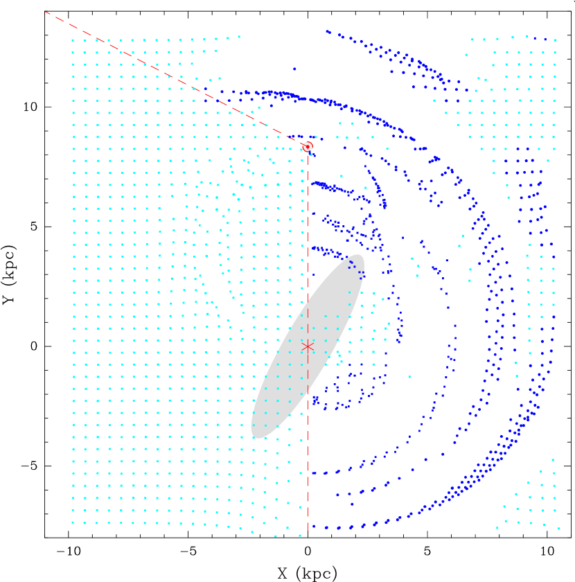
Secondly, even though we include a flat (non-zero) background probability density in the spiral arm PDF (see Section 2.1 for details), including in the combined distance PDF will “pull” peaks of combined probability density toward an arm center. To demonstrate this, we generated a uniform grid of sources that follow circular Galactic orbits, and estimate distances to these test sources. In order to simplify this demonstration, the test sources were placed exactly in the Galactic plane and the Galactic latitude, , and parallax source, , contributions to the combined distance PDF were ignored. The results of this uniform grid test are shown in Fig. 6. In regions of this uniform mock “Galaxy,” where spiral arm information is lacking, the grid is reasonably well preserved. However, where the spiral arm information exists and is used in the combined distance PDF, the results are biased to arms. This highlights the effects of the assumption made in the Bayesian distance estimation method that sources whose values are similar to the values of a known spiral arm segment probably are in that arm. Therefore, one should not use this method for sources that are not, or only weakly, associated with spiral structure, such as populations of old stars or diffuse gas.
This work was partially funded by the ERC Advanced Investigator Grant GLOSTAR (247078).
Facilities: VLBA, VERA, EVN
References
- Anderson et al. (2012) Anderson, L. D., Bania, T. M., Balser, D. S. & Rood, T. 2012 ApJ, 754, 62
- Benjamin (2008) Benjamin, R. A. 2008, in “Massive Star Formation: Observations Confront Theory,” ASP Conference Series, Vol. 387, eds. H. Beuther, H. Linz & Th. Henning, p. 375
- Blitz & Spergel (1991) Blitz, L. & Spergel, D. N. 1991, ApJ, 379, 631
- Choi et al. (2014) Choi, Y. K., Hachisuka, K., Reid, M. J., et al. 2014, ApJ, 790, 99
- Cohen et al. (1980) Cohen, R. S., Cong, H., Dame, T. M. & Thaddeus, P. 1980, ApJ, 239, L53
- Dame et al. (1986) Dame, T. M., Elmegreen, B. G., Cohen, R. S. & Thaddeus, P. 1986, ApJ, 305, 829
- Dame & Thaddeus (2008) Dame, T. M. & Thaddeus, P. 2008, ApJ, 683, L143
- Ellsworth-Bowers et al. (2013) Ellsworth-Bowers, T. P., Glenn, J., Rosolowsky, E. et al. 2013, ApJ, 770, 39
- Hachisuka et al. (2015) Hachisuka, K., Choi, Y. K., Reid, M. J., et al. 2015, ApJ, 800, 2
- Honma et al. (2012) Honma, M., Nagayama, T., Ando, K. et al. 2012, PASJ, 64, 136
- Honig & Reid (2015) Honig, Z. N. & Reid, M. J. 2015, ApJ, 800, 53
- Jackson et al. (2006) Jackson, J. M., Rathborne, J. M., Shah, R. Y. et al. 2006, ApJS, 163, 145
- McClure-Griffiths et al. (2012) McClure-Griffiths, N. M.; Dickey, J. M., Gaensler, B. M. et al. 2012, ApJS, 199, 12
- Persic, Salucci & Stell (1996) Persic, M., Salucci, P. & Stel, F. 1996, MNRAS, 281, 27
- Pestalozzi, Minier & Booth (2005) Pestalozzi, M. R., Minier, V., Booth, R. S. 2005, A&A, 432, 737
- Reid et al. (2009) Reid, M. J., Menten, K. M., Zheng, X. W. et al. 2009, ApJ, 700, 137
- Reid et al. (2014) Reid, M. J., Menten, K. M., Brunthaler, A. et al. 2014, ApJ, 783, 130
- Sato et al. (2014) Sato, M., Wu, Y. W., Immer, K., et al. 2014, ApJ, 793, 72
- Sivia & Skilling (2006) Sivia, D. & Skilling, J. 2006, Data Analysis: A Bayesian Tutorial (2nd ed.; New York, Oxford Univ. Press), 168
- Stil et al. (2006) Stil, J. M., Taylor, A. R., Dickey, J. M. et al. 2006, AJ, 132, 1158
- Urquhart et al. (2014) Urquhart, J. S., Figura, C. C., Moore, T. J. T., Hoare, M. G., Lumsden, S. L. et al. 2014, MNRAS, 437, 1791
- Valdettaro et al. (2001) Valdettaro, R., Palla, F., Brand, J., et al. 2001, A&A, 368, 845
- Weaver (1970) Weaver, H. 1970, IAU Symposium 38, “The Spiral Structure of Our Galaxy”, Eds. W. Becker & G. I. Contopoulos, (Dordrecht, Reidel), p.126
- Wu et al. (2014) Wu, Y. W., Sato, M., Reid, M. J., et al. 2014, A&A, 566, 17
- Xu et al. (2013) Xu, Y., Li, J. J., Reid, M. J., et al. 2013, ApJ, 769, 15
- Xu et al. (2016) Xu, Y., Reid, M. J., Dame, T. M. et al. , in preparation
- Zhang et al. (2013) Zhang, B., Reid, M. J., Menten, K. M. et al. (2013), ApJ, 775, 79
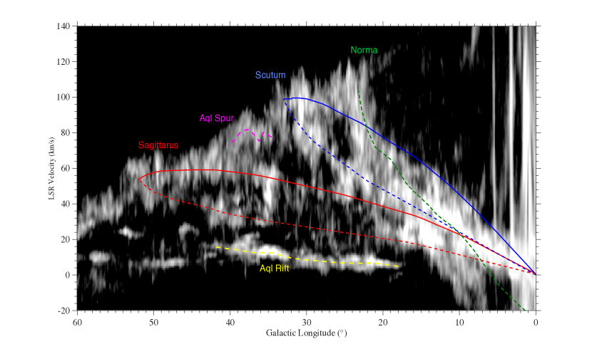
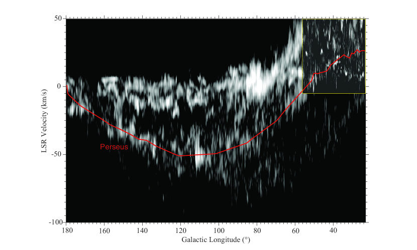
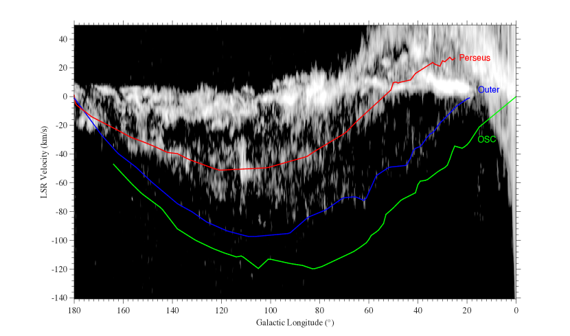
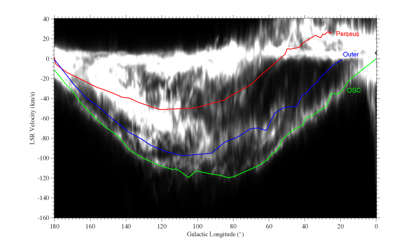
6 Appendix
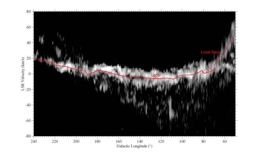
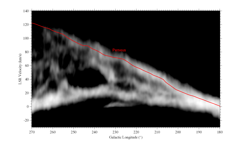
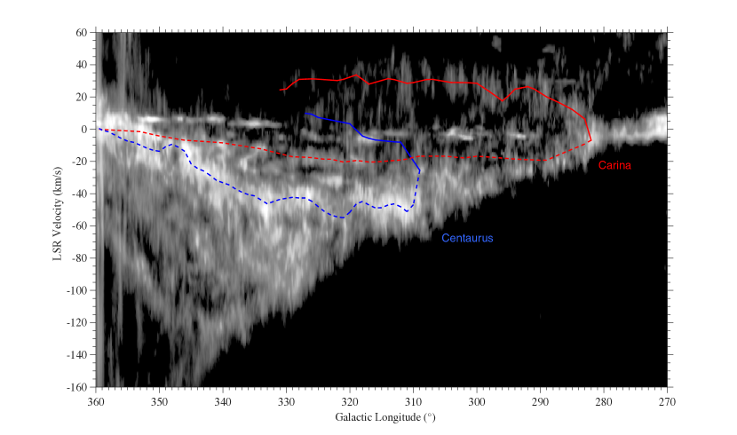
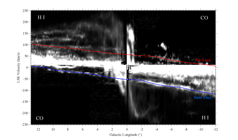
In Figs. 7–16 we optimally display and trace the numerous arcs and loops in HI 21 cm and CO diagrams that have long been recognized as Galactic spiral arms (Weaver, 1970; Cohen et al., 1980). These features were used by the BeSSeL Survey to assign high mass star forming regions with measured parallaxes to spiral arms, and they can likewise be used for any spiral arm tracer with a measured velocity by our program. While some of the features are very obvious (e.g., the Perseus arm in the second quadrant; Fig. 8), others are less so owing to blending with unrelated emission either at the opposite kinematic distance in the inner Galaxy or at other latitudes. For instance, the Far 3-kpc Arm (Dame & Thaddeus, 2008) can only be seen clearly in an diagram integrated over a very narrow range of latitude near the plane (see Fig. 14). Other features are not only narrow in latitude but are offset from the plane and may even vary in latitude as a function of both longitude and velocity (e.g., the Outer Scutum-Centaurus arm; Fig. 10). Details on how the diagrams were produced to best display each arm are given in the captions.
All of the spiral arm tracks, indicated by the colored lines in the figures, roughly correspond in shape and alignment with those expected for segments of logarithmic spiral arms, but we do not fit the features in that way, nor do we extrapolate or link up tracks in regions where they are not clearly seen. Rather, we run the tracks through the actual emission features that define the arms in longitude, latitude, and velocity. In some cases this results in a jaggedness that is slightly subjective, but they are the tracks of the actual spiral arms in the raw spectral-line data, and they are the structures that are now being located accurately in the Galaxy for the first time using maser parallaxes. How or whether these structures link up into a grand design spiral pattern is not relevant for the present purpose.