Topological mirror insulators in one dimension

Abstract

We demonstrate the existence of topological insulators in one dimension protected by mirror and time-reversal symmetries. They are characterized by a nontrivial $\mathbb{Z}_{2}$ topological invariant defined in terms of the “partial” polarizations, which we show to be quantized in presence of a 1D mirror point. The topological invariant determines the generic presence or absence of integer boundary charges at the mirror-symmetric boundaries of the system. We check our findings against spin-orbit coupled Aubry-André-Harper models that can be realized, e.g. in cold-atomic Fermi gases loaded in one-dimensional optical lattices or in density- and Rashba spin-orbit-modulated semiconductor nanowires. In this setup, in-gap end-mode Kramers doublets appearing in the topologically non-trivial state effectively constitute a double-quantum-dot with spin-orbit coupling.

I Introduction

The study of topological phases of matter is one of the most active research areas in physics. Triggered by the discovery of the quantum Hall effect in 1980Klitzing et al. (1980) and its theoretical explanation in terms of the topological properties of the Landau levels,Thouless et al. (1982); Kohmoto (1985) a plethora of topologically nontrivial quantum phases has been predicted theoretically and confirmed experimentally.Bernevig et al. (2006); König et al. (2007); Xia et al. (2009); Rasche et al. (2013); Pauly et al. (2015); Kane and Mele (2005); Liu et al. (2011); Lau and Timm (2013); Young et al. (2012); Liu et al. (2014); Wan et al. (2011); Huang et al. (2015) In particular, topological insulators and superconductors have been the subject of intensive research efforts.Moore (2010); Hasan and Kane (2010); Qi and Zhang (2011); Fu (2011) Unlike their topologically trivial counterparts, they exhibit protected surface or edge states inside the bulk excitation gap of the material. These topological boundary states are the prime physical consequence of the topology of the bulk band structure, which is encoded in a quantized topological invariant.Hasan and Kane (2010); Ryu et al. (2010)

Belonging to the symplectic class AII of the Altland-Zirnbauer (AZ) classification, time-reversal invariant topological insulators in two (2D) and three dimensions (3D) are characterized by a $\mathbb{Z}_{2}$ topological invariant. Primary examples of topologically nontrivial systems include HgTe/CdTe quantum wells in 2D,König et al. (2007) and Bi₂Se₃ in 3D.Xia et al. (2009) For one-dimensional (1D) systems, instead, the AZ scheme does not predict a similar topological invariant, and thus all insulating phases are expected to be topologically equivalent.

In the context of recent findings of novel topological states of matter protected by additional continuous symmetries,Chiu et al. (2013); Shiozaki and Sato (2014); Hughes et al. (2011); Lau et al. (2015); Zhang et al. (2013); Ueno et al. (2013); Slager et al. (2012) we show here that a crystalline symmetry, namely mirror symmetry, leads to a class of 1D time-reversal invariant topological insulators beyond the standard AZ classification of topological insulators. Using the concept of partial polarizations, we demonstrate that the concomitant presence of mirror and time-reversal symmetry allows the definition of a $\mathbb{Z}_{2}$ topological invariant. A nonzero value of this invariant defines a one-dimensional topological mirror insulator, which hosts an odd number of integer electronic end charges. We will present an explicit tight-binding model built upon the well-known Aubry-André-Harper (AAH) model realizing this novel topological state of matter. By calculating its topological invariants, we determine the phase diagram of the system. Moreover, we consider energy spectra of finite chains and calculate the corresponding values of the end charges to explicitly confirm the topological nature and the bulk-boundary correspondence. We further study the effect of weak on-site disorder. We find that the topological features are robust as long as mirror symmetry is preserved on average. We finally show that a particular realization of this model can be achieved in cold atomic Fermi gases loaded in 1D optical lattices and in semiconductor nanowires with gate-modulated Rashba spin-orbit coupling.

II $\mathbb{Z}_{2}$ Topological Invariant

We start out by considering a generic system of spin one-half fermions in a 1D crystalline potential with time-reversal symmetry $\Theta$. In addition, we will consider the crystal to be mirror symmetric with respect to a 1D mirror point. The Bloch Hamiltonian of such a system ${\cal H}(k)$, where $k\in(-\pi,\pi]$ with the lattice constant set to unity, then inherits the two following symmetry constraints:

$$\Theta{\cal H}(k)\Theta^{-1}={\cal H}(-k),\ \ {\cal M}{\cal H}(k){\cal M}^{-1}={\cal H}(-k),$$ (1)

where ${\Theta}=(\mathbb{1}\otimes is^{y})K$ is the antiunitary time-reversal operator, while ${\cal M}={\cal I}\otimes is^{x}$ is the unitary operator corresponding to the operation of reflection with respect to the 1D mirror point. Without loss of generality, we assume the latter to be in the $\hat{x}$ direction. In addition, the $s^{i}$ are the usual Pauli matrices acting in spin space, while ${\cal I}$ acts only on the spatial degrees of freedom and thus corresponds to spatial inversion. For this representation of the symmetry operations, we have that $[\Theta,{\cal M}]=0$, ${\Theta}^{2}=-1$ as required for spin one-half fermions, and ${\cal M}^{2}=-1$, since spatial inversion must square to the identity, i.e., ${\cal I}^{2}=1$.

The Berry phaseZak (1989) $\gamma$ associated with the 1D Bloch Hamiltonian ${\cal H}(k)$ defines the charge polarization per unit cellFu and Kane (2006) via $P_{\rho}=\gamma/2\pi$, with the electronic charge set to unity. Because of the intrinsic $2\pi$ ambiguity of the Berry phase, $P_{\rho}$ is defined up to an integer and can generally assume any value in between. However, this assertion does not hold true for a 1D insulator with a 1D mirror point. To show this, we first exploit the time-reversal symmetry of the system and consider the partial polarizations introduced by Fu and Kane.Fu and Kane (2006) Due to Kramers’ theorem every Bloch state at $k$ comes with a time-reversed degenerate partner at $-k$. Hence, all occupied bands can be divided into two time-reversed channels. The partial polarization $P^{s}$ is then just the charge polarization of channel $s=\mathrm{I,II}$ such that $P_{\rho}=P^{I}+P^{II}$. Using the symplectic time-reversal symmetry for spin one-half fermions, it is possible to show that $P^{I}=P^{II}$ modulo an integer [c.f. Appendix A and Ref. Fu and Kane, 2006].

The crux of the story is that in presence of mirror symmetry with the symmetry operator ${\cal M}$ commuting with the time-reversal symmetry operator, the partial polarizations satisfy $P^{s}=-P^{s}\>\mathrm{mod}\,1$ [c.f. Appendix A]. Henceforth, $P^{s}$ can only assume the two distinct values $0$ and $1/2$ (modulo an integer). The consequence of this result is twofold. First, it follows that the charge polarization $P_{\rho}$ of a 1D insulator with a 1D mirror point is an integer quantity. Second, the quantized nature of the partial polarization allows to define a $\mathbb{Z}_{2}$ topological invariant $\nu=2P^{s}\mathrm{mod}\,2\equiv 0,1$. This gives rise to two topologically distinct states that cannot be adiabatically connected without closing the bulk energy gap or breaking the defining symmetries. Using the $U(2N)$ invariant form of the partial polarization,Fu and Kane (2006) where $2N$ is the number of occupied energy bands, the topological invariant explicitly reads:

$$\nu:=\frac{1}{\pi}\bigg{[}\int_{0}^{\pi}dk\>\mathcal{A}(k)+i\,\log\Big{(}\frac{\mathrm{Pf}[w(\pi)]}{\mathrm{Pf}[w(0)]}\Big{)}\bigg{]}\,\mathrm{mod}\,2,$$ (2)

where $\mathcal{A}(k)=i\sum_{n\,\mathrm{occ.}}\langle u_{k,n}|\partial_{k}|u_{k,n}\rangle$ is the Berry connection of all occupied bands and we introduced the $U(2N)$ matrix $w_{\mu\nu}(k)=\langle u_{-k,\mu}|\Theta|u_{k,\nu}\rangle$ which is antisymmetric at $k=0,\pi$ and thus characterized by its Pfaffian $\mathrm{Pf}(w)$.

The quantization of the partial polarization in one-dimensional systems with a mirror point has a direct physical consequence. The charge polarization of a system is indeed directly connected to the accumulated bound charge at its surfaces.King-Smith and Vanderbilt (1993) For a one-dimensional system the end charge $Q$ is simply related to the polarization $P$ by $Q\,\mathrm{mod}\,1=P$. Since the partial polarization $P^{\mathrm{I}}$ is just the usual polarization associated with one of the time-reversed channels, we can assign a partial bound charge to this channel, which is proportional to $P^{\mathrm{I}}$. With two identical time-reversed channels, the total bound charge per end is then

$$Q\,\mathrm{mod}\,2=2P_{\mathrm{I}}=\nu.$$ (3)

This establishes a direct connection between the number of bound charges and the $\mathbb{Z}_{2}$ invariant $\nu$. In particular, systems for which $\nu=1$ are topological mirror insulators: they are characterized by the presence of an odd number of integer-valued electronic end charges at the mirror symmetric boundaries of the system [c.f. Refs. King-Smith and Vanderbilt, 1993; van Miert et al., 2016]. This is the central result of this paper.

A few remarks are in order. First, we emphasize that the quantities in Eq. (2) require a continuous gauge. Such a gauge can be straightforwardly constructed from numerically obtained eigenstates [c.f. Appendix B]. Second, we note that the $\mathbb{Z}_{2}$ invariant of Eq. 2 cannot be determined from the knowledge of the electronic wavefunctions only at the time-reversal invariant momenta, as it occurs for crystalline topological insulators in 2D and 3D. Eq. 2 requires the knowledge of the wavefunctions in the entire BZ. This also implies that for a topological phase transition, that occurs via a closing and reopening of the 1D bulk gap at momentum $q$, $q$ is in general not a high-symmetry point in the BZ.

We finally point out that the existence of our $\mathbb{Z}_{2}$ topological invariant does not contradict the AZ classification of topological insulators and superconductors,Zirnbauer (1996); Altland and Zirnbauer (1997); Heinzner et al. (2005); Schnyder et al. (2008); Kitaev (2009); Ryu et al. (2010), which does not take into account the point-group symmetries of the system. In the absence of mirror symmetry, the partial polarizations of a 1D system with time-reversal symmetry are indeed no longer quantized, and therefore $\nu$ does not represent an invariant. The existence of 1D topological mirror insulators is instead in agreement with the recent extensions of the original AZ classification taking into account point-group symmetries,Lu and Lee (2014); Chiu et al. (2013); Shiozaki and Sato (2014) in particular with Refs. Shiozaki and Sato, 2014 and Chiu et al., 2013 which predict that mirror-symmetric 1D systems in principle allow for a $\mathbb{Z}_{2}$ invariant. In this respect, it must be pointed out that certain types of translational-symmetry breaking terms, such as charge-density waves, can turn the system into a trivial insulator, similar to weak topological insulators in 3D. From this point of view, a topological mirror insulator can be viewed as a realization of a low-dimensional, weak topological insulator.

Figure 1: (color online) Phase diagram and spectra of the spin-orbit coupled AAH model with $\alpha=\gamma=1/2$ (dimerization), $\beta=1/4$, $V_{0}=0$, $\lambda_{0}=0.5t_{0}$, $\delta\lambda=-0.3t_{0}$, $\phi_{t}=\phi_{\lambda}=\pi$: (a) half-filling phase diagram of the bulk for $\phi_{V}=-\pi/4$. The value of the $\mathbb{Z}_{2}$ invariant $\nu$ is indicated by pixel color. Note that it only assumes two distinct values, $0$ and $1$. (b-d) Bulk band structures for $\delta V=0.5t_{0}$ and fixed $\delta t$ with (b) $\delta t=-0.1t_{0}$, (c) $\delta t=\delta t_{c}\approx 0.025$, (d) $\delta t=0.1t_{0}$. The band structures correspond to systems along the arrow in (a). Note that the half-filling bulk energy gap closes away from the time-reversal invariant points $k=0$ and $\pi$.

III Spin-orbit coupled Aubry-André-Harper models

We are now going to present an explicit model that features a 1D topological mirror insulating phase. In particular, we will consider the following tight-binding Hamiltonian for spin-$1/2$ electrons on a 1D lattice

$$\mathcal{H} = \sum_{j,\sigma}[t_{0}+\delta t\cos(2\pi\alpha j+\phi_{t})]\,c_{j+1,\sigma}^{\dagger}c_{j\sigma}$$ (4)

$${}+\sum_{j,\sigma}[V_{0}+\delta V\cos(2\pi\beta j+\phi_{V})]\,c_{j\sigma}^{\dagger}c_{j\sigma}$$

$${}+i\sum_{j,\sigma,\sigma^{\prime}}[\lambda_{0}+\delta\lambda\cos(2\pi\gamma j+\phi_{\lambda})]\,c_{j+1,\sigma}^{\dagger}s^{y}_{\sigma\sigma^{\prime}}c_{j\sigma^{\prime}}$$

$${}+\mathrm{h.c.}$$

This is a generalization of the famous Aubry-André-Harper (AAH) model.Harper (1955); Aubry and André (1980); Ganeshan et al. (2013); Lau et al. (2015) It contains harmonically modulated nearest-neighbor hopping, on-site potentials and spin-orbit coupling (SOC) with amplitudes $\delta t$, $\delta V$, $\delta\lambda$, phases $\phi_{t}$, $\phi_{V}$, $\phi_{\lambda}$, and periodicities $1/\alpha$, $1/\beta$, $1/\gamma$. For simplicity, we restrict the model to rational values of the periodicities. Moreover, $t_{0}$, $V_{0}$ and $\lambda_{0}$ are the bond and site independent values of hopping, potentials and SOC, the operators $c_{j\sigma}^{\dagger}$ ($c_{j\sigma}$) create (annihilate) an electron with spin $\sigma$ ($\sigma=\uparrow,\downarrow$) at lattice site $j$, and the $s^{i}$ are Pauli matrices. The Hamiltonian of Eq. 4 possesses time-reversal symmetry whereas mirror symmetry is present only for specific values of the phases $\phi_{t}$, $\phi_{V}$ and $\phi_{\lambda}$. For the computation of band structures and eigenstates we use exact numerical diagonalization. In the case of periodic boundary conditions, we exploit the translational symmetry of the system and work with the corresponding Bloch Hamiltonian in momentum space. For open boundary conditions, we take the real-space Hamiltonian with a finite number of unit cells. The $\mathbb{Z}_{2}$ invariant of Eq. (2) is calculated numerically using the aforementioned procedure to construct a continuous $U(2N)$ gauge from numerically obtained eigenstates [c.f. Appendix B].

Figure 2: (color online) Spectra of the spin-orbit coupled AAH model in a finite geometry for different $\phi_{V}$. Other parameters are $\alpha=\gamma=1/2$ (dimerization), $\beta=1/4$, $V_{0}=0$, $\delta V=0.5t_{0}$ $\lambda_{0}=0.5t_{0}$, $\delta\lambda=-0.3t_{0}$, $\phi_{t}=\phi_{\lambda}=\pi$: (a) $\delta t=-0.5t_{0}$, (b) $\delta t=0.5t_{0}$. States localized at the ends of the chain are highlighted in red. In addition, we display the Hall conductivities $\sigma$ in units of $e^{2}/h$ associated with each gap when $\phi_{V}$ is interpreted as an additional momentum variable.

We will consider the model in Eq. (4) with $\alpha=\gamma=1/2$, $\phi_{t}=\phi_{\lambda}=\pi$, $V_{0}=0$, and $\beta=1/4$. With this choice of parameters, the unit cell of our model Hamiltonian contains four lattice sites and the model preserves reflection symmetry for $\phi_{V}=-\pi/4$ and $3\pi/4$. This is a direct generalization of the model considered in Ref. Lau et al., 2015 to the spinful case. The model can be potentially realized using an ultracold Fermi gas loaded in a 1D optical lattice Bloch (2005); Aidelsburger et al. (2013); Cheuk et al. (2012); Wang et al. (2012), while the ensuing end states can be detected using time-of-flight measurements or optical microscopy.Mancini et al. (2015); Leder et al. (2016) We emphasize that while state-of-the-art technologies allow to create SOC terms explicitly breaking mirror symmetry,Zhai (2015); Liu et al. (2013) the rapid progress in the field can be expected to bring soon a much larger variety of SOC terms into reach.Zhai (2015); Campbell et al. (2011); Wall et al. (2016)

III.1 Phase diagram and in-gap end states

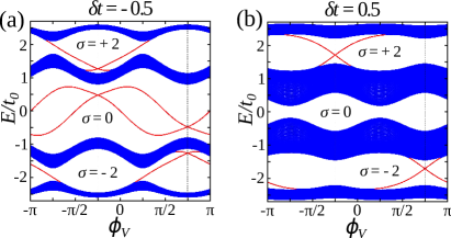
We first determine the phase diagram of our system with respect to the $\mathbb{Z}_{2}$ invariant $\nu$ of Eq. (2) for the half-filled system at $\phi_{V}=-\pi/4$, i.e., where the model has reflection symmetry. The phase diagram in the $\delta t$-$\delta V$ parameter space is shown in Fig. 1(a). We identify two phases which are separated by a parabolic phase boundary: a trivial phase with $\nu=0$ on the right side and a topological phase with $\nu=1$ on the left side. Similarly to the spinless version of the model,Lau et al. (2015) the bulk energy gap at half-filling closes at the topological phase transition.

Note that bulk band gap closing and reopening occurs away from the time-reversal invariant momenta, as is shown in Figs. 1(b-d). This is in contrast to other crystalline topological phases as pointed out in the previous section.

Moreover, the nontrivial topology of the model manifests itself through the appearance of characteristic in-gap end states. This is checked and demonstrated in Fig. 2 where we show the energy spectra of the AAH model under consideration with a finite number of unit cells and open boundary conditions. The phase shift $\phi_{V}$ of the on-site modulation is varied smoothly from $-\pi$ to $\pi$ thereby passing through the mirror-symmetric cases at $-\pi/4$ and $3\pi/4$. At these points, we find four degenerate in-gap end states at half filling provided we are in the nontrivial area of the phase diagram of Fig. 2(a). Away from the mirror-symmetric points the observed states are split into two degenerate pairs. The two-fold degeneracy remains since the model in Eq. 4 preserves time-reversal symmetry at all values of $\phi_{V}$. The half-filling end states are not encountered for parameters of the model for which we are in the trivial region of the phase diagram, as can be seen in Fig. 2(b).

Taking a different perspective, the appearance of end states at the $1/4$ and $3/4$ filling gaps can also be understood by interpreting the phase $\phi_{V}$ as the momentum of an additional artificial dimension. In this case, our model of Eq. 4 can be mapped to a dimerized Hofstadter modelHofstadter (1976); Ganeshan et al. (2013); Lau et al. (2015); Marra et al. (2015) for spinfull fermions with SOC in one direction only. Contrary to models investigated before,Cocks et al. (2012); Orth et al. (2013) the resulting model explicitly breaks the 2D time-reversal symmetry constraint $\Theta^{-1}{\cal H}(k,\phi_{V})\Theta\neq{\cal H}(-k,-\phi_{V})$, thereby allowing for insulating states with nonzero Chern numbers.Lau et al. (2015); Thouless et al. (1982); Kohmoto (1985) By calculating the Hall conductivities, we find that they are doubled with respect to the conventional spinless Hofstadter modelLau et al. (2015) indicating that the two spin channels of our model carry the same topological content. This, in turn, implies that the in-gap states at $1/4$ and $3/4$ filling, appearing in Fig. 2, correspond to the chiral edge states of a generalized Hofstadter model in a ribbon geometry. Furthermore, they correspond to insulating states with Hall conductivities $\pm 2$. On the contrary, the insulating phase at half-filling has zero Hall conductivity but displays two quartets of edge states in the topological phase originating from the 1D mirror-symmetric cuts [c.f. Fig. 2(a)]. We point out that these results, as a generalization of Ref. Lau et al., 2015, extend to arbitrary rational $\beta=p/q$ with $p$ and $q$ coprime.

III.2 Bulk-edge correspondence

We have shown that the appearance of electronic in-gap end states is characteristic of a topological mirror insulator. However, due to the absence of chiral symmetry, which would pin the end modes at the center of the gap, symmetry-allowed perturbations can push the end modes into the continuum of bulk states. Such perturbations could, for instance, be introduced by surface potentials.

Figure 3: (color online) Spectra and local charge densities of the mirror-symmetric, spin-orbit coupled AAH model with open boundary conditions and $\alpha=\gamma=1/2$, $\beta=1/4$, $V_{0}=0$, $\delta V=0.5t_{0}$, $\lambda_{0}=0.5t_{0}$, $\delta\lambda=-0.3t_{0}$, $\phi_{t}=\phi_{\lambda}=\pi$, $\phi_{V}=-\pi/4$, and a surface potential $V_{\mathrm{LR}}=0.6t_{0}$: (a) Topological phase with $\delta t=-0.5t_{0}$, (b) trivial phase with $\delta t=0.4t_{0}$. The main panels show the energy spectra with end states highlighted in red. The dashed line signifies the chemical potential $\mu$ used for the calculation of the local charge densities $\rho_{j}$. The latter are presented in the insets. In addition, we display the corresponding values of the electronic end charges $Q_{\mathrm{L}}$ and $Q_{\mathrm{R}}$.

We explicitly demonstrate the point above by adding a generic surface potential $\sum_{\sigma}V_{\mathrm{LR}}(c_{1\sigma}^{\dagger}c_{1\sigma}+c_{L\sigma}^{\dagger}c_{L\sigma})$ to our model with open boundary conditions, and analyzing the ensuing energy spectra. Again, we fix the on-site potential phase $\phi_{V}$ to $-\pi/4$ such that our model preserves mirror symmetry.

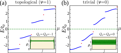
Without the surface potential, we observed two degenerate in-gap Kramers pairs at half filling in the topological phase [see Fig. 2(a)]. This picture changes if we switch on the surface potential $V_{\mathrm{LR}}$ [see Fig. 3(a)]. We observe that the end modes in the half-filling gap are pushed up into the conduction band, while another degenerate pair of Kramers doublets emerges from the valence band. However, the appearance of these states cannot be linked to the topological invariant of the system. In fact, these additional states occur both in the topological and in the trivial phases, as can be seen by comparing Figs. 3(a) and (b) at half-filling.

Having established that sufficiently strong symmetry-allowed edge potentials are detrimental for the occurrence of in-gap end modes, we now proceed to uncover the bulk-edge correspondence for 1D topological mirror insulators, i.e., the existence of an odd number of integer-valued electronic end charges.

We define the end charge of a system to be the net deviation of the local charge density close to the end from the average charge density in the bulk. Adopting the definition of Ref. Park et al., 2016, we calculate the left end charge $Q_{\mathrm{L}}$ as the limit of

$$\sum_{j}^{L}\Theta(l_{0}-j)(\rho_{j}-\bar{\rho})$$ (5)

for sufficiently large $l_{0}$. A similar definition is used for the right end charge $Q_{\mathrm{R}}$ with $\Theta(l_{0}-L+j)$. Here, $L$ is the length of the chain, $\Theta(x)$ is the Heaviside function and $l_{0}$ is a cut-off. $\rho_{j}=\sum_{\nu}^{N}|\psi_{\nu}(j)|^{2}$ is the local charge density of the ground state in units of $-e$ with the sum running over all $N$ occupied states $\psi_{\nu}$ up to the chemical potential $\mu$. The bulk charge density $\bar{\rho}$ is treated as a constant background that is fixed by the chemical potential. In particular, at half filling we have $\bar{\rho}=1$ corresponding to one electron per site.

The insets in Fig. 3 show the local charge densities of the finite AAH chains when the chemical potential $\mu$ is in the half-filling bulk energy gap above or below the end states. As expected, the local charge density oscillates around $1$ in the bulk. Moreover, in the topological phase there are large deviations from this value near the ends of the system indicating the presence of electronic end charges. On the contrary, there are no pronounced features in the trivial phase.

This is confirmed by explicit calculation of the end charges. In the topological phase [see Fig. 3(a)] we find $Q_{\mathrm{L}}=Q_{\mathrm{R}}=+1$ when $\mu$ is placed right above the topological end states. Leaving the two boundary states at each end unoccupied leads to an end charge of $-1$. Hence, there is a direct correspondence between end states and end charges. End states always come in degenerate pairs due to time-reversal symmetry. From this we see that, regardless of where we put the chemical potential in the bulk energy gap and regardless of how many pairs of degenerate Kramers pairs are present, the end charge will always assume an odd value in agreement with the general analysis of the previous section. More importantly, this is a robust feature that is not affected by the presence of surface potentials.

In contrast to that, in the trivial phase [see Fig. 3(b)] we find $Q_{\mathrm{L}}=Q_{\mathrm{R}}=0$ for a chemical potential above the trivial end states. Hence, only even values of end charges are possible. For instance, with the trivial states unoccupied we calculate end charge values of $-2$. In addition, the end charges no longer assume integer values if mirror symmetry is broken.

III.3 Effect of disorder

Figure 4: (color online) Effect of disorder in the half-filled, spinful AAH model with open boundary conditions and $\alpha=\gamma=1/2$, $\beta=1/4$, $t=-0.5t_{0}$ $V_{0}=0$, $\delta V=0.5t_{0}$, $\lambda_{0}=0.5t_{0}$, $\delta\lambda=-0.3t_{0}$, $\phi_{t}=\phi_{\lambda}=\pi$, and $\phi_{V}=-\pi/4$ (topological phase): (a) Disorder-averaged IPR $\langle I_{\psi}\rangle$ for bulk states and end states. (b) Disorder-averaged end charges $\langle Q_{\mathrm{L}}\rangle$ and $\langle Q_{\mathrm{R}}\rangle$ with the chemical potential right below the in-gap end states. Shown is the dependence on the standard deviation $\gamma$ of the random disorder potential.

We have considered the fate of the characteristic in-gap end states and of the topological end charges of a 1D mirror insulator under the influence of disorder. The topological nature of a 1D topological mirror insulator is protected by time-reversal and mirror symmetry. The latter is a spatial symmetry and is, in general, broken by disorder. However, recent studies on topological crystalline insulators have shown that their topological features are still present if the protecting symmetry is preserved on average.Shiozaki and Sato (2014) We will now demonstrate that this holds also for our class of systems. To show this, we model the the effect of disorder by adding a random nonmagnetic on-site potential to our model of the form $\sum_{j}W_{j}c_{j\sigma}^{\dagger}c_{j\sigma}$, where the $W_{j}$ are independent random variables subject to a Gaussian distribution with zero mean and standard deviation $\gamma$. The latter is a measure for the disorder strength.

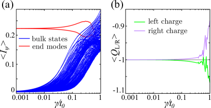
To analyze the effect of disorder on the end states we consider the expectation value of the inverse participation ratio (IPR), which is a quantitative measure of localization.Park et al. (2016); Pandey and Ortix (2016) The IPR of a given state $\psi$ is defined as $I_{\psi}=\sum_{j}^{L}|\psi(j)|^{4}$ with $|\psi(j)|^{2}$ being the weight of the state at site $j$. The IPR assumes values in the interval $(0,1]$. An IPR of $1$ corresponds to a perfectly localized state, whereas small values indicate a state equally distributed over the whole length of the system.

In Fig. 4(a) we present the IPR of occupied states for the finite, half-filled AAH chain of length $L=200$ averaged over $10^{3}$ random disorder configurations. The model parameters are chosen such that the disorder-free chain preserves mirror symmetry and is in the topological phase. We observe that the IPR of the topological end states stays nearly unaffected at a large value as long as the disorder is weak ($\gamma\lesssim 0.01t_{0}$). In contrast to that, the IPR of the bulk states is more than one order of magnitude lower. For stronger disorder the topological end modes are still well-localized, but their IPR starts to deviate from their previously constant value due to mixing with bulk states. However, this does not lead to a sizable decrease of the IPR due to the onset of Anderson localization. The latter also accounts for the substantial increase in the IPR of the bulk states.

In addition, in Fig. 4(b) we show the disorder-averaged values of the boundary charges $Q_{\mathrm{L}}$ and $Q_{\mathrm{R}}$ in the same setting. The chemical potential, which determines the number of occupied states, is set to be in the half-filling bulk energy gap such that the topological end states are unoccupied. In the previous section, we saw that the disorder-free values of the end charges are exactly $-1$. In the presence of disorder this value is barely affected up to intermediate disorder strength ($\gamma\lesssim 0.1t_{0}$). Only for strong disorder we see considerable deviations.

In the presence of nonmagnetic disorder with zero mean the characteristic end states of a topological mirror insulator remain, in conclusion, well-localized and its topological end charges remain sharply quantized.

Figure 5: (color online) A semiconductor nanowire setup with perpendicular modulated voltage gates. The gates induce a modulation of both on-site potentials and Rashba SOC. Subject to mirror symmetry, such a nanowire hosts localized in-gap Kramers pairs at its ends.

IV Density- and Rashba spin-orbit-modulated semiconductor nanowires

We finally show that the general model of Eq. 4 allows for topological mirror insulating phases in a large portion of its parameter space. To demonstrate this, we consider our model with constant hopping parameters ($\delta t=0$), larger but equal periods of on-site potentials and SOC ($\beta=\gamma$), and nonzero average values $t_{0}$, $V_{0}$, and $\lambda_{0}$. In this parameter regime the model corresponds to the tight-binding Hamiltonian for a semiconductor nanowire with Rashba SOC where opportunely designed finger gates can cause a periodic density modulation as well as a gate-tuned modulation of the Rashba SOC strength. This is illustrated in Fig. 5. In this setup, end states can be detected using tunneling density of states.

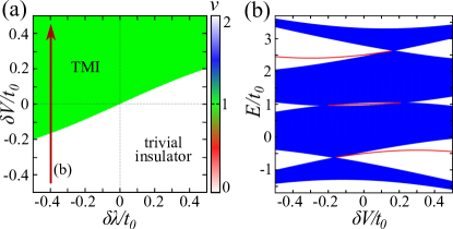
In Fig. 6(a), we show a quarter-filling $\delta V$-$\delta\lambda$ phase diagram with respect to the $\mathbb{Z}_{2}$ invariant of Eq. (2) for $\beta=\gamma=1/4$, where the corresponding unit cell comprises four lattice sites. The modulation phases are chosen such that the model respects mirror symmetry. The Rashba term preserves this symmetry if $\phi_{\lambda,m}=0$ or $\pi$, whereas the on-site term is reflection symmetric for $\phi_{V,m}=-\beta\pi$ or $(1-\beta)\pi$.Lau et al. (2015) Again, we identify two distinct topological phases. The shape of the phase boundary is mainly influenced by the relative magnitude of $\lambda_{0}$ and $V_{0}$. Moreover, the phase with nontrivial $\mathbb{Z}_{2}$ invariant features characteristic Kramers pairs at the end points of the corresponding wire. This is demonstrated in Fig. 6(b) for a path through the phase diagram at constant $\delta\lambda$ and variable $\delta V$. At quarter filling, end states are absent for small values of $\delta V$. However, if we increase $\delta V$ the bulk energy gap closes and reopens again, revealing two degenerate Kramers pairs localized at the end points of the wire. We also observe localized Kramers pairs at filling fractions $1/2$ and $3/4$ that can be attributed to a nontrivial $\mathbb{Z}_{2}$ invariant.

In addition, we calculate end charge values of $\pm 1$ for the topological phases at $1/4$, $1/2$, and $3/4$ filling depending on whether the chemical potential is tuned above or below the degenerate in-gap Kramers pairs. On the contrary, the trivial phases exhibit no end charges. This once again verifies the bulk-boundary correspondence.

Figure 6: (color online) Phase diagram and spectra of a density- and Rashba spin-orbit-modulated semiconductor nanowire with $\beta=\gamma=1/4$, $V_{0}=0.5t_{0}$, $\lambda_{0}=0.5t_{0}$, $\delta t=0$, $\phi_{V}=3\pi/4$, and $\phi_{\lambda}=\pi$: (a) Quarter-filling phase diagram. The value of the $\mathbb{Z}_{2}$ invariant $\nu$ is indicated by pixel color. The arrow shows a path through the phase diagram. (b) Energy spectra of nanowires with open boundary conditions at fixed $\delta\lambda=-0.4t_{0}$ corresponding to $\delta V$ values along the path shown in (a). States localized at the end points of the wires are highlighted in red. Note that there are end states at filling fractions $1/4$, $1/2$, and $3/4$ in certain ranges of $\delta V$.

In general, the observed end states render an effective spin-orbit coupled quantum-dot system which can potentially be implemented to realize spin-orbit qubits.Nadj-Perge et al. (2010); Li and You (2014) We point out that the use of finger gates in a realistic system is expected to produce an equal phase modulation of the Rashba SOC and onsite potential ($\phi_{V}=\phi_{\lambda}\equiv\phi$) which breaks the mirror symmetry in our tight-binding description. However, in the $\beta\rightarrow 0$ continuum limit one has $\phi_{V,m}\rightarrow\phi_{\lambda,m}$, which shows that a density- and Rashba SOC-modulated mirror-symmetric semiconductor nanowire can be realized in practice.

V Conclusions

To conclude, we have shown that one-dimensional spin-$1/2$ fermionic systems with both time-reversal and mirror symmetry can have nontrivial topology. In particular, we have found that the partial polarization in these systems can only assume the values $0$ or $1/2$. The partial polarization can therefore be used as a topological $\mathbb{Z}_{2}$ invariant. If this number is nonzero, the system is a topological mirror insulator whose hallmark is an odd number of electronic end charges. Furthermore, these end charges are robust against weak disorder as long as the protecting mirror symmetry is preserved on average. We have checked these findings against a class of models, corresponding to generalized AAH models with SOC that realize topologically nontrivial $\mathbb{Z}_{2}$ phases. These models can be realized in Fermi gases loaded in periodical optical lattices, as well as in semiconductor nanowires with perpendicular modulated voltage gates. In the latter setup the characteristic pairs of in-gap end states realize an effective spin-orbit coupled double-quantum-dot system potentially relevant for spin-orbit qubits.

We thank Guido van Miert for stimulating discussions, and acknowledge the financial support of the Future and Emerging Technologies (FET) programme within the Seventh Framework Programme for Research of the European Commission under FET-Open grant number: 618083 (CNTQC). This work has been supported by the Deutsche Forschungsgemeinschaft under Grant No. OR 404/1-1 and SFB 1143. JvdB acknowledges support from the Harvard-MIT Center for Ultracold Atoms.

Appendix A Quantized partial polarization

In the following, we briefly review the concept of partial polarization and show that its value is quantized in the presence of reflection symmetry.

Let us start with the general charge polarization $P_{\rho}$. It is a measure for the electric dipole moment per unit cell and can be elegantly written in terms of the Berry connectionZak (1989); King-Smith and Vanderbilt (1993); Resta (1994, 2000):

$$P_{\rho}=\frac{1}{2\pi}\int_{-\pi/a}^{\pi/a}dk\>\mathcal{A}(k),$$ (6)

with the $U(1)$ Berry’s connection

$$\mathcal{A}(k)=i\sum_{n}\langle u_{k,n}|\partial_{k}|u_{k,n}\rangle.$$ (7)

Here, $|u_{k,n}\rangle$ is the lattice-periodic part of a Bloch state at momentum $k$ and band index $n$, $a$ is the lattice constant, $q=-e$ is the electron charge, and the sum is over all occupied bands. Since the right-hand side of Eq. (6) is equivalent to the famous Berry phase Zak (1989) times a factor, $P_{\rho}$ is in general only defined up to an integer and can assume any value in between.

In the context of time-reversal invariant topological insulators, Fu and Kane introduced the notion of partial polarization Fu and Kane (2006). For this, they made use of the well-known Kramers’ theorem: for a time-reversal symmetric system with half-integer total spin, every energy level is evenly degenerate. For a translationally invariant system this is equivalent to saying that every Bloch state at $k$ comes with a time-reversed degenerate partner at $-k$. In particular, states at the time-reversal invariant momenta $k=0$ and $\pi/a$ must be evenly degenerate. Hence, a fully gapped system must have an even number of occupied energy bands. Assuming, for simplicity, there are no other degeneracies than those required by time-reversal symmetry, we can divide the $2N$ occupied bands into $N$ pairs subject to Fu and Kane (2006)

$$|u_{-k,\alpha}^{\mathrm{I}}\rangle=-e^{i\chi_{\alpha}(k)}\,\Theta|u_{k,\alpha}^{\mathrm{II}}\rangle,$$ (8)

where $\Theta$ is the antiunitary time-reversal operator with $\Theta^{2}=-1$, $\alpha=1,\ldots,N$, and I, II are the two time-reversed channels. Then, the partial polarizations are simply the polarizations associated with the two channels, i.e.,

$$P^{s}=\frac{1}{2\pi}\int_{-\pi/a}^{\pi/a}dk\>\mathcal{A}^{s}(k),\>\>s=\mathrm{I,II},$$ (9)

where $\mathcal{A}^{s}(k)=i\sum_{\alpha}\langle u_{k,\alpha}^{s}|\partial_{k}|u_{k,\alpha}^{s}\rangle$. It is sufficient to consider $P^{\mathrm{I}}$ only, because

$$P^{\mathrm{I}}\!-\!P^{\mathrm{II}} = \frac{1}{2\pi}\int_{-\pi/a}^{\pi/a}dk\>[\mathcal{A}^{\mathrm{I}}(k)-\mathcal{A}^{\mathrm{II}}(k)]$$ (10)

$$= \frac{1}{2\pi}\int_{0}^{\pi/a}\!\!dk\>[\mathcal{A}^{\mathrm{I}}(k)\!+\!\mathcal{A}^{\mathrm{I}}(-k)\!-\!\mathcal{A}^{\mathrm{II}}(k)\!-\!\mathcal{A}^{\mathrm{II}}(-k)]$$

$$= \frac{1}{2\pi}\sum_{\alpha}\int_{0}^{\pi/a}dk\>[\partial_{k}\chi_{\alpha}(k)-\partial_{k}\chi_{\alpha}(-k)]$$

$$= \frac{1}{2\pi}\underbrace{\sum_{\alpha}[\chi_{\alpha}(\pi/a)-\chi_{\alpha}(-\pi/a)]}_{=2\pi m,\>m\in\mathbb{Z}}=m\in\mathbb{Z},$$

where we have used that

$$\mathcal{A}^{\mathrm{I}}(-k) = i\sum_{\alpha}\langle u_{-k,\alpha}^{\mathrm{I}}|\partial_{-k}|u_{-k,\alpha}^{\mathrm{I}}\rangle$$ (11)

$$= -i\sum_{\alpha}e^{-i\chi_{\alpha}(k)}\langle\Theta u_{k,\alpha}^{\mathrm{II}}|\partial_{k}|e^{i\chi_{\alpha}(k)}\Theta u_{k,\alpha}^{\mathrm{II}}\rangle$$

$$= -i\sum_{\alpha}\langle\Theta u_{k,\alpha}^{\mathrm{II}}|\partial_{k}\Theta u_{k,\alpha}^{\mathrm{II}}\rangle+\sum_{\alpha}\partial_{k}\chi_{\alpha}(k)$$

$$= -i\sum_{\alpha}\langle\Theta^{2}\partial_{k}u_{k,\alpha}^{\mathrm{II}}|\Theta^{2}u_{k,\alpha}^{\mathrm{II}}\rangle+\sum_{\alpha}\partial_{k}\chi_{\alpha}(k)$$

$$= -i\sum_{\alpha}\langle\partial_{k}u_{k,\alpha}^{\mathrm{II}}|u_{k,\alpha}^{\mathrm{II}}\rangle+\sum_{\alpha}\partial_{k}\chi_{\alpha}(k)$$

$$= \mathcal{A}^{\mathrm{II}}(k)+\sum_{\alpha}\partial_{k}\chi_{\alpha}(k),$$

with the properties $\langle\Theta v|\Theta w\rangle=\langle w|v\rangle$ and $\Theta^{2}=-1$ of the antiunitary time-reversal operator. Hence, we have $P^{\mathrm{II}}=P^{\mathrm{I}}\,\mathrm{mod}\,1$.

On the other side, if the system preserves mirror symmetry with

$$\mathcal{M}\mathcal{H}(k)\mathcal{M}^{-1}=\mathcal{H}(-k)\>\textrm{ and }\>[\mathcal{M},\Theta]=0,$$ (12)

where $\mathcal{H}(k)$ is the Bloch Hamiltonian of the system and $\mathcal{M}$ is the reflection operator, we further have $P_{\mathrm{I}}=-P_{\mathrm{I}}\,\mathrm{mod}\,1$. This can be seen as follows: assume again for simplicity that we have no other degeneracies than those required by time-reversal symmetry. Then, we can write, similar to Eq. (8),

$$|\tilde{u}^{\mathrm{I}}_{\alpha}(-k)\rangle:=-e^{i\beta(k)}\mathcal{M}|u^{\mathrm{II}}_{\alpha}(k)\rangle,$$ (13)

where $|\tilde{u}^{\mathrm{I}}_{\alpha}(k)\rangle$ is an eigenstate of the Hamiltonian. Moreover, we can always choose $|u^{\mathrm{II}}_{\alpha}(k)\rangle$ such that $|\tilde{u}^{\mathrm{I}}_{\alpha}(k)\rangle$ is equal to $|u^{\mathrm{I}}_{\alpha}(k)\rangle$ up to a phase,

$$|\tilde{u}^{\mathrm{I}}_{\alpha}(k)\rangle=e^{i\lambda(k)}|u^{\mathrm{I}}_{\alpha}(k)\rangle.$$ (14)

Then, using Eqs. (8), (13) and $[\mathcal{M},\Theta]=0$, we easily see that

$$|u^{\mathrm{I}}_{\alpha}(k)\rangle=-e^{i[\chi(-k)+\beta(-k)]}\mathcal{M}\Theta|\tilde{u}^{\mathrm{I}}_{\alpha}(k)\rangle$$ (15)

With this, we get

$$P^{\mathrm{I}} = \frac{i}{2\pi}\sum_{\alpha}\int_{-\pi/a}^{\pi/a}dk\>\langle u_{k,\alpha}^{\mathrm{I}}|\partial_{k}|u_{k,\alpha}^{\mathrm{I}}\rangle$$ (16)

$$\overset{\eqref{eq:utilde_u_relation_2}}{=} \frac{i}{2\pi}\sum_{\alpha}\int_{-\pi/a}^{\pi/a}dk\>\langle\mathcal{M}\Theta\tilde{u}_{k,\alpha}^{\mathrm{I}}|\partial_{k}\mathcal{M}\Theta|\tilde{u}_{k,\alpha}^{\mathrm{I}}\rangle$$

$$-\frac{1}{2\pi}\underbrace{\sum_{\alpha}\int_{-\pi/a}^{\pi/a}\!\!\!dk\>\partial_{k}[\chi(-k)\!+\!\beta(-k)]}_{=2\pi n,\>n\in\mathbb{Z}}.$$

Since $P^{\mathrm{I}}$ is defined only up to an integer, we drop the second term and continue as follows

$$P^{\mathrm{I}} = \frac{i}{2\pi}\sum_{\alpha}\int_{-\pi/a}^{\pi/a}dk\>\langle(\mathcal{M}\Theta)^{\dagger}\partial_{k}\mathcal{M}\Theta\tilde{u}_{k,\alpha}^{\mathrm{I}}|\tilde{u}_{k,\alpha}^{\mathrm{I}}\rangle$$ (17)

$$= -\frac{i}{2\pi}\sum_{\alpha}\int_{-\pi/a}^{\pi/a}dk\>\langle\tilde{u}_{k,\alpha}^{\mathrm{I}}|\partial_{k}|\tilde{u}_{k,\alpha}^{\mathrm{I}}\rangle$$

$$\overset{\eqref{eq:utilde_u_relation_1}}{=} -\frac{i}{2\pi}\sum_{\alpha}\int_{-\pi/a}^{\pi/a}dk\>\langle u_{k,\alpha}^{\mathrm{I}}|e^{-i\lambda(k)}\partial_{k}e^{i\lambda(k)}|u_{k,\alpha}^{\mathrm{I}}\rangle$$

$$= -P^{\mathrm{I}}+m,\>m\in\mathbb{Z},$$

where we have used that $\mathcal{M}\Theta$ is antiunitary with properties $\langle(\mathcal{M}\Theta)^{\dagger}v|w\rangle=\langle\mathcal{M}\Theta w|v\rangle$ and $(\mathcal{M}\Theta)^{\dagger}\mathcal{M}\Theta=1$.

In conclusion, we have shown that $P^{\mathrm{I}}=-P^{\mathrm{I}}\,\mathrm{mod}\,1$. This means that $P^{I}$ can only assume the values $0$ or $1/2$ modulo $1$ and is therefore quantized.

Appendix B Smooth $U(N)$ gauge for 1D systems

The topological invariant defined in Eq. (2) requires a continuous gauge. In the following, we are going to present a method to construct such a gauge from numerically obtained eigenstates of a 1D system. The discussion closely follows the appendix of Ref. Soluyanov and Vanderbilt, 2012.

Let us consider an isolated set of $N$ bands, i.e., the bands can cross each other but shall have no crossings with other bands outside the considered set. Furthermore, consider a discrete uniform $k$ mesh of $M+1$ points $\{k_{j}\}$, $j\in[1,M+1]$, where $k_{j+1}=k_{j}+\Delta$ and $k_{M+1}=k_{1}+G$ with a reciprocal lattice vector $G$. We label the corresponding eigenstates along the mesh $|\tilde{u}_{nk_{j}}\rangle$, where $n$ is the band index. If these states are obtained from a numerical diagonalization routine, they will in general have random phases. It is easy to see that in the limit $M\rightarrow\infty$ such a choice of phases is highly non-differentiable.

In order to construct a smooth numerical gauge, we have to define what we mean by “smooth” for a discrete mesh. This can be done by requiring that the states remain as parallel as possible as we move along a path from $k_{1}$ to $k_{N+1}$. In other words, the change in the states should be orthogonal to the states themselves. The corresponding gauge is called parallel transport gauge. For a single isolated band this can be realized by choosing the phases of the Bloch states such that the overlap $\langle u_{nk_{j}}|u_{nk_{j+1}}\rangle$ is real and positive. For $N$ bands, one has to require that the overlap matrix $L_{mn}=\langle u_{mk_{j}}|u_{nk_{j+1}}\rangle$ is hermitian with only positive eigenvalues.

We are now going to explain how a parallel-transport gauge can be constructed in practice. We start from the initial point $j=1$ where we set $|u_{nk_{1}}^{\prime}\rangle=|\tilde{u}_{nk_{1}}\rangle$. Then, at each subsequent $k_{j+1}$ we have to rotate the states $|\tilde{u}_{nk_{j+1}}\rangle$ by a unitary matrix $U$ in such a way that the overlap matrix $\tilde{L}$ becomes hermitian and positive. This is accomplished by employing a singular value decomposition. More specifically, $\tilde{L}$ can be written as $\tilde{L}=V\Sigma W^{\dagger}$, where $V$ and $W$ are unitary and $\Sigma$ is positive real diagonal. If we now set $U=WV^{\dagger}$ and transform the states as

$$|u_{nk_{j+1}}^{\prime}\rangle=\sum_{m}^{N}U_{mn}(k_{j+1})|\tilde{u}_{mk_{j+1}}\rangle,$$ (18)

the new overlap matrix becomes $L^{\prime}=V\Sigma V^{\dagger}$, which is hermitian and positive. Repeating this for the entire $k$ mesh, we finally get a set of states $|u_{nk_{j}}^{\prime}\rangle$ that are smooth in the sense specified above. However, states at $k_{1}$ and $k_{N+1}$ will in general differ by a unitary transformation $\Lambda$ and are, thus, not mapped onto themselves via parallel transport. The matrix $\Lambda$ corresponds to a non-Abelian analog of the Berry phase and has eigenvalues of the form $\lambda_{l}=e^{i\phi_{l}}$.

The periodicity can be restored in the following way: we first determine the unitary matrix $S$ that diagonalizes $\Lambda$. We then rotate all states at all $k_{j}$ by $S$. This results in a gauge in which the new states correspond to a diagonal $\Lambda$ with eigenvalues $e^{i\phi_{l}}$. Finally, we spread the residual phase differences over the $k$ mesh,

$$|u_{lk_{j}}\rangle=e^{i(j-1)\phi_{l}/M}|u_{lk_{j}}^{\prime}\rangle.$$ (19)

Eventually, we have constructed a smooth, periodic gauge for the set of $N$ bands. Note, however, that the new states $|u_{lk_{j}}\rangle$ are in general not eigenstates of the Hamiltonian. Nevertheless, at each $k_{j}$ they span the eigenspace corresponding to the $N$ bands. They can therefore be used for the calculation of $U(N)$-invariant quantities like the partial polarization.

References

- Klitzing et al. (1980) K. v. Klitzing, G. Dorda, and M. Pepper, Phys. Rev. Lett. 45, 494 (1980).
- Thouless et al. (1982) D. J. Thouless, M. Kohmoto, M. P. Nightingale, and M. den Nijs, Phys. Rev. Lett. 49, 405 (1982).
- Kohmoto (1985) M. Kohmoto, Ann. Phys. 160, 343 (1985).
- Bernevig et al. (2006) B. A. Bernevig, T. L. Hughes, and S.-C. Zhang, Science 314, 1757 (2006).
- König et al. (2007) M. König, S. Wiedmann, C. Brüne, A. Roth, H. Buhmann, L. W. Molenkamp, X.-L. Qi, and S.-C. Zhang, Science 318, 766 (2007).
- Xia et al. (2009) Y. Xia, D. Qian, D. Hsieh, L. Wray, A. Pal, H. Lin, A. Bansil, D. Grauer, Y. S. Hor, R. J. Cava, and M. Z. Hasan, Nat Phys 5, 398 (2009).
- Rasche et al. (2013) B. Rasche, A. Isaeva, M. Ruck, S. Borisenko, V. Zabolotnyy, B. Büchner, K. Koepernik, C. Ortix, M. Richter, and J. van den Brink, Nat. Mater. 12, 422 (2013).
- Pauly et al. (2015) C. Pauly, B. Rasche, K. Koepernik, M. Liebmann, M. Pratzer, M. Richter, J. Kellner, M. Eschbach, B. Kaufmann, L. Plucinski, C. M. Schneider, M. Ruck, J. van den Brink, and M. Morgenstern, Nat. Phys. 11, 338 (2015).
- Kane and Mele (2005) C. L. Kane and E. J. Mele, Phys. Rev. Lett. 95, 226801 (2005).
- Liu et al. (2011) C.-C. Liu, W. Feng, and Y. Yao, Phys. Rev. Lett. 107, 076802 (2011).
- Lau and Timm (2013) A. Lau and C. Timm, Phys. Rev. B 88, 165402 (2013).
- Young et al. (2012) S. M. Young, S. Zaheer, J. C. Y. Teo, C. L. Kane, E. J. Mele, and A. M. Rappe, Phys. Rev. Lett. 108, 140405 (2012).
- Liu et al. (2014) Z. K. Liu, B. Zhou, Y. Zhang, Z. J. Wang, H. M. Weng, D. Prabhakaran, S.-K. Mo, Z. X. Shen, Z. Fang, X. Dai, Z. Hussain, and Y. L. Chen, Science 343, 864 (2014).
- Wan et al. (2011) X. Wan, A. M. Turner, A. Vishwanath, and S. Y. Savrasov, Phys. Rev. B 83, 205101 (2011).
- Huang et al. (2015) S.-M. Huang, S.-Y. Xu, I. Belopolski, C.-C. Lee, G. Chang, B. Wang, N. Alidoust, G. Bian, M. Neupane, C. Zhang, S. Jia, A. Bansil, H. Lin, and M. Z. Hasan, Nat. Commun. 6, 7373 (2015).
- Moore (2010) J. E. Moore, Nature 464, 194 (2010).
- Hasan and Kane (2010) M. Z. Hasan and C. L. Kane, Rev. Mod. Phys. 82, 3045 (2010).
- Qi and Zhang (2011) X.-L. Qi and S.-C. Zhang, Rev. Mod. Phys. 83, 1057 (2011).
- Fu (2011) L. Fu, Phys. Rev. Lett. 106, 106802 (2011).
- Ryu et al. (2010) S. Ryu, A. P. Schnyder, A. Furusaki, and A. W. W. Ludwig, New Journal of Physics 12, 065010 (2010).
- Chiu et al. (2013) C.-K. Chiu, H. Yao, and S. Ryu, Phys. Rev. B 88, 075142 (2013).
- Shiozaki and Sato (2014) K. Shiozaki and M. Sato, Phys. Rev. B 90, 165114 (2014).
- Hughes et al. (2011) T. L. Hughes, E. Prodan, and B. A. Bernevig, Phys. Rev. B 83, 245132 (2011).
- Lau et al. (2015) A. Lau, C. Ortix, and J. van den Brink, Phys. Rev. Lett. 115, 216805 (2015).
- Zhang et al. (2013) F. Zhang, C. L. Kane, and E. J. Mele, Phys. Rev. Lett. 111, 056403 (2013).
- Ueno et al. (2013) Y. Ueno, A. Yamakage, Y. Tanaka, and M. Sato, Phys. Rev. Lett. 111, 087002 (2013).
- Slager et al. (2012) R.-J. Slager, A. Mesaros, V. Juričić, and J. Zaanen, Nat Phys 9, 98 (2012).
- Zak (1989) J. Zak, Phys. Rev. Lett. 62, 2747 (1989).
- Fu and Kane (2006) L. Fu and C. L. Kane, Phys. Rev. B 74, 195312 (2006).
- King-Smith and Vanderbilt (1993) R. D. King-Smith and D. Vanderbilt, Phys. Rev. B 47, 1651 (1993).
- van Miert et al. (2016) G. van Miert, C. Ortix, and C. Morais Smith, ArXiv e-prints (2016), arXiv:1606.03232 .
- Zirnbauer (1996) M. R. Zirnbauer, Journal of Mathematical Physics 37, 4986 (1996).
- Altland and Zirnbauer (1997) A. Altland and M. R. Zirnbauer, Phys. Rev. B 55, 1142 (1997).
- Heinzner et al. (2005) P. Heinzner, A. Huckleberry, and M. R. Zirnbauer, Commun. Math. Phys 257, 725 (2005).
- Schnyder et al. (2008) A. P. Schnyder, S. Ryu, A. Furusaki, and A. W. W. Ludwig, Phys. Rev. B 78, 195125 (2008).
- Kitaev (2009) A. Kitaev, AIP Conference Proceedings 1134, 22 (2009).
- Lu and Lee (2014) Y.-M. Lu and D.-H. Lee, ArXiv e-prints , arXiv:1403.5558 (2014).
- Harper (1955) P. G. Harper, Proceedings of the Physical Society. Section A 68, 874 (1955).
- Aubry and André (1980) S. Aubry and G. André, Ann. Isr. Phys. Soc. 3, 133 (1980).
- Ganeshan et al. (2013) S. Ganeshan, K. Sun, and S. Das Sarma, Phys. Rev. Lett. 110, 180403 (2013).
- Bloch (2005) I. Bloch, Nat Phys 1, 23 (2005).
- Aidelsburger et al. (2013) M. Aidelsburger, M. Atala, M. Lohse, J. T. Barreiro, B. Paredes, and I. Bloch, Phys. Rev. Lett. 111, 185301 (2013).
- Cheuk et al. (2012) L. W. Cheuk, A. T. Sommer, Z. Hadzibabic, T. Yefsah, W. S. Bakr, and M. W. Zwierlein, Phys. Rev. Lett. 109, 095302 (2012).
- Wang et al. (2012) P. Wang, Z.-Q. Yu, Z. Fu, J. Miao, L. Huang, S. Chai, H. Zhai, and J. Zhang, Phys. Rev. Lett. 109, 095301 (2012).
- Mancini et al. (2015) M. Mancini, G. Pagano, G. Cappellini, L. Livi, M. Rider, J. Catani, C. Sias, P. Zoller, M. Inguscio, M. Dalmonte, and L. Fallani, Science 349, 1510 (2015).
- Leder et al. (2016) M. Leder, C. Grossert, L. Sitta, M. Genske, A. Rosch, and M. Weitz, ArXiv e-prints (2016), arXiv:1604.02060 .
- Zhai (2015) H. Zhai, Reports on Progress in Physics 78, 026001 (2015).
- Liu et al. (2013) X.-J. Liu, Z.-X. Liu, and M. Cheng, Phys. Rev. Lett. 110, 076401 (2013).
- Campbell et al. (2011) D. L. Campbell, G. Juzeliūnas, and I. B. Spielman, Phys. Rev. A 84, 025602 (2011).
- Wall et al. (2016) M. L. Wall, A. P. Koller, S. Li, X. Zhang, N. R. Cooper, J. Ye, and A. M. Rey, Phys. Rev. Lett. 116 (2016).
- Hofstadter (1976) D. R. Hofstadter, Phys. Rev. B 14, 2239 (1976).
- Marra et al. (2015) P. Marra, R. Citro, and C. Ortix, Phys. Rev. B 91, 125411 (2015).
- Cocks et al. (2012) D. Cocks, P. P. Orth, S. Rachel, M. Buchhold, K. Le Hur, and W. Hofstetter, Phys. Rev. Lett. 109, 205303 (2012).
- Orth et al. (2013) P. P. Orth, D. Cocks, S. Rachel, M. Buchhold, K. L. Hur, and W. Hofstetter, Journal of Physics B: Atomic, Molecular and Optical Physics 46, 134004 (2013).
- Park et al. (2016) J.-H. Park, G. Yang, J. Klinovaja, P. Stano, and D. Loss, Phys. Rev. B 94, 075416 (2016).
- Pandey and Ortix (2016) S. Pandey and C. Ortix, Phys. Rev. B 93, 195420 (2016).
- Nadj-Perge et al. (2010) S. Nadj-Perge, S. M. Frolov, E. P. A. M. Bakkers, and L. P. Kouwenhoven, Nature 468, 1084 (2010).
- Li and You (2014) R. Li and J. Q. You, Phys. Rev. B 90, 035303 (2014).
- Resta (1994) R. Resta, Rev. Mod. Phys. 66, 899 (1994).
- Resta (2000) R. Resta, Journal of Physics: Condensed Matter 12, R107 (2000).
- Soluyanov and Vanderbilt (2012) A. A. Soluyanov and D. Vanderbilt, Phys. Rev. B 85, 115415 (2012).