One-shot calculation of temperature-dependent optical spectra
and phonon-induced band-gap renormalization

Abstract

Recently, Zacharias et al. [Phys. Rev. Lett. 115, 177401 (2015)] developed a new ab initio theory of temperature-dependent optical absorption spectra and band gaps in semiconductors and insulators. In that work the zero-point renormalization and the temperature dependence were obtained by sampling the nuclear wavefunctions using a stochastic approach. In the present work, we show that the stochastic sampling of Zacharias et al. can be replaced by fully deterministic supercell calculations based on a single optimal configuration of the atomic positions. We demonstrate that a single calculation is able to capture the temperature-dependent band gap renormalization including quantum nuclear effects in direct-gap and indirect-gap semiconductors, as well as phonon-assisted optical absorption in indirect-gap semiconductors. In order to demonstrate this methodology we calculate from first principles the temperature-dependent optical absorption spectra and the renormalization of direct and indirect band gaps in silicon, diamond, and gallium arsenide, and we obtain good agreement with experiment and with previous calculations. In this work we also establish the formal connection between the Williams-Lax theory of optical transitions and the related theories of indirect absorption by Hall, Bardeen, and Blatt, and of temperature-dependent band structures by Allen and Heine. The present methodology enables systematic ab initio calculations of optical absorption spectra at finite temperature, including both direct and indirect transitions. This feature will be useful for high-throughput calculations of optical properties at finite temperature, and for calculating temperature-dependent optical properties using high-level theories such as GW and Bethe-Salpeter approaches.

I Introduction

The electron-phonon interaction plays a central role in the optical properties of solids. For example, electron-phonon couplings lead to the temperature dependence and the quantum zero-point renormalization of the critical point energies, to temperature-dependent broadening of light absorption and emission lineshapes, and to indirect optical transitions.

Recently, it has become possible to study these effects using ab initio calculations. The phonon-induced renormalization of band gaps and band structures was investigated from first principles in Refs. Allen and Cardona, 1981; Marini, 2008; Giustino et al., 2010; Gonze et al., 2011; Cannuccia and Marini, 2011; Poncé et al., 2014a, b; Antonius et al., 2014; Monserrat and Needs, 2014; Poncé et al., 2015; Lloyd-Williams and Monserrat, 2015; Monserrat, 2016a; Nery and Allen, starting from the theory of Allen and Heine (AH).Allen and Heine (1976) The optical absorption in indirect-gap semiconductors was studied from first principles in Ref. Noffsinger et al., 2012 using the classic theory of Hall, Bardeen, and Blatt (HBB),Hall et al. (1954) and in Ref. Zacharias et al., 2015 using the theory of WilliamsWilliams (1951) and LaxLax (1952) (WL). A review of the standard formalism and the of most recent literature can be found in Ref. Giustino, .

In this manuscript we focus on the WL theory, and on how to perform accurate and efficient ab initio calculations of temperature-dependent band gaps and optical spectra in semiconductors and insulators using the WL formalism. In its original formulation the WL theory was employed to study the vibrational broadening of the photoluminescence spectra of defects in solids.Williams (1951); Lax (1952) In a recent work we showed that the same theory can successfully be employed for predicting temperature dependent optical spectra and band gaps in semiconductors, including phonon-assisted indirect absorption.Zacharias et al. (2015) The reason for this success is that a perturbative treatment of the WL theory naturally leads to the adiabatic approximations of the AH and the HBB theories. In fact, as it was shown in Ref. Zacharias et al., 2015, the AH theory of temperature-dependent band structures can alternatively be derived from the WL theory by neglecting the optical matrix elements. Similarly, the adiabatic limit of the HBB theory of indirect optical absorption can be derived from the WL theory by retaining only one-phonon processes. The relations between the WL, the HBB, and the AH theory will be analyzed in detail in Sec. V.

In the WL theory,Williams (1951); Lax (1952); Patrick and Giustino (2013, 2014); Zacharias et al. (2015) the effect of quantum nuclear motion on the optical properties is described by first calculating the optical spectrum evaluated at clamped nuclei, and then taking the expectation value of this quantity over a given nuclear wavefunction. The temperature is introduced by performing a canonical average over all possible nuclear quantum states. Formally, this approach corresponds to a ‘semiclassical’ Franck-Condon approximation, whereby the initial quantum states are described by Born-Oppenheimer products of electronic and nuclear wavefunctions, and the final quantum states are replaced by a classical continuum. This approach is related to but does not coincide with the standard adiabatic approximation. An extensive discussion of the formalism and its limit of applicability can be found in Refs. Lax, 1952; Patrick and Giustino, 2014.

The key advantages of the WL method are (i) the calculations are simple and can be performed as a post-processing step on top of any electronic structure code. (ii) The formalism is agnostic of the level of theory used to describe optical excitations at clamped nuclei; therefore the same procedure can be used with any level of theory (e.g. independent-particle approximation, random-phase approximation, GW/Bethe-Salpeter), so long as the optical process can be described by means of Fermi’s Golden Rule. (iii) The method seamlessly combines the AH theory of temperature-dependent band structure and the HBB theory, of phonon-assisted indirect optical absorption.

The two main disadvantages of the WL method are (i) the calculations require the use of supercells in order to accommodate phonon wavevectors within the first Brillouin zone. (ii) The evaluation of expectation values over the nuclear wavefunctions requires calculations for many nuclear configurations. In Refs. Patrick and Giustino, 2013; Zacharias et al., 2015 the latter issue was addressed by using a stochastic approach based on importance-sampling Monte Carlo integration. In this manuscript we further improve the configurational averaging by replacing the stochastic approach of Ref. Zacharias et al., 2015 with a fully deterministic method. In particular, we demonstrate that it is possible to choose a single configuration of the nuclei yielding at once the band structure renormalization and indirect optical absorption at a given temperature. In order to demonstrate this method we report applications to silicon, diamond and gallium arsenide. Our calculated spectra and temperature dependent band gaps compare well with previous calculations and with experiment. For completeness we also provide a detailed analysis of the relation between the WL theory, the AH theory, and the HBB theory.

The organization of the manuscript is as follows: in Sec. II we briefly outline the WL expression for the temperature-dependent dielectric function, and summarize the ‘one-shot’ procedure for evaluating this expression using a single atomic configuration. In this section we also show our main results for the optical absorption spectra of Si, C, and GaAs in order to emphasize the simplicity and effectiveness of the formalism. In Sec. III we develop the formalism which is used to select the optimal atomic configuration in the one-shot calculations of Sec. II. In particular, we prove that our optimal configuration yields exact results in the limit of infinite supercell size. In Sec. IV we extend the concepts of Sec. III by showing that it is possible to deterministically select further atomic configurations in order to control and systematically reduce the error resulting from the configurational averaging. In Sec. V we discuss the link between the WL theory of temperature-dependent optical spectra, the AH theory of temperature-dependent band structures, and the HBB theory of indirect optical absorption. In Sec. VI we present our calculations of temperature-dependent band gaps for silicon, diamond, and gallium arsenide. Section VII reports all computational details of the calculations presented in this manuscript. In Sec. VIII we summarize our key findings and indicate avenues for future work. Lengthy formal derivations and further technical details are left to Appendices A-D.

II One-shot method and main results

In this section we outline the procedure for calculating temperature-dependent optical spectra using one-shot frozen-phonon calculations. For clarity we also anticipate our main results on silicon, diamond, and gallium arsenide, leaving all computational details to Sec. VII.

In the WL theory the imaginary part of the dielectric function of a solid at the temperature $T$ is given by:Zacharias et al. (2015)

$$\epsilon_{2}(\omega;T)=Z^{-1}{\sum}_{n}\exp(-E_{n}/k_{\rm B}T)\langle\epsilon_{2}(\omega;x)\rangle_{n}.$$ (1)

In this expression, $E_{n}$ denotes the energy of a nuclear quantum state evaluated in the Born-Oppenheimer approximation, $k_{\rm B}$ is the Boltzmann constant, and $Z=\sum_{n}\exp(-E_{n}/k_{\rm B}T)$ is the canonical partition function. The function $\epsilon_{2}(\omega;x)$ is the imaginary part of the macroscopic, electronic dielectric function, evaluated at clamped nuclei. For notational simplicity we indicate the set of all atomic coordinates by $x$. In the following we denote by $N$ the total number of atomic coordinates. In Eq. (1) each expectation value $\langle\cdots\rangle_{n}$ is taken with respect to the quantum nuclear state with energy $E_{n}$, and involves a multi-dimensional integration over all atomic coordinates. A detailed derivation of Eq. (1) can be found in Sec. 9.2 of Ref. Patrick and Giustino, 2014.

In order to focus on quantum nuclear effects and temperature shifts, we here describe the dielectric function at clamped nuclei using the simplest possible approximations, namely the independent-particle approximation and the electric dipole approximation:

$$\epsilon_{2}(\omega;x)=\frac{2\pi}{m_{\rm e}N_{\rm e}}\frac{\omega_{\rm p}^{2}}{\,\omega^{2}}\sum_{cv}|p_{cv}^{x}|^{2}\delta(\varepsilon_{c}^{x}-\varepsilon_{v}^{x}-\hbar\omega).$$ (2)

In this expression $m_{\rm e}$ is the electron mass, $N_{\rm e}$ is the number of electrons in the crystal unit cell, $\omega_{\rm p}$ is the plasma frequency, and $\omega$ the photon frequency. The factor 2 is for the spin degeneracy. The sum extends to the occupied Kohn-Sham states $|v^{x}\rangle$ of energy $\varepsilon_{v}^{x}$, as well as the unoccupied states $|c^{x}\rangle$ of energy $\varepsilon_{c}^{x}$. The superscripts are to keep in mind that these states are evaluated for nuclei clamped in the configuration labelled by $x$. The matrix elements of the momentum operator along the polarization direction of the photon is indicated as $p^{x}_{cv}$. In the present case we use non-local pseudopotentials and a scissor operator, therefore the momentum matrix elements are modified following Ref. Starace, 1971, as described in Sec. VII. In all the calculations presented in this manuscript the dielectric functions are obtained by first evaluating Eqs. (1) and (2) for each Cartesian direction, and then performing the isotropic average over the photon polarizations.

In principle Eq. (1) could be evaluated using the nuclear wavefunctions obtained from the solution of the nuclear Schrödinger equation with electrons in their ground state. This choice would lead to the automatic inclusion of anharmonic effects. However, for conciseness, in the present work we restrict the discussion to the harmonic approximation.

In the harmonic approximation, every many-body nuclear quantum state can be expressed as a product of Hermite functions, and the atomic displacements can be written as linear combinations of normal coordinates. Sakurai (1994) By exploiting the property of Hermite polynomials and Mehler’s formula, Watson (1933) the summation in Eq. (1) is exactly rewritten as follows:Patrick and Giustino (2014)

$$\epsilon_{2}(\omega;T)={\prod}_{\nu}\int\!dx_{\nu}\frac{\exp(-x_{\nu}^{2}/2\sigma_{\nu,T}^{2})}{\sqrt{2\pi}\sigma_{\nu,T}}\epsilon_{2}(\omega;x).$$ (3)

Here the product runs over all the normal coordinates $x_{\nu}$. In this and all following expressions it is understood that the three translational modes with zero vibrational frequency are skipped in the sums. We indicate the vibrational frequency of the $\nu$-th normal mode by $\Omega_{\nu}$. The corresponding zero-point vibrational amplitude is given by $l_{\nu}=(\hbar/2M_{\rm p}\Omega_{\nu})^{1/2}$, where $M_{\rm p}$ is a reference mass that we take equal to the proton mass. Using these conventions, the Gaussian widths in Eq. (3) are given by:

$$\sigma^{2}_{\nu,T}=(2n_{\nu,T}+1)\,l_{\nu}^{2},$$ (4)

where $n_{\nu,T}=[\exp(\hbar\omega_{\nu}/k_{\rm B}T)\!-\!1]^{-1}$ is the Bose-Einstein occupation of the $\nu$-th mode. In the reminder of this manuscript we will concentrate on the expression for the WL dielectric function given by Eq. (3).

The configurational average appearing in Eq. (3) was evaluated in Ref. Zacharias et al., 2015 using importance-sampling Monte Carlo integration.Patrick and Giustino (2013) More specifically, the Monte Carlo estimator of the integralCaflisch (1998) was evaluated by averaging over a set of atomic configurations in a Born-von Kármán supercell. Each configuration in the set was generated according to the importance function $\exp(-x_{\nu}^{2}/2\sigma_{\nu,T}^{2})/\sqrt{2\pi}\sigma_{\nu,T}$. In Ref. Zacharias et al., 2015 it was remarked that, in the case of the optical spectrum of silicon, $<10$ random samples were sufficient in order to converge the integral in Eq. (3). Furthermore, calculations performed using a single sample were found to be of comparable accuracy to fully-converged calculations. Motivated by these observations, we decided to investigate in detail why the stochastic evaluation of Eq. (3) requires only very few samples.

In Sec. III we provide a formal proof of the fact that, in the limit of large supercell, only one atomic configuration is enough for evaluating Eq. (3). In the reminder of this section we only give the optimal configuration and outline the calculation procedure, so as to place the emphasis on our main results.

In order to calculate the optical absorption spectrum (including band gap renormalization) at finite temperature using a one-shot frozen-phonon calculation, we proceed as follows:

1. We consider a $m\!\times\!m\!\times\!m$ supercell of the primitive unit cell. We determine the interatomic force constants Giustino by means of density-functional perturbation theory calculations in the primitive unit cell, using a $m\!\times\!m\!\times\!m$ Brillouin-zone grid.Baroni et al. (2001a); Giannozzi et al. (2009)

2. By diagonalizing the dynamical matrix obtained from the matrix of force constants, we determine the vibrational eigenmodes $e_{\kappa\alpha,\nu}$ and eigenfrequencies $\Omega_{\nu}$ ($\kappa$ and $\alpha$ indicate the atom and the Cartesian direction, respectively).

3. For a given temperature $T$, we generate one distorted atomic configuration by displacing the atoms from equilibrium by an amount $\Delta\tau_{\kappa\alpha}$, with:

   $$\Delta\tau_{\kappa\alpha}=(M_{\rm p}/M_{\kappa})^{\frac{1}{2}}\,{\sum}_{\nu}\,(-1)^{\nu-1}e_{\kappa\alpha,\nu}\,\sigma_{\nu,T}.\!\!\!\!\!$$ (5)

   In this expression $M_{\kappa}$ is the mass of the $\kappa$-th nucleus, and the sum runs over all normal modes. The vibrational modes are assumed to be sorted in ascending order with respect to their frequencies. In order to enforce the same choice of gauge for each vibrational mode, the sign of each eigenvector is chosen so as to have the first non-zero element positive. The prescription given by Eq. (5) will be motivated in Sec. III.

4. We calculate the dielectric function using the atomic configuration specified by Eq. (5). The result will be the temperature-dependent dielectric function at the temperature $T$.

5. We check for convergence by repeating all previous steps using increasingly larger supercells.

In Fig. 1 we present the room-temperature optical absorption coefficients of Si, C, and GaAs calculated using the procedure just outlined (red solid lines), and we compare our results with experiment (grey discs). For completeness we also show the absorption coefficients evaluated with the atoms clamped at their equilibrium positions (blue solid line). The calculations were performed on $8\!\times\!8\!\times\!8$ supercells, using density-functional theory (DFT) in the local density approximation (LDA) and a scissor correction; all computational details are provided in Sec. VII. Our present results for Si in Fig. 1(a), obtained using a single atomic configuration, are in perfect agreement with those reported in Ref. Zacharias et al., 2015 using importance-sampling Monte Carlo integration. In Fig. 1(a) we see that the spectrum calculated with the nuclei clamped in their equilibrium positions exhibit absorption only above the direct gap, as expected. At variance with these calculations, our one-shot calculation based on the WL theory correctly captures indirect transitions. In particular, this calculation is in good agreement with experiment throughout a wide range of photon energies.Green and Keevers (1995); Phillip and Taft (1964) This agreement surprisingly extends over seven orders of magnitude of the absorption coefficient. However, we should point out that our adiabatic theory does not capture the fine structure close to the absorption onset: there the non-adiabatic HBB theory gives two different slopes for phonon absorption and emission processes.Macfarlane et al. (1958); Noffsinger et al. (2012) Near the onset for direct transitions, our calculation underestimates the experimental data. This behavior is expected since we are not including electron-hole interactions, which are known to increase the oscillator strength of the $E_{1}$ peak near 3.4 eV. Benedict et al. (1998)

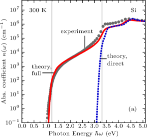
(a)

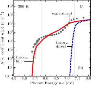
(b)

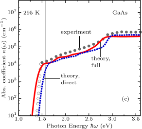
(c)

Figure 1: Absorption coefficient of (a) Si, (b) C, and (c) GaAs at room temperature. Calculations with the atoms clamped at their equilibrium positions are shown as blue dashed lines. Calculations using the WL method in the atomic configuration specified by Eq. (5) are shown as red solid lines. The experimental data for Si are from Ref. Green and Keevers, 1995 (grey discs), those for C are from Refs. Phillip and Taft, 1964 (grey discs) and Clark et al., 1964 (grey circles). Experimental data for GaAs are from Refs. Aspnes and Studna, 1983 (grey discs) and Sturge, 1962 (grey circles). The thin vertical lines indicate the direct and indirect band gaps calculated for nuclei in their equilibrium positions. The calculations were performed using $8\times 8\times 8$ supercells, using a Gaussian broadening of 30 meV for Si and C, and of 50 meV for GaAs.

In Fig. 1(b) we show our WL calculation for diamond. In this case our method correctly captures the absorption in the indirect range, however we observe more pronounced deviations between theory and experiment than in the case of Si. We assign the residual discrepancy to the inability of DFT/LDA to accurately describe the joint density of states of diamond. In fact, in contrast to the case of silicon, in diamond a simple scissor correction is not enough to mimic quasiparticle corrections.Lambert and Giustino (2013) For example, the GW corrections to the $X_{1c}$, $L_{1c}$, and $L_{3c}$ states of Si are all in the narrow range between 0.66 and 0.75 eV; instead the GW corrections to the same states of diamond span a broader range, between 1.47 and 2.04 eV.Lambert and Giustino (2013) This is expected to lead to a significant redistribution of spectral weight precisely in the range of photon energies considered in Fig. 1(b). Also in this case the strength of the $E_{1}$ peak near 7.3 eV is underestimated due to our neglecting electron-hole interactions.Benedict et al. (1998) In Fig. 1(b) we are reporting two sets of experimental data. Phillip and Taft (1964); Clark et al. (1964) These data exhibit different intensities near the absorption edge (at energies $<5.7$ eV). According to Ref Phillip and Taft, 1964, the intensity of the absorption coefficient for energies below 6.5 eV is not fully reliable. Our calculated spectrum is in closer agreement with the data from Ref Clark et al., 1964, which exhibit a sharper absorption edge. This comparison suggests that our present method might prove useful for the validation of challenging experiments, especially near the weak absorption edge. As in the case of Fig. 1(a), the fine structure features close to the absorption onset are absent in our calculation.

In Fig. 1(c) we compare the absorption coefficient calculated for GaAs with experiment. Aspnes and Studna (1983); Sturge (1962) This example clearly demonstrates that our WL calculation correctly describes the absorption spectrum of a direct-gap semiconductor. In this case the shape of the absorption coefficient is not altered, as expected, but the spectrum is redshifted as a result of the zero-point renormalization of the band structure. Also in the case of GaAs the calculated absorption coefficient underestimates the measured values. This is partially a consequence of our neglecting of excitonic effects,Rohlfing and Louie (1998) but most importantly it is a consequence of the inability of DFT/LDA to accurately describe the effective masses of GaAs. In fact, according to the standard theory of absorption in direct-gap semiconductors,Bassani and Parravicini (1975) the absorption coefficient scales as $(m^{*})^{3/4}$, where $m^{*}$ is the average isotropic effective mass. Since DFT calculations for GaAs yield masses which are up to a factor of 2 smaller than in experiment, we expect a corresponding underestimation of the absorption coefficient by up to a factor of $2^{3/4}\sim 2$. This estimate is in line with our results in Fig. 1(c). We note that this issue is not found in the case of Si [Fig. 1(a)], since the DFT/LDA effective masses of silicon are in surprising agreement with experiment.Giustino (2014) We also note that for GaAs our calculation correctly predicts phonon-assisted absorption below the direct gap. This phenomenon is related to the Urbach tail.Urbach (1953)

After discussing the comparison between our calculations and experiment, we briefly comment on the computational effort and the numerical convergence. Figure 2 shows the imaginary part of the WL dielectric function of Si, C, and GaAs evaluated at zero temperature using the procedure outlined in the previous page. In order to achieve convergence we performed calculations for supercells of increasing size, from $2\times 2\times 2$ to $8\times 8\times 8$. It is clear that large supercells are required in order to obtain converged results. Increasing the supercell size has the twofold effect of refining the sampling of the electron-phonon coupling in the equivalent Brillouin zone, and of approaching the limit where Eq. (5) becomes exact. In Fig. 2 we also report the band gaps of Si, C, and GaAs as extracted from $\epsilon_{2}(\omega)$ using the standard Tauc plots.Tauc et al. (1966) These results are in agreement with previous work and will be discussed in Sec. VI. From this figure we see that our methodology correctly describes the zero-point renormalization of the band gap of both direct- and indirect-gap semiconductors.

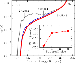
(a)

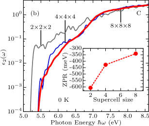
(b)

(c)

Figure 2: Convergence of the WL dielectric function as a function of supercell size: (a) Si, (b) C, and (c) GaAs. The grey curves are for calculations using $2\times 2\times 2$ supercells; blue solid lines indicate calculations using $4\times 4\times 4$ supercells; thick red solid lines are for $8\times 8\times 8$ supercells. Each curve was obtained using a single calculation, in the configuration specified by Eq. (5). For Si and C the electronic Brillouin zone was sampled using 1920, 240, and 30 k-points for the $2\times 2\times 2$, $4\times 4\times 4$, and $8\times 8\times 8$ supercells, respectively. In the case of GaAs a finer sampling was required, and we used 6400, 800 and 100 k-points, respectively. The calculations were performed using a Gaussian broadening of 30 meV for Si and C, and of 50 meV for GaAs. The insets show the band gap extracted from the Tauc plots. These values automatically include zero-point renormalization.

From Figs. 1 and 2 it should be apparent that, apart from the inherent deficiencies of the DFT/LDA approximation, with our new method it is possible to compute optical spectra and band gaps in both direct and indirect semiconductors including electron-phonon interactions, at the cost of a single supercell calculation with clamped nuclei.

In the following sections we develop the theory underlying our computational approach, and we provide an extensive set of benchmarks.

III Formal justification of Eq. (5)

In this section we provide the rationale for the choice of the optimal configuration given by Eq. (5). We start from a heuristic argument, and then we provide a formal justification.

III.1 Heuristic approach

According to Eq. (3), the WL dielectric function can be interpreted as the average of $\epsilon_{2}(\omega;x)$ over the $N$ standard normal random variables $x_{\nu}/\sigma_{\nu,T}$. Let us consider the sum of the squares of these variables, $q^{2}=\sum_{\nu}(x_{\nu}/\sigma_{\nu,T})^{2}$. The random variable $q^{2}$ follows by construction the $\chi^{2}$ distribution.Koch (1999) Owing to the central limit theorem, the $\chi^{2}$ distribution tends to a normal distribution for $N\rightarrow\infty$. More specifically, in the limit of large $N$ the variable $(q^{2}-N)/(2N)^{1/2}$ follows a standard normal distribution. As a result, as $N$ increases, the variable $q^{2}$ becomes strongly peaked at $N$, with a standard deviation $N^{1/2}$.Abramowitz and Stegun (1972) As a sanity check, we verified these limits numerically by generating one million random atomic configurations for a $4\times 4\times 4$ supercell of diamond. Based on these considerations, we infer that for large $N$ the integration in Eq. (3) is dominated by atomic configurations such that $\sum_{\nu}(x_{\nu}/\sigma_{\nu,T})^{2}=N$. This same conclusion can alternatively be reached be rewriting the integral in Eq. (3) as the product of an integral over the ‘radial’ variable $q$, and an integral over a generalized ‘angular’ variable which runs over the $(N\!-\!1)$-dimensional sphere of radius $q$.

In the absence of information about the electron-phonon coupling constants of each vibrational mode, we must assume that all modes are equally important in the evaluation of the integral in Eq. (3). Therefore the most representative sets of coordinates for evaluating the integral in Eq. (3) are those satisfying the condition $x_{\nu}/\sigma_{\nu,T}=\pm 1$ with $\nu=1,\dots N$. This is precisely what we observed in the importance-sampling Monte Carlo calculations reported in Ref. Zacharias et al., 2015. A similar conclusion was reached in Ref. Monserrat, 2016a, where the concept of ‘thermal lines’ was introduced. Here we do not follow up on the idea of thermal lines since, as we prove below, there exists one atomic configuration which yields the exact temperature-dependent dielectric function in the limit of large $N$. If we were to choose a single configuration to evaluate the integral in Eq. (3), in absence of information about the electron-phonon couplings the least-biased choice would correspond to taking random signs for each normal coordinate. This reasoning formed the heuristic basis for the choice made in Eq. (5).

III.2 Formal proof

We now proceed to demonstrate that Eq. (5) is not just a sound approximation, but it is indeed the optimal configuration for evaluating Eq. (3) using a one-shot calculation. To this aim we perform a Taylor expansion of $\epsilon_{2}(\omega;x)$ in the variables $x_{\nu}$, and then evaluate each integral $\int\!dx_{\nu}$ in Eq. (3) analytically. The result is:

$$\epsilon_{2}(\omega,T)=\epsilon_{2}(\omega)+\frac{1}{2}\sum_{\nu}\frac{\partial^{2}\epsilon_{2}(\omega;x)}{\partial x_{\nu}^{2}}\sigma_{\nu,T}^{2}+\mathcal{O}(\sigma^{4}).$$ (6)

In this expression $\epsilon_{2}(\omega)$ denotes the dielectric function evaluated for nuclei clamped in their equilibrium positions, and the term $\mathcal{O}(\sigma^{4})$ is a short-hand notation to indicate all terms of the kind $\sigma_{\nu,T}^{4}$ and higher powers.

We now consider the dielectric function calculated with the nuclei clamped in the positions specified by Eq. (5). We denote this function by $\epsilon_{2}^{1{\rm C}}(\omega;T)$, with ‘1C’ standing for ‘one configuration’. Another Taylor expansion in the normal mode coordinates yields:

$$\epsilon_{2}^{1{\rm C}}(\omega;T)=\epsilon_{2}(\omega)+\sum_{\nu}(-1)^{\nu-1}\frac{\partial\epsilon_{2}(\omega;x)}{\partial x_{\nu}}\sigma_{\nu,T}$$

$$\qquad+\frac{1}{2}\sum_{\nu\mu}(-1)^{\nu+\mu-2}\frac{\partial^{2}\epsilon_{2}(\omega;x)}{\partial x_{\nu}x_{\mu}}\sigma_{\nu,T}\sigma_{\mu,T}$$

$$\qquad+\frac{1}{6}\sum_{\nu\mu\lambda}(-1)^{\nu+\mu+\lambda-3}\frac{\partial^{3}\epsilon_{2}(\omega;x)}{\partial x_{\nu}x_{\mu}x_{\lambda}}\sigma_{\nu,T}\sigma_{\mu,T}\sigma_{\lambda,T}$$

$$\qquad+\mathcal{O}(\sigma^{4}).$$ (7)

By comparing Eqs. (6) and (III.2) we see that $\epsilon_{2}^{1{\rm C}}(\omega;T)$ and $\epsilon_{2}(\omega;T)$ do coincide up to $\mathcal{O}(\sigma^{4})$ if the following conditions hold: (i) the summations on the first and third lines of Eq. (III.2) vanish; (ii) all terms $\nu\neq\mu$ in the second line of the same equation vanish.

In general the conditions (i) and (ii) do not hold, therefore calculations of $\epsilon_{2}^{1{\rm C}}(\omega;T)$ and $\epsilon_{2}(\omega;T)$ will yield very different results. However, these conditions are fulfilled in the limit $N\rightarrow\infty$, as we show in the following. To this aim let us consider the summation on the first line of Eq. (III.2). We focus on two successive terms in the sum, $\nu$ and $\nu+1$. Assuming a vibrational density of states (vDOS) which is nonvanishing up to the highest vibrational frequency, when $N\rightarrow\infty$, then $\Omega_{\nu+1}-\Omega_{\nu}\rightarrow 0$, therefore these modes are effectively degenerate, and hence must exhibit the same electron-phonon coupling coefficients. Under these conditions we can write:

$$(-1)^{\nu-1}\frac{\partial\epsilon_{2}(\omega;x)}{\partial x_{\nu}}\sigma_{\nu,T}+(-1)^{\nu+1-1}\frac{\partial\epsilon_{2}(\omega;x)}{\partial x_{\nu+1}}\sigma_{\nu+1,T}$$

$$\qquad\simeq\frac{\partial\epsilon_{2}(\omega;x)}{\partial x_{\nu}}\sigma_{\nu,T}(-1)^{\nu-1}\left[1+(-1)\right]=0.$$ (8)

This reasoning can be repeated for every pair of vibrational modes $(\nu,\nu+1)$ appearing in the first line of Eq. (III.2). If $N$ is even, then this proves that the sum on the first line vanishes. If $N$ is odd, then there is one mode left out, but the contribution of this one mode is negligibly small for $N\rightarrow\infty$. If there are gaps in the vDOS, then the above reasoning remains valid by considering separately the frequency ranges where the vDOS is nonzero. This completes the proof that the sum in the first line of Eq. (III.2) vanishes in the limit of large $N$.

The summation in the third line of Eq. (III.2) can be analyzed along the same lines, after noticing that one can rearrange the sum as follows:

$$\sum_{\nu}\left[\frac{1}{6}\sum_{\mu\lambda}(-1)^{\mu+\lambda-3}\frac{\partial^{3}\epsilon_{2}(\omega;x)}{\partial x_{\nu}x_{\mu}x_{\lambda}}\sigma_{\nu,T}\sigma_{\mu,T}\sigma_{\lambda,T}\right](-1)^{\nu}.$$ (9)

Also in this case we can consider any pair of successive eigenmodes $\nu$ and $\nu+1$ and repeat the reasoning made above for the first line of Eq. (III.2). The result is that for $N\rightarrow\infty$ the entire sum must vanish.

If we now consider the second line of Eq. (III.2), the sum of the terms with $\nu\neq\mu$ must vanish for large $N$. In fact, the second derivatives $\partial^{2}\epsilon_{2}(\omega;x)/\partial x_{\mu}\partial x_{\nu}$ and $\partial^{2}\epsilon_{2}(\omega;x)/\partial x_{\mu}\partial x_{\nu+1}$ enter the sum with opposite signs, therefore their contribution vanishes in the limit $N$ $\rightarrow$ $\infty$. On the other hand, when $\nu=\mu$, two successive terms in the sum contribute with the same sign, yielding $2\frac{1}{2}\partial^{2}\epsilon_{2}(\omega;x)/\partial x_{\nu}^{2}$. These contributions lead precisely to the second term on the r.h.s. of Eq. (6).

Taken together, Eqs. (6)-(9) and the above discussion demonstrate that our single-configuration dielectric function, $\epsilon_{2}^{1{\rm C}}(\omega;T)$, and the exact WL dielectric function, $\epsilon_{2}(\omega;T)$, do coincide to $\mathcal{O}(\sigma^{4})$ for $N\rightarrow\infty$. It is not difficult to see that this result can be generalized to all orders in $\sigma_{\nu,T}$, therefore the following general statement holds true: in the limit of large supercell the dielectric function evaluated with the nuclei clamped in the configuration specified by Eq. (5) approaches the WL dielectric function, Eq. (3). In symbols:

$$\lim_{\vphantom{\int_{0}^{1}}N\rightarrow\infty}\,\,\epsilon_{2}^{1{\rm C}}(\omega;T)\,=\,\epsilon_{2}(\omega;T).$$ (10)

This result forms the basis for the methodology presented in this manuscript. The importance of the equivalence expressed by Eq. (10) resides in that it allows us to calculate dielectric functions at finite temperature using a single atomic configuration. This represents a significant advance over alternative techniques such as for example path-integrals molecular dynamics, importance-sampling Monte Carlo, or the direct evaluation of each term in Eq. (6) using frozen-phonon calculations for each vibrational mode.

We emphasize that, while we have proven the limit in Eq. (10), we have no information about the convergence rate of $\epsilon_{2}^{1{\rm C}}(\omega;T)$ towards the exact result $\epsilon_{2}(\omega;T)$. In principle this rate could be estimated a priori by inspecting the convergence of the Eliashberg function Allen and Cardona (1981) with the sampling of the Brillouin zone in a calculation within the primitive unit cell. In practice we found it easier to directly calculate $\epsilon_{2}^{1{\rm C}}(\omega;T)$ for supercells of increasing size. Convergence tests for Si, C, and GaAs were reported in Fig. 2. It is seen that, for these tetrahedral semiconductors, converged results are obtained for $8\times 8\times 8$ supercells. We emphasize that in Fig. 2, $\epsilon_{2}^{1{\rm C}}(\omega;T)$ is given in logarithmic scale: in a linear scale the differences between a $4\times 4\times 4$ and an $8\times 8\times 8$ calculation would be barely discernible.

Calculations using the largest supercells in Fig. 2 are obviously time-consuming. However, one should keep in mind that each line in this figure corresponds to a single calculation of the dielectric function at clamped nuclei, therefore this method enables the incorporation of temperature at low computational cost, and removes the need of configurational sampling.

In the insets of Fig. 2 we also presented the zero-point renormalization of the fundamental gaps of Si, C, and GaAs. These gaps were directly obtained from the calculated $\epsilon_{2}^{1{\rm C}}(\omega;T)$ using the standard Tauc plots.Tauc et al. (1966) Details will be discussed in Sec. VI; here we only point out that also the band gaps are calculated by using a single atomic configuration in each case. To the best of our knowledge this is the first time that calculations of temperature-dependent band gaps using a single atomic configuration have been reported.

IV Improvements using configurational averaging

There might be systems for which calculations using large supercells are prohibitively time-consuming, and the limit in Eq. (10) is practically beyond reach. For these cases it is advantageous to extend the arguments presented in Sec. III to calculations using more than one atomic configuration. In this section we show how it is indeed possible to construct a hierarchy of atomic configurations in order to systematically improve the numerical evaluation of Eq. (3) at fixed supercell size.

We restart by considering atomic configurations specified by the normal coordinates $x_{\nu}=s_{\nu}\sigma_{\nu,T}$, where the signs $s_{\nu}=+1$ or $-1$ are yet to be specified. A Taylor expansion as in Eq. (III.2) yields:

$$\epsilon_{2}^{S}(\omega;T)=\epsilon_{2}(\omega)+\sum_{\nu}s_{\nu}\frac{\partial\epsilon_{2}(\omega;x)}{\partial x_{\nu}}\sigma_{\nu,T}$$

$$\qquad+\frac{1}{2}\sum_{\nu\mu}s_{\nu}s_{\mu}\frac{\partial^{2}\epsilon_{2}(\omega;x)}{\partial x_{\nu}x_{\mu}}\sigma_{\nu,T}\sigma_{\mu,T}$$

$$\qquad+\frac{1}{6}\sum_{\nu\mu\lambda}s_{\nu}s_{\mu}s_{\lambda}\frac{\partial^{3}\epsilon_{2}(\omega;x)}{\partial x_{\nu}x_{\mu}x_{\lambda}}\sigma_{\nu,T}\sigma_{\mu,T}\sigma_{\lambda,T}$$

$$\qquad+\mathcal{O}(\sigma^{4}).$$ (11)

Here the superscript $S$ denotes the entire set of $N$ signs, $S=(s_{1},\cdots,s_{N})$. With this notation, the choice expressed by Eq. (5) corresponds to setting $S=(+\,-\,+\,-\,+\,-\,\cdots)$.

In the language of stochastic sampling, the configurations specified by $S$ and $-S$ are called an ‘antithetic pair’.Caflisch (1998) It is immediate to see that the dielectric function calculated using both $S$ and $-S$ does not contain any odd powers of $\sigma_{\nu,T}$. In fact from Eq. (IV) we have:

$$\frac{1}{2}\left[\epsilon_{2}^{S}(\omega;T)+\epsilon_{2}^{-S}(\omega;T)\right]=$$

$$\,\,\,\,\,\epsilon_{2}(\omega)+\frac{1}{2}\sum_{\nu\mu}s_{\nu}s_{\mu}\frac{\partial^{2}\epsilon_{2}(\omega;x)}{\partial x_{\nu}x_{\mu}}\sigma_{\nu,T}\sigma_{\mu,T}+\mathcal{O}(\sigma^{4}).\,\,\,\,\,\,$$ (12)

This result is already very close to the exact expansion in Eq. (6), independent of the size of the supercell.

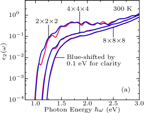
(a)

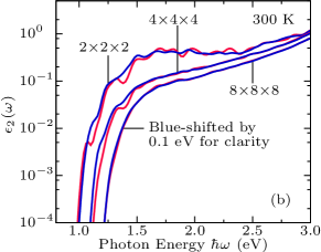
(b)

Figure 3: Effect of using multiple atomic configurations in the evaluation of the WL dielectric function of silicon. (a) Comparison between calculations performed using a single atomic configuration as specified by Eq. (5) (red solid lines), and calculations using this configuration and its antithetic pair from Eq. (IV) (blue solid line). We report calculations for increasing supercell size. (b) Comparison between calculations performed using a single configuration as in (a) (red solid lines), and those performed using 4 configurations, as specified by Eqs. (5), (IV), and (13). The curves corresponding to the $8\times 8\times 8$ supercell have been rigidly shifted by 0.1 eV: without such a shift the curves would overlap with those obtained using a $4\times 4\times 4$ supercell.

In order to obtain Eq. (6) exactly, one would need to further eliminate all terms $\nu\neq\mu$ in the sum on the second line of Eq. (IV). This elimination can be achieved systematically by considering an additional configuration $S^{\prime}$ defined as follows:

$$S\phantom{{}^{\prime}}=($$ ,

,

(13)

where for the sake of clarity we considered the case $N=8$. In practice $S^{\prime}$ is simply obtained by swapping all the signs of the second-half of the vector $S$. It is immediate to verify that the dielectric function calculated by averaging the 4 atomic configurations specified by $S$, $-S$, $S^{\prime}$, and $-S^{\prime}$ contains only half of the terms $\mu\neq\nu$ that appear in Eq. (IV). Since each individual configuration satisfies the asymptotic relation in Eq. (10), it is clear that the above calculation using 4 atomic configurations will approach the exact WL dielectric function faster as the supercell size increases.

This strategy can also be iterated by partitioning each subset in Eq. (13) in two halves, and applying a sign swap on two out of four of the resulting subsets. At each level of iteration the number of atomic configurations doubles, and the number of remaining terms $\mu\neq\nu$ in Eq. (IV) halves. For example, it is easy to verify that, by using 4, 16, and 64 configurations generated in this way, it is possible to eliminate 50%, 87.5%, and 96.875% of the terms $\mu\neq\nu$ in Eq. (IV), respectively.

In Fig. 3(a) we show the effect of using Eqs. (5) and (IV) for the calculation of the dielectric function of silicon at 300 K via 2 distinct atomic configurations. In Fig. 3(b) we repeat the calculations, this time using 4 distinct configurations, according to Eqs. (5), (IV), and (13). Here we see that increasing the number of atomic configurations suppresses spurious fluctuations in the spectra; the effect is most pronounced for the smallest supercell, which corresponds to $2\times 2\times 2$ Si unit cells. We note that, in Fig. 3, the curves corresponding to the $8\times 8\times 8$ supercell have been rigidly shifted for clarity: without such a shift the curves are almost indistinguishable from the those calculated using a $4\times 4\times 4$ supercell.

Figure 3 clearly shows that, irrespective of the configurational averaging, too small supercells may not be enough to accurately evaluate the WL dielectric function. This is easily explained by considering that, in order to correctly describe an indirect absorption onset, we need a supercell which can accommodate phonons connecting the band extrema.

V Relation between the Williams-Lax theory, the Allen-Heine theory, and the Hall-Bardeen-Blatt theory

Having described the conceptual basis of our methodology, we now establish the link between the WL dielectric function given by Eq. (3) and the standard theory of Hall, Bardeen, and Blatt of indirect optical absorption,Hall et al. (1954) as well as the theory of temperature-dependent band structures of Allen and Heine.Allen and Heine (1976) In this section we only present the main results, leaving the mathematical details to Appendices A and B.

The HBB theory describes indirect optical absorption by means of time-dependent perturbation theory, and the final expression [see Eq. (24) below] involves the momentum matrix elements evaluated for the nuclei clamped in their equilibrium positions, $p_{cv}$, and the linear electron-phonon matrix elements:

$$g_{mn\nu}=l_{\nu}\,\langle m|\frac{\partial V}{\partial x_{\nu}}|n\rangle.$$ (14)

Here $|n\rangle$ denotes a Kohn-Sham state and $\partial V/\partial x_{\nu}$ is the variation of the Kohn-Sham potential with respect to the normal mode coordinate $x_{\nu}$. In order to make these quantities explicit in Eq. (2), we expand the momentum matrix elements $p_{cv}^{x}$ to first order in the atomic displacements, and the energies $\varepsilon_{n}^{x}$ to second order in the displacements. Using Raleigh-Schrödinger perturbation theory we find:

$$p_{cv}^{x}=p_{cv}+{\sum_{\nu n}}^{\prime}\left[\frac{p_{cn}\,g_{nv\nu}}{\varepsilon_{v}-\varepsilon_{n}}+\frac{g_{cn\nu}\,p_{nv}}{\varepsilon_{c}-\varepsilon_{n}}\right]\frac{x_{\nu}}{l_{\nu}}+\mathcal{O}(x^{2}),$$ (15)

where the primed summation indicates that we skip terms such that $n=v$ or $n=c$. Similarly the expansion of the energies yields, for example:

$$\varepsilon_{c}^{x}=\varepsilon_{c} + \sum_{\nu}g_{cc\nu}\frac{x_{\nu}}{l_{\nu}}+{\sum_{\mu\nu n}}^{\prime}\left[\frac{g_{cn\mu}g_{nc\nu}}{\varepsilon_{c}-\varepsilon_{n}}+h_{c\mu\nu}\right]\frac{x_{\mu}x_{\nu}}{l_{\mu}l_{\nu}}$$ (16)

$$+ \mathcal{O}(x^{3}),$$

with $h_{c\mu\nu}$ being the ‘Debye-Waller’ electron-phonon matrix element:Allen and Heine (1976); Allen and Cardona (1981); Patrick and Giustino (2014); Giustino

$$h_{c\mu\nu}=\frac{1}{2}l_{\mu}l_{\nu}\langle c|\frac{\partial^{2}V}{\partial x_{\mu}\partial x_{\nu}}|c\rangle.$$ (17)

To make contact with the AH theory of temperature-dependent band structures and with the HBB theory of indirect absorption, we analyze separately the cases of (i) direct gaps and (ii) indirect gaps.

V.1 Direct gaps

When the gap is direct, the optical matrix elements $p_{cv}^{x}$ in Eq. (15) are dominated by the term $p_{cv}$. In fact, if we denote by $g$ the characteristic electron-phonon matrix element and by $E_{\rm g}$ the minimum gap, and we note that $x_{\nu}/l_{\nu}\sim 1$, then the terms in the square brackets are $\sim(g/E_{\rm g})p_{cv}$, and hence can be neglected next to $p_{cv}$. This approximation is implicitly used in all calculations of optical absorption spectra which do not include phonon-assisted processes. By using this approximation in Eqs. (2) and (3) we obtain:

$$\!\!\!\epsilon_{2}(\omega;T)=\frac{2\pi}{m_{\rm e}N_{\rm e}}\frac{\omega_{\rm p}^{2}}{\,\omega^{2}}\sum_{cv}|p_{cv}|^{2}$$

$$\,\,\,\times{\prod}_{\nu}\int\!dx_{\nu}\frac{\exp(-x_{\nu}^{2}/2\sigma_{\nu,T}^{2})}{\sqrt{2\pi}\sigma_{\nu,T}}\delta(\varepsilon_{cv}+\Delta\varepsilon_{cv}^{x}-\hbar\omega),\,\,\,\,\,$$ (18)

where we have defined $\varepsilon_{cv}^{x}=\varepsilon_{c}^{x}-\varepsilon_{v}^{x}$, $\varepsilon_{cv}=\varepsilon_{c}-\varepsilon_{v}$, and $\Delta\varepsilon_{cv}^{x}=\varepsilon_{cv}^{x}-\varepsilon_{cv}$. Equation (V.1) can be rewritten by exploiting the Taylor expansion of the Dirac delta distribution in powers of $\Delta\varepsilon_{cv}^{x}$. The derivation is laborious and is reported in Appendix A. The final result is:

$$\!\!\!\epsilon_{2}(\omega;T)=\frac{2\pi}{m_{\rm e}N_{\rm e}}\frac{\omega_{\rm p}^{2}}{\,\omega^{2}}\sum_{cv}|p_{cv}|^{2}$$

$$\,\,\times\frac{1}{\sqrt{2\pi}\Gamma_{cv}}\exp\left[-\frac{\left(\varepsilon_{c,T}^{\rm AH}-\varepsilon_{v,T}^{\rm AH}-\hbar\omega\right)^{2}}{2\,\Gamma_{cv}^{2}}\right]\!+\!\mathcal{O}(\sigma^{4}).\,\,$$ (19)

In this expression, $\varepsilon_{m,T}^{\rm AH}$ denotes the temperature-dependent electron energy in the Allen-Heine theory:Allen and Heine (1976)

$$\varepsilon_{m,T}^{\rm AH}=\varepsilon_{m}+\sum_{\nu}\left[{\sum_{n}}^{\prime}\frac{|g_{mn\nu}|^{2}}{\varepsilon_{m}-\varepsilon_{n}}+h_{m\nu\nu}\,\right](2n_{\nu}+1).$$ (20)

In particular, the first term in the square brackets is the Fan self-energy correction, while the second term is the Debye-Waller correction.Antončík (1955); Walter et al. (1970); Allen and Heine (1976); Allen and Cardona (1981); Cardona and Thewalt (2005) The quantity $\Gamma_{cv}$ in Eq. (V.1) is the width of the optical transition, and is defined as follows:

$$\Gamma_{cv}^{2}={\sum}_{\nu}\left|g_{cc\nu}-g_{vv\nu}\right|^{2}(2n_{\nu,T}+1).$$ (21)

Equation (V.1) shows that, in the case of direct absorption processes, the WL theory yields a dielectric function which exhibits normalized peaks at the temperature-dependent excitation energies $\varepsilon_{cv,T}^{\rm AH}$. We note that the width of the optical transitions $\Gamma_{cv}$ is similar to but does not coincide with the electron-phonon linewidth obtained in time-dependent perturbation theory, compare for example with Eq. (169) of Ref. Giustino, . This subtle difference is a direct consequence of the semiclassical approximation upon which the Williams-Lax theory is based.

To the best of our knowledge the connection derived here between the Williams-Lax theory and the Allen-Heine theory, as described by Eqs. (V.1) and (20), is a novel finding. In particular, the present analysis demonstrates that, to lowest order in perturbation theory, the WL theory of optical spectra yields the adiabatic version of the AH theory of temperature-dependent band structures.

V.2 Indirect gaps

In the case of indirect semiconductors, owing to the momentum selection rule, optical transitions near the fundamental gap are forbidden in the absence of phonons.Yu and Cardona (2010) By consequence, the optical matrix elements at equilibrium must vanish, and we can set $p_{cv}=0$ in Eq. (15). This observation represents the starting point of the classic HBB theory of indirect optical processes.Hall et al. (1954) In this case Eq. (3) becomes:

$$\epsilon_{2}(\omega;T)=\frac{2\pi}{m_{\rm e}N_{\rm e}}\frac{\omega_{\rm p}^{2}}{\,\omega^{2}}\sum_{cv}{\prod}_{\nu}\int\!dx_{\nu}\frac{\exp(-x_{\nu}^{2}/2\sigma_{\nu,T}^{2})}{\sqrt{2\pi}\sigma_{\nu,T}}$$

$$\times\left|{\sum_{\mu n}}^{\prime}\left[\frac{p_{cn}\,g_{nv\mu}}{\varepsilon_{v}-\varepsilon_{n}}+\frac{g_{cn\mu}\,p_{nv}}{\varepsilon_{c}-\varepsilon_{n}}\right]\!\frac{x_{\mu}}{l_{\mu}}\right|^{2}\delta(\varepsilon_{cv}+\Delta\varepsilon_{cv}^{x}-\hbar\omega)$$

$$+\mathcal{O}(\sigma^{4}).$$ (22)

We stress that in this expression we are only retaining those terms in Eq. (15) which are linear in the normal coordinates. This choice corresponds to considering only one-phonon processes, as it is done in the HBB theory. While multi-phonon processes are automatically included in the WL theory, in the following we do not analyze them explicitly.

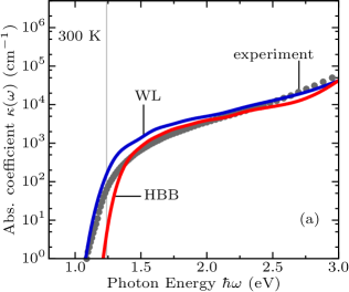
(a)

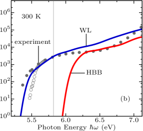
(b)

Figure 4: (a) Comparison between measured and calculated optical absorption coefficients of silicon at 300 K. The grey dots are experimental data from Ref. Green and Keevers, 1995, the red line is a calculation using the Hall-Bardeen-Blatt theory, and the blue line is a calculation using the Williams-Lax theory. (b) Comparison between measured absorption coefficient of diamond at 300 K [data from Refs. Phillip and Taft, 1964 (discs) and Clark et al., 1964 (circles)] and our calculations using the HBB theory or the WL theory. The color code is the same as in (a). In both panels the calculations were performed on $4\times 4\times 4$ supercells, using 65 random points in the electronic Brillouin zone (i.e. $>4000$ points in the Brillouin zone of the crystalline unit cell), and a Gaussian smearing of 50 meV. The thin vertical lines indicate the energy of the band gaps calculated at the equilibrium geometries.

By performing a Taylor expansion of the Dirac delta appearing in Eq. (V.2) in powers of $\Delta\varepsilon_{cv}^{x}$, as we did for the case of direct gaps, we arrive at the following expression:

$$\epsilon_{2}(\omega;T)=\frac{2\pi}{m_{\rm e}N_{\rm e}}\frac{\omega_{\rm p}^{2}}{\,\omega^{2}}\sum_{cv\nu}\left|{\sum_{n}}^{\prime}\left[\frac{p_{cn}\,g_{nv\nu}}{\varepsilon_{v}-\varepsilon_{n}}+\frac{g_{cn\nu}\,p_{nv}}{\varepsilon_{c}-\varepsilon_{n}}\right]\right|^{2}$$

$$\,\,\,\,\,\times\frac{1}{\sqrt{2\pi}\Gamma_{cv}}\exp\left[-\frac{\left(\varepsilon_{c,T}^{\rm AH}-\varepsilon_{v,T}^{\rm AH}-\hbar\omega\right)^{2}}{2\,\Gamma_{cv}^{2}}\right](2n_{\nu,T}+1)$$

$$\,\,\,\,\,+\mathcal{O}(\sigma^{6}).$$ (23)

The derivation of this result is lengthy, and is reported for completeness in Appendix B.

Equation (V.2) demonstrates that the WL theory correctly describes indirect optical absorption. In fact, if we neglect the broadening $\Gamma_{cv}$ and the temperature dependence of the band structure, we obtain the theory of Hall, Bardeen, and Blatt:Hall et al. (1954); Yu and Cardona (2010); Noffsinger et al. (2012)

$$\epsilon^{\rm HBB}_{2}(\omega;T) = \frac{2\pi}{m_{\rm e}N_{\rm e}}\frac{\omega_{\rm p}^{2}}{\,\omega^{2}}\sum_{cv\nu}\left|{\sum_{n}}^{\prime}\left[\frac{p_{cn}\,g_{nv\nu}}{\varepsilon_{v}-\varepsilon_{n}}+\frac{g_{cn\nu}\,p_{nv}}{\varepsilon_{c}-\varepsilon_{n}}\right]\right|^{2}$$ (24)

$$\times \delta\left(\varepsilon_{c}-\varepsilon_{v}-\hbar\omega\right)(2n_{\nu,T}+1).$$

The only difference between this last expression and the original HBB theory is that here the Dirac delta function does not contain the phonon energy. Physically this corresponds to stating that the WL theory provides the adiabatic limit of the HBB theory of indirect absorption.

To the best of our knowledge, this is the first derivation of the precise formal connection between the WL theory of indirect absorption, as expressed by Eq. (V.2), and the theories of Hall, Bardeen, and Blatt and of Allen and Heine, as given by Eqs. (24) and (20).

We emphasize that the adiabatic HBB theory does not incorporate the temperature dependence of the band structure, as it can be seen from Eq. (24). Instead, the WL theory includes band structure renormalization by default, see Eq. (V.2). This point is very important in view of performing predictive calculations at finite temperature.

From Eq. (V.2) we can also tell that, in order to generalize the HBB theory to include temperature-dependent band structures, one needs to incorporate the temperature dependence only in the energies corresponding to real transitions, i.e. in the Dirac deltas in Eq. (24), and not in the energies corresponding to virtual transitions, i.e. the energy denominators in the same equation.

In order to illustrate the points discussed in Secs. V.1 and V.2, we show in Fig. 4 a comparison between the absorption spectra of silicon and diamond calculated using either the HBB theory or the WL theory. For the HBB calculations we employed the adiabatic approximation and we recast Eq. (24) in the following equivalent form:

$$\epsilon^{\rm HBB}_{2}(\omega;T)=\sum_{\nu}\frac{\partial^{2}\varepsilon_{2}(\omega;x)}{\partial x_{\nu}^{2}}\sigma_{\nu,T}^{2}.$$ (25)

The equivalence between this expression and Eq. (24) is readily proven by using Eqs. (15) and (B). For the evaluation of the second derivatives for each vibrational mode we used finite-difference formulas; this operation requires $2N$ frozen-phonon calculations. In the examples shown in Fig. 4 we employed $4\times 4\times 4$ supercells, corresponding to 768 calculations on supercells containing 128 atoms. We emphasize that the WL spectrum requires instead only 1 calculation.

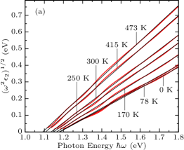
(a)

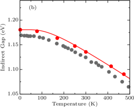
(b)

(c)

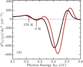
(d)

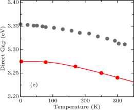
(e)

(f)

Figure 5: (a) Tauc plot for determining the indirect band gap of silicon as a function of temperature. The red lines show $(\omega^{2}\varepsilon_{2})^{1/2}$, and the thin black lines are the corresponding linear fits at each temperature. The indirect gap is obtained from the intercept with the horizontal axis. (b) Temperature-dependence of the indirect band gap of silicon: present theory (red discs) and experimental data from Ref. Alex et al., 1996 (grey discs). The solid line is a guide to the eye. The theoretical values were corrected to match the zero-point renormalization calculated as discussed in Appendix  C. (c) Convergence of the zero-point renormalization of the indirect gap of silicon with respect to the Brillouin-zone sampling of an 8$\times$8$\times$8 supercell. (d) Calculated second-derivatives of the real part of the dielectric function of silicon. (e) Temperature-dependence of the direct gap of silicon: present calculations (red discs) and experimental data from Ref. Lautenschlager et al., 1987a. The solid line is a guide to the eye. (f) Convergence of the zero-point renormalization of the direct gap of silicon with respect to the Brillouin-zone sampling. All calculations in this figure were performed using an 8$\times$8$\times$8 supercell.

Figure 4(a) compares the measured absorption coefficient of silicon (grey dots) with those calculated using the HBB theory (red line) and the WL theory (blue line). All data are for the temperature $T=300$ K. Here we see that the WL and HBB calculations yield similar spectra. However, while the optical absorption onset in the HBB theory coincides with the indirect band gap of silicon at equilibrium, the WL spectrum is red-shifted by an amount $\sim$0.1 eV, corresponding to the zero-point renormalization and the temperature shift of the gap. As a result, the WL calculation is in better agreement with experiment. We emphasize again that the agreement between theory and experiment remarkably extends over a range spanning 6 orders of magnitude, and the curves shown in Fig. 4 do not carry any empirical scaling factors.

The effect of band gap renormalization becomes more spectacular in the case of diamond, as shown in Fig. 4(b). In this case the HBB calculation misses the absorption onset by as much as $\sim$0.5 eV, while the WL theory yields an onset in agreement with experiment. The discrepancy between the prediction of the adiabatic HBB theory and experiment is understood as the result of the very large electron-phonon renormalization of the band gap of diamondGiustino et al. (2010); Cannuccia and Marini (2011); Antonius et al. (2014). In addition, the adiabatic version of the HBB theory also misses the small redshift associated with phonon-emission processes.Noffsinger et al. (2012)

We stress that the WL theory does not come without faults. The main shortcoming is that, unlike the HBB theory, it does not capture the fine structure corresponding to phonon absorption and emission processes near the absorption onset. This is a direct consequence of the semiclassical approximation underpinning the WL theory, whereby the quantization of the final vibrational states is replaced by a classical continuum.Lax (1952)

VI Band gap renormalization

VI.1 Comparison between calculations using the Williams-Lax theory and Hall-Bardeen-Blatt theory

In Sec. V we demonstrated that the imaginary part of the temperature-dependent dielectric function in the WL theory exhibits an absorption onset at the temperature-dependent band gap given by the AH theory, see Eqs. (V.1) and (V.2). This result suggests that it should be possible to extract temperature-dependent band gaps directly from calculations of $\varepsilon_{2}(\omega;T)$ or $\kappa(\omega;T)$, as it is done in experiments.

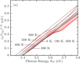
(a)

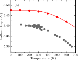
(b)

(c)

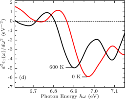
(d)

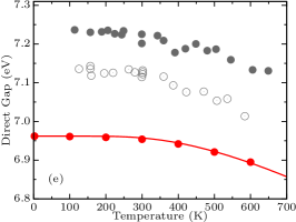
(e)

(f)

Figure 6: (a) Tauc plot to determine the indirect gap of diamond vs temperature. The red/black lines indicate $(\omega^{2}\varepsilon_{2})^{1/2}$ and the corresponding linear fits at each temperature. The indirect gap is obtained from the intercept with the horizontal axis. In this case the linear fits were performed in the range of photon energies $\hbar\omega=0$-5.6 eV. (b) Temperature-dependence of the indirect gap of diamond: this work (red discs) and experimental data from Ref. Clark et al., 1964 (grey discs). The solid line is a guide to the eye. The theoretical values were corrected to match the zero-point renormalization calculated as discussed in Appendix  C. (c) Convergence of the zero-point renormalization of the indirect gap of diamond with respect to the Brillouin-zone sampling (for an 8$\times$8$\times$8 supercell). (d) Calculated $\partial^{2}\varepsilon_{1}(\omega;T)/\partial\omega^{2}$ for diamond at two different temperatures. The $E_{0}^{\prime}$ transition is identified using the deep minimum, following Ref. Logothetidis et al., 1992. (e) Temperature-dependent direct band gap of diamond: current calculations (red discs) and experimental data from Ref. Logothetidis et al., 1992. We report the experimental data corresponding to both diamond samples II$a$ (grey circles) and II$b$ (grey discs) used in Ref. Logothetidis et al., 1992. (f) Convergence of the zero-point renormalization of the direct band gap of diamond with respect to Brillouin-zone sampling. All calculations were performed using an 8$\times$8$\times$8 supercell.

Using Eqs. (V.1) and (V.2) and the standard parabolic approximation for the band edges of three-dimensional solids,Bassani and Parravicini (1975) the following relations can be obtained after a few simple manipulations:

direct: $$\left[\omega^{2}\varepsilon_{2}(\omega;T)\right]^{2}={\rm const}\times\left(\hbar\omega-E_{{\rm g},T}\right),$$ (26)

indirect: $$\left[\omega^{2}\varepsilon_{2}(\omega;T)\right]^{\frac{1}{2}}\!={\rm const}\times\left(\hbar\omega-E_{{\rm g},T}\right).$$ (27)

Here $E_{{\rm g},T}$ is the temperature-dependent band gap, and these relations are valid near the absorption onset. Equations (26) and (27) simply reflect the joint-density of states of semiconductors, and form the basis for the standard Tauc plots which are commonly used in experiments in order to determine band gaps.Tauc et al. (1966) These relations are employed as follows: after having determined $\varepsilon_{2}(\omega;T)$, one plots $(\omega^{2}\varepsilon_{2})^{2}$ for direct-gap materials, or $(\omega^{2}\varepsilon_{2})^{1/2}$ for indirect gaps. The plot should be linear near the absorption onset, and the intercept with the horizontal axis gives the band gap $E_{{\rm g},T}$.

In the case of indirect-gap semiconductors it is not possible to use Eq. (26) in order to determine the direct band gap. Nevertheless, in these cases one can still determine the gap by analyzing second-derivative spectra of the real part of the dielectric function, $\partial^{2}\varepsilon_{1}(\omega;T)/\partial\omega^{2}$. These spectra exhibit characterisic dips, which can be used to identify the direct gap. This is precisely the procedure employed in experiments in order to measure direct band gaps.Lautenschlager et al. (1987a); Logothetidis et al. (1992); Lautenschlager et al. (1987b) In the following we use this lineshape analysis to calculate the band gaps of Si, C, and GaAs.

VI.2 Indirect semiconductors: silicon

Figure 5(a) shows the Tauc plots obtained for silicon using the WL theory. As expected from Eq. (26), we obtain straight lines over an energy range of almost 1 eV from the absorption onset. From the intercept of linear fits taken in the range 0-1.8 eV we obtain the indirect band gaps at several temperatures; the results are shown in Fig. 5(b) as red discs, and compared to experiment (grey discs). The agreement with experiment is good, with the exception of a constant offset which relates to our choice of scissor correction for the band structure of silicon (cf. Sec. VII).

In order to minimize numerical noise, we determine the zero-point renormalization of the band gap, $\Delta E_{\rm g}$, as the offset between the square root of the joint density of states calculated at equilibrium and that at $T=0$ K. This refinement is discussed in Appendix C. In this case we find $\Delta E_{\rm g}=57$ meV. Small changes of this value are expected for larger supercells and denser Brillouin-zone sampling. For completeness we show in Fig. 5(c) the convergence of the zero-point renormalization of the indirect gap with the number of ${\bf k}$-points in the supercell.

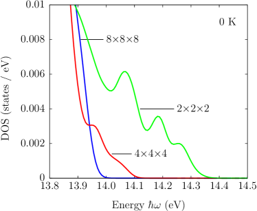
(a)

Figure 7: Density of states near the valence band edge of diamond at 0 K. Calculations were performed on $2\times 2\times 2$ (green), $4\times 4\times 4$ (red) and $8\times 8\times 8$ (blue) supercells using the one-shot WL method. We used 2560, 320 and 40 k-points, respectively, and a Gaussian broadening of 15 meV. The broken degeneracy of the valence band top, which can be seen for the $2\times 2\times 2$ supercell, tends to vanish with increasing supercell size.

Our calculated zero-point renormalization of the indirect gap of silicon is in good agreement with previous calculations and with experiment. In fact, Ref. Monserrat and Needs, 2014 reported a renormalization of 60 meV using finite-differences supercell calculations; Ref. Monserrat, 2016a reported 58 meV using Monte Carlo calculations in a supercell. Ref. Poncé et al., 2015 obtained a zero-point renormalization of 56 meV using the perturbative Allen-Heine approach. Measured values of the renormalization range between 62 and 64 meV.Cardona (2001, 2005); Cardona and Thewalt (2005)

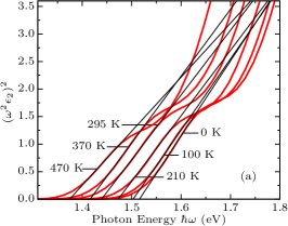
(a)

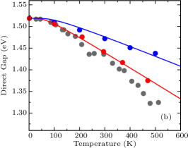
(b)

(c)

Figure 8: (a) Direct optical absorption onset in GaAs for various temperatures, as calculated using the WL theory in a 8$\times$8$\times$8 supercell. The calculations were performed in the quasi-harmonic approximation. The red curves correspond to $(\omega^{2}\varepsilon_{2})^{2}$ and the thin black lines are the corresponding linear fits (within the range of photon energies 1.42-1.62 eV). (b) Temperature-dependence of the band gap of GaAs: calculations in the quasi-harmonic approximation (red discs), calculations without considering the lattice thermal expansion (blue discs), and experimental data from Ref. Lautenschlager et al., 1987b (grey discs). The lines are guides to the eye. (c) Convergence of the calculated zero-point renormalization with respect to the number of ${\bf k}$-points, in a 8$\times$8$\times$8 supercell.

Figure 5(d) shows the second-derivative spectra, $\partial^{2}\varepsilon_{1}(\omega;T)/\partial\omega^{2}$, calculated for silicon at two temperatures. Following Ref. Lautenschlager et al., 1987a, we determine the energy of the $E_{0}^{\prime}$ transition using the first dip in the spectra. In Fig. 5(e) we compare the direct band gaps thus extracted with the experimental values. Apart from the vertical offset between our data and experiment, which relates to the choice of the scissor correction (cf. Sec. VII), the agreement with experiment is good. In order to determine the zero-point renormalization of the direct gap, we took the difference between the dips of the second-derivative spectra calculated at equilibrium and using the WL theory at $T=0$ K. We obtained a zero-point renormalization of $44$ meV, which compares well with the experimental range $25\pm 17$ meV.Lautenschlager et al. (1987a) Values in the same range were reported in previous calculations, namely 28 meV from Ref. Monserrat, 2016b and 42 meV from Ref. Poncé et al., 2015. We note that, in Ref. Monserrat, 2016b, a GW calculation on a 4$\times$4$\times$4 supercell yielded a renormalization of 53 meV. For completeness we show in Fig. 5(f) the convergence of the zero-point renormalization with respect to Brillouin-zone sampling.

VI.3 Indirect semiconductors: diamond

Figure 6(a) shows the Tauc plots calculated for diamond using the WL approach. As in the case of silicon, we determined the indirect gap as a function of temperature by means of the intercept of the linear fits with the horizontal axis; the results are shown in Fig. 6(b) together with the experimental data of Ref. Clark et al., 1964. From this comparison we see that the agreement with experiment is reasonable, however the calculations underestimate the measured renormalization. This effect has been ascribed to the fact that DFT/LDA underestimates the electron-phonon matrix elements as a consequence of the DFT band gap problem.Antonius et al. (2014) Our calculated zero-point renormalization of the indirect gap is $345$ meV. This result was obtained following the procedure in Appendix C. Our value for the zero-point renormalization is compatible with previously reported values based on DFT/LDA, namely 330 meV,Poncé et al. (2015) 334 meV,Monserrat and Needs (2014) 343 meV,Lloyd-Williams and Monserrat (2015) and 344 meV.Monserrat (2016a). Our calculations are in good agreement with the experimental values of 340 meV and 370 meV reported in Refs. Cardona, 2001, 2005. However, the use of a more recent extrapolation of the experimental data yields a renormalization of 410 meV, Monserrat et al. (2014) which is 65 meV larger than our result. Since it is known that GW quasiparticle corrections do increase the zero-point renormalization as compared to DFT/LDA,Antonius et al. (2014); Monserrat (2016b) we expect that by repeating our WL calculations in a GW framework our results will be in better agreement with the experimental data. For completeness in Fig. 6(c) we show the convergence of the zero-point renormalization with Brillouin-zone sampling (for an 8$\times$8$\times$8 supercell).

Figure 6(d) shows the second-derivative spectra of the real part of the dielectric function of diamond, as calculated from the WL theory. The direct gap of diamond was obtained in Ref. Logothetidis et al., 1992 using the deep minimum in the experimental curves; here we follow the same approach, and we report our results in Fig. 6(e). For comparison we also show the experimental data from Ref. Logothetidis et al., 1992. Apart from the vertical offset which reflects our choice of scissor correction, the calculations are in reasonable agreement with experiment. In particular we determined a zero-point renormalization of 450 meV, to be compared with the experimental ranges of $180\pm 150$ meV (sample II$a$ of Ref. Logothetidis et al., 1992) and $450\pm 370$ meV (sample II$b$ of Ref. Logothetidis et al., 1992). Our value of the zero-point renormalization is compatible with previous calculations at the DFT/LDA level, for example Ref. Lloyd-Williams and Monserrat, 2015 reported 400 meV (when using an 8$\times$8$\times$8 Supercell), Ref. Poncé et al., 2014b reported 409 meV, Ref. Monserrat, 2016b reported 410 meV (value extracted from Fig.3) and Ref. Poncé et al., 2015 reported 416 meV.

We also point out that a previous work by one of us on the electron-phonon renormalization in diamond reported a correction of 615 meV for the direct gap using DFT/LDA.Giustino et al. (2010) The origin of the overestimation obtained in Ref. Giustino et al., 2010 might be related to numerical inaccuracies when calculating electron-phonon matrix elements for unoccupied Kohn-Sham states at very high-energy, although this point is yet to be confirmed. Recent work demonstrated that GW quasiparticle corrections lead to an increase of the zero-point renormalization of the direct gap.Monserrat (2016b); Antonius et al. (2014) Calculations of optical spectra using the WL theory and the GW method are certainly desirable, but lie beyond the scope of the present work.

For completeness, in Appendix D we also investigate multi-phonon effects. In particular, we prove that WL calculations correctly yield the generalization of the adiabatic AH theory to the case of two-phonon processes, and we demonstrate that multi-phonon effects provide a negligible contribution to the band gap renormalization.

We also note incidentally that, in the case of small supercells, the band gap renormalization includes an additional spurious contribution when the band extrema are degenerate. This effect arises from a linear-order electron-phonon coupling which lifts the band degeneracy, and has already been observed in path-integral molecular dynamics calculations on diamond using a supercell with 64 atoms. Ramírez et al. (2006) This effect can easily be seen in the density of states in Fig. 7 as three separate peaks near the valence band edge. In the limit of large supercells this effect vanishes, since it arises from zone-center phonons, whose weight becomes negligibly small as $N\rightarrow\infty$.

VI.4 Direct semiconductors: gallium arsenide

Figure 8 shows our WL calculations of the temperature-dependent absorption onset and band gap of GaAs. Since GaAS is polar, we included the non-analytical part of the dynamical matrix in the calculations of the vibrational frequencies and eigenmodes.Wang et al. (2012) In this case we also took into account the thermal expansion of the lattice, which is not negligible for this semiconductor.Walter et al. (1970) To this aim we performed calculations within the quasi-harmonic approximation,Baroni et al. (2001b) that is we repeated the calculations of the normal modes for each temperature, by varying the lattice constant according to the measured thermal lattice expansion coefficient.Clec’h et al. (1989); Pierron et al. (1967)

Table 1: Vibrational zero-point renormalization of the band gaps of silicon, diamond, and gallium arsenide. Our present results based on the WL theory and Tauc plots are compared with previous DFT/LDA calculations and with experiment. The grids within the brackets indicate the sampling of the Brillouin-zone or the supercell size employed in previous calculations.

	Indirect gap			Direct gap
	Present	Previous	Experiment	Present	Previous	Experiment
Si	57	56, 58, 60	62, 64	44	28, 42	$25\pm 17$
C	345	330, 334, 343, 344	370, 410	450	409, 410, 416, 430	$180\pm 150$, $450\pm 370$
GaAs				32	23	$57\pm 29$

In Fig. 8(a) we show the direct absorption onset. In this case we extract the gap from straight-line fits of $(\omega^{2}\varepsilon_{2})^{2}$, after Eq. (26). Since the range where the function $(\omega^{2}\varepsilon_{2})^{2}$ is linear is rather narrow (due to the presence of low-lying conduction band valleys), we refine the calculation of the zero-point renormalization using the more accurate procedure discussed in Appendix C.

In Fig. 8(b) we show the calculated band gaps as a function of temperature and we compare our results to experiment. For completeness we report calculations performed without considering the thermal expansion of the lattice. Here we see that our calculations are in reasonable agreement with experiment, and that lattice thermal expansion is definitely not negligible. Using an 8$\times$8$\times$8 supercell we obtained a zero-point renormalization of 32 meV. Our value is in line with previous calculations, yielding 23 meV,Antonius et al. (2014) as well as with the experimental range of $57\pm 29$ meV. We expect that GW quasiparticle corrections will further increase the zero-point correction by $\sim$10 meV.Antonius et al. (2014) For completeness in Fig. 8(c) we show the convergence of the zero-point renormalization with the sampling of the Brillouin zone (in an 8$\times$8$\times$8 supercell).

Recently it was pointed out that, in the case of polar semiconductors, calculations based on the Allen-Heine theory exhibit a spurious divergence when the quasiparticle lifetimes are set to zero.Poncé et al. (2015); Nery and Allen The origin of this artifact relates to the Frölich electron-phonon coupling,Verdi and Giustino (2015); Sjakste et al. (2015) and has been discussed in Ref. Giustino, . In the present calculations it is practically impossible to test whether we would have a singularity in the limit of very large spercells. However, we speculate that our calculations should not diverge, since the Born-von Kármán boundary conditions effectively short-circuit the long-range electric field associated with longitudinal optical phonons. This aspect will require separate investigation.

In Table 1 we summarize all our calculations of zero-point renormalization for Si, C, and GaAs, and compare our present results with previous theory and experiment.

VII Computational setup

All calculations were performed within the local density approximation to density functional theory.Ceperley and Alder (1980); Perdew and Zunger (1981) We used norm-conserving pseudopotentials,Fuchs and Scheffler (1999) as implemented in the Quantum ESPRESSO distribution.Giannozzi et al. (2009) The Kohn-Sham wavefunctions were expanded in planewave basis sets with kinetic energy cutoffs of 40 Ry, 50 Ry, and 120 Ry for Si, GaAs and C, respectively. The interatomic force constants in the Born-von Kármán supercell were obtained as the Fourier transforms of the dynamical matrices calculated in the primitive unit cells via density functional perturbation theory.Baroni et al. (2001a)

All calculations of band gap renormalization were performed by using two atomic configurations: our optimal configuration, given by Eq. (5), and its antithetic pair, as obtained by exchanging the signs of all normal coordinates. This choice guarantees high accuracy in the lineshapes near the absorption onset. The absorption coefficients shown in Fig. 1 were calculated using $\kappa(\omega;T)=\omega\,\epsilon_{2}(\omega;T)/c\,n(\omega,T)$, where $c$ is the speed of light and $n(\omega,T)$ the refractive index calculated as $n(\omega,T)=\left[\sqrt{\epsilon_{1}^{2}(\omega;T)+\epsilon_{2}^{2}(\omega;T)}+\epsilon_{1}(\omega;T)\right]^{1/2}/\sqrt{2}$. The optical matrix elements including the commutators with the non-local components of the pseudopotential Starace (1971) were calculated using Yambo.Marini et al. (2009) In order to compensate for the DFT band gap problem, we rigidly shifted the conduction bands so as to mimic GW quasiparticle corrections. The scissor corrections were taken from previous GW calculations performed using the same computational setup for Si and C,Lambert and Giustino (2013) and from Ref. Remediakis and Kaxiras, 1999 for GaAs. In particular, we used $\Delta=0.74$ eV, 1.64 eV, and 0.53 eV for Si, C, and GaAs, respectively. The non-locality of the scissor operator was correctly taken into account in the oscillator strengths Starace (1971) via the renormalization factors $(\varepsilon_{c}-\varepsilon_{v})/(\varepsilon_{c}-\varepsilon_{v}+\Delta)$; this ensures that the $f$-sum rule is fulfilled.

The dielectric functions were calculated by replacing the Dirac deltas in Eq.(2) with Gaussians of width 30 meV for Si and C, and 50 meV, for GaAs. All calculations presented in this work were performed using 8$\times$8$\times$8 supercells of the primitive unit cell, unless specified otherwise. The sampling of the Brillouin zone of each supercell was performed using random ${\bf k}$-points, with weights determined by Voronoi triangulation.Aurenhammer (1991) In order to sample the 8$\times$8$\times$8 supercells of Si, C and GaAs we used 40, 40, and 100 random ${\bf k}$-points, respectively.

The expansion of the crystalline lattice with temperature was only considered in the case of GaAs. This choice is justified by the fact that the calculated band gaps of silicon and diamond change by less than 2 meV when using the lattice parameters at $T=0$ K and $T=300$ K. The temperature-dependence of the lattice parameters of Si and C was taken from Ref. Okada and Tokumaru, 1984; Sato et al., 2002.

VIII Conclusions and outlook

In this manuscript we developed a new ab initio computational method for calculating the temperature-dependent optical absorption spectra and band gaps of semiconductors, including quantum zero-point effects. The present work significantly expands the scope of our previous investigation in Ref. Zacharias et al., 2015, by completely removing the need for stochastic sampling of the nuclear wavefunctions. In particular we demonstrated, both using a formal proof and by means of explicit first-principles calculations, that in order to compute dielectric functions and band gaps at finite temperature it is sufficient to perform a single supercell calculation with the atoms in a well-defined configuration, as given by Eq. (5).

Using this new technique we reported the first calculations of the complete optical absorption spectra of diamond and gallium arsenide including electron-phonon interactions, and we confirmed previous results obtained for silicon in Refs. Noffsinger et al., 2012; Zacharias et al., 2015. Our calculations are in good agreement with experiment at the level of lineshape, location of the absorption onset, and magnitude of the absorption coefficient. From these calculations we extracted the temperature-dependence and the zero-point renormalization of the direct band gaps of Si, C, and GaAs, and of the indirect gaps of Si and C. Our calculations are in good agreement with previous theoretical studies.

Our present work relies on the Williams-Lax theory of optical transitions including nuclear quantum effects.Williams (1951); Lax (1952) For completeness we investigated in detail the formal relation between the WL theory, the Allen-Heine theory of temperature-dependent band structures, and the Hall-Bardeen-Blatt theory of phonon-assisted optical absorption. We demonstrated that both the AH theory and the HBB theory can be derived as low-order approximations of the WL theory.

We emphasize that our present approach enables calculations of complete optical spectra at finite temperature, including seamlessly direct and indirect optical absorption. This feature is useful in order to calculate spectra which are directly comparable to experiment in absolute terms, i.e. without arbitrarily rescaling the absorption coefficient or shifting the absorption onset to fit experiment. Our methodology will also be useful for predictive calculations of optical spectra, for example in the context of high-throughput computational screening of materials.

It is natural to think that the present approach could be upgraded with calculations of electronic structure and optical properties based on the GW/Bethe-Salpeter approach. Indeed, as it should be clear from Eq. (3), our methodology holds unchanged irrespective of the electronic structure technique employed to describe electrons at clamped nuclei. Since the present approach requires only one calculation in a large supercell, it is possible that complete GW/Bethe-Salpeter calculations of optical spectra including phonon-assisted processes will soon become feasible. In this regard we note that, recently, Ref. Lloyd-Williams and Monserrat, 2015 proposed the so-called ‘non-diagonal’ supercells in order to perform accurate supercell calculations at a dramatically reduced computational cost. In the future, it will be interesting to investigate how to take advantage of nondiagonal supercells in order to make the present methodology even more efficient.

Finally, it should be possible to generalize our present work to other important optical and transport properties. In fact, the WL theory is completely general and can be used with any property which can be described by the Fermi Golden Rule. For example, we expect that generalizations to properties such as photoluminescence or Auger recombinationKioupakis et al. (2015) should be within reach.

Appendix A Williams-Lax expression for direct absorption

In this Appendix we outline the steps leading from Eq. (V.1) to Eq. (V.1). We start by introducing the compact notation:

$$\Delta\varepsilon_{cv}^{x}=\sum_{\nu}A_{cv\nu}x_{\nu}+\sum_{\mu\nu}B_{cv\mu\nu}x_{\mu}x_{\nu}+\mathcal{O}(x^{3}),$$ (28)

where the coefficients $A_{cv\nu}$ and $B_{cv\mu\nu}$ are obtained from Eq. (16):

$$A_{cv\nu} = \frac{1}{l_{\nu}}\left(g_{cc\nu}-g_{vv\nu}\right),$$ (29)

$$B_{cv\mu\nu} = \frac{1}{l_{\mu}l_{\nu}}{\sum_{n}}^{\prime}\left[\left(\frac{g_{cn\mu}g_{nc\nu}}{\varepsilon_{c}-\varepsilon_{n}}+h_{c\mu\nu}\,\right)\right.$$ (30)

$$\left.\hskip 32.72049pt-\left(\frac{g_{vn\mu}g_{nv\nu}}{\varepsilon_{v}-\varepsilon_{n}}+h_{v\mu\nu}\right)\right].$$

Equation (V.1) can be simplified by using the Taylor expansion of the Dirac delta with respect to the energy argument. In general we have:Feller (1971)

$$\delta(\epsilon+\eta)=\sum_{n=0}^{\infty}\frac{(-1)^{n}}{n!}\left.\frac{\partial^{n}\delta}{\,\,\partial\epsilon^{n}}\right|_{\epsilon}\eta^{n},$$ (31)

therefore we can set $\varepsilon=\varepsilon_{cv}-\hbar\omega$ and $\eta=\Delta\varepsilon_{cv}^{x}$, and replace inside Eq. (V.1). We find:

$$\epsilon_{2}(\omega;T) = \frac{2\pi}{m_{\rm e}N_{\rm e}}\frac{\omega_{\rm p}^{2}}{\,\omega^{2}}\sum_{cv}|p_{cv}|^{2}\sum_{n=0}^{\infty}\frac{(-1)^{n}}{n!}\left.\frac{\partial^{n}\delta}{\partial(\hbar\omega)^{n}}\right|_{\hbar\omega-\varepsilon_{cv}}$$ (32)

$$\times {\prod}_{\nu}\int\!dx_{\nu}\frac{\exp(-x_{\nu}^{2}/2\sigma_{\nu,T}^{2})}{\sqrt{2\pi}\sigma_{\nu,T}}(\Delta\varepsilon_{cv}^{x})^{n}.$$

Now we replace $\Delta\varepsilon_{cv}^{x}$ from Eq. (28) and carry out the integrals in the coordinates $x_{\nu}$. The resulting expression does not contain the normal coordinates any more, and the various derivatives of the delta function can be regrouped using Eq. (31) in reverse. The result is:

$$\epsilon_{2}(\omega;T)=\frac{2\pi}{m_{\rm e}N_{\rm e}}\frac{\omega_{\rm p}^{2}}{\,\omega^{2}}\sum_{cv}|p_{cv}|^{2}$$

$$\times\left[\delta\!\left(\varepsilon_{cv,T}^{\rm AH}-\hbar\omega\right)+\frac{1}{2}\sum_{\nu}A_{cv\nu}^{2}\sigma_{\nu,T}^{2}\frac{\partial^{2}\delta(\hbar\omega-\varepsilon_{cv})}{\,\,\partial(\hbar\omega)^{2}}\right]$$

$$+\mathcal{O}(\sigma^{4}),$$ (33)

where $\varepsilon_{cv,T}^{\rm AH}=\varepsilon_{c,T}^{\rm AH}-\varepsilon_{v,T}^{\rm AH}$, and $\varepsilon_{m,T}^{\rm AH}$ is the temperature-dependent electron energy given by Eq. (20).

In order to make Eq. (A) more compact, it is convenient to rewrite the second term inside the square brackets by performing a Taylor expansion of the Dirac delta around $\varepsilon_{cv,T}^{\rm AH}$, and group the terms proportional to $\sigma_{\nu,T}^{4}$ and higher order inside the term $\mathcal{O}(\sigma^{4})$ at the end. This step leads to:

$$\epsilon_{2}(\omega;T)=\frac{2\pi}{m_{\rm e}N_{\rm e}}\frac{\omega_{\rm p}^{2}}{\,\omega^{2}}\sum_{cv}|p_{cv}|^{2}$$

$$\,\,\,\times\left[1+\frac{1}{2}\Gamma_{cv}^{2}\frac{\partial^{2}}{\,\,\partial(\hbar\omega)^{2}}\right]\delta\!\left(\varepsilon_{cv,T}^{\rm AH}-\hbar\omega\right)+\mathcal{O}(\sigma^{4}),$$ (34)

having defined:

$$\Gamma_{cv}^{2}={\sum}_{\nu}A_{cv\nu}^{2}\sigma_{\nu,T}^{2}={\sum_{\nu}}\left(g_{cc\nu}-g_{vv\nu}\right)^{2}(2n_{\nu,T}+1).$$ (35)

In the final step we note that the term $\partial^{2}/\partial(\hbar\omega)^{2}$ in Eq. (A) acts so as to broaden the lineshape. This is seen by using the Fourier representation of the Dirac delta, $\delta(\hbar\omega)=(2\pi\hbar)^{-1}\int dt\exp(-i\omega t)$. We find:

$$\left[1+\frac{1}{2}\Gamma_{cv}^{2}\frac{\partial^{2}}{\,\,\partial(\hbar\omega)^{2}}\right]\delta\!\left(\varepsilon_{cv,T}^{\rm AH}-\hbar\omega\right)$$

$$=\frac{1}{2\pi\hbar}\int dt\left[1-\frac{\Gamma_{cv}^{2}}{2\hbar^{2}}t^{2}\right]\exp\left(-i\frac{\varepsilon_{cv,T}^{\rm AH}-\hbar\omega}{\hbar}t\right)\!\!.\,\,$$ (36)

The term within the square brackets corresponds to the first order Taylor expansion of a Gaussian (or alternatively a Lorentzian), therefore the last expression can be rewritten as:

$$\frac{1}{2\pi\hbar}\int dt\exp\left[-\frac{\Gamma_{cv}^{2}}{2\hbar^{2}}t^{2}\right]\exp\left(-i\frac{\varepsilon_{cv,T}^{\rm AH}-\hbar\omega}{\hbar}t\right)+\mathcal{O}(\sigma^{4}),$$ (37)

where we recognize the Fourier transform of a Gaussian. An explicit evaluation of the integral yields also a Gaussian, and the final result is Eq. (V.1).

Appendix B Williams-Lax expression for indirect absorption

In this Appendix we outline the derivation of Eq. (V.2) starting from Eq. (V.2). It is convenient to introduce the notation:

$$C_{cv\mu}={\sum_{n}}^{\prime}\left[\frac{p_{cn}\,g_{nv\mu}}{\varepsilon_{v}-\varepsilon_{n}}+\frac{g_{cn\mu}\,p_{nv}}{\varepsilon_{c}-\varepsilon_{n}}\right]\!\frac{1}{l_{\mu}},$$ (38)

so that Eq. (V.2) can be written as:

$$\!\!\!\epsilon_{2}(\omega;T)=\frac{2\pi}{m_{\rm e}N_{\rm e}}\frac{\omega_{\rm p}^{2}}{\,\omega^{2}}\sum_{cv}{\prod}_{\nu}\int\!dx_{\nu}\frac{\exp(-x_{\nu}^{2}/2\sigma_{\nu,T}^{2})}{\sqrt{2\pi}\sigma_{\nu,T}}$$

$$\!\!\!\times\sum_{\mu\mu^{\prime}}C_{cv\mu}C_{cv\mu^{\prime}}x_{\mu}x_{\mu^{\prime}}\,\delta(\varepsilon_{cv}+\Delta\varepsilon_{cv}^{x}-\hbar\omega)+\mathcal{O}(\sigma^{4}).\,\,\,\,\,$$ (39)

We now write explicitly the expansion of the Dirac delta to second order in $x_{\nu}$, using Eqs. (28)-(31):

$$\delta(\varepsilon_{cv}+\Delta\varepsilon_{cv}^{x}-\hbar\omega)=\delta(\varepsilon_{cv}-\hbar\omega)$$

$$-\left.\frac{\partial\delta}{\partial(\hbar\omega)}\right|_{\hbar\omega-\varepsilon_{cv}}\left[\sum_{\nu}A_{cv\nu}x_{\nu}+\sum_{\mu\nu}B_{cv\mu\nu}x_{\mu}x_{\nu}\right]$$

$$+\frac{1}{2}\left.\frac{\partial^{2}\delta}{\partial(\hbar\omega)^{2}}\right|_{\hbar\omega-\varepsilon_{cv}}\left[\sum_{\mu\nu}A_{cv\mu}A_{cv\nu}x_{\mu}x_{\nu}\right]+\mathcal{O}(x^{3}).\,\,\,\,\,$$ (40)

By replacing the last expression in Eq. (B) and perfoming the integrations, after a few lengthy but straightforward manipulations we find:

$$\epsilon_{2}(\omega;T) = \frac{2\pi}{m_{\rm e}N_{\rm e}}\frac{\omega_{\rm p}^{2}}{\,\omega^{2}}\sum_{cv}\sum_{\nu}|C_{cv\nu}|^{2}\sigma_{\nu,T}^{2}$$ (41)

$$\times \left[1-\sum_{\mu}B_{cv\mu\mu}\sigma_{\mu,T}^{2}\frac{\partial\delta}{\partial(\hbar\omega)}\right.$$

$$+ \left.\frac{1}{2}\sum_{\mu}|A_{cv\mu}|^{2}\sigma_{\mu,T}^{2}\frac{\partial^{2}\delta}{\partial(\hbar\omega)^{2}}\right]\delta(\varepsilon_{cv}-\hbar\omega)$$

$$+ \mathcal{O}(\sigma^{6}).$$

In this expression we neglected interference terms of the type $\sum_{\mu\nu\neq\lambda\kappa}C_{cv\mu}C_{cv\lambda}B_{cv\nu\kappa}\sigma_{\nu,T}^{2}\sigma_{\kappa,T}^{2}$ next to positive-definite terms of the same order, such as for example $\sum_{\mu\nu}|C_{cv\mu}|^{2}B_{cv\nu\nu}\sigma_{\mu,T}^{2}\sigma_{\nu,T}^{2}$. This is justified since in the case of extended solids the former sum tends to zero as the phases of each term cancel out in average. In a similar spirit, we neglected terms like $2B_{cv\nu\nu}\sigma_{\nu,T}^{2}$ next to $\sum_{\mu}B_{cv\mu\mu}\sigma_{\mu,T}^{2}$. This is justified as each term in the sum is positive definite, and the number of these terms goes to infinity in extended solids.

Now Eq. (41) can be recast in the form given by Eq. (V.2) by using the Fourier representation of the Dirac delta, and following the same steps as in Appendix A, Eqs. (A)-(37). In particular, the term $\partial\delta/\partial(\hbar\omega)$ yields a shift of the excitation energies which coincides with the energy renormalization in the Allen-Heine theory, see Eq. (20). Similarly, the term $\partial^{2}\delta/\partial(\hbar\omega)^{2}$ yields a broadening of the absorption peak, which corresponds to the linewidth $\Gamma_{cv}$ of Eq. (21).

Appendix C Calculation of the zero-point band gap renormalization using the joint density of states

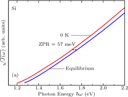
(a)

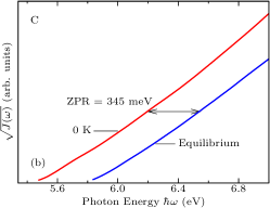
(b)

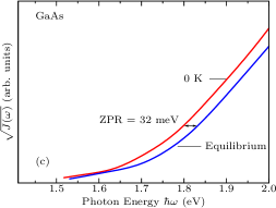
(c)

Figure C.1: Square-root of the joint density of states of (a) silicon, (b) diamond, and (c) gallium arsenide. The calculations were performed with nuclei clamped in their equilibrium positions (blue lines), and using the one-shot WL method at $T=0$ K (red lines). The horizontal offset between blue and red curves corresponds to the zero-point renormalization of the band gap in each case. The calculations for the equilibrium structures were performed in the primitive unit cells, using 20480, 20480 and 51200 random k-points for Si, C, and GaAs, respectively. The WL calculations were performed on $8\!\times\!8\!\times\!8$ supercells, using 40, 40, and 100 random k-points for Si, C, and GaAs, respectively. A Gaussian broadening of 30 meV was used in all plots.

In this Appendix we discuss an accurate procedure for determining the zero-point band gap renormalization within a supercell calculation.

We consider the joint density of states (JDOS), defined as the convolution between the density of states of valence and conduction bands:Yu and Cardona (2010)

$$J(\omega)=\sum_{cv}\delta\!\left(\varepsilon_{cv}-\hbar\omega\right).$$ (42)

Within an energy range where band extrema are parabolic, it can be shown that $J(\omega)={\rm const}\times(\hbar\omega-E_{\rm g})^{2}$. This relation holds both for direct-gap and indirect-gap semiconductors. This is the basic relation underpinning the use of Tauc’s plots in experimental spectra.Tauc et al. (1966); Bassani and Parravicini (1975) Within the WL theory, the previous relation can be shown to remain essentially unchanged:

$$J(\omega;T)=\sum_{cv}\delta\!\left(\varepsilon_{cv,T}^{\rm AH}-\hbar\omega\right)+\mathcal{O}(\sigma^{4}).$$ (43)

This result can be obtained by following the same prescription used to obtain Eq. (A). Therefore also in this case we have $J(\omega,T)={\rm const}\times(\hbar\omega-E_{{\rm g},T})^{2}$.

Using Eqs. (42) and (43) we can determine the zero-point renormalization of the band gap as the horizontal offset between the curves $J(\omega)^{1/2}$ and $J(\omega,T=0)^{1/2}$. This procedure is very accurate because we are comparing two calculations executed under identical conditions; therefore the numerical errors arising from the choice of the energy range, the Gaussian broadening and the Brillouin-zone sampling tend to cancel out.

In Figs. C.1 (a), (b) and (c) we show the square-root of the joint density of states of silicon, diamond and gallium arsenide, calculated with the atoms at their relaxed positions (red lines), and the corresponding one-shot WL calculations at 0 K (blue lines). In all cases the two curves are parallel, and the horizontal offset between the curves gives the zero-point renormalization. Using this method, our values of the zero-point renormalization of the band gaps of Si, C and GaAs are 57 meV, 345 meV and 32 meV, respectively.

We note that this new procedure critically requires the JDOS as opposed to the optical spectra, since in the case of indirect-gap materials we have no optical absorption below the direct gap in the equilibrium structure.

Appendix D Analysis of multi-phonon contributions to the band gap renormalization of diamond

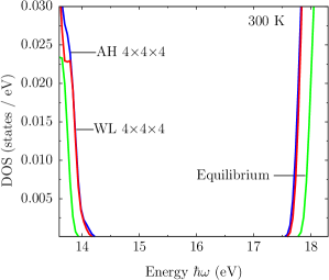
(a)

Figure D.1: Density of states of diamond close to the valence and conduction band edges: calculation at the equilibrium geometry (green line), one-shot WL calculation (red line), and AH calculation (blue line). The latter two calculations were performed for $T=300$ K, using a $4\times 4\times 4$ supercell and 65 k-points in the Brillouin zone of the supercell. The calculation with the atoms at their equilibrium geometry was carried out within the primitive unit cell, using 4160 k-points. A Gaussian smearing of 30 meV was used for all curves.

In this Appendix we first establish the link between our one-shot WL calculation and multi-phonon processes in the AH theory, and then show that multi-phonon effects are essentially negligible in diamond.

We perform an expansion of the Kohn-Sham energy $\varepsilon_{n}^{x}$ in terms of normal-mode coordinates to obtain:

$$\epsilon_{n}^{x} = \epsilon_{n}+\sum_{\nu}\frac{\partial\epsilon_{n}^{x}}{\partial x_{\nu}}x_{\nu}+\frac{1}{2}\sum_{\mu\nu}\frac{\partial^{2}\epsilon_{n}^{x}}{\partial x_{\mu}\partial x_{\nu}}x_{\mu}x_{\nu}$$ (44)

$$+ \frac{1}{3!}\sum_{\mu\nu\lambda}\frac{\partial^{3}\epsilon_{n}^{x}}{\partial x_{\mu}\partial x_{\nu}\partial x_{\lambda}}x_{\mu}x_{\nu}x_{\lambda}$$

$$+ \frac{1}{4!}\sum_{\mu\nu\lambda\kappa}\frac{\partial^{4}\epsilon_{n}^{x}}{\partial x_{\mu}\partial x_{\nu}\partial x_{\lambda}\partial x_{\kappa}}x_{\mu}x_{\nu}x_{\lambda}x_{\kappa}+\mathcal{O}(x^{5}).$$

The AH theory is obtained by taking the thermal averages of $x_{\nu}$, $x_{\mu}x_{\nu}$, $x_{\mu}x_{\nu}x_{\lambda}$, and $x_{\mu}x_{\nu}x_{\lambda}x_{\kappa}$. The result is:

$$\epsilon_{n,T}^{\rm AH} = \epsilon_{n}+\frac{1}{2}\sum_{\nu}\frac{\partial^{2}\epsilon_{n}^{x}}{\partial x_{\nu}^{2}}\sigma_{\nu,T}^{2}+\frac{3}{4!}\sum_{\mu\neq\nu}\frac{\partial^{4}\epsilon_{n}^{x}}{\partial x_{\mu}^{2}\partial x_{\nu}^{2}}\sigma_{\mu,T}^{2}\sigma_{\nu,T}^{2}$$ (45)

$$+ \frac{3}{4!}\sum_{\nu}\frac{\partial^{4}\epsilon_{n}^{x}}{\partial x_{\nu}^{4}}\sigma_{\nu,T}^{4}+\mathcal{O}(\sigma^{6}).$$

The second term on the r.h.s. represents the energy-level renormalization within the AH theory, and accounts only for single-phonon processes. This was discussed in Sec. V. The third and fourth terms of the r.h.s. represent the two-phonon contribution to the energy-level renormalization in the AH theory.

Now we show how our one-shot calculation correctly captures the two-phonon contribution. By replacing our ‘optimal configuration’ from Sec. II inside Eq. (44), and taking the limit of $N\rightarrow\infty$, we find:

$$\epsilon_{n,T}^{\rm 1C} = \epsilon_{n}+\frac{1}{2}\sum_{\nu}\frac{\partial^{2}\epsilon_{n}^{x}}{\partial x_{\nu}^{2}}\sigma_{\nu,T}^{2}+\frac{3}{4!}\sum_{\mu\neq\nu}\frac{\partial^{4}\epsilon_{n}^{x}}{\partial x_{\mu}^{2}\partial x_{\nu}^{2}}\sigma_{\mu,T}^{2}\sigma_{\nu,T}^{2}$$ (46)

$$+ \frac{1}{4!}\sum_{\nu}\frac{\partial^{4}\epsilon_{n}^{x}}{\partial x_{\nu}^{4}}\sigma_{\nu,T}^{4}+\mathcal{O}(\sigma^{6}).$$

By comparing Eqs. (45) and (46) we see that the one-shot method and the fourth-order AH theory give the same result, except for a contribution $\frac{2}{4!}\sum_{\nu}\frac{\partial^{4}\epsilon_{n}^{x}}{\partial x_{\nu}^{4}}\sigma_{\nu,T}^{4}$. In the limit of $N\rightarrow\infty$ this contribution is negligible as compared to the other terms. This reasoning is analogous to the discussion in Appendix B.

Therefore we can conclude that the one-shot WL method captures not only the standard one-phonon processes of the AH theory, but also multi-phonon contributions. The two-phonon contributions are identical to what one would obtain from carrying the AH theory to fourth-order in the atomic displacements.

In order to investigate the energy-level renormalization coming from two-phonon and higher multi-phonon processes, we calculated the density of states (DOS) of diamond within (i) the standard (one-phonon) AH theory, and (ii) the one-shot WL method. These quantities are shown in Fig. D.1, for $T=300$ K, in blue and red, respectively. For comparison, we also show the DOS calculated with the atoms in their equilibrium positions (green). The AH correction to the DOS was obtained by evaluating the derivatives $\partial^{2}\epsilon_{n}^{x}/\partial x_{\nu}^{2}$ by means of finite differences. This required 2N frozen-phonon calculations.

Figure D.1 shows that the DOS obtained from the standard AH theory and from the one-shot WL method (which includes multi-phonon effects) essentially coincide. This demonstrates that multi-phonon contributions to the band gap renormalization are negligible in diamond.

References

- Allen and Cardona (1981) P. B. Allen and M. Cardona, Phys. Rev. B 23, 1495 (1981).
- Marini (2008) A. Marini, Phys. Rev. Lett. 101, 106405 (2008).
- Giustino et al. (2010) F. Giustino, S. G. Louie, and M. L. Cohen, Phys. Rev. Lett. 105, 265501 (2010).
- Gonze et al. (2011) X. Gonze, P. Boulanger, and M. Côté, Ann. Phys. 523, 168 (2011).
- Cannuccia and Marini (2011) E. Cannuccia and A. Marini, Phys. Rev. Lett. 107, 255501 (2011).
- Poncé et al. (2014a) S. Poncé, G. Antonius, Y. Gillet, P. Boulanger, J. Laflamme Janssen, A. Marini, M. Côté, and X. Gonze, Phys. Rev. B 90, 214304 (2014a).
- Poncé et al. (2014b) S. Poncé, G. Antonius, P. Boulanger, E. Cannuccia, A. Marini, M. Côté, and X. Gonze, Comput. Mater. Science 83, 341 (2014b).
- Antonius et al. (2014) G. Antonius, S. Poncé, P. Boulanger, M. Côté, and X. Gonze, Phys. Rev. Lett. 112, 215501 (2014).
- Monserrat and Needs (2014) B. Monserrat and R. J. Needs, Phys. Rev. B 89, 214304 (2014).
- Poncé et al. (2015) S. Poncé, Y. Gillet, J. Laflamme Janssen, A. Marini, M. Verstraete, and X. Gonze, J. Chem. Phys. 143 (2015).
- Lloyd-Williams and Monserrat (2015) J. H. Lloyd-Williams and B. Monserrat, Phys. Rev. B 92, 184301 (2015).
- Monserrat (2016a) B. Monserrat, Phys. Rev. B 93, 014302 (2016a).
- (13) J. P. Nery and P. B. Allen, arXiv:1603.04269 .
- Allen and Heine (1976) P. B. Allen and V. Heine, J. Phys. C 9, 2305 (1976).
- Noffsinger et al. (2012) J. Noffsinger, E. Kioupakis, C. G. Van de Walle, S. G. Louie, and M. L. Cohen, Phys. Rev. Lett. 108, 167402 (2012).
- Hall et al. (1954) L. Hall, J. Bardeen, and F. Blatt, Phys. Rev. 95, 559 (1954).
- Zacharias et al. (2015) M. Zacharias, C. E. Patrick, and F. Giustino, Phys. Rev. Lett. 115, 177401 (2015).
- Williams (1951) F. E. Williams, Phys. Rev. 82, 281 (1951).
- Lax (1952) M. Lax, J. Chem. Phys. 20, 1752 (1952).
- (20) F. Giustino, arXiv:1603.06965 .
- Patrick and Giustino (2013) C. E. Patrick and F. Giustino, Nat. Commun. 4, 2006 (2013).
- Patrick and Giustino (2014) C. E. Patrick and F. Giustino, J. Phys.: Condens. Matter 26, 365503 (2014).
- Starace (1971) A. F. Starace, Phys. Rev. A 3, 1242 (1971).
- Sakurai (1994) J. J. Sakurai, Modern Quantum Mechanics (Addison-Wesley, Reading, 1994).
- Watson (1933) G. N. Watson, J. London Math. Soc. s1-8, 194 (1933).
- Caflisch (1998) R. E. Caflisch, Acta Numer. 7, 1 (1998).
- Baroni et al. (2001a) S. Baroni, S. de Gironcoli, A. Dal Corso, and P. Giannozzi, Rev. Mod. Phys. 73, 515 (2001a).
- Giannozzi et al. (2009) P. Giannozzi et al., J. Phys.: Condens. Matter 21, 395502 (2009).
- Green and Keevers (1995) M. A. Green and M. J. Keevers, Prog. Photovolt.: Res. Appl. 3, 189 (1995).
- Phillip and Taft (1964) H. R. Phillip and E. A. Taft, Phys. Rev. 136, A1445 (1964).
- Macfarlane et al. (1958) G. G. Macfarlane, T. P. McLean, J. E. Quarrington, and V. Roberts, Phys. Rev. 111, 1245 (1958).
- Benedict et al. (1998) L. X. Benedict, E. L. Shirley, and R. B. Bohn, Phys. Rev. B 57, R9385 (1998).
- Clark et al. (1964) C. D. Clark, P. J. Dean, and P. V. Harris, Proc. R. Soc. London, Ser. A 277, 312 (1964).
- Aspnes and Studna (1983) D. E. Aspnes and A. A. Studna, Phys. Rev. B 27, 985 (1983).
- Sturge (1962) M. D. Sturge, Phys. Rev. 127, 768 (1962).
- Lambert and Giustino (2013) H. Lambert and F. Giustino, Phys. Rev. B 88, 075117 (2013).
- Rohlfing and Louie (1998) M. Rohlfing and S. G. Louie, Phys. Rev. Lett. 81, 2312 (1998).
- Bassani and Parravicini (1975) F. Bassani and G. P. Parravicini, Electronic States and Optical Transition in Solids, Vol. 8 (Pergamon, Oxford, 1975).
- Giustino (2014) F. Giustino, Materials Modelling using Density Functional Theory: Properties and Predictions (Oxford University Press, 2014) p. 199.
- Urbach (1953) F. Urbach, Phys. Rev. 92, 1324 (1953).
- Tauc et al. (1966) J. Tauc, R. Grigorovici, and A. Vancu, Phys. Status Solidi B 15, 627 (1966).
- Koch (1999) K.-R. Koch, Parameter Estimation and Hypothesis Testing in Linear Models (Springer, Heidelberg, 1999) p. 125.
- Abramowitz and Stegun (1972) M. Abramowitz and I. A. Stegun, Handbook of mathematical functions (National Bureau of Standards, Washington, 1972) p. 935.
- Antončík (1955) E. Antončík, Czech. J. Phys. 5, 449 (1955).
- Walter et al. (1970) J. P. Walter, R. R. L. Zucca, M. L. Cohen, and Y. R. Shen, Phys. Rev. Lett. 24, 102 (1970).
- Cardona and Thewalt (2005) M. Cardona and M. L. W. Thewalt, Rev. Mod. Phys. 77, 1173 (2005).
- Yu and Cardona (2010) P. Y. Yu and M. Cardona, Fundamentals of semiconductors, 4th ed. (Springer, Heidelberg, 2010) pp. 200–343.
- Alex et al. (1996) V. Alex, S. Finkbeiner, and J. Weber, J. Appl. Phys. 79, 6943 (1996).
- Lautenschlager et al. (1987a) P. Lautenschlager, M. Garriga, L. Vina, and M. Cardona, Phys. Rev. B 36, 4821 (1987a).
- Logothetidis et al. (1992) S. Logothetidis, J. Petalas, H. M. Polatoglou, and D. Fuchs, Phys. Rev. B 46, 4483 (1992).
- Lautenschlager et al. (1987b) P. Lautenschlager, M. Garriga, S. Logothetidis, and M. Cardona, Phys. Rev. B 35, 9174 (1987b).
- Cardona (2001) M. Cardona, Phys. Status Solidi A 188, 1209 (2001).
- Cardona (2005) M. Cardona, Solid State Commun. 133, 3 (2005).
- Monserrat (2016b) B. Monserrat, Phys. Rev. B 93, 100301 (2016b).
- Monserrat et al. (2014) B. Monserrat, G. J. Conduit, and R. J. Needs, Phys. Rev. B 90, 184302 (2014).
- Ramírez et al. (2006) R. Ramírez, C. P. Herrero, and E. R. Hernández, Phys. Rev. B 73, 245202 (2006).
- Wang et al. (2012) Y. Wang, S. Shang, Z.-K. Liu, and L.-Q. Chen, Phys. Rev. B 85, 224303 (2012).
- Baroni et al. (2001b) S. Baroni, S. de Gironcoli, A. D. Corso, and P. Giannozzi, Rev. Mod. Phys. 73, 515 (2001b).
- Clec’h et al. (1989) G. Clec’h, G. Calvarin, P. Auvray, and M. Baudet, J. Appl. Crystallogr. 22, 372 (1989).
- Pierron et al. (1967) E. D. Pierron, D. L. Parker, and J. B. McNeely, J. Appl. Phys. 38 (1967).
- Verdi and Giustino (2015) C. Verdi and F. Giustino, Phys. Rev. Lett. 115, 176401 (2015).
- Sjakste et al. (2015) J. Sjakste, N. Vast, M. Calandra, and F. Mauri, Phys. Rev. B 92, 054307 (2015).
- Ceperley and Alder (1980) D. M. Ceperley and B. J. Alder, Phys. Rev. Lett. 45, 566 (1980).
- Perdew and Zunger (1981) J. P. Perdew and A. Zunger, Phys. Rev. B 23, 5048 (1981).
- Fuchs and Scheffler (1999) M. Fuchs and M. Scheffler, Comput. Phys. Commun. 119, 67 (1999).
- Marini et al. (2009) A. Marini, C. Hogan, M. Grüning, and D. Varsano, Comput. Phys. Commun. 180, 1392 (2009).
- Remediakis and Kaxiras (1999) I. N. Remediakis and E. Kaxiras, Phys. Rev. B 59, 5536 (1999).
- Aurenhammer (1991) F. Aurenhammer, ACM Comput. Surv. 23, 345 (1991).
- Okada and Tokumaru (1984) Y. Okada and Y. Tokumaru, J. Appl. Phys. 56, 314 (1984).
- Sato et al. (2002) T. Sato, K. Ohashi, T. Sudoh, K. Haruna, and H. Maeta, Phys. Rev. B 65, 092102 (2002).
- Kioupakis et al. (2015) E. Kioupakis, D. Steiauf, P. Rinke, K. T. Delaney, and C. G. Van de Walle, Phys. Rev. B 92, 035207 (2015).
- Feller (1971) W. Feller, An introduction to probability theory and its applications (Wiley, New York, 1971) p. 230.