Abstract

Working under a model of privacy in which data remains private even from the statistician, we study the tradeoff between privacy guarantees and the risk of the resulting statistical estimators. We develop private versions of classical information-theoretic bounds, in particular those due to Le Cam, Fano, and Assouad. These inequalities allow for a precise characterization of statistical rates under local privacy constraints and the development of provably (minimax) optimal estimation procedures. We provide a treatment of several canonical families of problems: mean estimation and median estimation, generalized linear models, and nonparametric density estimation. For all of these families, we provide lower and upper bounds that match up to constant factors, and exhibit new (optimal) privacy-preserving mechanisms and computationally efficient estimators that achieve the bounds. Additionally, we present a variety of experimental results for estimation problems involving sensitive data, including salaries, censored blog posts and articles, and drug abuse; these experiments demonstrate the importance of deriving optimal procedures.

1 Introduction

A major challenge in statistical inference is that of characterizing and balancing statistical utility with the privacy of individuals from whom data is obtained [18, 19, 25]. Such a characterization requires a formal definition of privacy, and differential privacy has been put forth as one such candidate (see, e.g., the papers [21, 8, 22, 31, 32] and references therein). In the database and cryptography literatures from which differential privacy arose, early research was mainly algorithmic in focus, with researchers using differential privacy to evaluate privacy-retaining mechanisms for transporting, indexing, and querying data. More recent work aims to link differential privacy to statistical concerns [20, 56, 30, 52, 12, 50]; in particular, researchers have developed algorithms for private robust statistical estimators, point and histogram estimation, and principal components analysis. Much of this line of work is non-inferential in nature: as opposed to studying performance relative to an underlying population, the aim instead has been to approximate a class of statistics under privacy-respecting transformations for a fixed underlying data set. There has also been recent work within the context of classification problems and the “probably approximately correct” framework of statistical learning theory [e.g., 35, 7] that treats the data as random and aims to recover aspects of the underlying population.

In this paper, we take a fully inferential point of view on privacy, bringing differential privacy into contact with statistical decision theory. Our focus is on the fundamental limits of differentially-private estimation, and the identification of optimal mechanisms for enforcing a given level of privacy. By treating differential privacy as an abstract constraint on estimators, we obtain independence from specific estimation procedures and privacy-preserving mechanisms. Within this framework, we derive both lower bounds and matching upper bounds on minimax risk. We obtain our lower bounds by integrating differential privacy into the classical paradigms for bounding minimax risk via the inequalities of Le Cam, Fano, and Assouad, while we obtain matching upper bounds by proposing and analyzing specific private procedures.

Differential privacy provides one formalization of the notion of “plausible deniability”: no matter what public data is released, it is nearly equally as likely to have arisen from one underlying private sample as another. It is also possible to interpret differential privacy within a hypothesis testing framework [56], where the differential privacy parameter $\alpha$ controls the error rate in tests for the presence or absence of individual data points in a dataset (see Figure 3 for more details). Such guarantees against discovery, together with the treatment of issues of side information or adversarial strength that are problematic for other formalisms, have been used to make the case for differential privacy within the computer science literature; see, for example, the papers [24, 21, 5, 28]. In this paper we bring this approach into contact with minimax decision theory; we view the minimax framework as natural for this problem because of the tension between adversarial discovery and privacy protection. Moreover, we study the setting of local privacy, in which providers do not even trust the statistician collecting the data. Although local privacy is a relatively stringent requirement, we view this setting as an important first step in formulating minimax risk bounds under privacy constraints. Indeed, local privacy is one of the oldest forms of privacy: its essential form dates back to Warner [55], who proposed it as a remedy for what he termed “evasive answer bias” in survey sampling.

Although differential privacy provides an elegant formalism for limiting disclosure and protecting against many forms of privacy breach, it is a stringent measure of privacy, and it is conceivably overly stringent for statistical practice. Indeed, Fienberg et al. [26] criticize the use of differential privacy in releasing contingency tables, arguing that known mechanisms for differentially private data release can give unacceptably poor performance. As a consequence, they advocate—in some cases—recourse to weaker privacy guarantees to maintain the utility and usability of released data. There are results that are more favorable for differential privacy; for example, Smith [52] shows that the non-local form of differential privacy [21] can be satisfied while yielding asymptotically optimal parametric rates of convergence for some point estimators. Resolving such differing perspectives requires investigation into whether particular methods have optimality properties that would allow a general criticism of the framework, and characterizing the trade-offs between privacy and statistical efficiency. Such are the goals of the current paper.

1.1 Our contributions

In this paper, we provide a formal framework for characterizing the tradeoff between statistical utility and local differential privacy. Basing our work on the classical minimax framework, our primary goals are to characterize how, for various types of estimation problems, the optimal rate of estimation varies as a function of the privacy level and other problem parameters. Within this framework, we develop a number of general techniques for deriving minimax bounds under local differential privacy constraints.

These bounds are useful in that they not only characterize the “statistical price of privacy,” but they also allow us to compare different concrete procedures (or privacy mechanisms) for producing private data. Most importantly, our minimax theory can be used to identify which mechanisms are optimal, meaning that they preserve the maximum amount of statistical utility for a given privacy level. In practice, we find that these optimal mechanisms often differ from widely-accepted procedures from the privacy literature, and lead to better statistical performance while providing the same privacy guarantee. As one concrete example, Figure 1 provides an illustration of such gains in the context of estimating proportions of drug users based on privatized data. (See Section 6.2 for a full description of the data set, and how these plots were produced.) The black curve shows the average $\ell_{\infty}$-error of a non-private estimator, based on access to the raw data; any estimator that operates on private data must necessarily have larger error than this gold standard. The upper two curves show the performance of two types of estimators that operate on privatized data: the blue curve is based on the standard mechanism of adding Laplace-distributed noise to the data, whereas the green curve is based on the optimal privacy mechanism identified by our theory. This optimal mechanism yields a roughly five-fold reduction in the mean-squared error, with the same computational requirements as the Laplacian-based procedure.

\begin{overpic}[width=238.49231pt]{Images/drug-plots} \put(-4.0,32.0){\rotatebox{90.0}{\small{$\|{\widehat{\theta}-\theta}\|_{\infty}$}}} \put(50.0,-1.0){\small{$n$}} \end{overpic}

Figure 1: Estimating proportions of drug use, plotting the maximum error $\|{\widehat{\theta}-\theta}\|_{\infty}$ versus sample size. Top (blue) line: mean error of Laplace noise addition with 90% coverage intervals. Middle top (green) line: mean error of minimax-optimal $\ell_{\infty}$ sampling strategy (26) with 90% coverage intervals. Middle bottom (red block) line: minimax lower bound $\sqrt{d\log(2d)/(n(e^{\alpha}-1)^{2})}$. Bottom (black) line: mean error of non-private estimate.

In this paper, we analyze the private minimax rates of estimation for several canonical problems: (a) mean estimation; (b) median estimation; (c) high-dimensional and sparse sequence estimation; (d) generalized linear model estimation; (e) density estimation. To do so, we expand upon several canonical techniques for lower bounding minimax risk [58], establishing differentially private analogues of Le Cam’s method in Section 3 and concomitant optimality guarantees for mean and median estimators; Fano’s method in Section 4, where we provide optimal procedures for high-dimensional estimation; and Assouad’s method in Section 5, in which we investigate generalized linear models and density estimation. In accordance with our connections to statistical decision theory, we provide minimax rates for estimation of population quantities; by way of comparison, most prior work in the privacy literature focuses on accurate approximation of statistics in a conditional analysis in which the data are treated as fixed (with some exceptions; e.g., the papers [52, 34, 6], as well as preliminary extended abstracts of our own work [15, 16]).

Notation:

For distributions $P$ and $Q$ defined on a space $\mathcal{X}$, each absolutely continuous with respect to a measure $\mu$ (with corresponding densities $p$ and $q$), the KL divergence between $P$ and $Q$ is

$$D_{\rm kl}\left({P}\|{Q}\right):=\int_{\mathcal{X}}dP\log\frac{dP}{dQ}=\int_{\mathcal{X}}p\log\frac{p}{q}d\mu.$$

Letting $\sigma(\mathcal{X})$ denote an appropriate $\sigma$-field on $\mathcal{X}$, the total variation distance between $P$ and $Q$ is

$$\left\|{P-Q}\right\|_{\rm TV}:=\sup_{S\in\sigma(\mathcal{X})}|P(S)-Q(S)|=\frac{1}{2}\int_{\mathcal{X}}\left|p(x)-q(x)\right|d\mu(x).$$

Given a pair of random variables $(X,Y)$ with joint distribution $P_{X,Y}$, their mutual information is given by $I(X;Y)=D_{\rm kl}\left({P_{X,Y}}\|{P_{X}P_{Y}}\right)$, where $P_{X}$ and $P_{Y}$ denote the marginal distributions. A random variable $Y$ has the $\mathop{\rm Laplace}(\alpha)$ distribution if its density is $p_{Y}(y)=\frac{\alpha}{2}\exp\left(-\alpha|y|\right)$. For matrices $A,B\in\mathbb{R}^{d\times d}$, the notation $A\preceq B$ means that $B-A$ is positive semidefinite. For sequences of real numbers $\{a_{n}\}$ and $\{b_{n}\}$, we use $a_{n}\lesssim b_{n}$ to mean there is a universal constant $C<\infty$ such that $a_{n}\leq Cb_{n}$ for all $n$, and $a_{n}\asymp b_{n}$ to denote that $a_{n}\lesssim b_{n}$ and $b_{n}\lesssim a_{n}$. For a sequence of random variables $X_{n}$, we write $X_{n}\stackrel{{\scriptstyle d}}{{\rightsquigarrow}}Y$ if $X_{n}$ converges in distribution to $Y$.

2 Background and problem formulation

We begin by setting up the classical minimax framework, and then introducing the notion of an $\alpha$-private minimax rate that we study in this paper.

2.1 Classical minimax framework

Let $\mathcal{P}$ denote a class of distributions on the sample space $\mathcal{X}$, and let $\theta(P)\in\Theta$ denote a functional defined on $\mathcal{P}$. The space $\Theta$ in which the parameter $\theta(P)$ takes values depends on the underlying statistical model. For example, in the case of univariate mean estimation, $\Theta$ is a subset of the real line, whereas for a density estimation problem, $\Theta$ is some subset of the space of all possible densities over $\mathcal{X}$. Let $\rho$ denote a semi-metric on the space $\Theta$, which we use to measure the error of an estimator for the parameter $\theta$, and let $\Phi:\mathbb{R}_{+}\rightarrow\mathbb{R}_{+}$ be a non-decreasing function with $\Phi(0)=0$ (for example, $\Phi(t)=t^{2}$).

In the non-private setting, the statistician is given direct access to i.i.d. observations $\{X_{i}\}_{i=1}^{n}$ drawn according to some distribution $P\in\mathcal{P}$. Based on the observations, the goal is to estimate the unknown parameter $\theta(P)\in\Theta$. We define an estimator $\widehat{\theta}$ as a measurable function $\widehat{\theta}:\mathcal{X}^{n}\rightarrow\Theta$, and we assess the quality of the estimate $\widehat{\theta}(X_{1},\ldots,X_{n})$ in terms of the risk

$$\mathbb{E}_{P}\left[\Phi\big{(}\rho(\widehat{\theta}(X_{1},\ldots,X_{n}),\theta(P))\big{)}\right].$$

For instance, for a univariate mean problem with $\rho(\widehat{\theta},\theta)=|\widehat{\theta}-\theta|$ and $\Phi(t)=t^{2}$, this risk is the mean-squared error. The risk assigns a nonnegative number to each pair $(\widehat{\theta},\theta)$ of estimator and parameter.

The minimax risk is defined by the saddlepoint problem

$$\mathfrak{M}_{n}(\theta(\mathcal{P}),\Phi\circ\rho):=\inf_{\widehat{\theta}}\sup_{P\in\mathcal{P}}\mathbb{E}_{P}\left[\Phi\big{(}\rho(\widehat{\theta}(X_{1},\ldots,X_{n}),\theta(P))\big{)}\right],$$ (1)

where we take the supremum over distributions $P\in\mathcal{P}$ and the infimum over all estimators $\widehat{\theta}$. There is a substantial body of literature focused on techniques for upper- and lower-bounding the minimax risk for various classes of estimation problems. Our goal in this paper is to define and study a modified version of the minimax risk that accounts for privacy constraints.

2.2 Local differential privacy

Let us now define the notion of local differential privacy in a precise manner. The act of transforming data from the raw samples $\{X_{i}\}_{i=1}^{n}$ into a private set of samples $\{Z_{i}\}_{i=1}^{n}$ is modeled by a conditional distribution. We refer to this conditional distribution as either a privacy mechanism or a channel distribution, as it acts as a conduit from the original to the privatized data. In general, we allow the privacy mechanism to be sequentially interactive, meaning the channel has the conditional independence structure

$$\{X_{i},Z_{1},\ldots,Z_{i-1}\}\to Z_{i}~{}~{}~{}\mbox{and}~{}~{}~{}Z_{i}\perp X_{j}\mid\{X_{i},Z_{1},\ldots,Z_{i-1}\}~{}\mbox{for~{}}j\neq i.$$ (2)

See panel (a) of Figure 2 for a graphical model that illustrates these conditional independence relationships. Given these independence relations (2), the full conditional distribution (and privacy mechanism) can be specified in terms of the conditionals $Q_{i}(Z_{i}\mid X_{i}=x_{i},Z_{1:i-1}=z_{1:i-1})$. A special case is the non-interactive case, illustrated in panel (b) of Figure 2, in which each $Z_{i}$ depends only on $X_{i}$. In this case, the conditional distributions take the simpler form $Q_{i}(Z_{i}\mid X_{i}=x_{i})$. While it is often simpler to think of the channel as being independent and the (privatized) sample being i.i.d., in a number of scenarios it is convenient for the output of the channel $Q$ to depend on previous computation. For example, stochastic approximation schemes [49] require this type of dependence, and—as we demonstrate in Sections 3.2.2 (median estimation) and 5.2.1 (generalized linear models)—this type of conditional structure makes developing optimal estimators substantially easier.

\begin{overpic}[width=156.10345pt]{Images/interactive-channel} \put(5.0,13.0){$Z_{1}$} \put(30.0,13.0){$Z_{2}$} \put(88.0,13.0){$Z_{n}$} \put(5.0,39.5){$X_{1}$} \put(30.0,39.5){$X_{2}$} \put(88.0,39.5){$X_{n}$} \end{overpic}		\begin{overpic}[width=156.10345pt]{Images/non-interactive-channel} \put(5.0,13.0){$Z_{1}$} \put(30.0,13.0){$Z_{2}$} \put(88.0,13.0){$Z_{n}$} \put(5.0,39.5){$X_{1}$} \put(30.0,39.5){$X_{2}$} \put(88.0,39.5){$X_{n}$} \end{overpic}
(a)		(b)

Figure 2: (a) Graphical model illustrating the conditional independence relationships between the private data $\{Z_{i}\}_{i=1}^{n}$ and raw variables $\{X_{i}\}_{i=1}^{n}$ in the interactive case. (b) Simpler graphical model illustrating the conditional independence structure in the non-interactive case.

Local differential privacy involves placing some restrictions on the conditional distribution $Q_{i}$.

Definition 1.

For a given privacy parameter $\alpha\geq 0$, the random variable $Z_{i}$ is an $\alpha$-differentially locally private view of $X_{i}$ if for all $z_{1},\ldots,z_{i-1}$ and $x,x^{\prime}\in\mathcal{X}$ we have

$$\sup_{S\in\sigma(\mathcal{Z})}\frac{Q_{i}(Z_{i}\in S\mid X_{i}=x,Z_{1}=z_{1},\ldots,Z_{i-1}=z_{i-1})}{Q_{i}(Z_{i}\in S\mid X_{i}=x^{\prime},Z_{1}=z_{1},\ldots,Z_{i-1}=z_{i-1})}\leq\exp(\alpha),$$ (3)

where $\sigma(\mathcal{Z})$ denotes an appropriate $\sigma$-field on $\mathcal{Z}$. We say that the privacy mechanism $Q$ is $\alpha$-differentially locally private (DLP) if each variable $Z_{i}$ is an $\alpha$-DLP view.

In the non-interactive case, the bound (3) reduces to

$$\sup_{S\in\sigma(\mathcal{Z})}\sup_{x,x^{\prime}\in\mathcal{X}}\frac{Q(Z_{i}\in S\mid X_{i}=x)}{Q(Z_{i}\in S\mid X_{i}=x^{\prime})}\leq\exp(\alpha).$$ (4)

The non-interactive version of local differential privacy dates back to the work of Warner [55]; see also Evfimievski et al. [24]. The more general interactive model was put forth by Dwork, McSherry, Nissim, and Smith [21], and has been investigated in a number of works since then. In the context of our work on local privacy, relevant references include Beimel et al.’s [6] investigation of one-dimensional Bernoulli probability estimation under the model (3), and Kairouz et al.’s [33] study of channel constructions that maximize information-theoretic measures of information content for various domains $\mathcal{X}$.

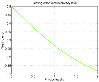
Figure 3: For any $\alpha$-DLP view $Z$ of $X$, the probability of error $P_{\mbox{\tiny{err}}}$ in distinguishing between the two hypotheses $\{X=x\}$ and $\{X=x^{\prime}\}$ is lower bounded as $P_{\mbox{\tiny{err}}}\geq\frac{1}{1+e^{\alpha}}$. Thus, for $\alpha\in[0,\frac{1}{4}]$, we are guaranteed that $P_{\mbox{\tiny{err}}}\geq 0.43$.

As Wasserman and Zhou [56] discuss, one intuitive interpretation of differential privacy is in terms of disclosure risk. More concretely, suppose that given an $\alpha$-private view $Z$ of the random variable $X$, our goal is to distinguish between the two hypotheses $\{X=x\}$ versus $\{X=x^{\prime}\}$, where $x,x^{\prime}\in\mathcal{X}$ are two distinct possible values in the sample space. A calculation shows that the best possible probability of error of any hypothesis test, with equal weights for each hypothesis, satisfies

$$P_{\mbox{\tiny{err}}}:=\frac{1}{2}\cdot\inf_{\psi}\left\{\mathbb{P}(\psi(Z)\neq x\mid X=x)+\mathbb{P}(\psi(Z)\neq x^{\prime}\mid X=x^{\prime})\right\}\geq\frac{1}{1+e^{\alpha}}.$$

Consequently, small values of $\alpha$ ensure that the performance of any test is close to random guessing (see Figure 3). We relate this in passing to Warner’s classical randomized response mechanism [55] in a simple scenario with $X\in\{0,1\}$, where we set $Z=X$ with probability $q_{\alpha}=\frac{e^{\alpha}}{1+e^{\alpha}}$, and $Z=1-X$ otherwise. Then $Q(Z=z\mid X=x)/Q(Z=z\mid X=x^{\prime})\in[e^{-\alpha},e^{\alpha}]$, and the disclosure risk $P_{\mbox{\tiny{err}}}$ is precisely $1/(1+e^{\alpha})$.

2.3 $\alpha$-private minimax risks

Given our definition of local differential privacy (LDP), we are now equipped to describe the notion of an $\alpha$-LDP minimax risk. For a given privacy level $\alpha>0$, let $\mathcal{Q}_{\alpha}$ denote the set of all conditional distributions have the $\alpha$-LDP property (3). For a given raw sample $\{X_{i}\}_{i=1}^{n}$, any distribution $Q\in\mathcal{Q}_{\alpha}$ produces a set of private observations $\{Z_{i}\}_{i=1}^{n}$, and we now restrict our attention to estimators $\widehat{\theta}=\widehat{\theta}(Z_{1},\ldots,Z_{n})$ that depend purely on this private sample. Doing so yields the modified minimax risk

$$\mathfrak{M}_{n}(\theta(\mathcal{P}),\Phi\circ\rho;Q) :=\inf_{\widehat{\theta}}\sup_{P\in\mathcal{P}}\mathbb{E}_{P,Q}\left[\Phi\big{(}\rho(\widehat{\theta}(Z_{1},\ldots,Z_{n}),\theta(P))\big{)}\right],$$ (5)

where our notation reflects the dependence on the choice of privacy mechanism $Q$. By definition, any choice of $Q\in\mathcal{Q}_{\alpha}$ guarantees that the data $\{Z_{i}\}_{i=1}^{n}$ are $\alpha$-locally differentially private, so that it is natural to seek the mechanism(s) in $\mathcal{Q}_{\alpha}$ that lead to the smallest values of the minimax risk (5). This minimization problem leads to the central object of study for this paper, a functional which characterizes the optimal rate of estimation in terms of the privacy parameter $\alpha$.

Definition 2.

Given a family of distributions $\theta(\mathcal{P})$ and a privacy parameter $\alpha>0$, the $\alpha$-private minimax risk in the metric $\rho$ is

$$\mathfrak{M}_{n}(\theta(\mathcal{P}),\Phi\circ\rho,\alpha) :=\inf_{Q\in\mathcal{Q}_{\alpha}}\inf_{\widehat{\theta}}\sup_{P\in\mathcal{P}}\mathbb{E}_{P,Q}\left[\Phi(\rho(\widehat{\theta}(Z_{1},\ldots,Z_{n}),\theta(P)))\right].$$ (6)

Note that as $\alpha\rightarrow+\infty$, the constraint of membership in $\mathcal{Q}_{\alpha}$ becomes vacuous, so that the $\alpha$-private minimax risk reduces to the classical minimax risk (1). Of primary interest in this paper are settings in which $\alpha\in\left({0},{1}\right]$, corresponding to reasonable levels of the disclosure risk, as illustrated in Figure 3.

3 Bounds on pairwise divergences: Le Cam’s bound and variants

Perhaps the oldest approach to bounding the classical minimax risk (1) is via Le Cam’s method [38]. Beginning with this technique, we develop a private analogue of the Le Cam bound, and we show how it can be used to derive sharp lower bounds on the $\alpha$-private minimax risk for one-dimensional mean and median estimation problems. We also provide new optimal procedures for each of these settings.

3.1 A private version of Le Cam’s bound

The classical version of Le Cam’s method bounds the (non-private) minimax risk (1) in terms of a two-point hypothesis testing problem [38, 58, 54]. For any distribution $P$, we use $P^{n}$ to denote the product distribution corresponding to a collection of $n$ i.i.d. samples. Let us say that a pair of distributions $\{P_{1},P_{2}\}$ is $2\delta$-separated with respect to $\theta$ if $\rho(\theta(P_{1}),\theta(P_{2}))\geq 2\delta$. With this terminology, a simple version of Le Cam’s lemma asserts that, for any $2\delta$-separated pair of distributions, the classical minimax risk has lower bound

$$\mathfrak{M}_{n}(\theta(\mathcal{P}),\Phi\circ\rho)\geq\frac{\Phi(\delta)}{2}\;\Big{\{}1-\left\|{P_{1}^{n}-P_{2}^{n}}\right\|_{\rm TV}\Big{\}}\;\stackrel{{\scriptstyle(i)}}{{\geq}}\;\frac{\Phi(\delta)}{2}\;\Big{\{}1-\frac{1}{\sqrt{2}}\sqrt{nD_{\rm kl}\left({P_{1}}\|{P_{2}}\right)}\Big{\}}.$$ (7)

Here the bound (i) follows as a consequence of the Pinsker bound on the total variation norm in terms of the KL divergence,

$$\left\|{P_{1}^{n}-P_{2}^{n}}\right\|_{\rm TV}^{2}\leq\frac{1}{2}D_{\rm kl}\left({P_{1}^{n}}\|{P_{2}^{n}}\right),$$

along with the fact $D_{\rm kl}\left({P_{1}^{n}}\|{P_{2}^{n}}\right)=nD_{\rm kl}\left({P_{1}}\|{P_{2}}\right)$ because $P_{1}^{n}$ and $P_{2}^{n}$ are product distributions (i.e., we have $X_{i}\stackrel{{\scriptstyle\rm iid}}{{\sim}}P$).

Let us now state a version of Le Cam’s lemma that applies to the $\alpha$-locally private setting in which the estimator $\widehat{\theta}$ depends only on the private variables $(Z_{1},\ldots,Z_{n})$, and our goal is to lower bound the $\alpha$-private minimax risk (6).

Proposition 1 (Private form of Le Cam bound).

Suppose that we are given $n$ i.i.d. observations from an $\alpha$-locally differential private channel for some $\alpha\in[0,\frac{23}{35}]$. Then for any pair of distributions $(P_{1},P_{2})$ that is $2\delta$-separated w.r.t. $\theta$, the $\alpha$-private minimax risk has lower bound

$$\mathfrak{M}_{n}(\theta(\mathcal{P}),\Phi\circ\rho,\alpha) \geq\frac{\Phi(\delta)}{2}\;\Big{\{}1-\sqrt{4\alpha^{2}n\left\|{P_{1}-P_{2}}\right\|_{\rm TV}^{2}}\Big{\}}\;\geq\;\frac{\Phi(\delta)}{2}\;\Big{\{}1-\sqrt{2\alpha^{2}nD_{\rm kl}\left({P_{1}}\|{P_{2}}\right)}\Big{\}}.$$ (8)

Remarks:

A comparison with the original Le Cam bound (7) shows that for $\alpha\in[0,\frac{23}{35}]$, the effect of $\alpha$-local differential privacy is to reduce the effective sample size from $n$ to at most $4\alpha^{2}n$. Proposition 1 is a corollary of more general results, which we describe in Section 3.3, that quantify the contraction in KL divergence that arises from passing the data through an $\alpha$-private channel. We also note that here—and in all subsequent bounds in the paper—we may replace the term $\alpha^{2}$ with $(e^{\alpha}-1)^{2}$, which are of the same order for $\alpha=\mathcal{O}(1)$, while the latter substitution always applies.

3.2 Some applications of the private Le Cam bound

We now turn to some applications of the $\alpha$-private version of Le Cam’s inequality from Proposition 1. First, we study the problem of one-dimensional mean estimation. In addition to demonstrating how the minimax rate changes as a function of $\alpha$, we also reveal some interesting (and perhaps disturbing) effects of enforcing $\alpha$-local differential privacy: the effective sample size may be even polynomially smaller than $\alpha^{2}n$. Our second example studies median estimation, which—as a more robust quantity than the mean—allows us to always achieve parametric convergence rates with an effective sample size reduction of $n$ to $\alpha^{2}n$. Our third example investigates conditional probability estimation, which exhibits a more nuanced dependence on privacy than the preceding estimates. We state each of our bounds assuming $\alpha\in[0,1]$; the bounds hold (with different numerical constants) whenever $\alpha\in[0,C]$ for some universal constant $C$.

3.2.1 One-dimensional mean estimation

Given a real number $k>1$, consider the family

$$\mathcal{P}_{k}:=\big{\{}\mbox{distributions $P$ such that}~{}\mathbb{E}_{P}[X]\in[-1,1]~{}\mbox{and}~{}\mathbb{E}_{P}[|X|^{k}]\leq 1\big{\}}.$$

Note that the parameter $k$ controls the tail behavior of the random variable $X$, with larger values of $k$ imposing more severe constraints. As $k\uparrow+\infty$, the random variable converges to one that is supported almost surely on the interval $[-1,1]$. Suppose that our goal is to estimate the mean $\theta(P)=\mathbb{E}_{P}[X]$, and that we adopt the squared error to measure the quality of an estimator. The classical minimax risk for this problem scales as $n^{-\min\{1,2-\frac{2}{k}\}}$ for all values of $k\geq 1$. Our goal here is to understand how the $\alpha$-private minimax risk (6),

$$\mathfrak{M}_{n}(\theta(\mathcal{P}_{k}),(\cdot)^{2},\alpha):=\inf_{Q\in\mathcal{Q}_{\alpha}}\inf_{\widehat{\theta}}\sup_{P\in\mathcal{P}_{k}}\mathbb{E}\left[\big{(}\widehat{\theta}(Z_{1},\ldots,Z_{n})-\theta(P)\big{)}^{2}\right],$$

differs from the classical minimax risk.

Corollary 1.

There exist universal constants $0<c_{\ell}\leq c_{u}\leq 9$ such that for all $k>1$ and $\alpha\in[0,1]$, the $\alpha$-minimax risk $\mathfrak{M}_{n}(\theta(\mathcal{P}_{k},(\cdot)^{2},\alpha)$ is sandwiched as

$$c_{\ell}\min\bigg{\{}1,\left(n\alpha^{2}\right)^{-\frac{k-1}{k}}\bigg{\}}\;\leq\;\mathfrak{M}_{n}(\theta(\mathcal{P}_{k}),(\cdot)^{2},\alpha)\;\leq\;c_{u}\min\left\{1,\left(n\alpha^{2}\right)^{-\frac{k-1}{k}}\right\}.$$ (9)

We prove the lower bound using the $\alpha$-private version (8) of Le Cam’s inequality from Proposition 1; see Appendix B.1 for the details.

In order to understand the bound (9), it is worthwhile considering some special cases, beginning with the usual setting of random variables with finite variance ($k=2$). In the non-private setting in which the original sample $(X_{1},\ldots,X_{n})$ is observed, the sample mean $\widehat{\theta}=\frac{1}{n}\sum_{i=1}^{n}X_{i}$ has mean-squared error at most $1/n$. When we require $\alpha$-local differential privacy, Corollary 1 shows that the minimax rate worsens to $1/\sqrt{n\alpha^{2}}$. More generally, for any $k>1$, the minimax rate scales as $\mathfrak{M}_{n}(\theta(\mathcal{P}_{k}),(\cdot)^{2},\alpha)\asymp(n\alpha^{2})^{-\frac{k-1}{k}}$. As $k\uparrow\infty$, the moment condition $\mathbb{E}[|X|^{k}]\leq 1$ becomes equivalent to the boundedness constraint $|X|\leq 1$ a.s., and we obtain the more standard parametric rate $(n\alpha^{2})^{-1}$, where there is no reduction in the exponent.

The upper bound is achieved by a variety of privacy mechanisms and estimators. One of them is the following variant of the Laplace mechanism:

• Letting $\left[{x}\right]_{T}=\max\{-T,\min\{x,T\}\}$ denote the projection of $x$ to the interval $[-T,T]$, output the private samples

  $$Z_{i}=\left[{X_{i}}\right]_{T}+W_{i},~{}~{}\mbox{where}~{}~{}W_{i}\stackrel{{\scriptstyle\rm iid}}{{\sim}}\mathop{\rm Laplace}(\alpha/(2T))~{}~{}\mbox{and}~{}T=(n\alpha^{2})^{\frac{1}{2k}}.$$ (10)

• Compute the sample mean $\widehat{\theta}_{n}:=\frac{1}{n}\sum_{i=1}^{n}Z_{i}$ of the privatized data.

We present the analysis of this estimator in Appendix B.1. It is one case in which the widely-used Laplacian mechanism is an optimal mechanism; later examples show that this is not always the case.

Summarizing our results thus far, Corollary 1 helps to demarcate situations in which local differential privacy may or may not be acceptable for location estimation problems. In particular, for bounded domains—where we may take $k\uparrow\infty$—local differential privacy may be quite reasonable. However, in situations in which the sample takes values in an unbounded space, local differential privacy imposes more severe constraints.

3.2.2 One-dimensional median estimation

Instead of attempting to privately estimate the mean—an inherently non-robust quantity—we may also consider median estimation problems. Median estimation for general distributions is impossible even in non-private settings, so we focus on the median as an $M$-estimator. Recalling that the minimizer(s) of $\mathbb{E}[|X-\theta|]$ are the median(s) of $X$, we consider the gap between mean absolute error of our estimator and that of the true median,

$$\mathbb{E}[R(\widehat{\theta})]-\inf_{\theta\in\mathbb{R}}R(\theta),~{}~{}\mbox{where}~{}~{}R(\theta):=\mathbb{E}[|X-\theta|].$$

We first give a proposition characterizing the minimax rate for this problem by applying Proposition 1. Let $\theta(P)=\mathop{\rm med}(P)$ denote the median of the distribution $P$, and for radii $r>0$, we consider the family of distributions supported on $\mathbb{R}$ defined by

$$\mathcal{P}_{r}:=\left\{\mbox{distributions}~{}P~{}\mbox{such that}~{}|\mathop{\rm med}(P)|\leq r,~{}\mathbb{E}_{P}[|X|]<\infty\right\}.$$

In this case, we consider the slight variant of the minimax rate (6) defined by the risk gap

$$\mathfrak{M}_{n}(\theta(\mathcal{P}_{r}),R,\alpha):=\inf_{Q\in\mathcal{Q}_{\alpha}}\inf_{\widehat{\theta}}\sup_{P\in\mathcal{P}_{r}}\mathbb{E}_{P,Q}\left[R(\widehat{\theta}(Z_{1},\ldots,Z_{n}))-R(\theta(P))\right].$$

We then have the following.

Corollary 2.

For the median estimation problem, there are universal constants $\frac{1}{20}\leq c_{\ell}\leq c_{u}<6$ such that for all $r\geq 0$ and $\alpha\in[0,1]$, the minimax error satisfies

$$c_{\ell}\cdot r\min\left\{1,(n\alpha^{2})^{-\frac{1}{2}}\right\}\leq\mathfrak{M}_{n}(\theta(\mathcal{P}_{r}),R,\alpha)\leq c_{u}\cdot r\min\left\{1,(n\alpha^{2})^{-\frac{1}{2}}\right\}.$$

We present the proof of the lower bound in Corollary 2 to Section B.2, focusing our attention here on a minimax optimal sequential procedure based on stochastic gradient descent (SGD).

To describe our SGD procedure, let $\theta_{0}\in[-r,r]$ be arbitrary, and $W_{i}$ be an i.i.d. $\{-1,+1\}$ Bernoulli sequence with $\mathbb{P}(W_{i}=1)=\frac{e^{\alpha}}{e^{\alpha}+1}$, and let $X_{i}\stackrel{{\scriptstyle\rm iid}}{{\sim}}P$ be the observations of the distribution $P$ whose median we wish to estimate (and which must be made private). We iterate according to the projected stochastic gradient descent procedure

$$\theta_{i+1}=\left[{\theta_{i}-\eta_{i}Z_{i}}\right]_{r},~{}~{}\mbox{where}~{}~{}Z_{i}=\frac{e^{\alpha}+1}{e^{\alpha}-1}\cdot W_{i}\cdot\mathop{\rm sign}(\theta_{i}-X_{i}),$$ (11)

where as in expression (10), $\left[{x}\right]_{r}=\max\{-r,\min\{x,r\}\}$ is the projection onto the set $[-r,r]$, and the sequence $\eta_{i}>0$ are non-increasing stepsizes. By inspection we see that $Z_{i}$ is differentially private for $X_{i}$, and we have the conditional unbiasedness $\mathbb{E}[Z_{i}\mid X_{i},\theta_{i}]=\mathop{\rm sign}(\theta_{i}-X_{i})\in\partial_{\theta}|\theta_{i}-X_{i}|$, where $\partial$ denotes the subdifferential operator. Standard results on stochastic gradient descent methods [45] imply that for $\widehat{\theta}_{n}=\frac{1}{n}\sum_{i=1}^{n}\theta_{i}$, we have

$$\mathbb{E}[R(\widehat{\theta}_{n})]-\inf_{\theta\in[-r,r]}R(\theta)\leq\frac{1}{n}\left[\frac{r^{2}}{\eta_{n}}+\frac{1}{2}\sum_{i=1}^{n}\eta_{i}\left(\frac{e^{\alpha}+1}{e^{\alpha}-1}\right)^{2}\right].$$

Under the assumption that $\alpha\leq 1$, we take $\eta_{i}=\alpha\cdot r/\sqrt{i}$, which immediately implies the upper bound $\mathbb{E}[R(\widehat{\theta}_{n})]-R(\mathop{\rm med}(P))\leq\frac{6r}{\sqrt{n\alpha^{2}}}$.

We make two remarks on the procedure (11). First, it is essentially a sequential variant of Warner’s 1965 randomized response [55], a procedure whose variants turn out to often be optimal, as we show in the sequel. Secondly, while at first blush it is not clear that the additional complexity of stochastic gradient descent is warranted, we provide experiments comparing the SGD procedure with more naive estimators in Section 6.1.2 on a salary estimation task. These experiments corroborate the improved performance of our minimax optimal strategy.

3.3 Pairwise upper bounds on Kullback-Leibler divergences

As mentioned previously, the private form of Le Cam’s bound (Proposition 1) is a corollary of more general results on the contractive effects of privacy on pairs of distributions, which we now state. Given a pair of distributions $(P_{1},P_{2})$ defined on a common space $\mathcal{X}$, any conditional distribution $Q$ transforms such a pair of distributions into a new pair $(M_{1},M_{2})$ via the marginalization operation $M_{j}(S)=\int_{\mathcal{X}}Q(S\mid x)dP_{j}(x)$ for $j=1,2$. Intuitively, when the conditional distribution $Q$ is $\alpha$-locally differentially private, the two output distributions $(M_{1},M_{2})$ should be closer together. The following theorem makes this intuition precise:

Theorem 1.

For any $\alpha\geq 0$, let $Q$ be a conditional distribution that guarantees $\alpha$-differential privacy. Then, for any pair of distributions $P_{1}$ and $P_{2}$, the induced marginals $M_{1}$ and $M_{2}$ satisfy the bound

$$D_{\rm kl}\left({M_{1}}\|{M_{2}}\right)+D_{\rm kl}\left({M_{2}}\|{M_{1}}\right)\leq\min\{4,e^{2\alpha}\}(e^{\alpha}-1)^{2}\left\|{P_{1}-P_{2}}\right\|_{\rm TV}^{2}.$$ (12)

Remarks:

Theorem 1 is a type of strong data processing inequality [2], providing a quantitative relationship between the divergence $\left\|{P_{1}-P_{2}}\right\|_{\rm TV}$ and the KL-divergence $D_{\rm kl}\left({M_{1}}\|{M_{2}}\right)$ that arises after applying the channel $Q$. The result of Theorem 1 is similar to a result due to Dwork, Rothblum, and Vadhan [22, Lemma III.2], who show that $D_{\rm kl}\left({Q(\cdot\mid x)}\|{Q(\cdot\mid x^{\prime})}\right)\leq\alpha(e^{\alpha}-1)$ for any $x,x^{\prime}\in\mathcal{X}$, which implies $D_{\rm kl}\left({M_{1}}\|{M_{2}}\right)\leq\alpha(e^{\alpha}-1)$ by convexity. This upper bound is weaker than Theorem 1 since it lacks the term $\left\|{P_{1}-P_{2}}\right\|_{\rm TV}^{2}$. This total variation term is essential to our minimax lower bounds: more than providing a bound on KL divergence, Theorem 1 shows that differential privacy acts as a contraction on the space of probability measures. This contractivity holds in a strong sense: indeed, the bound (12) shows that even if we start with a pair of distributions $P_{1}$ and $P_{2}$ whose KL divergence is infinite, the induced marginals $M_{1}$ and $M_{2}$ always have finite KL divergence. We provide the proof of Theorem 1 in Appendix A.

Let us now develop a corollary of Theorem 1 that has a number of useful consequences, among them the private form of Le Cam’s method from Proposition 1. Suppose that we are given an indexed family of distributions $\{P_{\nu},\nu\in\mathcal{V}\}$. Let $V$ denote a random variable that is uniformly distributed over the finite index set $\mathcal{V}$. Conditionally on $V=\nu$, suppose we sample a random vector $(X_{1},\ldots,X_{n})$ according to a product measure of the form $P_{\nu}(x_{1},\ldots,x_{n}):=\prod_{i=1}^{n}P_{\nu(i)}(x_{i})$, where $(\nu(1),\ldots,\nu(n))$ denotes some sequence of indices. Now suppose that we draw an $\alpha$-locally private sample $(Z_{1},\ldots,Z_{n})$ according to the channel $Q(\cdot\mid X_{1:n})$. Conditioned on $V=\nu$, the private sample is distributed according to the measure $M_{\nu}^{n}$ given by

$$M_{\nu}^{n}(S):=\int Q^{n}(S\mid x_{1},\ldots,x_{n})dP_{\nu}(x_{1},\ldots,x_{n})~{}~{}~{}\mbox{for}~{}S\in\sigma(\mathcal{Z}^{n}).$$ (13)

Since we allow interactive protocols, the distribution $M_{\nu}^{n}$ need not be a product distribution in general. Nonetheless, in this setup we have the following tensorization inequality:

Corollary 3.

For any $\alpha$-locally differentially private conditional distribution (3) $Q$ and any paired sequences of distributions $\{P_{\nu(i)}\}$ and $\{P_{{\nu^{\prime}}(i)}\}$, we have

$$D_{\rm kl}\left({M_{\nu}^{n}}\|{M_{{\nu^{\prime}}}^{n}}\right) \leq 4(e^{\alpha}-1)^{2}\sum_{i=1}^{n}\left\|{P_{\nu(i)}-P_{{\nu^{\prime}}(i)}}\right\|_{\rm TV}^{2}.$$ (14)

See Appendix A.2 for the proof, which requires a few intermediate steps to obtain the additive inequality. One consequence of Corollary 3 is the private form of Le Cam’s bound in Proposition 1. Given the index set $\mathcal{V}=\{1,2\}$, consider two paired sequences of distributions of the form $\{P_{1},\ldots,P_{1}\}$ and $\{P_{2},\ldots,P_{2}\}$. With this choice, we have

$$\left\|{M_{1}^{n}-M_{2}^{n}}\right\|_{\rm TV}^{2} \stackrel{{\scriptstyle(i)}}{{\leq}}\frac{1}{2}D_{\rm kl}\left({M_{1}^{n}}\|{M_{2}^{n}}\right)\;\stackrel{{\scriptstyle(ii)}}{{\leq}}\;2(e^{\alpha}-1)^{2}n\left\|{P_{1}-P_{2}}\right\|_{\rm TV},$$

where step (i) is Pinsker’s inequality, and step (ii) follows from the tensorization inequality (14) and the i.i.d. nature of the product distributions $P_{1}^{n}$ and $P_{2}^{n}$. Noting that $(e^{\alpha}-1)^{2}\leq 2\alpha^{2}$ for $\alpha\leq\frac{23}{35}$ and applying the classical Le Cam bound (7) gives Proposition 1.

In addition, inequality (14) can be used to derive a bound on the mutual information. Bounds of this type are useful in applications of Fano’s method, to be discussed at more length in the following section. In particular, if we define the mixture distribution $\overline{M}^{n}=\frac{1}{|\mathcal{V}|}\sum_{\nu\in\mathcal{V}}M^{n}_{\nu}$, then by the definition of mutual information, we have

$$I(Z_{1},\ldots,Z_{n};V)\;=\;\frac{1}{|\mathcal{V}|}\sum_{\nu\in\mathcal{V}}D_{\rm kl}\left({M_{\nu}^{n}}\|{\overline{M}^{n}}\right) \leq\frac{1}{|\mathcal{V}|^{2}}\sum_{\nu,{\nu^{\prime}}}D_{\rm kl}\left({M_{\nu}^{n}}\|{M_{{\nu^{\prime}}}^{n}}\right)$$

$$\leq 4(e^{\alpha}-1)^{2}\sum_{i=1}^{n}\frac{1}{|\mathcal{V}|^{2}}\sum_{\nu,{\nu^{\prime}}\in\mathcal{V}}\left\|{P_{\nu(i)}-P_{{\nu^{\prime}}(i)}}\right\|_{\rm TV}^{2},$$ (15)

the first inequality following from the joint convexity of the KL divergence and the final inequality from Corollary 3.

Remarks:

Mutual information bounds under local privacy have appeared previously. McGregor et al. [43] study relationships between communication complexity and differential privacy, showing that differentially private schemes allow low communication. They provide a result [43, Prop. 7] guaranteeing $I(X_{1:n};Z_{1:n})\leq 3\alpha n$; they strengthen this bound to $I(X_{1:n};Z_{1:n})\leq(3/2)\alpha^{2}n$ when the $X_{i}$ are i.i.d. uniform Bernoulli variables. Since the total variation distance is at most $1$, our result also implies this scaling (for arbitrary $X_{i}$); however, our result is stronger since it involves the total variation terms $\|{P_{\nu(i)}-P_{{\nu^{\prime}}(i)}}\|_{\rm TV}$. These TV terms are an essential part of obtaining the sharp minimax results that are our focus. In addition, Corollary 3 allows for any sequentially interactive channel $Q$; each random variable $Z_{i}$ may depend on the private answers $Z_{1:i-1}$ of other data providers.

4 Bounds on private mutual information: Fano’s method

We now turn to a set of techniques for bounding the private minimax risk (6) based on Fano’s inequality from information theory. We begin by describing how Fano’s inequality is used in classical minimax theory, then presenting some of its extensions to the private setting.

Recall that our goal is to lower bound the minimax risk associated with estimating some parameter $\theta(P)$ in a given metric $\rho$. Given a finite set $\mathcal{V}$, a family of distributions $\{P_{\nu},\nu\in\mathcal{V}\}$ is said to be $2\delta$-separated in the metric $\rho$ if $\rho(\theta(P_{\nu}),\theta(P_{\nu^{\prime}}))\geq 2\delta$ for all distinct pairs $\nu,{\nu^{\prime}}\in\mathcal{V}$. Given any such $2\delta$-separated set, the classical form of Fano’s inequality [cf. 58] asserts that the minimax risk (1) has lower bound

$$\mathfrak{M}_{n}(\theta(\mathcal{P}),\Phi\circ\rho) \geq\frac{\Phi(\delta)}{2}\left\{1-\frac{I(V;X_{1}^{n})+\log 2}{\log|\mathcal{V}|}\right\}.$$

Here $I(V;X_{1}^{n})$ denotes the mutual information between a random variable $V$ uniformly distributed over the set $\mathcal{V}$ and a random vector $X_{1}^{n}=(X_{1},\ldots,X_{n})$ drawn from the mixture distribution

$$\overline{P}:=\frac{1}{|\mathcal{V}|}\sum_{\nu\in\mathcal{V}}P^{n}_{\nu},$$ (16)

so that $I(V;X_{1}^{n})=\frac{1}{|\mathcal{V}|}\sum_{\nu}D_{\rm kl}\left({P^{n}_{\nu}}\|{\overline{P}}\right)$; equivalently, the random variables are drawn $X_{i}\stackrel{{\scriptstyle\rm iid}}{{\sim}}P_{\nu}$ conditional on $V=\nu$. In the cases we consider, it is sometimes convenient to use a slight generalization of the classical Fano method by extending the $2\delta$-separation above. Let $\rho_{\mathcal{V}}$ be a metric on the set $\mathcal{V}$, and for $t\geq 0$ define the neighborhood size for the set $\mathcal{V}$ by

$$N_{t}:=\max_{\nu\in\mathcal{V}}\mathop{\rm card}\left\{{\nu^{\prime}}\in\mathcal{V}\mid\rho_{\mathcal{V}}(\nu,{\nu^{\prime}})\leq t\right\}$$ (17)

and the separation function

$$\delta(t):=\frac{1}{2}\min\left\{\rho(\theta(P_{\nu}),\theta(P_{\nu^{\prime}}))\mid\nu,{\nu^{\prime}}\in\mathcal{V}~{}\mbox{and}~{}\rho_{\mathcal{V}}(\nu,{\nu^{\prime}})>t\right\}.$$ (18)

Then we have the following generalization [14, Corollary 1] of the Fano bound: for any $t\geq 0$,

$$\mathfrak{M}_{n}(\theta(\mathcal{P}),\Phi\circ\rho)\geq\frac{\Phi(\delta(t))}{2}\left\{1-\frac{I(V;X_{1}^{n})+\log 2}{\log|\mathcal{V}|-\log N_{t}}\right\}.$$ (19)

4.1 A private version of Fano’s method

We now turn to developing a version of Fano’s lower bound that applies to estimators $\widehat{\theta}$ that act on privatized samples $Z_{1}^{n}=(Z_{1},\ldots,Z_{n})$, where the obfuscation channel $Q$ is non-interactive (Figure 2(b)), meaning that $Z_{i}$ is conditionally independent of $Z_{\setminus i}$ given $X_{i}$. Our upper bound is variational: it involves optimization over a subset of the space $L^{\infty}(\mathcal{X}):=\big{\{}f:\mathcal{X}\rightarrow\mathbb{R}\,\mid\,\|f\|_{\infty}<\infty\big{\}}$ of uniformly bounded functions equipped with the supremum norm $\left\|{f}\right\|_{\infty}=\sup_{x}|f(x)|$ and the associated $1$-ball of the supremum norm

$$\mathbb{B}_{\infty}(\mathcal{X}):=\left\{\gamma\in L^{\infty}(\mathcal{X})\mid\|\gamma\|_{\infty}\leq 1\right\}.$$ (20)

As the set $\mathcal{X}$ is generally clear from context, we typically omit this dependence (and adopt the shorthand $\mathbb{B}_{\infty}$). As with the classical Fano method, we consider a $2\delta$-separated family of distributions $\{P_{\nu},\nu\in\mathcal{V}\}$, and for each $\nu\in\mathcal{V}$, we define the linear functional $\varphi_{\nu}:L^{\infty}(\mathcal{X})\rightarrow\mathbb{R}$ by

$$\varphi_{\nu}(\gamma)=\int_{\mathcal{X}}\gamma(x)(dP_{\nu}(x)-d\overline{P}(x)).$$ (21)

With this notation, we have the following private version of Fano’s method:

Proposition 2 (Private Fano method).

Given any set $\{P_{\nu},\nu\in\mathcal{V}\}$, for any $t\geq 0$ the non-interactive $\alpha$-private minimax risk has lower bound

$$\mathfrak{M}_{n}(\theta(\mathcal{P}),\Phi\circ\rho,\alpha) \geq\frac{\Phi(\delta(t))}{2}\;\left\{1-\frac{n(e^{\alpha}-1)^{2}}{\log(|\mathcal{V}|/N_{t})}\bigg{[}\frac{1}{|\mathcal{V}|}\sup_{\gamma\in\mathbb{B}_{\infty}}\sum_{\nu\in\mathcal{V}}\left(\varphi_{\nu}(\gamma)\right)^{2}\bigg{]}-\frac{\log 2}{\log(|\mathcal{V}|/N_{t})}\right\}.$$

Underlying Proposition 2 is a variational bound on the mutual information between a sequence $Z_{1}^{n}=(Z_{1},\ldots,Z_{n})$ of private random variables and a random index $V$ drawn uniformly on $\mathcal{V}$, where $Z_{1}^{n}\sim M_{\nu}^{n}$, conditional on $V=\nu$; that is, $Z_{1}^{n}$ is marginally drawn according to the mixture

$$\overline{M} :=\frac{1}{|\mathcal{V}|}\sum_{\nu\in\mathcal{V}}M_{\nu}^{n}~{}~{}\mbox{where}~{}M^{n}_{\nu}(S)=\int Q(S\mid x_{1}^{n})dP^{n}_{\nu}(x_{1}^{n}).$$

(Recall equation (13)). When the conditional distribution $Q$ is non-interactive, as considered in this section, then $M^{n}_{\nu}$ is also a product distribution. By comparison with equation (16), we see that $\overline{M}$ is the private analogue of the mixture distribution $\overline{P}$ that arises in the classical Fano analysis.

Proposition 2 is an immediate consequence of the Fano bound (19) coupled with the following upper bound on the mutual information between $Z_{1}^{n}$ and an index $V$ uniformly distributed over $\mathcal{V}$:

$$I(V;Z_{1}^{n}) \leq n(e^{\alpha}-1)^{2}\frac{1}{|\mathcal{V}|}\sup_{\gamma\in\mathbb{B}_{\infty}}\sum_{\nu\in\mathcal{V}}\left(\varphi_{\nu}(\gamma)\right)^{2}.$$ (22)

The inequality (22) is in turn an immediate consequence of Theorem 2 to come; we provide the proof of this inequality in Appendix C.2. We conjecture that it also holds in the fully interactive setting, but given well-known difficulties of characterizing multiple channel capacities with feedback [13, Chapter 15], it may be challenging to verify this conjecture.

4.2 Some applications of the private Fano bound

In this section, we show how Proposition 2 leads to sharp characterizations of the $\alpha$-private minimax rates for some classical and high-dimensional mean estimation problems. We consider estimation of the $d$-dimensional mean $\theta(P):=\mathbb{E}_{P}[X]$ of a random vector $X\in\mathbb{R}^{d}$. Due to the difficulties associated with differential privacy on non-compact spaces (recall Section 3.2.1), we focus on distributions with compact support. We provide proofs of our mean estimation results in Appendix D.

4.2.1 Classical mean estimation in $d$ dimensions

We begin by considering estimation of means for sampling distributions supported on $\ell_{p}$ balls, where $p\in[1,2]$. Indeed, for a radius $r<\infty$, consider the family

$$\mathcal{P}_{p,r} :=\big{\{}\mbox{distributions~{}}P~{}\mbox{supported on}~{}\mathbb{B}_{p}(r)\subset\mathbb{R}^{d}\big{\}},$$

where $\mathbb{B}_{p}(r)=\{x\in{}^{d}\mid\left\|{x}\right\|_{p}\leq r\}$ is the $\ell_{p}$-ball of radius $r$. In the non-private setting, the standard estimator $\widehat{\theta}=\frac{1}{n}\sum_{i=1}^{n}X_{i}$ has mean-squared error at most $r^{2}/n$, since $\left\|{X}\right\|_{2}\leq\left\|{X}\right\|_{p}\leq r$ by assumption. The following result shows that the private minimax MSE is substantially different:

Corollary 4.

For the mean estimation problem, for all $p\in[1,2]$ and privacy levels $\alpha\in[0,1]$, the non-interactive private minimax risk satisfies

$$r^{2}\min\left\{1,\max\left\{\frac{1}{\sqrt{n\alpha^{2}}}\wedge\frac{d}{n\alpha^{2}},\frac{1}{(n\alpha^{2})^{\frac{2-p}{p}}}\wedge\frac{d^{2\frac{p-1}{p}}}{n\alpha^{2}}\right\}\right\}\lesssim\mathfrak{M}_{n}(\theta(\mathcal{P}_{p,r}),\left\|{\cdot}\right\|_{2}^{2},\alpha)\lesssim r^{2}\min\left\{\frac{d}{n\alpha^{2}},1\right\}.$$

See Appendix D.1 for the proof of this claim; the lower bound makes use of the private form of Fano’s method (Proposition 2), while the upper bound is a consequence of the optimal mechanisms we develop in Section 4.2.3.

Corollary 4 demonstrates the substantial difference between $d$-dimensional mean estimation in private and non-private settings: the privacy constraint leads to a multiplicative penalty of $d/\alpha^{2}$ in terms of mean-squared error. Thus, the effect of privacy is to reduce the effective sample size from $n$ to $\alpha^{2}n/d$. We remark in passing that if $\alpha\geq 1$, our result still holds, though we replace the quantity $\alpha$ in the lower bound with the quantity $e^{\alpha}-1$ and in the upper bound with $1-e^{-\alpha}$. The lower bound as written is somewhat complex in its dependence on $p\in[1,2]$, so an investigation of the extreme cases is somewhat helpful. Taking $p=2$, the scaling in the lower bound simplifies to $\min\{1,\frac{d}{n\alpha^{2}}\}$, identical to the upper bound; in the case $p=1$, it becomes $\min\{1,\frac{1}{\sqrt{n\alpha^{2}}},\frac{d}{n\alpha^{2}}\}$. There is a gap in the regime $d\geq\sqrt{n\alpha^{2}}$ in this case, though the asymptotic regime for large $n$ shows that both the lower and upper bounds become $d/(n\alpha^{2})$, independent of $p\in[1,2]$.

4.2.2 Estimation of high-dimensional sparse vectors

Recently, there has been substantial interest in high-dimensional problems in which the dimension $d$ is larger than the sample size $n$, but a low-dimensional latent structure makes inference possible [10, 44]. Here we consider a simple but canonical instance of a high-dimensional problem, that of estimating a sparse mean vector. For an integer parameter $s\geq 1$, consider the class of distributions

$$\mathcal{P}_{\infty,r}^{s}:=\left\{\mbox{distributions}~{}P~{}\mbox{supported~{}on~{}}\mathbb{B}_{\infty}(r)\subset\mathbb{R}^{d}~{}\mbox{with~{}}\left\|{\mathbb{E}_{P}[X]}\right\|_{0}\leq s\right\}.$$ (23)

In the non-private case, estimation of such an $s$-sparse predictor in the squared $\ell_{2}$-norm is possible at rate $\mathbb{E}[\|{\widehat{\theta}-\theta}\|_{2}^{2}]\lesssim r^{2}\frac{s\log(d/s)}{n}$, so that the dimension $d$ can be exponentially larger than the sample size $n$. With this context, the next result shows that local privacy can have a dramatic impact in the high-dimensional setting. For simplicity, we restrict ourselves to the easiest case of a $1$-sparse vector ($s=1$).

Corollary 5.

For the $1$-sparse means problem, for all $\alpha\geq 0$, the non-interactive private minimax risk satisfies

$$\min\left\{r^{2},\frac{r^{2}d\log(2d)}{n(e^{\alpha}-1)^{2}}\right\}\;\lesssim\;\mathfrak{M}_{n}\left(\theta(\mathcal{P}_{\infty,r}^{1}),\left\|{\cdot}\right\|_{2}^{2},\alpha\right)\;\lesssim\;\min\left\{r^{2},\frac{r^{2}d\log(2d)}{n(1-e^{-\alpha})^{2}}\right\}.$$

See Appendix D.2 for a proof.

From the lower bound in Corollary 5, we see that local differential privacy has an especially dramatic effect for the sparse means problem: due to the presence of the $d$-term in the numerator, estimation in high-dimensional settings ($d\geq n$) becomes impossible, even for $1$-sparse vectors. Contrasting this fact with the scaling $d\asymp e^{n}$ that $1$-sparsity allows in the non-private setting shows that local differential privacy is a very severe constraint in this setting. We note in passing that an essentially identical argument to that we provide in Appendix D.2 gives a lower bound of $r\sqrt{\frac{d\log(2d)}{n(e^{\alpha}-1)^{2}}}$ on estimation with $\left\|{\cdot}\right\|_{\infty}$ error. Corollary 5 raises the question of whether high-dimensional estimation is possible with local differential privacy. In non-interactive settings, our result shows that there is a dimension-dependent penalty that must be paid for estimation; in scenarios in which it is possible to modify the privatizing mechanism $Q$, it may be possible to “localize” in an appropriate sense once important variables have been identified, providing some recourse against the negative results of Corollary 5. We leave such considerations to future work.

4.2.3 Optimal mechanisms: attainability for mean estimation

Our lower bounds for both $d$-dimensional mean estimation (Corollary 4) and $1$-sparse mean estimation (Corollary 5) are based on the private form of Fano’s method (Proposition 2). On the other hand, the upper bounds are based on direct analysis of specific privacy mechanisms and estimators. Here we discuss the optimal privacy mechanisms for these two problems in more detail.

Sub-optimality of Laplacian mechanism:

For the $1$-dimensional mean estimation problem (Corollary 1), we showed that adding Laplacian noise to (truncated versions of) the observations led to an optimal privacy mechanism. The extension of this result to the $d$-dimensional problems considered in Corollary 4, however, fails. More concretely, as a special case of the families in Corollary 4, consider the class $\mathcal{P}_{2,1}$ of distributions supported on the Euclidean ball $\mathbb{B}_{2}(1)\subset\mathbb{R}^{d}$ of unit norm. In order to guarantee $\alpha$-differential privacy, suppose that we output the additively corrupted random vector $Z:=x+W$, where the noise vector $W\in\mathbb{R}^{d}$ has i.i.d components following a $\mathop{\rm Laplace}(\alpha/\sqrt{d})$ distribution. With this choice, it can be verified that for $X$ taking values in $\mathbb{B}_{2}(1)$, the random vector $Z$ is an $\alpha$-DLP view of $X$. However, this privacy mechanism does not achieve the minimax risk over $\alpha$-private mechanisms. In particular, one must suffer the rate

$$\inf_{\widehat{\theta}}\sup_{P\in\mathcal{P}}\mathbb{E}_{P}\left[\|{\widehat{\theta}(Z_{1},\ldots,Z_{n})-\mathbb{E}_{P}[X]}\|_{2}^{2}\right]\gtrsim\min\left\{\frac{d^{2}}{n\alpha^{2}},1\right\},$$ (24)

a quadratic ($d^{2}$) dimension dependence, as opposed to the linear scaling ($d$) of the optimal result in Corollary 4. See Appendix D.3 for the proof of claim (24). The poorer dimension dependence of the Laplacian mechanism demonstrates that sampling mechanisms must be chosen carefully.

Optimal mechanisms:

Let us now describe some mechanisms that are optimal for the $d$-dimensional and $1$-sparse mean estimation problems. Both of them are procedures that output a random variable $Z$ that is an $\alpha$-differentially-private view of $X$, and they are unbiased in the sense that $\mathbb{E}[Z\mid X=x]=x$. They require the Bernoulli random variable

$$T\sim\mathop{\rm Bernoulli}(\pi_{\alpha}),\quad\mbox{where}\quad\pi_{\alpha}:=e^{\alpha}/(e^{\alpha}+1).$$

Privacy mechanism for $\ell_{2}$-ball: Given a vector $x\in{}^{d}$ with $\left\|{x}\right\|_{2}\leq r$, define a random vector

$$\widetilde{X} :=\begin{cases}+r\frac{x}{\left\|{x}\right\|_{2}}&\mbox{ with probability $\frac{1}{2}+\frac{\left\|{x}\right\|_{2}}{2r}$}\\ -r\frac{x}{\left\|{x}\right\|_{2}}&\mbox{ with probability $\frac{1}{2}-\frac{\left\|{x}\right\|_{2}}{2r}$}.\end{cases}$$

Then sample $T\sim\mathop{\rm Bernoulli}(\pi_{\alpha})$ and set

$$Z\sim\begin{cases}\mathop{\rm Uniform}(z\in\mathbb{R}^{d}\mid\langle z,\,\widetilde{X}\rangle>0,\left\|{z}\right\|_{2}=B)&\mbox{if~{}}T=1\\ \mathop{\rm Uniform}(z\in\mathbb{R}^{d}\mid\langle z,\,\widetilde{X}\rangle\leq 0,\left\|{z}\right\|_{2}=B)&\mbox{if~{}}T=0,\end{cases}$$ (25)

where $B$ is chosen to equal

$$B=r\frac{e^{\alpha}+1}{e^{\alpha}-1}\frac{\sqrt{\pi}}{2}\frac{d\,\Gamma(\frac{d-1}{2}+1)}{\Gamma(\frac{d}{2}+1)}.$$

Privacy mechanism for $\ell_{\infty}$-ball: Given a vector $x\in{}^{d}$ with $\left\|{x}\right\|_{\infty}\leq r$, construct a random vector $\widetilde{X}\in\mathbb{R}^{d}$ with independent coordinates of the form

$$\widetilde{X}_{j} =\begin{cases}+r&\mbox{with probability $\frac{1}{2}+\frac{x_{j}}{2r}$}\\ -r&\mbox{with probability $\frac{1}{2}-\frac{x_{j}}{2r}$}.\end{cases}$$

Then sample $T\sim\mathop{\rm Bernoulli}(\pi_{\alpha})$ and set

$$Z\sim\begin{cases}\mathop{\rm Uniform}(z\in\{-B,B\}^{d}\mid\langle z,\,\widetilde{X}\rangle\geq 0)&\mbox{if~{}}T=1\\ \mathop{\rm Uniform}(z\in\{-B,B\}^{d}\mid\langle z,\,\widetilde{X}\rangle\leq 0)&\mbox{if~{}}T=0,\end{cases}$$ (26)

where the value $B$ is chosen to equal

$$B=r\frac{e^{\alpha}+1}{e^{\alpha}-1}C_{d},~{}~{}\mbox{where}~{}~{}C_{d}^{-1}=\begin{cases}\frac{1}{2^{d-1}}\binom{d-1}{(d-1)/2}&\mbox{if~{}}d~{}\mbox{is odd}\\ \frac{1}{2^{d-1}+\frac{1}{2}\binom{d}{d/2}}\binom{d-1}{d/2}&\mbox{if~{}}d~{}\mbox{is even.}\end{cases}$$

See Figure 4 for visualizations of the geometry that underlies these strategies. By construction, each scheme guarantees that $Z$ is an $\alpha$-private view of $X$. Each strategy is efficiently implementable when combined with rejection sampling: the $\ell_{2}$-mechanism (25) by normalizing a sample from the $\mathsf{N}(0,I_{d\times d})$ distribution, and the $\ell_{\infty}$-strategy (26) by sampling the hypercube $\{-1,1\}^{d}$. Additionally, by Stirling’s approximation, we have that in each case $B\lesssim\frac{r\sqrt{d}}{\alpha}$ for $\alpha\leq 1$. Moreover, they are unbiased (see Appendix I.2 for the unbiasedness of strategy (25) and Appendix I.3 for strategy (26)).

We now complete the picture of minimax optimal estimation schemes for Corollaries 4 and 5. In the case of Corollary 4, the estimator $\widehat{\theta}:=\frac{1}{n}\sum_{i=1}^{n}Z_{i}$, where $Z_{i}$ is constructed by procedure (25) from the non-private vector $X_{i}$, attains the minimax optimal convergence rate. In the case of Corollary 5, a slightly more complex estimator gives that rate: in particular, we set

$$\widehat{\theta}_{n}:=\mathop{\rm argmin}_{\theta\in\mathbb{R}^{d}}\bigg{\{}\frac{1}{2n}\sum_{i=1}^{n}\left\|{Z_{i}-\theta}\right\|_{2}^{2}+\lambda_{n}\left\|{\theta}\right\|_{1}\bigg{\}},~{}~{}~{}\mbox{where}~{}~{}\lambda_{n}=2\frac{\sqrt{d\log d}}{\sqrt{n\alpha^{2}}},$$

and the $Z_{i}$ are drawn according to strategy (26). See Appendix D.2 for a rigorous argument.

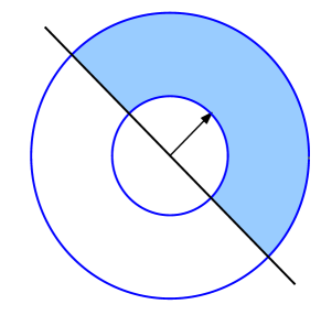
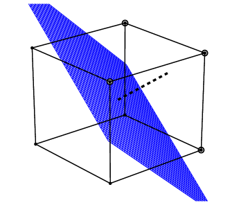
(a)		(b)

Figure 4: Private sampling strategies for different types of $\ell_{p}$-balls. (a) A private sampling strategy (25) for data lying within an $\ell_{2}$-ball. Outer boundary of highlighted region sampled uniformly with probability $e^{\alpha}/(e^{\alpha}+1)$. (b) A private sampling strategy (26) for data lying within an $\ell_{\infty}$-ball. Circled point set sampled uniformly with probability $e^{\alpha}/(e^{\alpha}+1)$.

4.3 Variational bounds on private mutual information

The private Fano bound in Proposition 2 reposes on a variational bound on the private mutual information that we describe here. Recall the space $L^{\infty}(\mathcal{X}):=\big{\{}f:\mathcal{X}\rightarrow\mathbb{R}\,\mid\,\|f\|_{\infty}<\infty\big{\}}$ of uniformly bounded functions, equipped with the usual sup-norm and unit norm ball (20), $\mathbb{B}_{\infty}$, as well as the linear functionals $\varphi_{\nu}$ from Eq. (21). We then have the following result.

Theorem 2.

Let $\{P_{\nu}\}_{\nu\in\mathcal{V}}$ be an arbitrary collection of probability measures on $\mathcal{X}$, and let $\{M_{\nu}\}_{\nu\in\mathcal{V}}$ be the set of marginal distributions induced by an $\alpha$-differentially private distribution $Q$. Then

$$\frac{1}{|\mathcal{V}|}\sum_{\nu\in\mathcal{V}}\left[D_{\rm kl}\left({M_{\nu}}\|{\overline{M}}\right)+D_{\rm kl}\left({\overline{M}}\|{M_{\nu}}\right)\right] \leq\frac{(e^{\alpha}-1)^{2}}{|\mathcal{V}|}\sup_{\gamma\in\mathbb{B}_{\infty}(\mathcal{X})}\sum_{\nu\in\mathcal{V}}\left(\varphi_{\nu}(\gamma)\right)^{2}.$$

It is important to note that, at least up to constant factors, Theorem 2 is never weaker than the results provided by Theorem 1. By definition of the linear functional $\varphi_{\nu}$, we have

$$\sup_{\gamma\in\mathbb{B}_{\infty}(\mathcal{X})}\sum_{\nu\in\mathcal{V}}\left(\varphi_{\nu}(\gamma)\right)^{2} \stackrel{{\scriptstyle(i)}}{{\leq}}\sum_{\nu\in\mathcal{V}}\sup_{\gamma\in\mathbb{B}_{\infty}(\mathcal{X})}\left(\varphi_{\nu}(\gamma)\right)^{2}=4\sum_{\nu\in\mathcal{V}}\left\|{P_{\nu}-\overline{P}}\right\|_{\rm TV}^{2},$$

where inequality $(i)$ follows by interchanging the summation and supremum. Overall, we have

$$I(Z;V)=\frac{1}{|\mathcal{V}|}\sum_{\nu\in\mathcal{V}}D_{\rm kl}\left({M_{\nu}}\|{\overline{M}}\right)\leq 4(e^{\alpha}-1)^{2}\frac{1}{|\mathcal{V}|^{2}}\sum_{\nu,{\nu^{\prime}}\in\mathcal{V}}\left\|{P_{\nu}-P_{{\nu^{\prime}}}}\right\|_{\rm TV}^{2}.$$

The strength of Theorem 2 arises from the fact that inequality $(i)$—the interchange of the order of supremum and summation—may be quite loose.

We may extend Theorem 2 to sequences of random variables, that is, to collections $\{P_{\nu}^{n}\}_{\nu\in\mathcal{V}}$ of product probability measures in the non-interactive case. Indeed, we have by the standard chain rule for mutual information [29, Chapter 5] that

$$I(Z_{1},\ldots,Z_{n};V)=\sum_{i=1}^{n}I(Z_{i};V\mid Z_{1:i-1})\leq\sum_{i=1}^{n}I(Z_{i};V),$$

where the inequality is a consequence of the conditional independence of the variables $Z_{i}$ given $V$, which holds when the channel $Q$ is non-interactive. Applying Theorem 2 to the individual terms $I(Z_{i};V)$ then yields inequality (22); see Appendix C.2 for a fully rigorous derivation.

5 Bounds on multiple pairwise divergences: Assouad’s method

Thus far, we have seen how Le Cam’s method and Fano’s method, in the form of Propositions 1 and 2, can be used to derive sharp minimax rates. However, their application appears to be limited to problems whose minimax rates can be controlled via reductions to binary hypothesis tests (Le Cam’s method) or for non-interactive privacy mechanisms (Fano’s method). Another classical approach to deriving minimax lower bounds is Assouad’s method [4, 58]. In this section, we show that a privatized form of Assouad’s method can be be used to obtain sharp minimax rates in interactive settings. We illustrate by deriving bounds for several problems, including multinomial probability estimation and nonparametric density estimation.

Assouad’s method transforms an estimation problem into multiple binary hypothesis testing problems, using the structure of the problem in an essential way. For some $d\in\mathbb{N}$, let $\mathcal{V}=\{-1,1\}^{d}$, and let us consider a family of distributions $\{P_{\nu}\}_{\nu\in\mathcal{V}}$ indexed by the hypercube. We say that the family $\{P_{\nu}\}_{\nu\in\mathcal{V}}$ induces a $2\delta$-Hamming separation for the loss $\Phi\circ\rho$ if there exists a vertex mapping (a function $\mathsf{v}:\theta(\mathcal{P})\to\{-1,1\}^{d}$) satisfying

$$\Phi(\rho(\theta,\theta(P_{\nu})))\geq 2\delta\sum_{j=1}^{d}\mathbf{1}\!\left\{{[\mathsf{v}(\theta)]_{j}\neq\nu_{j}}\right\}.$$ (27)

As in the standard reduction from estimation to testing, we consider the following random process: Nature chooses a vector $V\in\{-1,1\}^{d}$ uniformly at random, after which the sample $X_{1},\ldots,X_{n}$ is drawn from the distribution $P_{\nu}$ conditional on $V=\nu$. Letting $\mathbb{P}_{\pm j}$ denote the joint distribution over the random index $V$ and $X$ conditional on the $j$th coordinate $V_{j}=\pm 1$, we obtain the following sharper variant of Assouad’s lemma [4].

Lemma 1 (Sharper Assouad method).

Under the conditions of the previous paragraph, we have

$$\mathfrak{M}_{n}(\theta(\mathcal{P}),\Phi\circ\rho) \geq\delta\sum_{j=1}^{d}\inf_{\psi}\left[\mathbb{P}_{+j}(\psi(X_{1:n})\neq+1)+\mathbb{P}_{-j}(\psi(X_{1:n})\neq-1)\right].$$

We provide a proof of Lemma 1 in Section I.1 (see also the paper [3]). We can also give a variant of Lemma 1 after some minor rewriting. For each $j\in[d]$ define the mixture distributions

$$P_{+j}^{n}=\frac{1}{2^{d-1}}\sum_{\nu:\nu_{j}=1}P_{\nu}^{n},~{}~{}~{}P_{-j}^{n}=\frac{1}{2^{d-1}}\sum_{\nu:\nu_{j}=-1}P_{\nu}^{n},~{}~{}~{}P_{\pm j}=\frac{1}{2^{d-1}}\sum_{\nu:\nu_{j}=\pm 1}P_{\nu}$$ (28)

where $P^{n}_{\nu}$ is the (product) distribution of $X_{1},\ldots,X_{n}$. Then, by Le Cam’s lemma, the following minimax lower bound is equivalent to the Assouad bound of Lemma 1:

$$\mathfrak{M}_{n}(\theta(\mathcal{P}),\Phi\circ\rho)\geq\delta\sum_{j=1}^{d}\left[1-\left\|{P_{+j}^{n}-P_{-j}^{n}}\right\|_{\rm TV}\right].$$ (29)

5.1 A private version of Assoud’s method

As in the preceding sections, we extend Lemma 1 to the locally differentially private setting. In this case, we are able to provide a minimax lower bound that applies to any locally differentially private channel $Q$, including in interactive settings (Figure 2(a)). In this case, we again let $\mathbb{B}_{\infty}(\mathcal{X})$ denote the collection of functions $f:\mathcal{X}\to\mathbb{R}$ with supremum norm bounded by $1$ (definition (20)). Then we have the following private version of Assouad’s method.

Proposition 3 (Private Assouad bound).

Let the conditions of Lemma 1 hold, that is, let the family $\{P_{\nu}\}_{\nu\in\mathcal{V}}$ induce a $2\delta$-Hamming separation for the loss $\Phi\circ\rho$. Then

$$\mathfrak{M}_{n}(\theta(\mathcal{P}),\Phi\circ\rho,\alpha)\geq d\delta\left[1-\Bigg{(}\frac{n(e^{\alpha}-1)^{2}}{2d}\sup_{\gamma\in\mathbb{B}_{\infty}(\mathcal{X})}\sum_{j=1}^{d}\left(\int_{\mathcal{X}}\gamma(x)(dP_{+j}(x)-dP_{-j}(x))\right)^{2}\Bigg{)}^{\frac{1}{2}}\right].$$

As is the case for our private analogue of Fano’s method (Proposition 2), underlying Proposition 3 is a variational bound that generalizes the usual total variation distance to a variational quantity applied jointly to multiple mixtures of distributions. Proposition 3 is an immediate consequence of Theorem 3 to come.

5.2 Some applications of the private Assouad bound

Proposition 3 allows sharp characterizations of $\alpha$-private minimax rates for a number of classical statistical problems. While it requires that there be a natural coordinate-wise structure to the problem at hand because of the Hamming separation condition (27), such conditions are common in a number of estimation problems. Additionally, Proposition 3 applies to interactive channels $Q$. As examples, we consider generalized linear model and nonparametric density estimation.

5.2.1 Generalized linear model estimation under local privacy

For our first applications of Proposition 3, we consider a (somewhat simplified) family of generalized linear models (GLMs), showing how to perform inference for the parameter of the GLM under local differential privacy, and arguing by an example using logistic regression that—in a minimax sense—local differential privacy again leads to an effective degradation in sample size of $n\mapsto\frac{n\alpha^{2}}{d}$ for $\alpha=\mathcal{O}(1)$. In our GLM setting, we model a target variable $y\in\mathcal{Y}$ conditional on independent variables $X=x$ as follows. Let $\mu$ be a base measure on the space $\mathcal{Y}$, assume we represent the variables $X$ as a matrix $x\in\mathbb{R}^{d\times k}$ (we make implicit any transformations performed on the data), and let $T:\mathcal{Y}\to\mathbb{R}^{k}$ be the sufficient statistic for $Y$. Then we model $Y\mid X=x$ according to

$$p(y\mid x;\theta)=\exp\Big{(}\left\langle T(y),x^{\top}\theta\right\rangle-A(\theta,x)\Big{)},~{}~{}~{}~{}A(\theta,x):=\int_{\mathcal{Y}}\exp\Big{(}\left\langle T(y),x^{\top}\theta\right\rangle\Big{)}d\mu(y),$$ (30)

so that $A(\cdot,x)$ is the cumulant function.

Developing a strategy for fitting GLMs (30) that allows independent perturbation of data pairs $(X,Y)$ appears challenging, because most methods for fitting the model require differentiating the cumulant function $A(\theta,x)$, which in turn generally requires knowing $x$. (In some special cases, such as linear regression [41], it is possible to perturb the independent variables $X$, but in general there is no efficient standard methodology.) That being said, there are natural sequential strategies based on stochastic gradient descent—allowable in our interactive model of privacy (recall Figure 2)—that provide local differential privacy and efficient fitting of conditional models (30). Given the well-known difficulties of estimation in perturbed (independent) variable models, we advocate these types of sequential strategies for conditional models, which we now describe in somewhat more care.

Stochastic gradient for private estimation of GLMs

The log loss $\ell(\theta;x,y)=-\log p(y\mid x;\theta)$ for the model family (30) is convex, and for each $x$, the function $A(\cdot,x)$ is infinitely differentiable on its domain [9]. Thus, stochastic gradient descent methods [45, 49] are natural candidates for minimizing the risk (population log-loss) $R(\theta):=\mathbb{E}_{P}[\ell(\theta;X,Y)]$. The first ingredient in such a scheme, of which we give explicit examples presently, is an unbiased gradient estimator. Let $\mathsf{g}(\theta;X,Y)$ be a random stochastic gradient vector, unbiased for the gradient of the negative log-likelihood, constructed conditional on $\theta,X,Y$ so that

$$\mathbb{E}[\mathsf{g}(\theta;x,y)]=\nabla\ell(\theta;x,y)=xT(y)-\nabla A(\theta,x)\in\mathbb{R}^{d},$$

for fixed $x,y$. (Recall that $x\in\mathbb{R}^{d\times k}$ and $T(y)\in\mathbb{R}^{k}$.) Stochastic gradient descent proceeds iteratively using stepsizes $\eta_{i}>0$ as follows. Beginning from a point $\theta_{0}\in\mathbb{R}^{d}$, at iteration $i$, we receive a pair $(X_{i},Y_{i})\stackrel{{\scriptstyle\rm iid}}{{\sim}}P$, then perform the stochastic gradient update

$$\theta_{i+1}=\theta_{i}-\eta_{i}\mathsf{g}(\theta_{i};X_{i},Y_{i}),$$ (31)

where $\mathsf{g}(\theta;X_{i},Y_{i})$ is unbiased for $\nabla\ell(\theta;X_{i},y_{i})$.

We briefly review the (well-known) convergence properties of such stochastic gradient procedures. Let us assume that $\theta^{\star}:=\mathop{\rm argmin}_{\theta}R(\theta)$ is such that $\nabla^{2}\mathbb{E}[A(\theta^{\star};X)]\succ 0$, that is, the Hessian of $\mathbb{E}[A(\theta;X)]$ at $\theta=\theta^{\star}$ is positive definite, and that the random unbiased estimates $\mathsf{g}$ of $\nabla\ell$ are chosen in such a way that the boundedness condition $\sup_{\theta,x,y}\left\|{\mathsf{g}(\theta,x,y)}\right\|<\infty$ holds with probability 1. For example, if $X$ is compactly supported, has a full-rank covariance matrix, and the sufficient statistic $T(\cdot)$ is bounded, this holds. Then the following result is standard.

Lemma 2 (Polyak and Juditsky [49], Thm. 3).

Let the conditions in the previous paragraph hold, let $\eta_{i}=\eta_{0}i^{-\beta}$ for some $\beta\in(\frac{1}{2},1)$, and let $\widehat{\theta}_{n}=\frac{1}{n}\sum_{i=1}^{n}\theta_{i}$. Let $A(\theta)=\int A(\theta,x)dP(x)$. Then

$$\sqrt{n}(\widehat{\theta}_{n}-\theta^{\star})\stackrel{{\scriptstyle d}}{{\rightsquigarrow}}\mathsf{N}(0,\Sigma),$$

where

$$\Sigma=(\nabla^{2}A(\theta^{\star}))^{-1}\mathbb{E}[\mathsf{g}(\theta^{\star};X,Y)\mathsf{g}(\theta^{\star};X,Y)^{\top}](\nabla^{2}A(\theta^{\star}))^{-1}.$$

While Lemma 2 is asymptotic, it provides an exact characterization of the asymptotic distribution of the parameter and allows inference for parameter values.

That the iteration (31) and convergence guarantee of Lemma 2 allow unbiased (noisy) versions of the gradient $\nabla\ell$ is suggestive of a private estimation procedure: add sufficient noise to the gradient $\nabla\ell$ so as to render it private while ensuring that the noise has sufficiently light tails that the convergence conditions of Lemma 2 apply, and then perform stochastic gradient descent to estimate the model (30). To make this intuition concrete, we now give an explicit recipe that yields locally differentially private estimators with (asymptotically) minimax optimal convergence rates, leveraging the optimal mechanisms for mean estimation in Sec. 4.2.3 to construct the unbiased gradients $\mathsf{g}$.

We assume the compactness condition

$$\left\|{xT(y)}\right\|\leq r~{}~{}\mbox{for~{}all~{}}(x,y)\in\mathop{\rm supp}P,$$

where $\left\|{\cdot}\right\|$ is either the $\ell_{\infty}$-norm or $\ell_{2}$-norm on $\mathbb{R}^{d}$. Using $\nabla A(\theta,x)=x\mathbb{E}_{\rm glm}[T(Y)\mid x,\theta]$, where $\mathbb{E}_{\rm glm}$ denotes expectation in the model (30), we have $\left\|{xT(y)-\nabla A(\theta,x)}\right\|\leq 2r$. Now let $Q$ be the private channel with mean $\nabla\ell(\theta;x,y)$ using either of our half-space sampling schemes (25) or (26), and draw the conditionally unbiased stochastic gradient

$$\mathsf{g}(\theta;x,y)\sim Q(\cdot\mid\theta,x,y).$$

Then we have

$$\mathop{\rm tr}(\mathbb{E}_{P,Q}[\mathsf{g}(\theta^{\star};X,Y)\mathsf{g}(\theta^{\star};X,Y)^{\top}])\leq c\cdot r^{2}\frac{(e^{\alpha}+1)^{2}}{(e^{\alpha}-1)^{2}}d\cdot\begin{cases}d&\mbox{if~{}}\left\|{\cdot}\right\|=\left\|{\cdot}\right\|_{\infty}\\ 1&\mbox{if~{}}\left\|{\cdot}\right\|=\left\|{\cdot}\right\|_{2},\end{cases}$$

where $c$ is a numerical constant. In particular, for any finite number $B<\infty$, we obtain

$$\mathbb{E}\left[B\wedge\left\|{\widehat{\theta}_{n}-\theta^{\star}}\right\|_{2}^{2}\right]\lesssim B\wedge\left\|{\nabla^{2}A(\theta^{\star})^{-1}}\right\|_{\rm op}^{2}\frac{r^{2}}{n(e^{\alpha}-1)^{2}}d\cdot\begin{cases}d&\mbox{if~{}}\left\|{\cdot}\right\|=\left\|{\cdot}\right\|_{\infty}\\ 1&\mbox{if~{}}\left\|{\cdot}\right\|=\left\|{\cdot}\right\|_{2}.\end{cases}$$ (32)

That is, we have asymptotic mean-squared error (MSE) of order $\|{\nabla^{2}A(\theta^{\star})^{-1}}\|_{\rm op}^{2}\frac{dr^{2}}{n\alpha^{2}}$ if we use the $\ell_{2}$-sampling scheme (25) and the data lie in an $\ell_{2}$-ball of radius $r$, and asymptotic MSE of order $\|{\nabla^{2}A(\theta^{\star})^{-1}}\|_{\rm op}^{2}\frac{d^{2}r^{2}}{n\alpha^{2}}$ using the $\ell_{\infty}$-sampling scheme (26), assuming the data lie in an $\ell_{\infty}$-ball of radius $r$.

Minimax lower bounds for logistic regression

To show the sharpness of our achievability guarantees for stochastic gradient methods, we consider lower bounds for a binary logistic regression problem; these lower bounds will show that in general, it is impossible to outperform the convergence guarantee (32) of stochastic gradient descent for conditionally-specified models.

Let $\mathcal{P}$ be the family of logistic distributions on covariate-response pairs $(X,Y)\in\{-1,1\}^{d}\times\{-1,1\}$; as we prove a lower bound, larger families can only increase the bound. We assume that

$$P(Y=y\mid X=x)=\frac{1}{1+e^{-y\theta^{\top}x}}~{}~{}~{}\mbox{for~{}some}~{}\theta\in\mathbb{R}^{d}~{}~{}\mbox{with}~{}\left\|{\theta}\right\|_{2}^{2}\leq d,$$

meaning that $Y$ has a standard logistic distribution. We then have the following corollary of Proposition 3, where $\theta(P)\in\mathbb{R}^{d}$ is the standard logistic parameter vector. In stating the corollary, we use the loss $d\wedge\|{\widehat{\theta}-\theta(P)}\|_{2}^{2}$, as our construction guarantees that $\left\|{\theta}\right\|_{2}^{2}\leq d$.

Corollary 6.

For the logistic family $\mathcal{P}$ of distributions parameterized by $\theta\in\mathbb{R}^{d},\left\|{\theta}\right\|_{2}^{2}\leq d$, we have for all $\alpha\geq 0$ that

$$\mathfrak{M}_{n}(\theta(\mathcal{P}),\left\|{\cdot}\right\|_{2}^{2}\wedge d,\alpha)\geq\min\left\{\frac{d}{4},\frac{d^{2}}{4n(e^{\alpha}-1)^{2}}\right\}.$$ (33)

We provide the proof of the proposition in Appendix F.

To understand the sharpness of this prediction, we may consider a special case of the logistic regression model. When the logistic model is true, then standard results on exponential families [39] show that the non-private maximum likelihood estimator $\widehat{\theta}_{{\rm ML},n}$ based on a sample of size $n$ satisfies

$$\sqrt{n}(\widehat{\theta}_{{\rm ML},n}-\theta^{\star})\stackrel{{\scriptstyle d}}{{\rightsquigarrow}}\mathsf{N}\left(0,\mathbb{E}\left[XX^{\top}p(Y\mid X,\theta^{\star})(1-p(Y\mid X,\theta^{\star}))\right]^{-1}\right),$$

where the covariance is the inverse of the expected conditional Fisher Information. In the “best case” (i.e., largest Fisher information) for estimation when $\theta^{\star}=0$, this quantity is simply $\frac{1}{4}\mathop{\rm Cov}(X)$. As our proof makes precise, our minimax lower bound (33) is a local bound that applies for parameters $\theta$ shrinking to $\theta^{\star}=0$, and when $\theta^{\star}=0$ we have $\mathop{\rm Cov}(X)=I_{d\times d}$. In particular, in the non-private case we have

$$\mathbb{E}\left[d\wedge\|{\widehat{\theta}_{{\rm ML},n}-\theta^{\star}}\|_{2}^{2}\right]\lesssim\frac{d}{n}~{}~{}~{}\mbox{as~{}}n\to\infty$$

for $\theta^{\star}$ near zero (by continuity of the distribution that $\theta^{\star}$ parameterizes). Conversely, our minimax bound shows that no private estimator can have risk better than $\frac{d}{(e^{\alpha}-1)^{2}}\cdot\frac{d}{4n}$ under this model, which our estimators achieve: recall inequality (32), where we may take $\|{\nabla A(\theta^{\star})^{-1}}\|_{\rm op}=\mathcal{O}(1)$. As is typical for the locally private setting, we see a sample size degradation of $n\mapsto\frac{n(e^{\alpha}-1)^{2}}{d}$.

5.2.2 Density estimation under local privacy

In this section, we show that the effects of local differential privacy are more severe for nonparametric density estimation: instead of just a multiplicative loss in the effective sample size as in previous sections, imposing local differential privacy leads to a different convergence rate. This result holds even though we solve a problem in which both the function being estimated and the observations themselves belong to compact spaces.

Definition 3 (Elliptical Sobolev space).

For a given orthonormal basis $\{\varphi_{j}\}$ of $L^{2}([0,1])$, smoothness parameter $\beta>1/2$ and radius $r$, the Sobolev class of order $\beta$ is given by

$$\mathcal{F}_{\beta}[r]:=\bigg{\{}f\in L^{2}([0,1])\mid f=\sum_{j=1}^{\infty}\theta_{j}\varphi_{j}~{}\mbox{such~{}that}~{}\sum_{j=1}^{\infty}j^{2\beta}\theta_{j}^{2}\leq r^{2}\bigg{\}}.$$

If we choose the trignometric basis as our orthonormal basis, membership in the class $\mathcal{F}_{\beta}[r]$ corresponds to smoothness constraints on the derivatives of $f$. More precisely, for $j\in\mathbb{N}$, consider the orthonormal basis for $L^{2}([0,1])$ of trigonometric functions:

$$\varphi_{0}(t)=1,~{}~{}~{}\varphi_{2j}(t)=\sqrt{2}\cos(2\pi jt),~{}~{}~{}\varphi_{2j+1}(t)=\sqrt{2}\sin(2\pi jt).$$ (34)

Let $f$ be a $\beta$-times almost everywhere differentiable function for which $|f^{(\beta)}(x)|\leq r$ for almost every $x\in[0,1]$ satisfying $f^{(k)}(0)=f^{(k)}(1)$ for $k\leq\beta-1$. Then, uniformly over all such $f$, there is a universal constant $c\leq 2$ such that that $f\in\mathcal{F}_{\beta}[cr]$ (see, for instance, [54, Lemma A.3]).

Suppose our goal is to estimate a density function $f\in\mathcal{F}_{\beta}[C]$ and that quality is measured in terms of the squared error (squared $L^{2}[0,1]$-norm):

$$\|\widehat{f}-f\|_{2}^{2}:=\int_{0}^{1}(\widehat{f}(x)-f(x))^{2}dx.$$

The well-known [58, 57, 54] (non-private) minimax mean squared error scales as

$$\mathfrak{M}_{n}\left(\mathcal{F}_{\beta},\left\|{\cdot}\right\|_{2}^{2},\infty\right)\asymp n^{-\frac{2\beta}{2\beta+1}}.$$ (35)

The goal of this section is to understand how this minimax rate changes when we add an $\alpha$-privacy constraint to the problem. Our main result is to demonstrate that the classical rate (35) is no longer attainable when we require $\alpha$-local differential privacy.

Lower bounds on density estimation

We begin by giving our main lower bound on the minimax rate of estimation of densities when observations from the density are differentially private. We provide the proof of the following result in Appendix G.

Corollary 7.

For the class of densities $\mathcal{F}_{\beta}$ defined using the trigonometric basis (34), there exist constants $0<c_{\beta}\leq c^{\prime}_{\beta}<\infty$, dependent only on $\beta$, such that the $\alpha$-private minimax risk (for $\alpha\in[0,1]$) is sandwiched as

$$c_{\beta}\left(n\alpha^{2}\right)^{-\frac{2\beta}{2\beta+2}}\;\leq\;\mathfrak{M}_{n}\left(\mathcal{F}_{\beta}[1],\left\|{\cdot}\right\|_{2}^{2},\alpha\right)\;\leq\;c^{\prime}_{\beta}\left(n\alpha^{2}\right)^{-\frac{2\beta}{2\beta+2}}.$$ (36)

The most important feature of the lower bound (36) is that it involves a different polynomial exponent than the classical minimax rate (35). Whereas the exponent in classical case (35) is $2\beta/(2\beta+1)$, it reduces to $2\beta/(2\beta+2)$ in the locally private setting. For example, when we estimate Lipschitz densities ($\beta=1$), the rate degrades from $n^{-2/3}$ to $n^{-1/2}$.

Interestingly, no estimator based on Laplace (or exponential) perturbation of the observations $X_{i}$ themselves can attain the rate of convergence (36). This fact follows from results of Carroll and Hall [11] on nonparametric deconvolution. They show that if observations $X_{i}$ are perturbed by additive noise $W$, where the characteristic function $\phi_{W}$ of the additive noise has tails behaving as $|\phi_{W}(t)|=\mathcal{O}(|t|^{-a})$ for some $a>0$, then no estimator can deconvolve $X+W$ and attain a rate of convergence better than $n^{-2\beta/(2\beta+2a+1)}$. Since the characteristic function of the Laplace distribution has tails decaying as $t^{-2}$, no estimator based on the Laplace mechanism (applied directly to the observations) can attain rate of convergence better than $n^{-2\beta/(2\beta+5)}$. In order to attain the lower bound (36), we must thus study alternative privacy mechanisms.

Achievability by orthogonal projection estimators

For $\beta=1$, histogram estimators with counts perturbed by Laplacian noise achieve the optimal rate of convergence (36); this is a consequence of the results of Wasserman and Zhou [56, Section 4.2] applied to locally private mechanisms. For higher degrees of smoothness ($\beta>1$), standard histogram estimators no longer achieve optimal rates in the classical setting [51]. Accordingly, we now turn to developing estimators based on orthogonal series expansion, and show that even in the setting of local privacy, they can achieve the lower bound (36) for all orders of smoothness $\beta\geq 1$.

Recall the elliptical Sobolev space (Definition 3), in which a function $f$ is represented in terms of its basis expansion $f=\sum_{j=1}^{\infty}\theta_{j}\varphi_{j}$. This representation underlies the following classical orthonormal series estimator. Given a sample $X_{1:n}$ drawn i.i.d. according to a density $f\in L^{2}([0,1])$, compute the empirical basis coefficients

$$\widehat{\theta}_{j}=\frac{1}{n}\sum_{i=1}^{n}\varphi_{j}(X_{i})~{}~{}~{}\mbox{for~{}}j\in\{1,\ldots,k\},$$ (37)

where the value $k\in\mathbb{N}$ is chosen either a priori based on known properties of the estimation problem or adaptively, for example, using cross-validation [23, 54]. Using these empirical coefficients, the density estimate is $\widehat{f}=\sum_{j=1}^{k}\widehat{\theta}_{j}\varphi_{j}$.

In our local privacy setting, we consider a mechanism that employs a random vector $Z_{i}=(Z_{i,1},\ldots,Z_{i,k})$ satisfying the unbiasedness condition $\mathbb{E}[Z_{i,j}\mid X_{i}]=\varphi_{j}(X_{i})$ for each $j\in[k]$. We assume the basis functions are $B_{0}$-uniformly bounded; that is, $\sup_{j}\sup_{x}|\varphi_{j}(x)|\leq B_{0}<\infty$. This boundedness condition holds for many standard bases, including the trigonometric basis (34) that underlies the classical Sobolev classes and the Walsh basis. We generate the random variables from the vector $v\in\mathbb{R}^{k}$ defined by $v_{j}=\varphi_{j}(X)$ in the hypercube-based sampling scheme (26), where we assume $B>B_{0}$. With this sampling strategy, iteration of expectation yields

$$\mathbb{E}[[Z]_{j}\mid X=x]=c_{k}\frac{B}{B_{0}\sqrt{k}}\left(\frac{e^{\alpha}}{e^{\alpha}+1}-\frac{1}{e^{\alpha}+1}\right)\varphi_{j}(x),$$ (38)

where $c_{k}>0$ is a constant (which is bounded independently of $k$). Consequently, it suffices to take $B=\mathcal{O}(B_{0}\sqrt{k}/\alpha)$ to guarantee the unbiasedness condition $\mathbb{E}[[Z_{i}]_{j}\mid X_{i}]=\varphi_{j}(X_{i})$.

Overall, the privacy mechanism and estimator perform the following steps:

1. given a data point $X_{i}$, set the vector $v=[\varphi_{j}(X_{i})]_{j=1}^{k}$;

2. sample $Z_{i}$ according to the strategy (26), starting from the vector $v$ and using the bound $B=B_{0}\sqrt{k}(e^{\alpha}+1)/c_{k}(e^{\alpha}-1)$;

3. compute the density estimate

   $$\widehat{f}:=\frac{1}{n}\sum_{i=1}^{n}\sum_{j=1}^{k}Z_{i,j}\varphi_{j}.$$ (39)

Whenever the underlying function $f$ belongs to the Sobolev space $\mathcal{F}_{\beta}[r]$ and the orthonormal basis functions $\varphi_{j}$ are uniformly bounded by $B_{0}$, then the estimator (39) with the choice $k=(n\alpha^{2})^{1/(2\beta+2)}$ has mean squared error upper bounded as

$$\mathbb{E}_{f}\left[\|{f-\widehat{f}}\|_{2}^{2}\right]\leq c_{B_{0},\beta}\left(n\alpha^{2}\right)^{-\frac{2\beta}{2\beta+2}}.$$

This shows that the minimax bound (36) is indeed sharp, and there exist easy-to-compute estimators achieving the guarantee. See Section G.2 for a proof of this inequality.

Before concluding our exposition, we make a few remarks on other potential density estimators. Our orthogonal series estimator (39) and sampling scheme (38), while similar in spirit to that proposed by Wasserman and Zhou [56, Sec. 6], is different in that it is locally private and requires a different noise strategy to obtain both $\alpha$-local privacy and the optimal convergence rate. Lastly, similarly to our remarks on the insufficiency of standard Laplace noise addition for mean estimation, it is worth noting that density estimators that are based on orthogonal series and Laplace perturbation are sub-optimal: they can achieve (at best) rates of $(n\alpha^{2})^{-\frac{2\beta}{2\beta+3}}$. This rate is polynomially worse than the sharp result provided by Corollary 7. Again, we see that appropriately chosen noise mechanisms are crucial for obtaining optimal results.

5.3 Variational bounds on paired divergences

In this section, we provide a theorem that underpins the variational inequality in the minimax lower bound of Proposition 3. We provide a slightly more general bound than that required for the proposition, showing how it implies the earlier result. Recall that for some $d\in\mathbb{N}$, we consider collections of distributions indexed using the Boolean hypercube $\mathcal{V}=\{-1,1\}^{d}$. For each $i\in[n]$ and $\nu\in\mathcal{V}$, let the distribution $P_{\nu,i}$ be supported on the fixed set $\mathcal{X}$, and define the product distribution $P_{\nu}^{n}=\prod_{i=1}^{n}P_{\nu,i}$. Then in addition to the definition (28) of the paired mixtures $P_{\pm j}^{n}$, for each $i$ we let

$$P_{+j,i}=\frac{1}{2^{d-1}}\sum_{\nu:\nu_{j}=1}P_{\nu,i}~{}~{}\mbox{and}~{}~{}P_{-j,i}=\frac{1}{2^{d-1}}\sum_{\nu:\nu_{j}=-1}P_{\nu,i},$$

and, in analogy to the marginal channel (13), we define the marginal mixtures

$$M_{+j}^{n}(S):=\frac{1}{2^{d-1}}\sum_{\nu:\nu_{j}=1}M_{\nu}^{n}(S)=\int Q^{n}(S\mid x_{1:n})dP_{+j}^{n}(x_{1},\ldots,x_{n})~{}~{}~{}\mbox{for~{}}j=1,\ldots,d,$$

with the distributions $M_{-j}^{n}$ defined similarly. For a given pair of distributions $(M,M^{\prime})$, we let $D_{\rm kl}^{\rm sy}\left({M}|\!|{M^{\prime}}\right)=D_{\rm kl}\left({M}\|{M^{\prime}}\right)+D_{\rm kl}\left({M^{\prime}}\|{M}\right)$ denote the symmetrized KL-divergence. Recalling the supremum norm ball $\mathbb{B}_{\infty}(\mathcal{X})=\{f:\mathcal{X}\to\mathbb{R}\mid\left\|{f}\right\|_{\infty}\leq 1\}$ of Eq. (20), we have the following theorem.

Theorem 3.

Under the conditions of the previous paragraph, for any $\alpha$-locally differentially private channel $Q$ (3), we have

$$\sum_{j=1}^{d}D_{\rm kl}^{\rm sy}\left({M_{+j}^{n}}|\!|{M_{-j}^{n}}\right) \leq 2(e^{\alpha}-1)^{2}\sum_{i=1}^{n}\sup_{\gamma\in\mathbb{B}_{\infty}(\mathcal{X})}\sum_{j=1}^{d}\left(\int_{\mathcal{X}}\gamma(x)\left(dP_{+j,i}(x)-dP_{-j,i}(x)\right)\right)^{2}.$$

Theorem 3 generalizes Theorem 1, which corresponds to the special case $d=1$, though it also has parallels with Theorem 2, as taking the supremum outside the summation is essential to obtaining sharp results. We provide the proof of Theorem 3 in Appendix E.

Theorem 3 allows us to prove Proposition 3 from the non-private variant (29) of Assouad’s method. Indeed, inequality (29) immediately implies for any channel $Q$ that

$$\mathfrak{M}_{n}(\theta(\mathcal{P}),\Phi\circ\rho,Q)\geq\delta\sum_{j=1}^{d}\left[1-\left\|{M_{+j}^{n}-M_{-j}^{n}}\right\|_{\rm TV}\right].$$

Using a combination of Pinsker’s inequality and Cauchy-Schwarz, we obtain

$$\sum_{j=1}^{d}\left\|{M_{+j}^{n}-M_{-j}^{n}}\right\|_{\rm TV}\leq\frac{1}{2}\sqrt{d}\bigg{(}\sum_{j=1}^{d}D_{\rm kl}\left({M_{+j}^{n}}\|{M_{-j}^{n}}\right)+D_{\rm kl}\left({M_{-j}^{n}}\|{M_{+j}^{n}}\right)\bigg{)}^{\frac{1}{2}}.$$

Thus, whenever $P_{\nu}$ induces a $2\delta$-Hamming separation for $\Phi\circ\rho$ we have

$$\mathfrak{M}_{n}(\theta(\mathcal{P}),\Phi\circ\rho,Q)\geq d\delta\Bigg{[}1-\bigg{(}\frac{1}{4d}\sum_{j=1}^{d}D_{\rm kl}^{\rm sy}\left({M_{+j}^{n}}|\!|{M_{-j}^{n}}\right)\bigg{)}^{\frac{1}{2}}\Bigg{]}.$$ (40)

The combination of inequality (40) with Theorem 3 yields Proposition 3.

6 Experiments

In this section, we study three different datasets—each consisting of data that are sensitive but are nonetheless available publicly—in an effort to demonstrate the importance of minimax theory for practical private estimation. While the public availability of these datasets in some sense obviates the need for private analysis, they provide natural proxies by which to evaluate the performance of privacy-preserving mechanisms and estimation schemes. (The public availability also allows us to make all of our experimental data freely available.)

6.1 Salary estimation: experiments with one-dimensional data

Our first set of experiments investigates the performance of minimax optimal estimators of one-dimensional mean and median statistics, as described in Sections 3.2.1 and 3.2.2. We use data on salaries in the University of California system [46]. We perform our experiments with the 2010 salaries, which consists of a population of $N=252,\!540$ employees with mean salary $39,531 and median salary $24,968. The data has reasonably long tails; 14 members of the dataset have salaries above $1,000,000 and two individuals have salaries between two- and three-million dollars.

6.1.1 Mean salary estimation

\begin{overpic}[width=195.12767pt]{Images/salary_mean-0.5.eps} \put(-3.0,30.0){\scriptsize{\rotatebox{90.0}{$\mathbb{E}[|\widehat{\theta}-\theta|]$}}} \put(40.0,-1.0){\tiny{Assumed moment $k$}} \end{overpic}	\begin{overpic}[width=195.12767pt]{Images/salary_mean-1.0.eps} \put(-3.0,30.0){\scriptsize{\rotatebox{90.0}{$\mathbb{E}[|\widehat{\theta}-\theta|]$}}} \put(40.0,-1.0){\tiny{Assumed moment $k$}} \end{overpic}
(a)	(b)

Figure 5: Mean salary estimation errors. Left (a): privacy $\alpha=1/2$. Right (b): privacy $\alpha=1$. The horizontal axis corresponds to known assumed moment power $k$, that is, $\mathbb{E}[|X|^{k}]^{1/k}=r_{k}$, and vertical axis is mean absolute error. Confidence bands are simulated 90% confidence intervals.

We first explore the effect of bounds on moments in the mean estimation problem as discussed in Section 3.2.1. Recall that for the family of distributions $P$ satisfying $\mathbb{E}_{P}[|X|^{k}]^{1/k}\leq r_{k}$, a minimax optimal estimator is the truncated mean estimator (10) (cf. Sec. B.1) with truncation level $T_{k}=r_{k}(n\alpha^{2})^{\frac{1}{2k}}$; then $\widehat{\theta}=\frac{1}{n}\sum_{i=1}^{n}Z_{i}$ has convergence rate $\mathbb{E}[(\widehat{\theta}-\mathbb{E}[X])^{2}]\lesssim r_{k}\left(n\alpha^{2}\right)^{-\frac{k-1}{k}}$. For heavy-tailed data, it may be the case that $\mathbb{E}[|X|^{k_{1}}]^{1/k_{1}}\ll\mathbb{E}[|X|^{k_{2}}]^{1/k_{2}}$ for some $k_{1}<k_{2}$; thus, while the rate $n^{-\frac{k-1}{k}}$ may be slower for $k=k_{1}$ than $k=k_{2}$, the leading moment-based term $r_{k_{1}}$ may yield better finite sample performance. We investigate this possibility in several experiments.

We perform each experiment by randomly subsampling one-half of the dataset to generate samples $\{X_{1},\ldots,X_{N/2}\}$, whose means we estimate privately using the estimator (10). Within an experiment, we assume we have knowledge of the population moment $r_{k}=\mathbb{E}[|X|^{k}]^{1/k}$ for large enough $k$—an unrealistic assumption facilitating comparison. Fixing $m=20$, we use the $m-1$ logarithmically-spaced powers

$$k\in\left\{10^{\frac{j}{m-1}\log_{10}(3m)}:j=1,2,\ldots,m-1\right\}\approx\{1.24,1.54,1.91,\ldots,60\}~{}~{}\mbox{and}~{}~{}k=\infty.$$

We repeat the experiment 400 times for each moment value $k$ and privacy parameters $\alpha\in\{.1,.5,1,2\}$.

Table 1: Optimal mean absolute errors for each privacy level $\alpha$, as determined by mean absolute error over assumed known moment $k$.

Privacy $\alpha$ $\nicefrac{{1}}{{10}}$ $\nicefrac{{1}}{{2}}$ $1$ $2$ $\infty$ Mean absolute error 11849 3923 2373 1439 82 Moment $k$ 2.9 3.6 3.6 3.6 N/A Standard error 428 150 91 55 6.0

In Figure 5, we present the behavior of the truncated mean estimator for estimating the mean salary paid in fiscal year 2010 in the UC system. We plot the mean absolute error of the private estimator for the population mean against the moment $k$ for the experiments with $\alpha=\frac{1}{2}$ and $\alpha=1$. We see that for this (somewhat) heavy-tailed data, an appropriate choice of moment—in this case, about $k\approx 3$—can yield substantial improvements. In particular, assumptions of data boundedness $(k=\infty)$ give unnecessarily high variance and large radii $r_{k}$, while assuming too few moments ($k<2$) yields a slow convergence rate $n^{-\frac{k-1}{k}}$ that causes absolute errors in estimation that are too large. In Table 1, for each privacy level $\alpha\in\{\frac{1}{10},\frac{1}{2},1,2,\infty\}$ (with $\alpha=\infty$ corresponding to no privacy) we tabulate the best mean absolute error achieved by any moment $k$ (and the moment achieving this error). The table shows that, even performing a post-hoc optimal choice of moment estimator $k$, local differential privacy may be quite a strong constraint on the quality of estimation, as even with $\alpha=1$ we incur an error of approximately 6% on average, while a non-private estimator observing half the population has error of .2%.

6.1.2 Median salary estimation

We now turn to an evaluation of the performance of the minimax optimal stochastic gradient procedure (11) for median estimation, comparing it with more naive but natural estimators based on noisy truncated versions of individuals’ data. We first motivate the alternative strategy using the problem setting of Section 3.2.2. Recall that $\Pi_{[-r,r]}(x)$ denotes the projection of $x\in\mathbb{R}$ onto the interval $[-r,r]$. If by some prior knowledge we know that the distribution $P$ satisfies $|\mathop{\rm med}(P)|\leq r$, then for $X\sim P$ the random variables $\Pi_{[-r,r]}(X)$ have identical median to $P$, and for any symmetric random variable $W$, the variable $Z=W+\Pi_{[-r,r]}(X)$ satisfies $\mathop{\rm med}(Z)=\mathop{\rm med}(X)$. Now, let $W_{i}\stackrel{{\scriptstyle\rm iid}}{{\sim}}\mathop{\rm Laplace}(\alpha/(2r))$, and consider the natural $\alpha$-locally differentially private estimator

$$Z_{i}=\Pi_{[-r,r]}(X_{i})+W_{i},~{}~{}~{}\mbox{with}~{}~{}~{}\widehat{\theta}_{n}=\mathop{\rm med}(Z_{1},\ldots,Z_{n}).$$ (41)

The variables $Z_{i}$ are locally private versions of the $X_{i}$, as we simply add noise to (truncated) versions of the true data $X_{i}$. Rather than giving a careful theoretical investigation of the performance of the estimator (41), we turn to empirical results.

\begin{overpic}[width=138.76157pt]{Images/salary_median-1.5.eps} \put(-3.0,30.0){\tiny{\rotatebox{90.0}{$|\widehat{\theta}-\theta|$}}} \put(50.0,0.5){\tiny{$n$}} \end{overpic}	\begin{overpic}[width=138.76157pt]{Images/salary_median-2.0.eps} \put(-3.0,30.0){\tiny{\rotatebox{90.0}{$|\widehat{\theta}-\theta|$}}} \put(50.0,0.5){\tiny{$n$}} \end{overpic}	\begin{overpic}[width=138.76157pt]{Images/salary_median-4.0.eps} \put(-3.0,30.0){\tiny{\rotatebox{90.0}{$|\widehat{\theta}-\theta|$}}} \put(50.0,0.5){\tiny{$n$}} \end{overpic}
$r=1.5\mathop{\rm med}(P)$	$r=2\mathop{\rm med}(P)$	$r=4\mathop{\rm med}(P)$

\begin{overpic}[width=138.76157pt]{Images/salary_median-8.0.eps} \put(-3.0,30.0){\tiny{\rotatebox{90.0}{$|\widehat{\theta}-\theta|$}}} \put(50.0,0.5){\tiny{$n$}} \end{overpic}	\begin{overpic}[width=138.76157pt]{Images/salary_median-16.0.eps} \put(-3.0,30.0){\tiny{\rotatebox{90.0}{$|\widehat{\theta}-\theta|$}}} \put(50.0,0.5){\tiny{$n$}} \end{overpic}
$r=8\mathop{\rm med}(P)$	$r=16\mathop{\rm med}(P)$

Figure 6: Performance of two median estimators—the SGD estimator (11) and the naive estimator (41)—plotted against sample size for $\alpha=1$ for privately estimating median salary in the UC system. The blue line (lower) gives the estimation error of SGD against iteration (number of observations) with 90% confidence interval, the black (upper) line that of the naive median estimator (41) with 90% confidence interval in with green shading (using the full sample). Each plot corresponds to a different estimated maximum radius $r$ for the true median.

We again consider the salary data available from the UC system for fiscal year 2010, where we know that the median salary is at least zero (so we replace projections onto $[-r,r]$ with $[0,r]$ in the methods (11) and (41)). We compare the stochastic gradient estimator (11) using the specified stepsizes $\eta_{i}$ and averaged predictor $\widehat{\theta}_{n}$ as well as the naive estimator (41). Treating the full population (all the salaries) as the sampling distribution $P$, we perform five experiments, each for a different estimate value of the radius of the median $r$. Specifically, we use $r\in\{1.5,2,4,8,16\}\mathop{\rm med}(P)$, where we assume that we know that the median must lie in some region near the true median. (The true median salary is approximately $25,000.) For each experiment, we perform the following steps 400 times (with independent randomness) on the population of size $n=252,\!540$:

1. We perform $n$ steps of private stochastic gradient descent (11), beginning from a uniformly random intialization $\theta_{0}\in[0,r]$. Each step consists of a random draw $X_{i}$ without replacement from the population $\{X_{1},\ldots,X_{n}\}$, then performing the private gradient step.

2. We compute the naive private median (41) with $W_{i}\stackrel{{\scriptstyle\rm iid}}{{\sim}}\mathop{\rm Laplace}(\alpha/(2r))$.

In Figure 6, we plot the results of these experiments. Each plot contains two lines. The first is a descending blue line (the lower of the two), which is the running gap $R(\widehat{\theta}_{t})-R(\mathop{\rm med}(P))$ of the mean SGD estimator $\widehat{\theta}_{t}=\frac{1}{t}\sum_{i=1}^{t}\theta_{i}$ for each $t=1,\ldots,n$; the gap is averaged over the $400$ runs of SGD. We shade the region between the 5th and 95th percentile of the gaps $R(\widehat{\theta}_{t})-R(\mathop{\rm med}(P))$ for the estimator over all 400 runs of SGD; note that the upward deviations are fairly tight. The flat line is the mean performance $R(\widehat{\theta})-R(\mathop{\rm med}(P))$ of the naive estimator (41) over all 400 tests with 90% confidence bands above and below (this estimator uses the full sample of size $n$). Two aspects of these results are notable. First, the minimax optimal SGD estimator always has substantially better performance—even in the best case for the naive estimator (when $r=2\mathop{\rm med}(P)$), the gap between the two is approximately a factor of 6—and usually gives a several order of magnitude improvement. Secondly, the optimal SGD estimator is quite robust, yielding mean performance $\mathbb{E}[R(\widehat{\theta}_{n})]-R(\mathop{\rm med}(P))<1$ for all experiments. By way of comparison, the non-private stochastic gradient estimator—that with $\alpha=+\infty$—attains error approximately $0.25$. More precisely, as our problem has median salary approximately $25,000, the relative error in the gap, no matter which radius $r$ is chosen, is at most $4\cdot 10^{-5}$ for private SGD.

6.2 Drug use and hospital admissions

In this section, we study the problem of estimating the proportions of a population admitted to hospital emergency rooms for different types of drug use; it is natural that admitted persons might want to keep their drug use private, but accurate accounting of drug use is helpful for assessment of public health. We apply our methods to drug use data from the National Estimates of Drug-Related Emergency Department Visits (NEDREDV) [53] and treat this problem as a mean-estimation problem. First, we describe our data-generation procedure, after which we describe our experiments in detail.

The NEDREDV data consists of tabulated triples of the form $({\rm drug},{\rm year},m)$, where $m$ is a count of the number of hospital admissions for patients using the given drug in the given year. We take admissions data from the year $2004$, which consists of 959,715 emergency department visits, and we include admissions for $d=27$ common drugs. Given these tuples, we generate a random dataset $\{X_{1},\ldots,X_{N}\}\subset\{0,1\}^{d}$, $N=959,\!715$, with the property that for each drug $j\in\{1,\ldots,d\}$ the marginal counts $\sum_{i=1}^{N}X_{ij}$ yield the correct drug use frequencies. Under this marginal constraint, we set each coordinate $X_{ij}=0$ or $1$ independently and uniformly at random. Thus, each non-private observation consists of a vector $X\in\{0,1\}^{d}$ representing a hospital admission, where coordinate $j$ of $X$ is $1$ if the admittee abuses drug $j$ and $0$ otherwise. Many admittees are users of multiple drugs (this is true in the non-simulated data as there are substantially more drug counts than total admissions), so we consider the problem of estimating the mean $\frac{1}{N}\sum_{i=1}^{N}X_{i}$ of the population, $\theta=\mathbb{E}[X]$, where all we know is that $X\in[0,1]^{d}$.

In each separate experiment, we draw a random sample of size $n=\lceil\frac{2N}{3}\rceil$ from the population, replacing each element $X_{i}$ of the sample with an $\alpha$-locally differentially private view $Z_{i}$, and then construct an estimate $\widehat{\theta}$ of the true mean $\theta$. In this case, the minimax optimal $\alpha$-differentially private strategy is based on $\ell_{\infty}$-sampling strategy (26). We also compare to a naive estimator that uses $Z=X+W$, where $W\in\mathbb{R}^{d}$ has independent coordinates each with $\mathop{\rm Laplace}(\alpha/d)$ distribution, as well as a non-private estimator using the average of the subsampled vectors $X$.

We displayed our results earlier in Figure 1 in the introduction, where we plot the results of 100 independent experiments with privacy parameter $\alpha=\frac{1}{2}$. We show the mean $\ell_{\infty}$ error for estimating the population proportions $\theta=\frac{1}{N}\sum_{i=1}^{N}X_{i}$—based on a population of size $N=959,\!715$—using a sample of size $n$ as $n$ ranges from $1$ to $n=600000$. We consider estimation of $d=27$ drugs. The top-most (blue) line corresponds to the Laplace estimator, the bottom (black) line a non-private estimator based on empirical counts, and the middle (green) line the optimal private estimator. The plot also shows 5th and 95th percentile quantiles for each of the private experiments. From the figure, it is clear that the minimax optimal sampling strategy outperforms the equally private Laplace noise addition mechanism; even the worst performing random samples of the optimal sampling scheme outperform the best of the Laplace noise addition scheme. The mean error of the optimal scheme is also roughly a factor of $\sqrt{d}\approx 5$ better than the non-optimal Laplace scheme.

6.3 Censorship, privacy, and logistic regression

In our final set of experiments, we investigate private estimation strategies for conditional probability estimation—logistic regression—for prediction of whether a document will be censored. We applied our methods to a collection of $N=190,\!000$ Chinese blog posts, of which $N_{\rm cens}=90,\!000$ have been censored and $N_{\rm un}=100,\!000$ have been allowed to remain on Weibao (a Chinese blogging platform) by Chinese authorities. The goal is to find those words strongly correlated with censorship decisions by estimation of a logistic model and to predict whether a particular document will be censored. We let $x\in\{0,1\}^{d}$ be a vector of variables representing a single document, where $x_{j}=1$ indicates that word $j$ appears in the document and $x_{j}=0$ otherwise. Then the task is to estimate the logistic model $P(Y=y\mid X=x;\theta)=1/(1+\exp(-y\left\langle x,\theta\right\rangle))$ for $y\in\{-1,1\}$ and $x\in\{0,1\}^{d}$.

As the initial dimension is too large for private strategies to be effective, we perform and compare results over two experiments. In the first, we use the $d=458$ words appearing in at least 0.5% of the documents, and in the second we use the $d=24$ words appearing in at least 10% of the documents. We repeat the following experiment 25 times with privacy parameter $\alpha\in\{1,2,4\}$. First, we draw a subsample of $n=\lceil 0.75N\rceil$ random documents, on which we fit a logistic regression model using either (i) no privacy, (ii) the minimax optimal stochastic gradient scheme (31) with optimal $\ell_{2}$-sampling (25), or (iii) the stochastic gradient scheme (31), where the stochastic gradients are perturbed by mean-zero independent Laplace noise sufficient to guarantee $\alpha$-local-differential privacy (in the two stochastic gradient cases, we present the examples in the same order). We then evaluate the performance of the fit vector $\widehat{\theta}$ on the remaining held-out 25% of the data. For numerical stability reasons, we project our stochastic gradient iterates $\theta_{i}$ onto the $\ell_{2}$-ball of radius $5$; this has no effect on the convergence guarantees given in Lemma 2 for stochastic gradient descent, because the non-private solution for the logistic regression problem on each of the samples satisfies the norm bound $\left\|{\theta}\right\|<5$.

$\alpha$ Non-private Optimal Laplace 1 $0.256\pm 0.0$ $0.443\pm 0.004$ $0.5\pm 0.005$ 2 $0.255\pm 0.0$ $0.43\pm 0.003$ $0.5\pm 0.006$ 4 $0.256\pm 0.0$ $0.409\pm 0.003$ $0.486\pm 0.007$	$\alpha$ Non-private Optimal Laplace 1 $0.35\pm 0.001$ $0.431\pm 0.005$ $0.5\pm 0.009$ 2 $0.35\pm 0.001$ $0.406\pm 0.005$ $0.483\pm 0.008$ 4 $0.35\pm 0.001$ $0.4\pm 0.004$ $0.449\pm 0.005$
(a) Test error using top .5% of words	(b) Test error using top 10% of words

Figure 7: Logistic regression experiment. Tables include mean test (held-out) error of different privatization schemes for privacy levels $\alpha\in\{1,2,4\}$, averaged over 25 experimental runs using random held-out sets of size $N/4$ of the data. We indicate standard errors by the $\pm$ terms.

Figure 7 provides a summary of our results: it displays the mean test (held-out) error rate over the 25 experiments, along with the standard error over the experiments. The tables show, perhaps most importantly, that there is a non-trivial degradation in classification quality as a consequence of privacy. The degradation in Figure 7(a), when the dimension $d\approx 450$, is more substantial than in the lower $d=24$-dimensional case (Figure 7(b)). The classification error rate of the Laplace mechanism is essentially random guessing in the higher-dimensional case, while for the minimax optimal $\ell_{2}$-mechanism, the classification error rate is more or less identical for both the high and low-dimensional problems, in spite of the substantially better performance of the non-private estimator in the higher-dimensional problem. In our experiments, in the high-dimensional case, the Laplace mechanism had better test error rate than the optimal randomized-response-style scheme in three of the tests with $\alpha=1$, one test with $\alpha=2$, and two with $\alpha=4$; for the $d=24$-dimensional case, the Laplace scheme outperformed the randomized response scheme in two, one, and zero experiments for $\alpha\in\{1,2,4\}$, respectively. Part of this difference is explainable by the size of the tails of the privatizing distributions: our optimal sampling schemes (25) and (26) in Sec. 4.2.3 have compact support, and are thus sub-Gaussian, while the Laplace distribution has heavier tails. In sum, it is clear that the $\ell_{2}$-optimal randomized response strategy dominates the more naive Laplace noise addition strategy, while non-private estimation enjoys improvements over both.

7 Conclusions

The main contribution of this paper is to link minimax analysis from statistical decision theory with differential privacy, bringing some of their respective foundational principles into close contact. Our main technique, in the form of the divergence inequalities in Theorems 1, 2, and 3, and their associated corollaries, shows that applying differentially private sampling schemes essentially acts as a contraction on distributions. These contractive inequalities allow us to obtain results, presented in Propositions 1, 2, and 3, that generalize the classical minimax lower bounding techniques of Le Cam, Fano, and Assouad. These results allow us to give sharp minimax rates for estimation in locally private settings. With our examples in Sections 4.2, 5.2.1, and 5.2.2, we have developed a framework that shows that, roughly, if one can construct a family of distributions $\{P_{\nu}\}$ on the sample space $\mathcal{X}$ that is not well “correlated” with any member of $f\in L^{\infty}(\mathcal{X})$ for which $f(x)\in\{-1,1\}$, then providing privacy is costly: the contraction provided in Theorems 2 and 3 is strong.

By providing sharp convergence rates for many standard statistical estimation procedures under local differential privacy, we have developed and explored some tools that may be used to better understand privacy-preserving statistical inference. We have identified a fundamental continuum along which privacy may be traded for utility in the form of accurate statistical estimates, providing a way to adjust statistical procedures to meet the privacy or utility needs of the statistician and the population being sampled.

There are a number of open questions raised by our work. It is natural to wonder whether it is possible to obtain tensorized inequalities of the form of Corollary 3 even for interactive mechanisms. One avenue of attack for such an approach could be the work on directed information, which is useful for understanding communication over channels with feedback [42, 47]. Another important question is whether the results we have provided can be extended to settings in which standard (non-local) differential privacy, or another form of disclosure limitation, holds. Such extensions could yield insights into optimal mechanisms for a number of private procedures.

Finally, we wish to emphasize the pessimistic nature of several of our results. The strengths of differential privacy as a formalization of privacy need to weighed against a possibly significant loss in inferential accuracy, particularly in high-dimensional settings, and this motivates further work on privacy-preserving mechanisms that retain the strengths of differential privacy while mitigating some of its undesirable effects on inference.

Acknowledgments

We are very thankful to Shuheng Zhou for pointing out errors in Corollary 3 and Proposition 2 in an earlier version of this manuscript. We also thank Guy Rothblum for helpful discussions and Margaret Roberts for providing us tokenized data on the censorship task. Our work was supported in part by the U.S. Army Research Office under grant number W911NF-11-1-0391, Office of Naval Research MURI grant N00014-11-1-0688, and National Science Foundation (NSF) grants CCF-1553086 and CAREER-1553086.

Appendix A Proof of Theorem 1 and related results

We now collect proofs of our main results, beginning with Theorem 1.

A.1 Proof of Theorem 1

Observe that $M_{1}$ and $M_{2}$ are absolutely continuous with respect to one another, and there is a measure $\mu$ with respect to which they have densities $m_{1}$ and $m_{2}$, respectively. The channel probabilities $Q(\cdot\mid x)$ and $Q(\cdot\mid x^{\prime})$ are likewise absolutely continuous, so that we may assume they have densities $q(\cdot\mid x)$ and write $m_{i}(z)=\int q(z\mid x)dP_{i}(x)$. In terms of these densities, we have

$$D_{\rm kl}\left({M_{1}}\|{M_{2}}\right)+D_{\rm kl}\left({M_{2}}\|{M_{1}}\right) =\int m_{1}(z)\log\frac{m_{1}(z)}{m_{2}(z)}d\mu(z)+\int m_{2}(z)\log\frac{m_{2}(z)}{m_{1}(z)}d\mu(z)$$

$$=\int\big{(}m_{1}(z)-m_{2}(z)\big{)}\log\frac{m_{1}(z)}{m_{2}(z)}d\mu(z).$$

Consequently, we must bound both the difference $m_{1}-m_{2}$ and the log ratio of the marginal densities. The following two auxiliary lemmas are useful:

Lemma 3.

For any $\alpha$-locally differentially private channel $Q$, we have

$$\left|m_{1}(z)-m_{2}(z)\right| \leq c_{\alpha}\inf_{x}q(z\mid x)\left(e^{\alpha}-1\right)\left\|{P_{1}-P_{2}}\right\|_{\rm TV},$$ (42)

where $c_{\alpha}=\min\{2,e^{\alpha}\}$.

Lemma 4.

Let $a,b\in\mathbb{R}_{+}$. Then $\left|\log\frac{a}{b}\right|\leq\frac{|a-b|}{\min\{a,b\}}$.

We prove these two results at the end of this section.

With the lemmas in hand, let us now complete the proof of the theorem. From Lemma 4, the log ratio is bounded as

$$\left|\log\frac{m_{1}(z)}{m_{2}(z)}\right|\leq\frac{|m_{1}(z)-m_{2}(z)|}{\min\left\{m_{1}(z),m_{2}(z)\right\}}.$$

Applying Lemma 3 to the numerator yields

$$\left|\log\frac{m_{1}(z)}{m_{2}(z)}\right| \leq\frac{c_{\alpha}\left(e^{\alpha}-1\right)\left\|{P_{1}-P_{2}}\right\|_{\rm TV}\;\inf_{x}q(z\mid x)}{\min\{m_{1}(z),m_{2}(z)\}}$$

$$\leq\frac{c_{\alpha}\left(e^{\alpha}-1\right)\left\|{P_{1}-P_{2}}\right\|_{\rm TV}\;\inf_{x}q(z\mid x)}{\inf_{x}q(z\mid x)},$$

where the final step uses the inequality $\min\{m_{1}(z),m_{2}(z)\}\geq\inf_{x}q(z\mid x)$. Putting together the pieces leads to the bound

$$\left|\log\frac{m_{1}(z)}{m_{2}(z)}\right|\leq c_{\alpha}(e^{\alpha}-1)\left\|{P_{1}-P_{2}}\right\|_{\rm TV}.$$

Combining with inequality (42) yields

$$D_{\rm kl}\left({M_{1}}\|{M_{2}}\right)+D_{\rm kl}\left({M_{2}}\|{M_{1}}\right)\leq c_{\alpha}^{2}\left(e^{\alpha}-1\right)^{2}\left\|{P_{1}-P_{2}}\right\|_{\rm TV}^{2}\int\inf_{x}q(z\mid x)d\mu(z).$$

The final integral is at most one, which completes the proof of the theorem.

It remains to prove Lemmas 3 and 4. We begin with the former. For any $z\in\mathcal{Z}$, we have

$$m_{1}(z)-m_{2}(z) =\int_{\mathcal{X}}q(z\mid x)\left[dP_{1}(x)-dP_{2}(x)\right]$$

$$=\int_{\mathcal{X}}q(z\mid x)\left[{dP_{1}(x)-dP_{2}(x)}\right]_{+}+\int_{\mathcal{X}}q(z\mid x)\left[{dP_{1}(x)-dP_{2}(x)}\right]_{-}$$

$$\leq\sup_{x\in\mathcal{X}}q(z\mid x)\int_{\mathcal{X}}\left[{dP_{1}(x)-dP_{2}(x)}\right]_{+}+\inf_{x\in\mathcal{X}}q(z\mid x)\int_{\mathcal{X}}\left[{dP_{1}(x)-dP_{2}(x)}\right]_{-}$$

$$=\left(\sup_{x\in\mathcal{X}}q(z\mid x)-\inf_{x\in\mathcal{X}}q(z\mid x)\right)\int_{\mathcal{X}}\left[{dP_{1}(x)-dP_{2}(x)}\right]_{+}.$$

By definition of the total variation norm, we have $\int\left[{dP_{1}-dP_{2}}\right]_{+}=\left\|{P_{1}-P_{2}}\right\|_{\rm TV}$, and hence

$$|m_{1}(z)-m_{2}(z)|\leq\sup_{x,x^{\prime}}\left|q(z\mid x)-q(z\mid x^{\prime})\right|\left\|{P_{1}-P_{2}}\right\|_{\rm TV}.$$ (43)

For any $\hat{x}\in\mathcal{X}$, we may add and subtract $q(z\mid\hat{x})$ from the quantity inside the supremum, which implies that

$$\sup_{x,x^{\prime}}\left|q(z\mid x)-q(z\mid x^{\prime})\right| =\inf_{\hat{x}}\sup_{x,x^{\prime}}\left|q(z\mid x)-q(z\mid\hat{x})+q(z\mid\hat{x})-q(z\mid x^{\prime})\right|$$

$$\leq 2\inf_{\hat{x}}\sup_{x}\left|q(z\mid x)-q(z\mid\hat{x})\right|$$

$$=2\inf_{\hat{x}}q(z\mid\hat{x})\sup_{x}\left|\frac{q(z\mid x)}{q(z\mid\hat{x})}-1\right|.$$

Similarly, we have for any $x,x^{\prime}$

$$|q(z\mid x)-q(z\mid x^{\prime})|=q(z\mid x^{\prime})\left|\frac{q(z\mid x)}{q(z\mid x^{\prime})}-1\right|\leq e^{\alpha}\inf_{\widehat{x}}q(z\mid\widehat{x})\left|\frac{q(z\mid x)}{q(z\mid x^{\prime})}-1\right|.$$

Since for any choice of $x,\hat{x}$, we have $q(z\mid x)/q(z\mid\hat{x})\in[e^{-\alpha},e^{\alpha}]$, we find that (since $e^{\alpha}-1\geq 1-e^{-\alpha}$)

$$\sup_{x,x^{\prime}}\left|q(z\mid x)-q(z\mid x^{\prime})\right|\leq\min\{2,e^{\alpha}\}\inf_{x}q(z\mid x)\left(e^{\alpha}-1\right).$$

Combining with the earlier inequality (43) yields the claim (42).

To see Lemma 4, note that for any $x>0$, the concavity of the logarithm implies that

$$\log(x)\leq x-1.$$

Setting alternatively $x=a/b$ and $x=b/a$, we obtain the inequalities

$$\log\frac{a}{b}\leq\frac{a}{b}-1=\frac{a-b}{b}~{}~{}~{}\mbox{and}~{}~{}~{}\log\frac{b}{a}\leq\frac{b}{a}-1=\frac{b-a}{a}.$$

Using the first inequality for $a\geq b$ and the second for $a<b$ completes the proof.

A.2 Proof of Corollary 3

Let us recall the definition of the induced marginal distribution (13), given by

$$M_{\nu}(S)=\int_{\mathcal{X}}Q(S\mid x_{1:n})dP_{\nu}^{n}(x_{1:n})\quad\mbox{for $S\in\sigma(\mathcal{Z}^{n})$.}$$

For each $i=2,\ldots,n$, we let $M_{\nu(i)}(\cdot\mid Z_{1}=z_{1},\ldots,Z_{i-1}=z_{i-1})=M_{\nu(i)}(\cdot\mid z_{1:i-1})$ denote the (marginal over $X_{i}$) distribution of the variable $Z_{i}$ conditioned on $Z_{1}=z_{1},\ldots,Z_{i-1}=z_{i-1}$. In addition, use the shorthand notation

$$D_{\rm kl}\left({M_{\nu(i)}}\|{M_{{\nu^{\prime}}(i)}}\right) :=\int_{\mathcal{Z}^{i-1}}D_{\rm kl}\left({M_{\nu(i)}(\cdot\mid z_{1:i-1})}\|{M_{{\nu^{\prime}}(i)}(\cdot\mid z_{1:i-1})}\right)dM_{\nu}^{i-1}(z_{1},\ldots,z_{i-1})$$

to denote the integrated KL divergence of the conditional distributions on the $Z_{i}$. By the chain rule for KL divergences [29, Chapter 5.3], we obtain

$$D_{\rm kl}\left({M_{\nu}^{n}}\|{M_{{\nu^{\prime}}}^{n}}\right)=\sum_{i=1}^{n}D_{\rm kl}\left({M_{\nu(i)}}\|{M_{{\nu^{\prime}}(i)}}\right).$$

By assumption (3), the distribution $Q_{i}(\cdot\mid X_{i},Z_{1:i-1})$ for $Z_{i}$ is $\alpha$-differentially private for the sample $X_{i}$. As a consequence, if we let $P_{\nu(i)}(\cdot\mid Z_{1}=z_{1},\ldots,Z_{i-1}=z_{i-1})$ denote the conditional distribution of $X_{i}$ given the first $i-1$ values $Z_{1},\ldots,Z_{i-1}$ and the packing index $V=\nu$, then from the chain rule and Theorem 1 we obtain

$$D_{\rm kl}\left({M_{\nu}^{n}}\|{M_{{\nu^{\prime}}}^{n}}\right) =\sum_{i=1}^{n}\int_{\mathcal{Z}^{i-1}}D_{\rm kl}\left({M_{\nu(i)}(\cdot\mid z_{1:i-1})}\|{M_{{\nu^{\prime}}(i)}(\cdot\mid z_{1:i-1})}\right)dM_{\nu}^{i-1}(z_{1:i-1})$$

$$\leq\sum_{i=1}^{n}4(e^{\alpha}-1)^{2}\int_{\mathcal{Z}^{i-1}}\left\|{P_{\nu(i)}(\cdot\mid z_{1:i-1})-P_{{\nu^{\prime}}(i)}(\cdot\mid z_{1:i-1})}\right\|_{\rm TV}^{2}dM_{\nu}^{i-1}(z_{1},\ldots,z_{i-1}).$$

By the construction of our sampling scheme, the random variables $X_{i}$ are conditionally independent given $V=\nu$; thus the distribution $P_{\nu(i)}(\cdot\mid z_{1:i-1})=P_{\nu(i)}$, where $P_{\nu(i)}$ denotes the distribution of $X_{i}$ conditioned on $V=\nu$. Consequently, we have

$$\left\|{P_{\nu(i)}(\cdot\mid z_{1:i-1})-P_{{\nu^{\prime}}(i)}(\cdot\mid z_{1:i-1})}\right\|_{\rm TV}=\left\|{P_{\nu(i)}-P_{{\nu^{\prime}}(i)}}\right\|_{\rm TV},$$

which gives the claimed result.

Appendix B Proof of minimax bounds associated with Le Cam’s method

In this appendix, we collect proofs of the various minimax lower bounds for specific problems in Section 3.

B.1 Proof of Corollary 1

The minimax rate characterized by equation (9) involves both a lower and an upper bound, and we divide our proof accordingly. We provide the proof for $\alpha\in\left({0},{1}\right]$, but note that a similar result (modulo different constants) holds for any finite value of $\alpha$.

Lower bound:

We use Le Cam’s method to prove the lower bound in equation (9). Fix a given constant $\delta\in(0,1]$, with a precise value to be specified later. For $\nu\in\mathcal{V}\in\{-1,1\}$, define the distribution $P_{\nu}$ with support $\{-\delta^{-1/k},0,\delta^{1/k}\}$ by

$$P_{\nu}(X=\delta^{-1/k})=\frac{\delta(1+\nu)}{2},~{}~{}~{}P_{\nu}(X=0)=1-\delta,\quad\mbox{and}\quad P_{\nu}(X=-\delta^{-1/k})=\frac{\delta(1-\nu)}{2}.$$

By construction, we have $\mathbb{E}[|X|^{k}]=\delta(\delta^{-1/k})^{k}=1$ and $\theta_{\nu}=\mathbb{E}_{\nu}[X]=\delta^{\frac{k-1}{k}}\nu$, whence the mean difference is given by $\theta_{1}-\theta_{-1}=2\delta^{\frac{k-1}{k}}$. Applying Le Cam’s method (7) yields

$$\mathfrak{M}_{n}(\Theta,(\cdot)^{2},Q)\geq\left(\delta^{\frac{k-1}{k}}\right)^{2}\left(\frac{1}{2}-\frac{1}{2}\left\|{M_{1}^{n}-M_{-1}^{n}}\right\|_{\rm TV}\right),$$

where $M_{\nu}^{n}$ denotes the marginal distribution of the samples $Z_{1},\ldots,Z_{n}$ conditioned on $\theta=\theta_{\nu}$. Now Pinsker’s inequality implies that $\left\|{M_{1}^{n}-M_{-1}^{n}}\right\|_{\rm TV}^{2}\leq\frac{1}{2}D_{\rm kl}\left({M_{1}^{n}}\|{M_{-1}^{n}}\right)$, and Corollary 3 yields

$$D_{\rm kl}\left({M_{1}^{n}}\|{M_{-1}^{n}}\right)\leq 4(e^{\alpha}-1)^{2}n\left\|{P_{1}-P_{-1}}\right\|_{\rm TV}^{2}=4(e^{\alpha}-1)^{2}n\delta^{2}.$$

Putting together the pieces yields $\left\|{M_{1}^{n}-M_{-1}^{n}}\right\|_{\rm TV}\leq(e^{\alpha}-1)\delta\sqrt{2n}$. For $\alpha\in(0,1]$, we have $e^{\alpha}-1\leq 2\alpha$, and thus our earlier application of Le Cam’s method implies

$$\mathfrak{M}_{n}(\Theta,(\cdot)^{2},\alpha)\geq\left(\delta^{\frac{k-1}{k}}\right)^{2}\left(\frac{1}{2}-\alpha\delta\sqrt{2n}\right).$$

Substituting $\delta=\min\{1,1/\sqrt{32n\alpha^{2}}\}$ yields the claim (9).

Upper bound:

We must demonstrate an $\alpha$-locally private conditional distribution $Q$ and an estimator that achieves the upper bound in equation (9). We do so via a combination of truncation and addition of Laplacian noise. Define the truncation function $\left[{\cdot}\right]_{T}:\mathbb{R}\rightarrow[-T,T]$ by

$$\left[{x}\right]_{T}:=\max\{-T,\min\{x,T\}\},$$

where the truncation level $T$ is to be chosen. Let $W_{i}$ be independent $\mathop{\rm Laplace}(\alpha/(2T))$ random variables, and for each index $i=1,\ldots,n$, define $Z_{i}:=\left[{X_{i}}\right]_{T}+W_{i}$. By construction, the random variable $Z_{i}$ is $\alpha$-differentially private for $X_{i}$. For the mean estimator $\widehat{\theta}:=\frac{1}{n}\sum_{i=1}^{n}Z_{i}$, we have

$$\mathbb{E}\left[(\widehat{\theta}-\theta)^{2}\right]=\mathop{\rm Var}(\widehat{\theta})+\left(\mathbb{E}[\widehat{\theta}]-\theta\right)^{2}=\frac{4T^{2}}{n\alpha^{2}}+\frac{1}{n}\mathop{\rm Var}(\left[{X_{1}}\right]_{T})+\left(\mathbb{E}[Z_{1}]-\theta\right)^{2}.$$ (44)

We claim that

$$\mathbb{E}[Z]=\mathbb{E}\left[\left[{X}\right]_{T}\right]\in\left[\mathbb{E}[X]-\frac{2^{1/k}}{T^{k-1}},\mathbb{E}[X]+\frac{2^{1/k}}{T^{k-1}}\right].$$ (45)

Indeed, by the assumption that $\mathbb{E}[|X|^{k}]\leq 1$, if we take $k^{\prime}=\frac{k}{k-1}$ so that $1/k^{\prime}+1/k=1$, we have that

$$\mathbb{E}[|X-\left[{X}\right]_{T}|] =\mathbb{E}[|X-T|\mathbf{1}\!\left\{{X>T}\right\}]+\mathbb{E}[|X+T|\mathbf{1}\!\left\{{X<-T}\right\}]$$

$$\leq\mathbb{E}[|X|\mathbf{1}\!\left\{{X>T}\right\}]+\mathbb{E}[|X|\mathbf{1}\!\left\{{X<-T}\right\}]$$

$$\leq\mathbb{E}[|X|^{k}]^{1/k}\mathbb{P}(X>T)^{1/k^{\prime}}+\mathbb{E}[|X|^{k}]^{1/k}\mathbb{P}(X<-T)^{1/k^{\prime}}\leq 2^{1/k}T^{1-k}.$$

The final inequality follows from Markov’s inequality, as $\mathbb{P}(X>T)+\mathbb{P}(X<-T)=\mathbb{P}(|X|>T)\leq T^{-k}$, and for any $k^{\prime}\in[1,\infty]$, we have $\sup_{a+b\leq c}\{a^{1/k^{\prime}}+b^{1/k^{\prime}}:a,b\geq 0\}=2^{1-1/k^{\prime}}c^{1/k^{\prime}}=2^{1/k}c^{1/k^{\prime}}$.

From the bound (44) and the inequalities that since $\left[{X}\right]_{T}\in[-T,T]$ and $\alpha^{2}\leq 1$, we have

$$\mathbb{E}\left[(\widehat{\theta}-\theta)^{2}\right]\leq\frac{5T^{2}}{n\alpha^{2}}+\frac{4}{T^{2k-2}}\quad\mbox{valid for any $T>0$.}$$

Choosing $T=(n\alpha^{2})^{1/(2k)}$ yields the upper bound (9) immediately.

B.2 Proof of Corollary 2

We have already given the proof of the upper bound in the proposition in the course of our discussion of the stochastic gradient descent estimator (11). We thus focus on the lower bound. Fix $r>0$ and let $\delta\in[0,1]$ be a constant to be chosen subsequently. For $\nu\in\{-1,1\}$ consider the distributions $P_{\nu}$ supported on $\{-r,r\}$ defined by

$$P_{\nu}(X=r)=\frac{1+\delta\nu}{2}~{}~{}\mbox{and}~{}~{}P_{\nu}(X=-r)=\frac{1-\delta\nu}{2}.$$

We have $\mathop{\rm med}(P_{1})=r$ and $\mathop{\rm med}(P_{-1})=-r$, and using an extension of the classical reduction from minimax estimation to testing to gaps in function values (recall inequality (7); see also [1]), we claim that

$$\mathfrak{M}_{n}([-r,r],R,Q)\geq\frac{r\delta}{2}\inf_{\psi}\mathbb{P}\left(\psi(Z_{1},\ldots,Z_{n})\neq V\right),$$ (46)

where $V\in\{-1,1\}$ is chosen at random and conditional on $V=\nu$, we draw $Z_{i}\stackrel{{\scriptstyle\rm iid}}{{\sim}}M_{\nu}$ for $M_{\nu}(\cdot)=\int Q(\cdot\mid x)dP_{\nu}(x)$. Indeed, under this model, by using the shorthand $R_{\nu}(\theta)=\mathbb{E}_{P_{\nu}}[|\theta-X|]$, we have $\inf_{\theta}R_{\nu}(\theta)=\frac{1-\delta}{2}r$; and for any estimator $\widehat{\theta}$ we have

$$\frac{1}{2}\sum_{\nu\in\{\pm 1\}}\left(\mathbb{E}_{P_{\nu}}[R_{\nu}(\widehat{\theta})]-\frac{1-\delta}{2}r\right) \geq\frac{1}{2}\sum_{\nu\in\{\pm 1\}}\mathbb{E}_{P_{\nu}}\left[\mathbf{1}\!\left\{{\mathop{\rm sign}(\widehat{\theta})\neq\nu}\right\}\frac{r\delta}{2}\right]\geq\frac{r\delta}{2}\inf_{\psi}\mathbb{P}(\psi(Z_{1:n})\neq V)$$

as claimed. Continuing, we use Pinsker’s inequality and Corollary 3, which gives

$$\left\|{M_{1}^{n}-M_{-1}^{n}}\right\|_{\rm TV}^{2}\leq\frac{1}{4}\left[D_{\rm kl}\left({M_{1}^{n}}\|{M_{-1}^{n}}\right)+D_{\rm kl}\left({M_{-1}^{n}}\|{M_{1}^{n}}\right)\right]\leq(e^{\alpha}-1)^{2}n\left\|{P_{1}-P_{-1}}\right\|_{\rm TV}^{2}\leq 3n\alpha^{2}\delta^{2}$$

for $\alpha\leq 1$. Thus, the bound (46) implies that for any $\delta\in[0,1]$ and any $\alpha$-private channel $Q$, we have

$$\mathfrak{M}_{n}([-r,r],R,Q)\geq\frac{r\delta}{4}\left(1-3n\alpha^{2}\delta^{2}\right).$$

Take $\delta^{2}=\frac{1}{6n\alpha^{2}}$ to give the result of the corollary with $c_{\ell}=\frac{1}{20}$.

Appendix C Proof of Theorem 2 and related results

In this section, we collect together the proof of Theorem 2 and related corollaries.

C.1 Proof of Theorem 2

Let $\mathcal{Z}$ denote the domain of the random variable $Z$. We begin by reducing the problem to the case when $\mathcal{Z}=\{1,2,\ldots,k\}$ for an arbitrary positive integer $k$. Indeed, in the general setting, we let $\mathcal{K}=\{K_{i}\}_{i=1}^{k}$ be any (measurable) finite partition of $\mathcal{Z}$, where for $z\in\mathcal{Z}$ we let $[z]_{\mathcal{K}}=K_{i}$ for the $K_{i}$ such that $z\in K_{i}$. The KL divergence $D_{\rm kl}\left({M_{\nu}}\|{\overline{M}}\right)$ can be defined as the supremum of the (discrete) KL divergences between the random variables $[Z]_{\mathcal{K}}$ sampled according to $M_{\nu}$ and $\overline{M}$ over all partitions $\mathcal{K}$ of $\mathcal{Z}$; for instance, see Gray [29, Chapter 5]. Consequently, we can prove the claim for $\mathcal{Z}=\{1,2,\ldots,k\}$, and then take the supremum over $k$ to recover the general case. Accordingly, we can work with the probability mass functions $m(z\mid\nu)=M_{\nu}(Z=z)$ and $\overline{m}(z)=\overline{M}(Z=z)$, and we may write

$$D_{\rm kl}\left({M_{\nu}}\|{\overline{M}}\right)+D_{\rm kl}\left({\overline{M}}\|{M_{\nu}}\right)=\sum_{z=1}^{k}\left(m(z\mid\nu)-\overline{m}(z)\right)\log\frac{m(z\mid\nu)}{\overline{m}(z)}.$$ (47)

Throughout, we will also use (without loss of generality) the probability mass functions $q(z\mid x)=Q(Z=z\mid X=x)$, where we note that $m(z\mid\nu)=\int q(z\mid x)dP_{\nu}(x)$.

Now we use Lemma 4 from the proof of Theorem 1 to complete the proof of Theorem 2. Starting with equality (47), we have

$$\frac{1}{|\mathcal{V}|}\sum_{\nu\in\mathcal{V}}\left[D_{\rm kl}\left({M_{\nu}}\|{\overline{M}}\right)+D_{\rm kl}\left({\overline{M}}\|{M_{\nu}}\right)\right] \leq\sum_{\nu\in\mathcal{V}}\frac{1}{|\mathcal{V}|}\sum_{z=1}^{k}\left|m(z\mid\nu)-\overline{m}(z)\right|\left|\log\frac{m(z\mid\nu)}{\overline{m}(z)}\right|$$

$$\leq\sum_{\nu\in\mathcal{V}}\frac{1}{|\mathcal{V}|}\sum_{z=1}^{k}\left|m(z\mid\nu)-\overline{m}(z)\right|\frac{\left|m(z\mid\nu)-\overline{m}(z)\right|}{\min\left\{\overline{m}(z),m(z\mid\nu)\right\}}.$$

Now, we define the measure $m^{0}$ on $\mathcal{Z}=\{1,\ldots,k\}$ by $m^{0}(z):=\inf_{x\in\mathcal{X}}q(z\mid x)$. It is clear that $\min\left\{\overline{m}(z),m(z\mid\nu)\right\}\geq m^{0}(z)$, whence we find

$$\frac{1}{|\mathcal{V}|}\sum_{\nu\in\mathcal{V}}\left[D_{\rm kl}\left({M_{\nu}}\|{\overline{M}}\right)+D_{\rm kl}\left({\overline{M}}\|{M_{\nu}}\right)\right] \leq\sum_{\nu\in\mathcal{V}}\frac{1}{|\mathcal{V}|}\sum_{z=1}^{k}\frac{\left(m(z\mid\nu)-\overline{m}(z)\right)^{2}}{m^{0}(z)}.$$

It remains to bound the final sum. For any constant $c\in\mathbb{R}$, we have

$$m(z\mid\nu)-\overline{m}(z)=\int_{\mathcal{X}}\left(q(z\mid x)-c\right)\left(dP_{\nu}(x)-d\overline{P}(x)\right).$$

We define a set of functions $f:\mathcal{Z}\times\mathcal{X}\rightarrow\mathbb{R}$ (depending implicitly on $q$) by

$$\mathcal{F}_{\alpha}:=\left\{f\,\mid f(z,x)\in[1,e^{\alpha}]m^{0}(z)~{}\mbox{for~{}all~{}}z\in\mathcal{Z}~{}\mbox{and}~{}x\in\mathcal{X}\right\}.$$

By the definition of differential privacy, when viewed as a joint mapping from $\mathcal{Z}\times\mathcal{X}\rightarrow\mathbb{R}$, the conditional p.m.f. $q$ satisfies $\{(z,x)\mapsto q(z\mid x)\}\in\mathcal{F}_{\alpha}$. Since constant (with respect to $x$) shifts do not change the above integral, we can modify the range of functions in $\mathcal{F}_{\alpha}$ by subtracting $m^{0}(z)$ from each, yielding the set

$$\mathcal{F}^{\prime}_{\alpha}:=\left\{f\,\mid f(z,x)\in\left[0,e^{\alpha}-1\right]m^{0}(z)~{}\mbox{for~{}all~{}}z\in\mathcal{Z}~{}\mbox{and}~{}x\in\mathcal{X}\right\}.$$

As a consequence, we find that

$$\sum_{\nu\in\mathcal{V}}\left(m(z\mid\nu)-\overline{m}(z)\right)^{2} \leq\sup_{f\in\mathcal{F}_{\alpha}}\left\{\sum_{\nu\in\mathcal{V}}\left(\int_{\mathcal{X}}f(z,x)\left(dP_{\nu}(x)-d\overline{P}(x)\right)\right)^{2}\right\}$$

$$=\sup_{f\in\mathcal{F}^{\prime}_{\alpha}}\left\{\sum_{\nu\in\mathcal{V}}\left(\int_{\mathcal{X}}\left(f(z,x)-m^{0}(z)\right)\left(dP_{\nu}(x)-d\overline{P}(x)\right)\right)^{2}\right\}.$$

By inspection, when we divide by $m^{0}(z)$ and recall the definition of the set $\mathbb{B}_{\infty}\subset L^{\infty}(\mathcal{X})$ in the statement of Theorem 2, we obtain

$$\sum_{\nu\in\mathcal{V}}\left(m(z\mid\nu)-\overline{m}(z)\right)^{2}\leq\left(m^{0}(z)\right)^{2}(e^{\alpha}-1)^{2}\sup_{\gamma\in\mathbb{B}_{\infty}}\sum_{\nu\in\mathcal{V}}\left(\int_{\mathcal{X}}\gamma(x)\left(dP_{\nu}(x)-d\overline{P}(x)\right)\right)^{2}.$$

Putting together our bounds, we have

$$\frac{1}{|\mathcal{V}|}\sum_{\nu\in\mathcal{V}}\left[D_{\rm kl}\left({M_{\nu}}\|{\overline{M}}\right)+D_{\rm kl}\left({\overline{M}}\|{M_{\nu}}\right)\right]$$

$$\quad\leq(e^{\alpha}-1)^{2}\sum_{z=1}^{k}\frac{1}{|\mathcal{V}|}\frac{\left(m^{0}(z)\right)^{2}}{m^{0}(z)}\sup_{\gamma\in\mathbb{B}_{\infty}}\sum_{\nu\in\mathcal{V}}\left(\int_{\mathcal{X}}\gamma(x)\left(dP_{\nu}(x)-d\overline{P}(x)\right)\right)^{2}$$

$$\quad\leq(e^{\alpha}-1)^{2}\frac{1}{|\mathcal{V}|}\sup_{\gamma\in\mathbb{B}_{\infty}}\sum_{\nu\in\mathcal{V}}\left(\int_{\mathcal{X}}\gamma(x)\left(dP_{\nu}(x)-d\overline{P}(x)\right)\right)^{2},$$

since $\sum_{z}m^{0}(z)\leq 1$, which is the statement of the theorem.

C.2 Proof of Inequality (22)

In the non-interactive setting (4), the marginal distribution $M^{n}_{\nu}$ is a product measure and $Z_{i}$ is conditionally independent of $Z_{1:i-1}$ given $V$. Thus by the chain rule for mutual information [29, Chapter 5] and the fact (as in the proof of Theorem 2) that we may assume w.l.o.g. that $Z$ has finite range

$$I(Z_{1},\ldots,Z_{n};V) =\sum_{i=1}^{n}I(Z_{i};V\mid Z_{1:i-1})=\sum_{i=1}^{n}\left[H(Z_{i}\mid Z_{1:i-1})-H(Z_{i}\mid V,Z_{1:i-1})\right].$$

Since conditioning reduces entropy and $Z_{1:i-1}$ is conditionally independent of $Z_{i}$ given $V$, we have $H(Z_{i}\mid Z_{1:i-1})\leq H(Z_{i})$ and $H(Z_{i}\mid V,Z_{1:i-1})=H(Z_{i}\mid V)$. In particular, we have

$$I(Z_{1},\ldots,Z_{n};V)\leq\sum_{i=1}^{n}I(Z_{i};V)=\sum_{i=1}^{n}\frac{1}{|\mathcal{V}|}\sum_{\nu\in\mathcal{V}}D_{\rm kl}\left({M_{\nu,i}}\|{\overline{M}_{i}}\right).$$

Applying Theorem 2 completes the proof.

Appendix D Proofs of multi-dimensional mean-estimation results

At a high level, our proofs of these results consist of three steps, the first of which is relatively standard, while the second two exploit specific aspects of the local privacy setting. We outline them here:

1. The first step is an essentially standard reduction, based on inequality (19) in Section 4, from an estimation problem to a multi-way testing problem that involves discriminating between indices $\nu$ contained within some subset $\mathcal{V}$ of $\mathbb{R}^{d}$.

2. The second step is an appropriate construction of a packing set $\mathcal{V}\subset\mathbb{R}^{d}$. We require the existence of a well-separated set: one for which ratio of the packing set size $|\mathcal{V}|$ to neighborhood size $N_{\delta}$ is large enough relative to the separation $\delta$ of definition (17).

3. The final step is to apply Theorem 2 in order to control the mutual information associated with the testing problem. Doing so requires bounding the supremum in Theorem 2 (and inequality (22)) via the operator norm of $\mathop{\rm Cov}(V)$ for a vector $V$ drawn uniformly at random from $\mathcal{V}$. This is made easier by the uniformity of the sampling scheme allowed by the generalization (19) of Fano’s inequality we use, as it is possible to enforce that $\mathop{\rm Cov}(V)$ has relatively small operator norm.

The estimation to testing reduction of Step 1 is accomplished by the reduction (19) of Section 4. Accordingly, the proofs to follow are devoted to the second and third steps in each case.

D.1 Proof of Corollary 4

We provide a proof of the lower bound, as we provided the argument for the upper bound in Section 4.2.3.

Constructing a well-separated set:

Let $k$ be an arbitrary integer in $\{1,2,\ldots,d\}$, and let $\mathcal{V}_{k}=\{-1,1\}^{k}$ denote the $k$-dimensional hypercube. We extend the set $\mathcal{V}_{k}\subseteq{}^{k}$ to a subset of $\mathbb{R}^{d}$ by setting $\mathcal{V}=\mathcal{V}_{k}\times\{0\}^{d-k}$. For a parameter $\delta\in\left({0},{1/2}\right]$ to be chosen, we define a family of probability distributions $\{P_{\nu}\}_{\nu\in\mathcal{V}}$ constructively. In particular, the random vector $X\sim P_{\nu}$ (a single observation) is formed by the following procedure:

$$\mbox{Choose~{}index~{}}j\in\{1,\ldots,k\}~{}\mbox{uniformly~{}at~{}random~{}and~{}set}~{}X=\begin{cases}re_{j}&\mbox{w.p.}~{}\frac{1+\delta\nu_{j}}{2}\\ -re_{j}&\mbox{w.p.}~{}\frac{1-\delta\nu_{j}}{2}.\end{cases}$$ (48)

By construction, these distributions have mean vectors

$$\theta_{\nu}:=\mathbb{E}_{P_{\nu}}[X]=\frac{\delta r}{k}\nu.$$

Consequently, given the properties of the packing $\mathcal{V}$, we have $X\in\mathbb{B}_{1}(r)$ with probability 1, and fixing $t\in\mathbb{R}_{+}$, we have that the associated separation function (18) satisfies

$$\delta^{2}(t)\geq\min\left\{\left\|{\theta_{\nu}-\theta_{\nu^{\prime}}}\right\|_{2}^{2}\mid\left\|{\nu-{\nu^{\prime}}}\right\|_{1}\geq t\right\}\geq\frac{r^{2}\delta^{2}}{k^{2}}\min\left\{\left\|{\nu-{\nu^{\prime}}}\right\|_{2}^{2}\mid\left\|{\nu-{\nu^{\prime}}}\right\|_{1}\geq t\right\}\geq\frac{2r^{2}\delta^{2}}{k^{2}}t.$$

We claim that so long as $t\leq k/6$ and $k\geq 3$, we have

$$\log\frac{|\mathcal{V}|}{N_{t}}>\max\left\{\frac{k}{6},2\right\}.$$ (49)

Indeed, for $t\in\mathbb{N}$ with $t\leq k/2$, we see by the binomial theorem that

$$N_{t}=\sum_{\tau=0}^{t}\binom{k}{\tau}\leq 2\binom{k}{t}\leq 2\left(\frac{ke}{t}\right)^{t}.$$

Consequently, for $t\leq k/6$, the ratio $|\mathcal{V}|/N_{t}$ satisfies

$$\log\frac{|\mathcal{V}|}{N_{t}}\geq k\log 2-\log 2\binom{k}{t}\geq k\log 2-\frac{k}{6}\log(6e)-\log 2=k\log\frac{2}{2^{1/k}\sqrt[6]{6e}}>\max\left\{\frac{k}{6},2\right\}$$

for $k\geq 12$. The case $2\leq k<12$ can be checked directly, yielding claim (49).

Thus we see that the mean vectors $\{\theta_{\nu}\}_{\nu\in\mathcal{V}}$ provide us with an $r\delta\sqrt{2t}/k$-separated set (in $\ell_{2}$-norm) with log ratio of its size at least $\max\{k/6,2\}$.

Upper bounding the mutual information:

Our next step is to bound the mutual information $I(Z_{1},\ldots,Z_{n};V)$ when the observations $X$ come from the distribution (48) and $V$ is uniform in the set $\mathcal{V}$. We have the following lemma, which applies so long as the channel $Q$ is non-interactive and $\alpha$-locally private (4). See Appendix H.1 for the proof.

Lemma 5.

Fix $k\in\{1,\ldots,d\}$. Let $Z_{i}$ be $\alpha$-locally differentially private for $X_{i}$, and let $X$ be sampled according to the distribution (48) conditional on $V=\nu$. Then

$$I(Z_{1},\ldots,Z_{n};V)\leq n\frac{\delta^{2}}{4k}(e^{\alpha}-1)^{2}.$$

Applying testing inequalities:

We now show how a combination the sampling scheme (48) and Lemma 5 give us our desired lower bound. Fix $k\leq d$ and let $\mathcal{V}=\{-1,1\}^{k}\times\{0\}^{d-k}$. Combining Lemma 5 and the fact that the vectors $\theta_{\nu}$ provide a $r\delta\sqrt{2t}/k$-separated set of log-cardinality at least $\max\{k/6,2\}$, the minimax Fano bound (19) implies that for any $k\in\{1,\ldots,d\}$ and $t\leq k/6$, we have

$$\mathfrak{M}_{n}(\theta(\mathcal{P}),\left\|{\cdot}\right\|_{2}^{2},\alpha)\geq\frac{r^{2}\delta^{2}t}{2k^{2}}\left(1-\frac{n\delta^{2}(e^{\alpha}-1)^{2}/(4k)+\log 2}{\max\{k/6,2\}}\right).$$

Because of the one-dimensional mean-estimation lower bounds provided in Section 3.2.1, we may assume w.l.o.g. that $k\geq 12$. Setting $t=k/6$ and $\delta_{n,\alpha,k}^{2}=\min\{1,k^{2}/(3n(e^{\alpha}-1)^{2})\}$, we obtain

$$\mathfrak{M}_{n}(\theta(\mathcal{P}),\left\|{\cdot}\right\|_{2}^{2},\alpha)\geq\frac{r^{2}\delta_{n,\alpha,k}^{2}}{12k}\left(1-\frac{1}{2}-\frac{\log 2}{2}\right)\geq\frac{1}{80}r^{2}\min\left\{\frac{1}{k},\frac{k}{3n(e^{\alpha}-1)^{2}}\right\}.$$

Setting $k$ in the preceding display to be the integer in $\{1,\ldots,d\}$ nearest $\sqrt{n(e^{\alpha}-1)^{2}}$ gives the lower bound

$$\mathfrak{M}_{n}(\theta(\mathcal{P}),\left\|{\cdot}\right\|_{2}^{2},\alpha)\geq cr^{2}\min\left\{1,\frac{1}{\sqrt{n(e^{\alpha}-1)^{2}}},\frac{d}{n(e^{\alpha}-1)^{2}}\right\},$$ (50)

where $c>0$ is a numerical constant. We return to this bound presently.

D.1.1 An alternative lower bound for Corollary 4

We now provide an alternative lower bound, which relies on a denser sampling strategy than the single-coordinate construction in (48). Our proof parallels the structure leading to the bound (50), so we are somewhat more terse. In this proof, we fix the power $p\in[1,2]$ for such $\mathop{\rm supp}(\mathcal{X})\subset\{x\in\mathbb{R}^{d}:\left\|{x}\right\|_{p}\leq r\}$. We also let $r=1$ without loss of generality; we may scale our results arbitrarily by this factor.

Constructing a well-separated set:

As in the preceding derivation, fix $k\in\{1,\ldots,d\}$, and let $\mathcal{V}=\{-1,1\}^{k}\times\{0\}^{d-k}$ be the $k$-dimensional hypercube appended with a zero vector. As previously, we assume without loss of generality that $k\geq 12$, as otherwise Corollary 1 gives the lower bound. For a parameter $\delta\in\left({0},{1/2}\right]$ to be chosen, we define a family of probability distributions $\{P_{\nu}\}_{\nu\in\mathcal{V}}$ constructively. The random vector $X\sim P_{\nu}$ (a single observation) is supported on the set $\mathcal{X}:=\{-1/k^{1/p},1/k^{1/p}\}^{k}\times\{0\}^{d-k}$, so that $x\in\mathcal{X}$ satisfies $\left\|{x}\right\|_{p}=k^{1/p}/k^{1/p}=1$.

For simplicity in notation, let us now suppose that $\mathcal{V}=\{-1,1\}^{k}$ and $\mathcal{X}=\{-1/k^{1/p},1/k^{1/p}\}$, suppressing dependence on the zero vectors that we append. We draw $X$ according to

$$\mbox{for~{}}x\in\{-1,1\}^{k},~{}~{}~{}P_{\nu}(X=x/k^{1/p})=\frac{1+\delta\nu^{\top}x}{2^{k}}.$$ (51)

That is, their coordinates are independent on $\{-1/k^{1/p},1/k^{1/p}\}$, with $P_{\nu}(X_{j}=k^{-1/p})=\frac{1+\delta\nu_{j}}{2}$. By construction, these distributions have our desired support and means

$$\theta_{\nu}:=\mathbb{E}_{P_{\nu}}[X]=\frac{\delta\nu}{k^{1/p}}.$$

Fixing $t\in\mathbb{R}_{+}$, the associated separation function (18) satisfies

$$\delta^{2}(t)\geq\min\left\{\left\|{\theta_{\nu}-\theta_{\nu^{\prime}}}\right\|_{2}^{2}\mid\left\|{\nu-{\nu^{\prime}}}\right\|_{1}\geq t\right\}\geq\frac{r^{2}\delta^{2}}{k^{2/p}}\min\left\{\left\|{\nu-{\nu^{\prime}}}\right\|_{2}^{2}\mid\left\|{\nu-{\nu^{\prime}}}\right\|_{1}\geq t\right\}\geq\frac{2r^{2}\delta^{2}}{k^{2/p}}t.$$

We again have the claim (49), that is, that $\log\frac{|\mathcal{V}|}{N_{t}}>\max\{\frac{k}{6},2\}$. The mean vectors $\{\theta_{\nu}\}_{\nu\in\mathcal{V}}$ provide us with an $\delta\sqrt{2t}/k^{1/p}$-separated set (in $\ell_{2}$-norm) with log ratio of its cardinality at least $\max\{k/6,2\}$.

Upper bounding the mutual information:

Our next step is to bound the mutual information $I(Z_{1},\ldots,Z_{n};V)$ when the observations $X$ come from the distribution (51) and $V$ is uniform in the set $\mathcal{V}$. We have the following lemma, which applies so long as the channel $Q$ is non-interactive and $\alpha$-locally private (4).

Lemma 6.

Let $Z_{i}$ be $\alpha$-locally differentially private for $X_{i}$, and let $X$ be sampled according to the distribution (48) conditional on $V=\nu$. Then

$$I(Z_{1},\ldots,Z_{n};V)\leq n\delta^{2}(e^{\alpha}-1)^{2}.$$

See Appendix H.2 for a proof of the lemma.

Applying testing inequalities:

We now show how a combination of the sampling scheme (51) and Lemma 6 give us our desired lower bound. Combining Lemma 6 and the fact that the vectors $\theta_{\nu}$ provide a $r\delta\sqrt{2t}/k^{1/p}$-separated set of log-cardinality at least $\max\{k/6,2\}$, the minimax Fano bound (19) implies that for any $k\in\{1,\ldots,d\}$ and $t\leq k/6$, we have

$$\mathfrak{M}_{n}(\theta(\mathcal{P}),\left\|{\cdot}\right\|_{2}^{2},\alpha)\geq\frac{r^{2}\delta^{2}t}{k^{2/p}}\left(1-\frac{n\delta^{2}(e^{\alpha}-1)^{2}+\log 2}{\max\{k/6,2\}}\right).$$

As in the preceding argument leading to the bound (50), we assume $k\geq 12$, set $t=k/6$ and $\delta_{n,\alpha,k}^{2}=\min\{1,k/(12n(e^{\alpha}-1)^{2})\}$ to obtain

$$\mathfrak{M}_{n}(\theta(\mathcal{P}),\left\|{\cdot}\right\|_{2}^{2},\alpha)\geq\frac{r^{2}\delta_{n,\alpha,k}^{2}}{6k^{\frac{2-p}{p}}}\left(1-\frac{1}{2}-\frac{6\log 2}{k}\right)\geq\frac{1}{40}r^{2}\min\left\{\frac{1}{k^{\frac{2-p}{p}}},\frac{k^{2\frac{p-1}{p}}}{12n(e^{\alpha}-1)^{2}}\right\}.$$

As $k$ is arbitrary, we may take $k=\max\{1,\min\{d,n(e^{\alpha}-1)^{2}\}\}$ to obtain

$$\mathfrak{M}_{n}(\theta(\mathcal{P}),\left\|{\cdot}\right\|_{2}^{2},\alpha)\geq cr^{2}\min\left\{1,(n(e^{\alpha}-1)^{2})^{\frac{p-2}{p}},\frac{d^{2\frac{p-1}{p}}}{n(e^{\alpha}-1)^{2}}\right\},$$

where $c>0$ is a numerical constant.

Combining this minimax lower bound with our earlier inequality (50), and using that $(e^{\alpha}-1)^{2}<3\alpha^{2}$ for $\alpha\in[0,1]$, we obtain the corollary.

D.2 Proof of Corollary 5

Constructing a well-separated set:

In this case, the packing set is very simple: set $\mathcal{V}=\{\pm e_{j}\}_{j=1}^{d}$ so that $|\mathcal{V}|=2d$. Fix some $\delta\in[0,1]$, and for $\nu\in\mathcal{V}$, define a distribution $P_{\nu}$ supported on $\mathcal{X}=\{-r,r\}^{d}$ via

$$P_{\nu}(X=x)=(1+\delta\nu^{\top}x/r)/2^{d}.$$

In words, for $\nu=e_{j}$, the coordinates of $X$ are independent uniform on $\{-r,r\}$ except for the coordinate $j$, for which $X_{j}=r$ with probability $1/2+\delta\nu_{j}$ and $X_{j}=-r$ with probability $1/2-\delta\nu_{j}$. With this scheme, we have $\theta(P_{\nu})=r\delta\nu$, which is $1$-sparse, and since $\left\|{\delta r\nu-\delta r{\nu^{\prime}}}\right\|_{2}\geq\sqrt{2}\delta r$, we have constructed a $\sqrt{2}\delta r$ packing in $\ell_{2}$-norm. (This construction also yields a $\delta r$-packing in $\ell_{\infty}$ norm.)

Upper bounding the mutual information:

Let $V$ be drawn uniformly from the packing set $\mathcal{V}=\{\pm e_{j}\}_{j=1}^{d}$. With the sampling scheme in the previous paragraph, we may provide the following upper bound on the mutual information $I(Z_{1},\ldots,Z_{n};V)$ for any non-interactive private distribution (4):

Lemma 7.

For any non-interactive $\alpha$-differentially private distribution $Q$, we have

$$I(Z_{1},\ldots,Z_{n};V)\leq n\frac{1}{d}(e^{\alpha}-1)^{2}\delta^{2}.$$

See Appendix H.3 for a proof.

Applying testing inequalities:

Finally, we turn to application of the testing inequalities. Lemma 7, in conjunction with the standard testing reduction and Fano’s inequality (19) with the choice $t=0$, implies that

$$\mathfrak{M}_{n}(\theta(\mathcal{P}),\left\|{\cdot}\right\|_{2}^{2},\alpha)\geq\frac{r^{2}\delta^{2}}{2}\left(1-\frac{\delta^{2}n(e^{\alpha}-1)^{2}/d+\log 2}{\log(2d)}\right).$$

There is no loss of generality in assuming that $d\geq 2$, in which case the choice

$$\delta^{2}=\min\bigg{\{}1,\frac{2d\log(2d)}{(e^{\alpha}-1)^{2}n}\bigg{\}}$$

yields the lower bound.

It thus remains to provide the upper bound. In this case, we use the sampling strategy (26) of Section 4.2.3, noting that we may take the bound $B$ on $\left\|{Z}\right\|_{\infty}$ to be $B=c\sqrt{d}r/\alpha$ for a constant $c$. Let $\theta^{*}$ denote the true mean, assumed to be $s$-sparse. Now consider estimating $\theta^{*}$ by the $\ell_{1}$-regularized optimization problem

$$\widehat{\theta}:=\mathop{\rm argmin}_{\theta\in\mathbb{R}^{d}}\left\{\frac{1}{2n}\bigg{\|}{\sum_{i=1}^{n}(Z_{i}-\theta)}\bigg{\|}_{2}^{2}+\lambda\left\|{\theta}\right\|_{1}\right\}.$$

Defining the error vector $W=\theta^{*}-\frac{1}{n}\sum_{i=1}^{n}Z_{i}$, we claim that

$$\lambda\geq 2\left\|{W}\right\|_{\infty}~{}~{}~{}\mbox{implies that}~{}~{}~{}\|{\widehat{\theta}-\theta}\|_{2}\leq 3\lambda\sqrt{s}.$$ (52)

This result is a consequence of standard results on sparse estimation (e.g., Negahban et al. [44, Theorem 1 and Corollary 1]).

Now we note if $W_{i}=\theta^{*}-Z_{i}$, then $W=\frac{1}{n}\sum_{i=1}^{n}W_{i}$. Letting $\phi_{\alpha}=\frac{e^{\alpha}+1}{e^{\alpha}-1}$, by construction of the sampling mechanism (26) we have $\left\|{W_{i}}\right\|_{\infty}\leq c\sqrt{d}r\phi_{\alpha}$ for a constant $c$. By Hoeffding’s inequality and a union bound, we thus have for some (different) universal constant $c$ that

$$\mathbb{P}(\left\|{W}\right\|_{\infty}\geq t)\leq 2d\exp\left(-c\frac{nt^{2}}{r^{2}\phi_{\alpha}^{2}d}\right)~{}~{}\mbox{for~{}}t\geq 0.$$

By taking $t^{2}=r^{2}\phi_{\alpha}^{2}d(\log(2d)+\epsilon^{2})/(cn)$, we find that $\left\|{W}\right\|_{\infty}^{2}\leq r^{2}\phi_{\alpha}^{2}d(\log(2d)+\epsilon^{2})/(cn\alpha^{2})$ with probability at least $1-\exp(-\epsilon^{2})$, which gives the claimed minimax upper bound by appropriate choice of $\lambda=c\phi_{\alpha}\sqrt{d\log d/n}$ in inequality (52).

D.3 Proof of inequality (24)

We prove the bound by an argument using the private form of Fano’s inequality (19) with $t=0$ and replacing $X$ with $Z$. The proof makes use of the classical Varshamov-Gilbert bound ([58, Lemma 4]):

Lemma 8 (Varshamov-Gilbert).

There is a packing $\mathcal{V}$ of the $d$-dimensional hypercube $\{-1,1\}^{d}$ of size $|\mathcal{V}|\geq\exp(d/8)$ such that

$$\left\|{\nu-{\nu^{\prime}}}\right\|_{1}\geq d/2\quad\mbox{for all distinct pairs $\nu,{\nu^{\prime}}\in\mathcal{V}$.}$$

Now, let $\delta\in[0,1]$ and the distribution $P_{\nu}$ be a point mass at $\delta\nu/\sqrt{d}$. Then $\theta(P_{\nu})=\delta\nu/\sqrt{d}$ and $\left\|{\theta(P_{\nu})-\theta(P_{\nu^{\prime}})}\right\|_{2}^{2}\geq\delta^{2}$. In addition, a calculation implies that if $M_{1}$ and $M_{2}$ are $d$-dimensional $\mathop{\rm Laplace}(\kappa)$ distributions with means $\theta_{1}$ and $\theta_{2}$, respectively, then

$$D_{\rm kl}\left({M_{1}}\|{M_{2}}\right)=\sum_{j=1}^{d}\left(\exp(-\kappa|\theta_{1,j}-\theta_{2,j}|)+\kappa|\theta_{1,j}-\theta_{2,j}|-1\right)\leq\frac{\kappa^{2}}{2}\left\|{\theta_{1}-\theta_{2}}\right\|_{2}^{2}.$$

As a consequence, we have that under our Laplacian sampling scheme for $Z$ and with $V$ chosen uniformly from $\mathcal{V}$,

$$I(Z_{1},\ldots,Z_{n};V)\leq\frac{1}{|\mathcal{V}|^{2}}n\sum_{\nu,{\nu^{\prime}}\in\mathcal{V}}D_{\rm kl}\left({M_{\nu}}\|{M_{{\nu^{\prime}}}}\right)\leq\frac{n\alpha^{2}}{2d|\mathcal{V}|^{2}}\sum_{\nu,{\nu^{\prime}}\in\mathcal{V}}\left\|{(\delta/\sqrt{d})(\nu-{\nu^{\prime}})}\right\|_{2}^{2}\leq\frac{2n\alpha^{2}\delta^{2}}{d}.$$

Now, applying Fano’s inequality (19), we find that

$$\inf_{\widehat{\theta}}\sup_{\nu\in\mathcal{V}}\mathbb{E}_{P_{\nu}}\left[\|{\widehat{\theta}(Z_{1},\ldots,Z_{n})-\theta(P_{\nu})}\|_{2}^{2}\right]\geq\frac{\delta^{2}}{4}\left(1-\frac{2n\alpha^{2}\delta^{2}/d+\log 2}{d/8}\right).$$

We may assume (based on our one-dimensional results in Corollary 1) w.l.o.g. that $d\geq 10$. Taking $\delta^{2}=d^{2}/(48n\alpha^{2})$ then implies the result (24).

Appendix E Proof of Theorem 3

The proof of this theorem combines the techniques we used in the proofs of Theorems 1 and 2; the first handles interactivity, while the techniques to derive the variational bounds are reminiscent of those used in Theorem 2. Our first step is to note a consequence of the independence structure in Figure 2 essential to our tensorization steps. More precisely, we claim that for any set $S\in\sigma(\mathcal{Z})$,

$$M_{\pm j}(Z_{i}\in S\mid z_{1:i-1})=\int Q(Z_{i}\in S\mid Z_{1:i-1}=z_{1:i-1},X_{i}=x)dP_{\pm j,i}(x).$$ (53)

We postpone the proof of this intermediate claim to the end of this section.

Now consider the summed KL-divergences. Let $M_{\pm j,i}(\cdot\mid z_{1:i-1})$ denote the conditional distribution of $Z_{i}$ under $P_{\pm j}$, conditional on $Z_{1:i-1}=z_{1:i-1}$. As in the proof of Corollary 3, the chain rule for KL-divergences [e.g., 29, Chapter 5] implies

$$D_{\rm kl}\left({M^{n}_{+j}}\|{M^{n}_{-j}}\right) =\sum_{i=1}^{n}\int_{\mathcal{Z}^{i-1}}D_{\rm kl}\left({M_{+j}(\cdot\mid z_{1:i-1})}\|{M_{-j}(\cdot\mid z_{1:i-1})}\right)dM^{i-1}_{+j}(z_{1:i-1}).$$

For notational convenience in the remainder of the proof, let us recall that the symmetrized KL divergence between measures $M$ and $M^{\prime}$ is $D_{\rm kl}^{\rm sy}\left({M}|\!|{M^{\prime}}\right)=D_{\rm kl}\left({M}\|{M^{\prime}}\right)+D_{\rm kl}\left({M^{\prime}}\|{M}\right)$.

Defining $\overline{P}:=2^{-d}\sum_{\nu\in\mathcal{V}}P_{\nu}^{n}$, we have $2\overline{P}=P_{+j}+P_{-j}$ for each $j$ simultaneously, We also introduce $\overline{M}(S)=\int Q(S\mid x_{1:n})d\overline{M}(x_{1:n})$, and let $\mathbb{E}_{\pm j}$ denote the expectation taken under the marginals $M_{\pm j}$. We then have

$$D_{\rm kl}\left({M^{n}_{+j}}\|{M^{n}_{-j}}\right)+D_{\rm kl}\left({M^{n}_{-j}}\|{M^{n}_{+j}}\right)$$

$$=\sum_{i=1}^{n}\Big{(}\mathbb{E}_{+j}[D_{\rm kl}\left({M_{+j,i}(\cdot\mid Z_{1:i-1})}\|{M_{-j,i}(\cdot\mid Z_{1:i-1})}\right)]+\mathbb{E}_{-j}[D_{\rm kl}\left({M_{-j,i}(\cdot\mid Z_{1:i-1})}\|{M_{+j,i}(\cdot\mid Z_{1:i-1})}\right)]\Big{)}$$

$$\leq\sum_{i=1}^{n}\Big{(}\mathbb{E}_{+j}[D_{\rm kl}^{\rm sy}\left({M_{+j,i}(\cdot\mid Z_{1:i-1})}|\!|{M_{-j,i}(\cdot\mid Z_{1:i-1})}\right)]+\mathbb{E}_{-j}[D_{\rm kl}^{\rm sy}\left({M_{+j,i}(\cdot\mid Z_{1:i-1})}|\!|{M_{-j,i}(\cdot\mid Z_{1:i-1})}\right)]\Big{)}$$

$$=2\sum_{i=1}^{n}\int_{\mathcal{Z}^{i-1}}D_{\rm kl}^{\rm sy}\left({M_{+j,i}(\cdot\mid z_{1:i-1})}|\!|{M_{-j,i}(\cdot\mid z_{1:i-1})}\right)d\overline{M}^{i-1}(z_{1:i-1}),$$

where we have used the definition of $\overline{M}$ and that $2\overline{P}=P_{+j}+P_{-j}$ for all $j$. Summing over $j\in[d]$ yields

$$\sum_{j=1}^{d}D_{\rm kl}^{\rm sy}\left({M_{+j}^{n}}|\!|{M_{-j}^{n}}\right) \leq 2\sum_{i=1}^{n}\int_{\mathcal{Z}^{i-1}}\sum_{j=1}^{d}\underbrace{D_{\rm kl}^{\rm sy}\left({M_{+j,i}(\cdot\mid z_{1:i-1})}|\!|{M_{-j,i}(\cdot\mid z_{1:i-1})}\right)}_{=:\mathcal{T}_{j,i}}d\overline{M}^{i-1}(z_{1:i-1}).$$ (54)

We bound the underlined expression in inequality (54), whose elements we denote by $\mathcal{T}_{j,i}$.

Without loss of generality (as in the proof of Theorem 2), we may assume $\mathcal{Z}$ is finite, and that $\mathcal{Z}=\{1,2,\ldots,k\}$ for some positive integer $k$. Using the probability mass functions $m_{\pm j,i}$ and omitting the index $i$ when it is clear from context, Lemma 4 implies

$$\mathcal{T}_{j,i} =\sum_{z=1}^{k}\left(m_{+j}(z\mid z_{1:i-1})-m_{+j}(z\mid z_{1:i-1})\right)\log\frac{m_{+j}(z\mid z_{1:i-1})}{m_{-j}(z\mid z_{1:i-1})}$$

$$\leq\sum_{z=1}^{k}\left(m_{+j}(z\mid z_{1:i-1})-m_{+j}(z\mid z_{1:i-1})\right)^{2}\frac{1}{\min\{m_{+j}(z\mid z_{1:i-1}),m_{-j}(z\mid z_{1:i-1})\}}.$$

For each fixed $z_{1:i-1}$, define the infimal measure $m^{0}(z\mid z_{1:i-1}):=\inf\limits_{x\in\mathcal{X}}q(z\mid X_{i}=x,z_{1:i-1})$. By construction, we have $\min\{m_{+j}(z\mid z_{1:i-1}),m_{-j}(z\mid z_{1:i-1})\}\geq m^{0}(z\mid z_{1:i-1})$, and hence

$$\mathcal{T}_{j,i}\leq\sum_{z=1}^{k}\left(m_{+j}(z\mid z_{1:i-1})-m_{+j}(z\mid z_{1:i-1})\right)^{2}\frac{1}{m^{0}(z\mid z_{1:i-1})}.$$

Recalling equality (53), we have

$$m_{+j}(z\mid z_{1:i-1})-m_{+j}(z\mid z_{1:i-1}) =\int_{\mathcal{X}}q(z\mid x,z_{1:i-1})(dP_{+j,i}(x)-dP_{-j,i}(x))$$

$$=m^{0}(z\mid z_{1:i-1})\int_{\mathcal{X}}\left(\frac{q(z\mid x,z_{1:i-1})}{m^{0}(z\mid z_{1:i-1})}-1\right)(dP_{+j,i}(x)-dP_{-j,i}(x)).$$

From this point, the proof is similar to that of Theorem 2. Define the collection of functions

$$\mathcal{F}_{\alpha}:=\{f:\mathcal{X}\times\mathcal{Z}^{i}\to[0,e^{\alpha}-1]\}.$$

Using the definition of differential privacy, we have $\frac{q(z\mid x,z_{1:i-1})}{m^{0}(z\mid z_{1:i-1})}\in[1,e^{\alpha}]$, so there exists $f\in\mathcal{F}_{\alpha}$ such that

$$\sum_{j=1}^{d}\mathcal{T}_{j,i} \leq\sum_{j=1}^{d}\sum_{z=1}^{k}\frac{\left(m^{0}(z\mid z_{1:i-1})\right)^{2}}{m^{0}(z\mid z_{1:i-1})}\bigg{(}\int_{\mathcal{X}}f(x,z,z_{1:i-1})(dP_{+j,i}(x)-dP_{-j,i}(x))\bigg{)}^{2}$$

$$=\sum_{z=1}^{k}m^{0}(z\mid z_{1:i-1})\sum_{j=1}^{d}\bigg{(}\int_{\mathcal{X}}f(x,z,z_{1:i-1})(dP_{+j,i}(x)-dP_{-j,i}(x))\bigg{)}^{2}.$$

Taking a supremum over $\mathcal{F}_{\alpha}$, we find the further upper bound

$$\sum_{j=1}^{d}\mathcal{T}_{j,i}\leq\sum_{z=1}^{k}m^{0}(z\mid z_{1:i-1})\sup_{f\in\mathcal{F}_{\alpha}}\sum_{j=1}^{d}\bigg{(}\int_{\mathcal{X}}f(x,z,z_{1:i-1})(dP_{+j,i}(x)-dP_{-j,i}(x))\bigg{)}^{2}.$$

The inner supremum may be taken independently of $z$ and $z_{1:i-1}$, so we rescale by $(e^{\alpha}-1)$ to obtain our penultimate inequality

$$\sum_{j=1}^{d}D_{\rm kl}^{\rm sy}\left({M_{+j,i}(\cdot\mid z_{1:i-1})}|\!|{M_{-j,i}(\cdot\mid z_{1:i-1})}\right)$$

$$\qquad~{}\leq(e^{\alpha}-1)^{2}\sum_{z=1}^{k}m^{0}(z\mid z_{1:i-1})\sup_{\gamma\in\mathbb{B}_{\infty}(\mathcal{X})}\sum_{j=1}^{d}\bigg{(}\int_{\mathcal{X}}\gamma(x)(dP_{+j,i}(x)-dP_{-j,i}(x))\bigg{)}^{2}.$$

Noting that $m^{0}$ sums to a quantity less than or equal to one and substituting the preceding expression in inequality (54) completes the proof.

Finally, we return to prove our intermediate marginalization claim (53). We have that

$$M_{\pm j}(Z_{i}\in S\mid z_{1:i-1}) =\int Q(Z_{i}\in S\mid z_{1:i-1},x_{1:n})dP_{\pm j}(x_{1:n}\mid z_{1:i-1})$$

$$\stackrel{{\scriptstyle(i)}}{{=}}\int Q(Z_{i}\in S\mid z_{1:i-1},x_{i})dP_{\pm j}(x_{1:n}\mid z_{1:i-1})$$

$$\stackrel{{\scriptstyle(ii)}}{{=}}\int Q(Z_{i}\in S\mid Z_{1:i-1}=z_{1:i-1},X_{i}=x)dP_{\pm j,i}(x),$$

where equality (i) follows by the assumed conditional independence structure of $Q$ (recall Figure 2) and equality (ii) is a consequence of the independence of $X_{i}$ and $Z_{1:i-1}$ under $P_{\pm j}$. That is, we have $P_{+j}(X_{i}\in S\mid Z_{1:i-1}=z_{1:i-1})=P_{+j,i}(S)$ by the definition of $P_{\nu}^{n}$ as a product and that $P_{\pm j}$ are a mixture of the products $P_{\nu}^{n}$.

Appendix F Proof of logistic regression lower bound

In this section, we prove the lower bounds in Corollary 6. Before proving the bounds, however, we outline our technique, which borrows from that in Section D, and which we also use to prove the lower bounds on density estimation. The outline is as follows:

1. As in step (1) of Section D, our first step is a standard reduction using the sharper version of Assouad’s method (Lemma 1) from estimation to a multiple binary hypothesis testing problem. Specifically, we perform a (essentially standard) reduction of the form (27).

2. Having constructed appropriately separated binary hypothesis tests, we use apply Theorem 3 via inequality (40) to control the testing error in the binary testing problem. Applying the theorem requires bounding certain suprema related to the covariance structure of randomly selected elements of $\mathcal{V}=\{-1,1\}^{d}$, as in the arguments in Section D. This is made easier by the symmetry of the binary hypothesis testing problems.

With this outline in mind, we turn to the proofs of inequality (33). Our first step is to provide a lower bound of the form (27), giving a Hamming separation for the squared error. To that end, fix $\delta\in[0,1]$, and let $\mathcal{V}=\{-1,1\}^{d}$. Then for $\nu\in\mathcal{V}$, we set $\theta_{\nu}=\delta\nu$, and define the base distribution $P_{\nu}$ on the pair $(X,Y)$ as follows. Under the distribution $P_{\nu}$, we take $X\in\{-1,1\}^{d}$ with coordinates that are independent conditional on $Y$, and

$$P_{\nu}(Y=y)=\frac{1}{2}~{}\mbox{for~{}}y\in\{-1,1\}~{}~{}\mbox{and}~{}~{}P_{\nu}(X_{j}=x_{j}\mid y)=\frac{\exp(\frac{1}{2}yx_{j}\theta_{j})}{\exp(-\frac{1}{2}x_{j}\theta_{j})+\exp(\frac{1}{2}x_{j}\theta_{j})}=\frac{e^{\frac{\delta yx_{j}\nu_{j}}{2}}}{e^{\frac{\delta}{2}}+e^{\frac{-\delta}{2}}}.$$

That is, $Y\mid X=x$ has p.m.f.

$$p(y\mid x,\theta)=\frac{P_{\nu}(x\mid y)}{P_{\nu}(x\mid y)+P_{\nu}(x\mid-y)}=\frac{\exp(\frac{1}{2}yx^{\top}\theta)}{\exp(\frac{1}{2}yx^{\top}\theta)+\exp(-\frac{1}{2}yx^{\top}\theta)}=\frac{1}{1+\exp(-yx^{\top}\theta)},$$

the standard logistic model. Moreover, we have that with the logistic loss $\ell(\theta;x,y)=\log(1+e^{-y\theta^{\top}x})$, we evidently have $\theta_{\nu}=\mathop{\rm argmax}_{\theta}\mathbb{E}_{P_{\nu}}[\ell(\theta;X,Y)]$. Then for any estimator $\widehat{\theta}$, by defining $\widehat{\nu}_{j}=\mathop{\rm sign}(\widehat{\theta}_{j})$ for $j\in[d]$, we have the Hamming separation

$$d\wedge\|{\widehat{\theta}-\theta_{\nu}}\|_{2}^{2}\geq\delta^{2}\sum_{j=1}^{d}\mathbf{1}\!\left\{{\widehat{\nu}_{j}\neq\nu_{j}}\right\}.$$

Thus, by the sharper variant (40) of Assouad’s Lemma, we obtain

$$\max_{\nu\in\mathcal{V}}\mathbb{E}_{P_{\nu}}[d\wedge\|{\widehat{\theta}-\theta_{\nu}}\|_{2}^{2}] \geq\frac{d\delta^{2}}{2}\left[1-\bigg{(}\frac{1}{4d}\sum_{j=1}^{d}D_{\rm kl}\left({M_{+j}^{n}}\|{M_{-j}^{n}}\right)+D_{\rm kl}\left({M_{-j}^{n}}\|{M_{+j}^{n}}\right)\bigg{)}^{\frac{1}{2}}\right].$$ (55)

We now apply Theorem 3, which requires bounding sums of integrals $\int\gamma(dP_{+j}-dP_{-j})$, where $P_{+j}$ is defined in expression (28) (that is, $P_{+j}=\frac{1}{2^{d-1}}\sum_{\nu:\nu_{j}=1}P_{\nu}$ and similarly for $P_{-j}$). We claim the following inequality:

$$\sup_{\left\|{\gamma}\right\|_{\infty}\leq 1}\sum_{j=1}^{d}\int_{\mathcal{X},\mathcal{Y}}\left(\gamma(x,y)(dP_{+j}(x,y)-dP_{-j}(x,y))\right)^{2}\leq 2\left(\frac{e^{\delta}-1}{e^{\delta}+1}\right)^{2}\leq\frac{\delta^{2}}{2}.$$ (56)

Temporarily deferring the proof of inequality (56), let us see how it yields the bound (33) we desire in the corollary. Indeed, Theorem 3 immediately gives

$$\sum_{j=1}^{d}D_{\rm kl}\left({M_{+j}^{n}}\|{M_{-j}^{n}}\right)+D_{\rm kl}\left({M_{-j}^{n}}\|{M_{+j}^{n}}\right)\leq n(e^{\alpha}-1)^{2}\delta^{2},$$

and applying inequality (55) we find that

$$\max_{\nu\in\mathcal{V}}\mathbb{E}_{P_{\nu}}[d\wedge\|{\widehat{\theta}-\theta_{\nu}}\|_{2}^{2}]\geq\frac{d\delta^{2}}{2}\left[1-\bigg{(}\frac{n(e^{\alpha}-1)^{2}\delta^{2}}{4d}\bigg{)}^{\frac{1}{2}}\right].$$

Choosing $\delta^{2}=\min\{\frac{d}{n(e^{\alpha}-1)^{2}},1\}$ yields inequality (33), proving the corollary.

We now return to demonstrate our claim (56). Let $x_{\setminus j}\in\{-1,1\}^{d-1}$ be the vector $x$ with its $j$th index removed, and similarly for $\nu_{\setminus j}$. Then we have

$$P_{+j}(x\mid y)=\frac{1}{2^{d-1}}\sum_{\nu:\nu_{j}=1}P_{\nu}(x\mid y) =\frac{1}{2^{d-1}}\sum_{\nu_{\setminus j}\in\{-1,1\}^{d-1}}\frac{\exp(\frac{1}{2}\delta\nu_{\setminus j}^{\top}x_{\setminus j}y)}{(e^{\delta/2}+e^{-\delta/2})^{d-1}}\frac{\exp(\frac{1}{2}\delta yx_{j}\nu_{j})}{e^{\delta/2}+e^{-\delta/2}}$$

$$=\frac{1}{2^{d-1}(e^{\delta/2}+e^{-\delta/2})}\exp\left(\frac{1}{2}\delta yx_{j}\nu_{j}\right),$$

where $\nu_{j}=1$ in this case. The result is similar for $P_{-j}$, because $x_{\setminus j}$ is marginally uniform on $\{-1,1\}^{d-1}$ even conditional on $y$. Thus we obtain

$$2^{d}\left(P_{+j}(x,y)-P_{-j}(x,y)\right) =2^{d}(P_{+j}(x\mid y)-P_{-j}(x\mid y))P(y)$$

$$=\frac{1}{e^{\delta/2}+e^{-\delta/2}}\mathop{\rm sign}(yx_{j})\left[e^{\delta/2}-e^{-\delta/2}\right].$$

Incorporating this into the variational quantity (56), we have

$$\sup_{\left\|{\gamma}\right\|_{\infty}\leq 1}\sum_{j=1}^{d}\int_{\mathcal{X},\mathcal{Y}}\left(\gamma(x,y)(dP_{+j}(x,y)-dP_{-j}(x,y))\right)^{2}$$

$$=\sup_{\left\|{\gamma}\right\|_{\infty}\leq 1}\sum_{j=1}^{d}\left(\frac{1}{2^{d}(e^{\delta/2}+e^{-\delta/2})}\sum_{x}\left(\gamma(x,1)\left(e^{\frac{\delta x_{j}}{2}}-e^{\frac{-\delta x_{j}}{2}}\right)+\gamma(x,-1)\left(e^{\frac{-\delta x_{j}}{2}}-e^{\frac{\delta x_{j}}{2}}\right)\right)\right)^{2}$$

$$\leq\frac{2}{4^{d}(e^{\delta/2}+e^{-\delta/2})^{2}}\sup_{\left\|{\gamma}\right\|_{\infty}\leq 1}\sum_{j=1}^{d}\left(\sum_{x}\gamma(x)\left(e^{\frac{\delta x_{j}}{2}}-e^{-\frac{\delta x_{j}}{2}}\right)\right)^{2}$$

$$=\frac{2}{4^{d}}\left(\frac{e^{\delta}-1}{e^{\delta}+1}\right)^{2}\sup_{\left\|{\gamma}\right\|_{\infty}\leq 1}\sum_{j=1}^{d}\left(\sum_{x\in\{-1,1\}^{d}}\gamma(x)x_{j}\right)^{2},$$ (57)

where the inequality is a consequence of Jensen’s inequality and symmetry.

But now we can apply standard matrix inequalities to the quantity (57) because of its symmetry. Indeed, we may identify $\gamma$ with vectors $\gamma\in\mathbb{R}^{2^{d}}$, and let vectors $w_{j}\in\{-1,1\}^{2^{d}}$ be indexed by $x\in\{-1,1\}^{d}$ where $[w_{j}]_{x}=\mathop{\rm sign}(x_{j})$. Then $w_{j}^{\top}w_{k}=0$ for $j\neq k$, and we have

$$\sup_{\left\|{\gamma}\right\|_{\infty}\leq 1}\sum_{j=1}^{d}\left(\sum_{x\in\{-1,1\}^{d}}\gamma(x)x_{j}\right)^{2} =\sup_{\gamma\in\mathbb{R}^{2^{d}},\left\|{\gamma}\right\|_{\infty}\leq 1}\sum_{j=1}^{d}\gamma^{\top}w_{j}w_{j}^{\top}\gamma$$

$$\leq\sup_{\gamma\in\mathbb{R}^{2^{d}},\left\|{\gamma}\right\|_{2}\leq\sqrt{2^{d}}}\sum_{j=1}^{d}\gamma^{\top}w_{j}w_{j}^{\top}\gamma=2^{d}\left\|{\sum_{j=1}^{d}w_{j}w_{j}^{\top}}\right\|_{\rm op}=4^{d},$$

because the $w_{j}$ are orthogonal. Returning to inequality (57), we have

$$\sup_{\left\|{\gamma}\right\|_{\infty}\leq 1}\sum_{j=1}^{d}\int_{\mathcal{X},\mathcal{Y}}\left(\gamma(x,y)(dP_{+j}(x,y)-dP_{-j}(x,y))\right)^{2}\leq 2\left(\frac{e^{\delta}-1}{e^{\delta}+1}\right)^{2}\leq\frac{\delta^{2}}{2}.$$

This is the claimed inequality (56).

Appendix G Proof of Corollary 7

In this section, we provide the proof of Corollary 7 on density estimation from Section 5.2.2. We defer the proofs of more technical results to later appendices. We provide the proof of the minimax lower bound in Section G.1 and the upper bound in Section G.2. Throughout all proofs, we use $c$ to denote a constant whose value may change from line to line.

G.1 Proof of the lower bound (36)

As with our proof for logistic regression, the argument follows the general outline described at the beginning of Section F. We remark that our proof is based on an explicit construction of densities identified with corners of the hypercube, a more classical approach than the global metric entropy approach of Yang and Barron [57]. We use the local packing approach since it is better suited to the privacy constraints and information contractions that we have developed. In comparison with our proofs of previous propositions, the construction of a suitable packing of $\mathcal{F}_{\beta}$ is somewhat more challenging: the identification of densities with finite-dimensional vectors, which we require for our application of Theorem 3, is not immediately obvious. In all cases, we guarantee that our density functions $f$ belong to the trigonometric Sobolev space, so we may work directly with smooth density functions $f$.

\psfrag{g}{$g_{1}$}\includegraphics[height=138.76157pt]{Images/bump_func_1}	\psfrag{g}{$g_{2}$}\includegraphics[height=138.76157pt]{Images/bump_func_2}
(a)	(b)

Figure 8: Panel (a): illustration of $1$-Lipschitz continuous bump function $g_{1}$ used to pack $\mathcal{F}_{\beta}$ when $\beta=1$. Panel (b): bump function $g_{2}$ with $|g_{2}^{\prime\prime}(x)|\leq 1$ used to pack $\mathcal{F}_{\beta}$ when $\beta=2$.

Constructing well-separated densities:

We begin by describing a standard framework for defining local packings of density functions. Let $g_{\beta}:[0,1]\rightarrow\real$ be a function satisfying the following properties:

1. The function $g_{\beta}$ is $\beta$-times differentiable with

   $$0=g_{\beta}^{(i)}(0)=g_{\beta}^{(i)}(1/2)=g_{\beta}^{(i)}(1)~{}~{}\mbox{for~{}all~{}}i<\beta.$$

2. The function $g_{\beta}$ is centered with $\int_{0}^{1}g_{\beta}(x)dx=0$, and there exist constants $c,c_{1/2}>0$ such that

   $$\int_{0}^{1/2}g_{\beta}(x)dx=-\int_{1/2}^{1}g_{\beta}(x)dx=c_{1/2}~{}~{}~{}\mbox{and}~{}~{}~{}\int_{0}^{1}\left(g^{(i)}_{\beta}(x)\right)^{2}dx\geq c~{}~{}\mbox{for~{}all~{}}i<\beta.$$

3. The function $g_{\beta}$ is nonnegative on $[0,1/2]$ and non-positive on $[1/2,1]$, and Lebesgue measure is absolutely continuous with respect to the measures $G_{j},j=1,2$, given by

   $$G_{1}(A)=\int_{A\cap[0,1/2]}g_{\beta}(x)dx~{}~{}~{}\mbox{and}~{}~{}~{}G_{2}(A)=-\int_{A\cap[1/2,1]}g_{\beta}(x)dx.$$ (58)

4. Lastly, for almost every $x\in[0,1]$, we have $|g^{(\beta)}_{\beta}(x)|\leq 1$ and $|g_{\beta}(x)|\leq 1$.

As illustrated in Figure 8, the functions $g_{\beta}$ are smooth “bump” functions.

Fix a positive integer $k$ (to be specified in the sequel). Our first step is to construct a family of “well-separated” densities for which we can reduce the density estimation problem to one of identifying corners of a hypercube, which allows application of Lemma 1. Specifically, we must exhibit a condition similar to the separation condition (27). For each $j\in\{1,\ldots,k\}$ define the function

$$g_{\beta,j}(x) :=\frac{1}{k^{\beta}}\,g_{\beta}\left(k\Big{(}x-\frac{j-1}{k}\Big{)}\right)\mathbf{1}\!\left\{{x\in\left[\textstyle{\frac{j-1}{k},\frac{j}{k}}\right]}\right\}.$$

Based on this definition, we define the family of densities

$$\bigg{\{}f_{\nu}:=1+\sum_{j=1}^{k}\nu_{j}g_{\beta,j}~{}~{}~{}\mbox{for}~{}\nu\in\mathcal{V}\bigg{\}}\;\subseteq\mathcal{F}_{\beta}.$$ (59)

It is a standard fact [58, 54] that for any $\nu\in\mathcal{V}$, the function $f_{\nu}$ is $\beta$-times differentiable, satisfies $|f^{(\beta)}(x)|\leq 1$ for all $x$. Now, based on some density $f\in\mathcal{F}_{\beta}$, let us define the sign vector $\mathsf{v}(f)\in\{-1,1\}^{k}$ to have entries

$$\mathsf{v}_{j}(f):=\mathop{\rm argmin}_{s\in\{-1,1\}}\int_{[\frac{j-1}{k},\frac{j}{k}]}\left(f(x)-sg_{\beta,j}(x)\right)^{2}dx.$$

Then by construction of the $g_{\beta}$ and $\mathsf{v}$, we have for a numerical constant $c$ (whose value may depend on $\beta$) that

$$\left\|{f-f_{\nu}}\right\|_{2}^{2}\geq c\sum_{j=1}^{k}\mathbf{1}\!\left\{{\mathsf{v}_{j}(f)\neq\nu_{j}}\right\}\int_{[\frac{j-1}{k},\frac{j}{k}]}(g_{\beta,j}(x))^{2}dx=\frac{c}{k^{2\beta+1}}\sum_{j=1}^{k}\mathbf{1}\!\left\{{\mathsf{v}_{j}(f)\neq\nu_{j}}\right\}.$$

By inspection, this is the Hamming separation required in inequality (27), whence the sharper version (40) of Assouad’s Lemma 1 gives the result

$$\mathfrak{M}_{n}\left(\mathcal{F}_{\beta}[1],\left\|{\cdot}\right\|_{2}^{2},\alpha\right)\geq\frac{c}{k^{2\beta}}\left[1-\bigg{(}\frac{1}{4k}\sum_{j=1}^{k}(D_{\rm kl}\left({M_{+j}^{n}}\|{M_{-j}^{n}}\right)+D_{\rm kl}\left({M_{-j}^{n}}\|{M_{+j}^{n}}\right))\bigg{)}^{\frac{1}{2}}\right],$$ (60)

where we have defined $P_{\pm j}$ to be the probability distribution associated with the averaged densities $f_{\pm j}=2^{1-k}\sum_{\nu:\nu_{j}=\pm 1}f_{\nu}$.

Applying divergence inequalities:

Now we must control the summed KL-divergences. To do so, we note that by the construction (59), symmetry implies that

$$f_{+j}=1+g_{\beta,j}~{}~{}~{}\mbox{and}~{}~{}~{}f_{-j}=1-g_{\beta,j}~{}~{}~{}\mbox{for each ~{}}j\in[k].$$ (61)

We then obtain the following result, which bounds the averaged KL-divergences.

Lemma 9.

For any $\alpha$-locally private conditional distribution $Q$, the summed KL-divergences are bounded as

$$\sum_{j=1}^{k}\left(D_{\rm kl}\left({M_{+j}^{n}}\|{M_{-j}^{n}}\right)+D_{\rm kl}\left({M_{+j}^{n}}\|{M_{-j}^{n}}\right)\right)\leq 4c_{1/2}^{2}\,n\frac{(e^{\alpha}-1)^{2}}{k^{2\beta+1}}.$$

The proof of this lemma is fairly involved, so we defer it to Appendix H.4. We note that, for $\alpha\leq 1$, we have $(e^{\alpha}-1)^{2}\leq 3\alpha^{2}$, so we may replace the bound in Lemma 9 with the quantity $cn\alpha^{2}/k^{2\beta+1}$ for a constant $c$. We remark that standard divergence bounds using Assouad’s lemma [58, 54] provide a bound of roughly $n/k^{2\beta}$; our bound is thus essentially a factor of the “dimension” $k$ tighter.

The remainder of the proof is an application of inequality (60). In particular, by applying Lemma 9, we find that for any $\alpha$-locally private channel $Q$, there are constants $c_{0},c_{1}$ (whose values may depend on $\beta$) such that

$$\mathfrak{M}_{n}\left(\mathcal{F}_{\beta},\left\|{\cdot}\right\|_{2}^{2},Q\right)\geq\frac{c_{0}}{k^{2\beta}}\left[1-\left(\frac{c_{1}n\alpha^{2}}{k^{2\beta+2}}\right)^{\frac{1}{2}}\right].$$

Choosing $k_{n,\alpha,\beta}=\left(4c_{1}n\alpha^{2}\right)^{\frac{1}{2\beta+2}}$ ensures that the quantity inside the parentheses is at least $1/2$. Substituting for $k$ in the preceding display proves the proposition.

G.2 Proof of the upper bound (36)

We begin by fixing $k\in\mathbb{N}$; we will optimize the choice of $k$ shortly. Recall that, since $f\in\mathcal{F}_{\beta}[r]$, we have $f=\sum_{j=1}^{\infty}\theta_{j}\varphi_{j}$ for $\theta_{j}=\int f\varphi_{j}$. Thus we may define $\overline{Z}_{j}=\frac{1}{n}\sum_{i=1}^{n}Z_{i,j}$ for each $j\in\{1,\ldots,k\}$, and we have

$$\|{\widehat{f}-f}\|_{2}^{2}=\sum_{j=1}^{k}(\theta_{j}-\overline{Z}_{j})^{2}+\sum_{j=k+1}^{\infty}\theta_{j}^{2}.$$

Since $f\in\mathcal{F}_{\beta}[r]$, we are guaranteed that $\sum_{j=1}^{\infty}j^{2\beta}\theta_{j}^{2}\leq r^{2}$, and hence

$$\sum_{j>k}\theta_{j}^{2}=\sum_{j>k}j^{2\beta}\frac{\theta_{j}^{2}}{j^{2\beta}}\leq\frac{1}{k^{2\beta}}\sum_{j>k}j^{2\beta}\theta_{j}^{2}\leq\frac{1}{k^{2\beta}}r^{2}.$$

For the indices $j\leq k$, we note that by assumption, $\mathbb{E}[Z_{i,j}]=\int\varphi_{j}f=\theta_{j}$, and since $|Z_{i,j}|\leq B$, we have

$$\mathbb{E}\left[(\theta_{j}-\overline{Z}_{j})^{2}\right]=\frac{1}{n}\mathop{\rm Var}(Z_{1,j})\leq\frac{B^{2}}{n}=\frac{B_{0}^{2}}{c_{k}}\,\frac{k}{n}\,\left(\frac{e^{\alpha}+1}{e^{\alpha}-1}\right)^{2},$$

where $c_{k}=\Omega(1)$ is the constant in expression (38). Putting together the pieces, the mean-squared $L^{2}$-error is upper bounded as

$$\mathbb{E}_{f}\left[\|{\widehat{f}-f}\|_{2}^{2}\right]\leq c\left(\frac{k^{2}}{n\alpha^{2}}+\frac{1}{k^{2\beta}}\right),$$

where $c$ is a constant depending on $B_{0}$, $c_{k}$, and $r$. Choose $k=(n\alpha^{2})^{1/(2\beta+2)}$ to complete the proof.

Appendix H Information bounds

In this appendix, we collect the proofs of lemmas providing mutual information and KL-divergence bounds.

H.1 Proof of Lemma 5

Our strategy is to apply Theorem 2 to bound the mutual information. Without loss of generality, we may assume that $r=1$ so the set $\mathcal{X}=\{\pm e_{j}\}_{j=1}^{k}$, where $e_{j}\in\mathbb{R}^{d}$. Thus, under the notation of Theorem 2, we may identify vectors $\gamma\in L^{\infty}(\mathcal{X})$ by vectors $\gamma\in\mathbb{R}^{2k}$. Noting that $\overline{\nu}=\frac{1}{|\mathcal{V}|}\sum_{\nu\in\mathcal{V}}\nu=0$ is the mean element of the “packing” set by our construction, the linear functional $\varphi_{\nu}$ defined in Theorem 2 is

$$\varphi_{\nu}(\gamma) =\frac{1}{2k}\sum_{j=1}^{k}\left[\frac{\delta}{2}\gamma(e_{j})\nu_{j}-\frac{\delta}{2}\gamma(-e_{j})\nu_{j}\right]=\frac{\delta}{4k}\gamma^{\top}\left[\begin{matrix}I_{k\times k}&0_{k\times d-k}\\ -I_{k\times k}&0_{k\times d-k}\end{matrix}\right]\nu.$$

Define the matrix

$$A:=\left[\begin{matrix}I_{k\times k}&0_{k\times d-k}\\ -I_{k\times k}&0_{k\times d-k}\end{matrix}\right]\in\{-1,0,1\}^{2k\times d}.$$

Then we have that

$$\frac{1}{|\mathcal{V}|}\sum_{\nu\in\mathcal{V}}\varphi_{\nu}(\gamma)^{2} =\frac{\delta^{2}}{(4k)^{2}}\gamma^{\top}A\frac{1}{|\mathcal{V}|}\sum_{\nu\in\mathcal{V}}\nu\nu^{\top}A^{\top}\gamma=\frac{\delta^{2}}{(4k)^{2}}\gamma^{\top}A\mathop{\rm Cov}(V)A^{\top}\gamma$$

$$=\frac{\delta^{2}}{(4k)^{2}}\gamma^{\top}AA^{\top}\gamma=\left(\frac{\delta}{4k}\right)^{2}\gamma^{\top}\left[\begin{matrix}I_{k\times k}&-I_{k\times k}\\ -I_{k\times k}&I_{k\times k}\end{matrix}\right]\gamma.$$ (62)

Here we have used that $A\mathop{\rm Cov}(V)A^{\top}=AI_{d\times d}A^{\top}$ by the fact that $\mathcal{V}=\{-1,1\}^{k}\times\{0\}^{d-k}$.

We complete our proof using the bound (62). The operator norm of the matrix specified in (62) is 2. As a consequence, since we have the containment

$$\mathbb{B}_{\infty}=\left\{\gamma\in\mathbb{R}^{2k}:\left\|{\gamma}\right\|_{\infty}\leq 1\right\}\subset\left\{\gamma\in\mathbb{R}^{2k}:\left\|{\gamma}\right\|_{2}^{2}\leq 2k\right\},$$

we have the inequality

$$\sup_{\gamma\in\mathbb{B}_{\infty}}\frac{1}{|\mathcal{V}|}\sum_{\nu\in\mathcal{V}}\varphi_{\nu}(\gamma)^{2}\leq\frac{\delta^{2}}{16k^{2}}\cdot 2\cdot 2k=\frac{1}{4}\,\frac{\delta^{2}}{k}.$$

Applying Theorem 2 completes the proof.

H.2 Proof of Lemma 6

Our strategy is to apply Theorem 2 to bound the mutual information. Because the mutual information is independent of the radius of the set $\mathcal{X}$, we may assume without loss of generality that $\mathcal{X}=\{-1,1\}^{k}$. Thus, under the notation of Theorem 2, we may identify vectors $\gamma\in L^{\infty}(\mathcal{X})$ by vectors $\gamma\in\mathbb{R}^{2^{k}}$. Noting that $\overline{\nu}=\frac{1}{|\mathcal{V}|}\sum_{\nu\in\mathcal{V}}\nu=0$ is the mean element of the packing set $\mathcal{V}=\{-1,1\}^{k}$ by our construction, we have $\overline{p}(x)=\frac{1}{2^{k}}$ under the sampling (51) and the linear functional $\varphi_{\nu}$ defined in Theorem 2 is

$$\varphi_{\nu}(\gamma) =\sum_{x\in\{-1,1\}^{k}}\gamma(x)(p_{\nu}(x)-\overline{p}(x))=\frac{1}{2^{k}}\sum_{x\in\{-1,1\}^{k}}\gamma(x)(1+\delta\nu^{\top}x-1)=\frac{\delta}{2^{k}}\sum_{x\in\{-1,1\}^{k}}\gamma(x)\nu^{\top}x.$$

Define the vector $u_{\nu}\in\mathbb{Z}^{2^{k}}$, indexed by $x\in\{-1,1\}^{k}$, so that $u_{\nu}(x)=\nu^{\top}x$. Identifying the vector $\gamma\in\mathbb{R}^{2^{k}}$ with $\gamma:\mathcal{X}\to\mathbb{R}$ under the same indexing, we then have $\varphi_{\nu}(\gamma)=\frac{\delta}{2^{k}}\gamma^{\top}u_{\nu}$ and

$$\sum_{\nu\in\mathcal{V}}\varphi_{\nu}(\gamma)^{2}=\frac{\delta^{2}}{4^{k}}\gamma^{\top}\sum_{\nu\in\mathcal{V}}u_{\nu}u_{\nu}^{\top}\gamma.$$

Let the matrix $H_{k}\in\{-1,1\}^{2^{k}\times k}$ be a binary expansion matrix defined as follows: the $j$th row of $H_{k}$ corresponds to the $k$-bit binary expansion of the number $2^{k-1}-j+1$ (i.e. the first row to $2^{k-1}$, the second to $2^{k-1}-1$, etc.) where we replace 0s with -1s in the binary expansion. Explicitly, define $H_{k}$ recursively by

$$H_{k}=\left[\begin{matrix}\mathbf{1}_{2^{k-1}}\\ -\mathbf{1}_{2^{k-1}}\end{matrix}~{}\mathbf{1}_{2}\otimes H_{k-1}\right]~{}~{}\mbox{and}~{}~{}H_{1}=\left[\begin{matrix}1\\ -1\end{matrix}\right],$$

where $\otimes$ denotes the Kronecker product. Then $\sum_{\nu}u_{\nu}u_{\nu}^{\top}=(H_{k}H_{k}^{\top})^{2}=H_{k}H_{k}^{\top}H_{k}H_{k}^{\top}$, and $H_{k}$ has orthogonal columns. Thus $\left\|{H_{k}}\right\|_{\rm op}=\sqrt{2^{k}}$ and $\|{(H_{k}H_{k}^{\top})^{2}}\|_{\rm op}=4^{k}$. As a consequence, using the containment

$$\mathbb{B}_{\infty}=\left\{\gamma\in\mathbb{R}^{2^{k}}:\left\|{\gamma}\right\|_{\infty}\leq 1\right\}\subset\left\{\gamma\in\mathbb{R}^{2^{k}}:\left\|{\gamma}\right\|_{2}^{2}\leq 2^{k}\right\},$$

we have

$$\sup_{\gamma\in\mathbb{B}_{\infty}(\mathcal{X})}\sum_{\nu\in\mathcal{V}}\varphi_{\nu}(\gamma)^{2}\leq\frac{\delta^{2}}{4^{k}}\sup_{\left\|{\gamma}\right\|_{2}^{2}\leq 2^{k}}\gamma^{\top}(H_{k}H_{k}^{\top})^{2}\gamma\leq 2^{k}\delta^{2}.$$

Applying Theorem 2 to divide by $2^{k}=\mathop{\rm card}(\mathcal{V})$ yields the result.

H.3 Proof of Lemma 7

It is no loss of generality to assume the radius $r=1$. We use the notation of Theorem 2, recalling the linear functionals $\varphi_{\nu}:L^{\infty}(\mathcal{X})\rightarrow\mathbb{R}$. Because the set $\mathcal{X}=\{-1,1\}^{d}$, we can identify vectors $\gamma\in L^{\infty}(\mathcal{X})$ with vectors $\gamma\in\mathbb{R}^{2^{d}}$. Moreover, we have (by construction of the sampling scheme) that $\overline{p}(x)=1/2^{d}$, and thus

$$\varphi_{\nu}(\gamma)=\sum_{x\in\{-1,1\}^{d}}\gamma(x)(p_{\nu}(x)-\overline{p}(x))=\frac{1}{2^{d}}\sum_{x\in\mathcal{X}}\gamma(x)(1+\delta\nu^{\top}x-1)=\frac{\delta}{2^{d}}\sum_{x\in\mathcal{X}}\gamma(x)\nu^{\top}x.$$

For each $\nu\in\mathcal{V}$, we may construct a vector $u_{\nu}\in\{-1,1\}^{2^{d}}$, indexed by $x\in\{-1,1\}^{d}$, with

$$u_{\nu}(x)=\nu^{\top}x=\begin{cases}1&\mbox{if~{}}\nu=\pm e_{j}~{}\mbox{and}~{}\mathop{\rm sign}(\nu_{j})=\mathop{\rm sign}(x_{j})\\ -1&\mbox{if~{}}\nu=\pm e_{j}~{}\mbox{and}~{}\mathop{\rm sign}(\nu_{j})\neq\mathop{\rm sign}(x_{j}).\end{cases}$$

For $\nu=e_{j}$, we see that $u_{e_{1}},\ldots,u_{e_{d}}$ are the first $d$ columns of the standard Hadamard transform matrix (and $u_{-e_{j}}$ are their negatives). Then we have that $\sum_{x\in\mathcal{X}}\gamma(x)\nu^{\top}x=\gamma^{\top}u_{\nu}$, and

$$\varphi_{\nu}(\gamma)^{2}=\frac{\delta^{2}}{4^{d}}\gamma^{\top}u_{\nu}u_{\nu}^{\top}\gamma.$$

Note also that $u_{\nu}u_{\nu}^{\top}=u_{-\nu}u_{-\nu}^{\top}$, and as a consequence we have

$$\sum_{\nu\in\mathcal{V}}\varphi_{\nu}(\gamma)^{2}=\frac{\delta^{2}}{4^{d}}\gamma^{\top}\sum_{\nu\in\mathcal{V}}u_{\nu}u_{\nu}^{\top}\gamma=\frac{2\delta^{2}}{4^{d}}\gamma^{\top}\sum_{j=1}^{d}u_{e_{j}}u_{e_{j}}^{\top}\gamma.$$ (63)

But now, studying the quadratic form (63), we note that the vectors $u_{e_{j}}$ are orthogonal. As a consequence, the vectors (up to scaling) $u_{e_{j}}$ are the only eigenvectors corresponding to positive eigenvalues of the positive semidefinite matrix $\sum_{j=1}^{d}u_{e_{j}}u_{e_{j}}^{\top}$. Thus, since the set

$$\mathbb{B}_{\infty}=\left\{\gamma\in\mathbb{R}^{2^{d}}:\left\|{\gamma}\right\|_{\infty}\leq 1\right\}\subset\left\{\gamma\in\mathbb{R}^{2^{d}}:\left\|{\gamma}\right\|_{2}^{2}\leq 2^{d}\right\},$$

we have via an eigenvalue calculation that

$$\sup_{\gamma\in\mathbb{B}_{\infty}}\sum_{\nu\in\mathcal{V}}\varphi_{\nu}(\gamma)^{2} \leq\frac{2\delta^{2}}{4^{d}}\sup_{\gamma:\left\|{\gamma}\right\|_{2}^{2}\leq 2^{d}}\gamma^{\top}\sum_{j=1}^{d}u_{e_{j}}u_{e_{j}}^{\top}\gamma$$

$$=\frac{2\delta^{2}}{4^{d}}\left\|{u_{e_{1}}}\right\|_{2}^{4}=2\delta^{2},$$

since $\|{u_{e_{j}}}\|_{2}^{2}=2^{d}$ for each $j$. Applying Theorem 2 to divide by $2d$ completes the proof.

H.4 Proof of Lemma 9

This result relies on Theorem 3, along with a careful argument to understand the extreme points of $\gamma\in L^{\infty}([0,1])$ that we use when applying the result. First, we take the packing $\mathcal{V}=\{-1,1\}^{\beta}$ and densities $f_{\nu}$ for $\nu\in\mathcal{V}$ as in the construction (59). Overall, our first step is to show for the purposes of applying Theorem 3, it is no loss of generality to identify $\gamma\in L^{\infty}([0,1])$ with vectors $\gamma\in\mathbb{R}^{2k}$, where $\gamma$ is constant on intervals of the form $[i/2k,(i+1)/2k]$. With this identification complete, we can then provide a bound on the correlation of any $\gamma\in\mathbb{B}_{\infty}$ with the densities $f_{\pm j}$ defined in (61), which completes the proof.

With this outline in mind, let the sets $D_{i}$, $i\in\{1,2,\ldots,2k\}$, be defined as $D_{i}=\left[{(i-1)/2k},{i/2k}\right)$ except that $D_{2k}=[(2k-1)/2k,1]$, so the collection $\{D_{i}\}_{i=1}^{2k}$ forms a partition of the unit interval $[0,1]$. By construction of the densities $f_{\nu}$, the sign of $f_{\nu}-1$ remains constant on each $D_{i}$. Let us define (for shorthand) the linear functionals $\varphi_{j}:L^{\infty}([0,1])\to\mathbb{R}$ for each $j\in\{1,\ldots,k\}$ via

$$\varphi_{j}(\gamma):=\int\gamma(dP_{+j}-dP_{-j})=\sum_{i=1}^{2k}\int_{D_{i}}\gamma(x)(f_{+j}(x)-f_{-j}(x))dx=2\int_{D_{2j-1}\cup D_{2j}}\!\!\!\!\gamma(x)g_{\beta,j}(x)dx,$$

where we recall the definitions (61) of the mixture densities $f_{\pm j}=1\pm g_{\beta,j}$. Since the set $\mathbb{B}_{\infty}$ from Theorem 3 is compact, convex, and Hausdorff, the Krein-Milman theorem [48, Proposition 1.2] guarantees that it is equal to the convex hull of its extreme points; moreover, since the functionals $\gamma\mapsto\varphi^{2}_{j}(\gamma)$ are convex, the supremum in Theorem 3 must be attained at the extreme points of $\mathbb{B}_{\infty}([0,1])$. As a consequence, when applying the divergence bound

$$\sum_{j=1}^{k}\left(D_{\rm kl}\left({M_{+j}^{n}}\|{M_{-j}^{n}}\right)+D_{\rm kl}\left({M_{-j}^{n}}\|{M_{+j}^{n}}\right)\right)\leq 2n(e^{\alpha}-1)^{2}\sup_{\gamma\in\mathbb{B}_{\infty}}\sum_{j=1}^{k}\varphi_{j}^{2}(\gamma),$$ (64)

we can restrict our attention to $\gamma\in\mathbb{B}_{\infty}$ for which $\gamma(x)\in\{-1,1\}$.

Now we argue that it is no loss of generality to assume that $\gamma$, when restricted to $D_{i}$, is a constant (apart from a measure zero set). Fix $i\in[2k]$, and assume for the sake of contradiction that there exist sets $B_{i},C_{i}\subset D_{i}$ such that $\gamma(B_{i})=\{1\}$ and $\gamma(C_{i})=\{-1\}$, while $\mu(B_{i})>0$ and $\mu(C_{i})>0$ where $\mu$ denotes Lebesgue measure. We will construct vectors $\gamma_{1}$ and $\gamma_{2}\in\mathbb{B}_{\infty}$ and a value $\lambda\in(0,1)$ such that

$$\int_{D_{i}}\gamma(x)g_{\beta,j}(x)dx=\lambda\int_{D_{i}}\gamma_{1}(x)g_{\beta,j}(x)dx+(1-\lambda)\int_{D_{i}}\gamma_{2}(x)g_{\beta,j}(x)dx$$

simultaneously for all $j\in[k]$, while on $D_{i}^{c}=[0,1]\setminus D_{i}$, we will have the equivalence

$$\left.\gamma_{1}\right|_{D_{i}^{c}}\equiv\left.\gamma_{2}\right|_{D_{i}^{c}}\equiv\left.\gamma\right|_{D_{i}^{c}}.$$

Indeed, set $\gamma_{1}(D_{i})=\{1\}$ and $\gamma_{2}(D_{i})=\{-1\}$, otherwise setting $\gamma_{1}(x)=\gamma_{2}(x)=\gamma(x)$ for $x\not\in D_{i}$. For the unique index $j\in[k]$ such that $[(j-1)/k,j/k]\supset D_{i}$, we define

$$\lambda:=\frac{\int_{B_{i}}g_{\beta,j}(x)dx}{\int_{D_{i}}g_{\beta,j}(x)dx}~{}~{}~{}\mbox{so}~{}~{}~{}1-\lambda=\frac{\int_{C_{i}}g_{\beta,j}(x)dx}{\int_{D_{i}}g_{\beta,j}(x)dx}.$$

By the construction of the function $g_{\beta}$, the functions $g_{\beta,j}$ do not change signs on $D_{i}$, and the absolute continuity conditions on $g_{\beta}$ specified in equation (58) guarantee $1>\lambda>0$, since $\mu(B_{i})>0$ and $\mu(C_{i})>0$. We thus find that for any $j\in[k]$,

$$\int_{D_{i}}\gamma(x)g_{\beta,j}(x)dx =\int_{B_{i}}\gamma_{1}(x)g_{\beta,j}(x)dx+\int_{C_{i}}\gamma_{2}(x)g_{\beta,j}(x)dx$$

$$=\int_{B_{i}}g_{\beta,j}(x)dx-\int_{C_{i}}g_{\beta,j}(x)dx=\lambda\int_{D_{i}}g_{\beta,j}(x)dx-(1-\lambda)\int_{D_{i}}g_{\beta,j}(x)dx$$

$$=\lambda\int\gamma_{1}(x)g_{\beta,j}(x)dx+(1-\lambda)\int\gamma_{2}(x)g_{\beta,j}(x)dx.$$

(Notably, for $j$ such that $g_{\beta,j}$ is identically 0 on $D_{i}$, this equality is trivial.) By linearity and the strong convexity of the function $x\mapsto x^{2}$, then, we find that for sets $E_{j}:=D_{2j-1}\cup D_{2j}$,

$$\sum_{j=1}^{k}\varphi_{j}^{2}(\gamma) =\sum_{j=1}^{k}\left(\int_{E_{j}}\gamma(x)g_{\beta,j}(x)dx\right)^{2}$$

$$<\lambda\sum_{j=1}^{k}\left(\int_{E_{j}}\gamma_{1}(x)g_{\beta,j}(x)dx\right)^{2}+(1-\lambda)\sum_{\nu\in\mathcal{V}}\left(\int_{E_{j}}\gamma_{2}(x)g_{\beta,j}(x)dx\right)^{2}.$$

Thus one of the densities $\gamma_{1}$ or $\gamma_{2}$ must have a larger objective value than $\gamma$. This is our desired contradiction, which shows that (up to measure zero sets) any $\gamma$ attaining the supremum in the information bound (64) must be constant on each of the $D_{i}$.

Having shown that $\gamma$ is constant on each of the intervals $D_{i}$, we conclude that the supremum (64) can be reduced to a finite-dimensional problem over the subset

$$\mathcal{B}_{1,2k}:=\left\{u\in\mathbb{R}^{2k}\mid\left\|{u}\right\|_{\infty}\leq 1\right\}$$

of $\mathbb{R}^{2k}$. In terms of this subset, the supremum (64) can be rewritten as the upper bound

$$\sup_{\gamma\in\mathbb{B}_{\infty}}\sum_{j=1}^{k}\varphi_{j}(\gamma)^{2} \leq\sup_{\gamma\in\mathcal{B}_{1,2k}}\sum_{j=1}^{k}\bigg{(}\gamma_{2j-1}\int_{D_{2j-1}}g_{\beta,j}(x)dx+\gamma_{2j}\int_{D_{2}j}g_{\beta,j}(x)dx\bigg{)}^{2}.$$

By construction of the function $g_{\beta}$, we have the equality

$$\int_{D_{2j-1}}g_{\beta,j}(x)dx=-\int_{D_{2j}}g_{\beta,j}(x)dx=\int_{0}^{\frac{1}{2k}}g_{\beta,1}(x)dx=\int_{0}^{\frac{1}{2k}}\frac{1}{k^{\beta}}g_{\beta}(kx)dx=\frac{c_{1/2}}{k^{\beta+1}}.$$

This implies that

$$\frac{1}{2e^{\alpha}(e^{\alpha}-1)^{2}n}\sum_{j=1}^{k}\left(D_{\rm kl}\left({M_{+j}^{n}}\|{M_{-j}^{n}}\right)+D_{\rm kl}\left({M_{+j}^{n}}\|{M_{-j}^{n}}\right)\right)\leq\sup_{\gamma\in\mathbb{B}_{\infty}}\sum_{j=1}^{k}\varphi_{j}(\gamma)^{2}$$

$$\leq\sup_{\gamma\in\mathcal{B}_{1,2k}}\sum_{j=1}^{k}\left(\frac{c_{1/2}}{k^{\beta+1}}\gamma^{\top}(e_{2j-1}-e_{2j})\right)^{2}=\frac{c_{1/2}^{2}}{k^{2\beta+2}}\sup_{\gamma\in\mathcal{B}_{1,2k}}\gamma^{\top}\sum_{j=1}^{k}(e_{2j-1}-e_{2j})(e_{2j-1}-e_{2j})^{\top}\gamma,$$ (65)

where $e_{j}\in\mathbb{R}^{2k}$ denotes the $j$th standard basis vector. Rewriting this using the Kronecker product $\otimes$, we have

$$\sum_{j=1}^{k}(e_{2j-1}-e_{2j})(e_{2j-1}-e_{2j})^{\top}=I_{k\times k}\otimes\left[\begin{matrix}1&-1\\ -1&1\end{matrix}\right]\preceq 2I_{2k\times 2k}.$$

Combining this bound with our inequality (65), we obtain

$$\sum_{j=1}^{k}\left(D_{\rm kl}\left({M_{+j}^{n}}\|{M_{-j}^{n}}\right)+D_{\rm kl}\left({M_{+j}^{n}}\|{M_{-j}^{n}}\right)\right)\leq 4n(e^{\alpha}-1)^{2}\frac{c_{1/2}^{2}}{k^{2\beta+2}}\sup_{\gamma\in\mathcal{B}_{1,2k}}\left\|{\gamma}\right\|_{2}^{2}=4c_{1/2}^{2}\frac{n(e^{\alpha}-1)^{2}}{k^{2\beta+1}}.$$

Appendix I Technical arguments

In this appendix, we collect proofs of technical lemmas and results needed for completeness.

I.1 Proof of Lemma 1

Fix an (arbitrary) estimator $\widehat{\theta}$. By assumption (27), we have

$$\Phi(\rho(\theta,\theta(P_{\nu})))\geq 2\delta\sum_{j=1}^{d}\mathbf{1}\!\left\{{[\mathsf{v}(\theta)]_{j}\neq\nu_{j}}\right\}.$$

Taking expectations, we see that

$$\sup_{P\in\mathcal{P}}\mathbb{E}_{P}\left[\Phi(\rho(\widehat{\theta}(Z_{1},\ldots,Z_{n}),\theta(P)))\right] \geq\max_{\nu\in\mathcal{V}}\mathbb{E}_{P_{\nu}}\left[\Phi(\rho(\widehat{\theta}(Z_{1},\ldots,Z_{n}),\theta_{\nu}))\right]$$

$$\geq\frac{1}{|\mathcal{V}|}\sum_{\nu\in\mathcal{V}}\mathbb{E}_{P_{\nu}}\left[\Phi(\rho(\widehat{\theta}(Z_{1},\ldots,Z_{n}),\theta_{\nu}))\right]$$

$$\geq\frac{1}{|\mathcal{V}|}\sum_{\nu\in\mathcal{V}}2\delta\sum_{j=1}^{d}\mathbb{E}_{P_{\nu}}\left[\mathbf{1}\!\left\{{[\psi(\widehat{\theta})]_{j}\neq\nu_{j}}\right\}\right],$$

as the average is smaller than the maximum of a set and using the separation assumption (27). Recalling the definition (28) of the mixtures $P_{\pm j}$, we swap the summation orders to see that

$$\frac{1}{|\mathcal{V}|}\sum_{\nu\in\mathcal{V}}P_{\nu}\left([\mathsf{v}(\widehat{\theta})]_{j}\neq\nu_{j}\right) =\frac{1}{|\mathcal{V}|}\sum_{\nu:\nu_{j}=1}P_{\nu}\left([\mathsf{v}(\widehat{\theta})]_{j}\neq\nu_{j}\right)+\frac{1}{|\mathcal{V}|}\sum_{\nu:\nu_{j}=-1}P_{\nu}\left([\mathsf{v}(\widehat{\theta})]_{j}\neq\nu_{j}\right)$$

$$=\frac{1}{2}P_{+j}\left([\mathsf{v}(\widehat{\theta})]_{j}\neq\nu_{j}\right)+\frac{1}{2}P_{-j}\left([\mathsf{v}(\widehat{\theta})]_{j}\neq\nu_{j}\right).$$

This gives the statement claimed in the lemma, while taking an infimum over all testing procedures $\psi:\mathcal{Z}^{n}\to\{-1,+1\}$ gives the claim (29).

I.2 Proof of unbiasedness for sampling strategy (25)

We compute the expectation of a random variable $Z$ sampled according to the strategy (25); i.e., we compute $\mathbb{E}[Z\mid v]$ for a vector $v\in\mathbb{R}^{d}$. By scaling, it is no loss of generality to assume that $\left\|{v}\right\|_{2}=1$, and using the rotational symmetry of the $\ell_{2}$-ball, we see it is no loss of generality to assume that $v=e_{1}$, the first standard basis vector.

Let the function $s_{d}$ denote the surface area of the sphere in $\mathbb{R}^{d}$, so that

$$s_{d}(r)=\frac{d\pi^{d/2}}{\Gamma(d/2+1)}r^{d-1}$$

is the surface area of the sphere of radius $r$. (We use $s_{d}$ as a shorthand for $s_{d}(1)$ when convenient.) Then for a random variable $W$ sampled uniformly from the half of the $\ell_{2}$-ball with first coordinate $W_{1}\geq 0$, symmetry implies that by integrating over the radii of the ball,

$$\mathbb{E}[W]=e_{1}\frac{2}{s_{d}}\int_{0}^{1}s_{d-1}\left(\sqrt{1-r^{2}}\right)rdr.$$

Making the change of variables to spherical coordinates (we use $\phi$ as the angle), we have

$$\frac{2}{s_{d}}\int_{0}^{1}s_{d-1}\left(\sqrt{1-r^{2}}\right)rdr=\frac{2}{s_{d}}\int_{0}^{\pi/2}s_{d-1}\left(\cos\phi\right)\sin\phi\,d\phi=\frac{2s_{d-1}}{s_{d}}\int_{0}^{\pi/2}\cos^{d-2}(\phi)\sin(\phi)\,d\phi.$$

Noting that $\frac{d}{d\phi}\cos^{d-1}(\phi)=-(d-1)\cos^{d-2}(\phi)\sin(\phi)$, we obtain

$$\int_{0}^{\pi/2}\cos^{d-2}(\phi)\sin(\phi)\,d\phi=\left.-\frac{\cos^{d-1}(\phi)}{d-1}\right|_{0}^{\pi/2}=\frac{1}{d-1}.$$

Thus

$$\mathbb{E}[W]=2e_{1}\frac{(d-1)\pi^{\frac{d-1}{2}}\Gamma(\frac{d}{2}+1)}{d\pi^{\frac{d}{2}}\Gamma(\frac{d-1}{2}+1)}\frac{1}{d-1}=e_{1}\underbrace{\frac{2\Gamma(\frac{d}{2}+1)}{\sqrt{\pi}d\Gamma(\frac{d-1}{2}+1)}}_{=:c_{d}},$$ (66)

where we define the constant $c_{d}$ to be the final ratio.

Allowing again $\left\|{v}\right\|_{2}\leq r$, with the expression (66), we see that for our sampling strategy for $Z$, we have

$$\mathbb{E}[Z\mid v]=v\frac{B}{r}c_{d}\left(\frac{e^{\alpha}}{e^{\alpha}+1}-\frac{1}{e^{\alpha}+1}\right)=\frac{B}{r}c_{d}\frac{e^{\alpha}-1}{e^{\alpha}+1}.$$

Consequently, the choice

$$B=\frac{e^{\alpha}+1}{e^{\alpha}-1}\frac{r}{c_{d}}=\frac{e^{\alpha}+1}{e^{\alpha}-1}\frac{r\sqrt{\pi}d\Gamma(\frac{d-1}{2}+1)}{2\Gamma(\frac{d}{2}+1)}$$

yields $\mathbb{E}[Z\mid v]=v$. Moreover, we have

$$\left\|{Z}\right\|_{2}=B\leq r\frac{e^{\alpha}+1}{e^{\alpha}-1}\frac{3\sqrt{\pi}\sqrt{d}}{4}$$

by Stirling’s approximation to the $\Gamma$-function. By noting that $(e^{\alpha}+1)/(e^{\alpha}-1)\leq 3/\alpha$ for $\alpha\leq 1$, we see that $\left\|{Z}\right\|_{2}\leq 4r\sqrt{d}/\alpha$.

I.3 Proof of unbiasedness for sampling strategy (26)

We compute conditional expectations for each of the uniform quantities in the sampling scheme (26). This argument is based on Corollary 3.7 of Duchi et al. [17], but we present it here for clarity and completeness. In each summation to follow, we implicitly assume that $z\in\{-1,1\}^{d}$ and that $x\in\{-1,1\}^{d}$, as the general result follows by scaling of these quantities. We consider first the case that $d$ is odd. In this case, we have by symmetry that

$$\sum_{z:\left\langle z,x\right\rangle\geq 0}z =\sum_{z:\left\langle z,x\right\rangle=1}z+\sum_{z:\left\langle z,x\right\rangle=3}z+\cdots+\sum_{z:\left\langle z,x\right\rangle=d}z$$

$$=\left[\binom{d-1}{\frac{d-1}{2}}-\binom{d-1}{\frac{d+1}{2}}\right]x+\left[\binom{d-1}{\frac{d+1}{2}}-\binom{d-1}{\frac{d+3}{2}}\right]x+\cdots+\binom{d-1}{d-1}x=\binom{d-1}{\frac{d-1}{2}}x,$$

and as $|\{z\in\{-1,1\}^{d}\mid\left\langle z,x\right\rangle>0\}|=2^{d-1}$, we obtain that for $Z\sim\mathop{\rm Uniform}(\{-1,1\}^{d})$ we have

$$\mathbb{E}[Z\mid\left\langle Z,x\right\rangle\geq 0]=\frac{1}{2^{d-1}}\binom{d-1}{\frac{d-1}{2}}x~{}~{}\mbox{and}~{}~{}\mathbb{E}[Z\mid\left\langle Z,x\right\rangle\leq 0]=-\frac{1}{2^{d-1}}\binom{d-1}{\frac{d-1}{2}}x.$$

Similarly, for $d$ even, we find that

$$\sum_{z:\left\langle z,x\right\rangle\geq 0}z =\sum_{z:\left\langle z,x\right\rangle=2}z+\sum_{z:\left\langle z,x\right\rangle=4}z+\cdots+\sum_{z:\left\langle z,x\right\rangle=d}z$$

$$=\left[\binom{d-1}{\frac{d}{2}}-\binom{d-1}{\frac{d}{2}+1}\right]x+\left[\binom{d-1}{\frac{d}{2}+1}-\binom{d-1}{\frac{d}{2}+2}\right]x+\cdots+\binom{d-1}{d-1}x=\binom{d-1}{\frac{d}{2}}x.$$

Noting that the set $\{z\in\{-1,1\}^{d}\mid\left\langle z,x\right\rangle\geq 0\}$ has cardinality $2^{d-1}+\frac{1}{2}\binom{d}{d/2}$ (because we must consider vectors $z$ such that $\left\langle z,x\right\rangle=0$), we find that for $d$ even we have

$$\mathbb{E}[Z\mid Z^{\top}x\geq 0]=\frac{1}{2^{d-1}+\frac{1}{2}\binom{d}{d/2}}\binom{d-1}{\frac{d}{2}}x~{}~{}\mbox{and}~{}~{}\mathbb{E}[Z\mid Z^{\top}x\leq 0]=-\frac{1}{2^{d-1}+\frac{1}{2}\binom{d}{d/2}}\binom{d-1}{\frac{d}{2}}x.$$

Inverting the constant multipliers on the vectors $x$ in the preceding equations shows that the strategy (26) is unbiased.

References

- Agarwal et al. [2012] A. Agarwal, P. L. Bartlett, P. Ravikumar, and M. J. Wainwright. Information-theoretic lower bounds on the oracle complexity of convex optimization. IEEE Transactions on Information Theory, 58(5):3235–3249, 2012.
- Anantharam et al. [2013] V. Anantharam, A. Gohari, S. Kamath, and C. Nair. On maximal correlation, hypercontractivity, and the data processing inequality studied by Erkip and Cover. arXiv:1304.6133 [cs.IT], 2013. URL http://arxiv.org/abs/1304.6133.
- Arias-Castro et al. [2013] E. Arias-Castro, E. Candés, and M. Davenport. On the fundamental limits of adaptive sensing. IEEE Transactions on Information Theory, 59(1):472–481, 2013.
- Assouad [1983] P. Assouad. Deux remarques sur l’estimation. Comptes Rendus des Séances de l’Académie des Sciences, Série I, 296(23):1021–1024, 1983.
- Barak et al. [2007] B. Barak, K. Chaudhuri, C. Dwork, S. Kale, F. McSherry, and K. Talwar. Privacy, accuracy, and consistency too: A holistic solution to contingency table release. In Proceedings of the 26th ACM Symposium on Principles of Database Systems, 2007.
- Beimel et al. [2008] A. Beimel, K. Nissim, and E. Omri. Distributed private data analysis: Simultaneously solving how and what. In Advances in Cryptology, volume 5157 of Lecture Notes in Computer Science, pages 451–468. Springer, 2008.
- Beimel et al. [2010] A. Beimel, S. P. Kasiviswanathan, and K. Nissim. Bounds on the sample complexity for private learning and private data release. In Proceedings of the 7th Theory of Cryptography Conference, pages 437–454, 2010.
- Blum et al. [2008] A. Blum, K. Ligett, and A. Roth. A learning theory approach to non-interactive database privacy. In Proceedings of the Fortieth Annual ACM Symposium on the Theory of Computing, 2008.
- Brown [1986] L. D. Brown. Fundamentals of Statistical Exponential Families. Institute of Mathematical Statistics, 1986.
- Bühlmann and van de Geer [2011] P. Bühlmann and S. van de Geer. Statistics for High-Dimensional Data: Methods, Theory and Applications. Springer, 2011.
- Carroll and Hall [1988] R. Carroll and P. Hall. Optimal rates of convergence for deconvolving a density. Journal of the American Statistical Association, 83(404):1184–1186, 1988.
- Chaudhuri et al. [2011] K. Chaudhuri, C. Monteleoni, and A. D. Sarwate. Differentially private empirical risk minimization. Journal of Machine Learning Research, 12:1069–1109, 2011.
- Cover and Thomas [2006] T. M. Cover and J. A. Thomas. Elements of Information Theory, Second Edition. Wiley, 2006.
- Duchi and Wainwright [2013] J. C. Duchi and M. J. Wainwright. Distance-based and continuum Fano inequalities with applications to statistical estimation. arXiv:1311.2669 [cs.IT], 2013.
- Duchi et al. [2013a] J. C. Duchi, M. I. Jordan, and M. J. Wainwright. Local privacy and statistical minimax rates. In 54th Annual Symposium on Foundations of Computer Science, 2013a.
- Duchi et al. [2013b] J. C. Duchi, M. I. Jordan, and M. J. Wainwright. Local privacy and minimax bounds: Sharp rates for probability estimation. In Advances in Neural Information Processing Systems 26, 2013b.
- Duchi et al. [2014] J. C. Duchi, M. I. Jordan, and M. J. Wainwright. Privacy aware learning. Journal of the Association for Computing Machinery, 61(6):38:1–38:57, 2014.
- Duncan and Lambert [1986] G. T. Duncan and D. Lambert. Disclosure-limited data dissemination. Journal of the American Statistical Association, 81(393):10–18, 1986.
- Duncan and Lambert [1989] G. T. Duncan and D. Lambert. The risk of disclosure for microdata. Journal of Business and Economic Statistics, 7(2):207–217, 1989.
- Dwork and Lei [2009] C. Dwork and J. Lei. Differential privacy and robust statistics. In Proceedings of the Forty-First Annual ACM Symposium on the Theory of Computing, 2009.
- Dwork et al. [2006] C. Dwork, F. McSherry, K. Nissim, and A. Smith. Calibrating noise to sensitivity in private data analysis. In Proceedings of the Third Theory of Cryptography Conference, pages 265–284, 2006.
- Dwork et al. [2010] C. Dwork, G. N. Rothblum, and S. P. Vadhan. Boosting and differential privacy. In 51st Annual Symposium on Foundations of Computer Science, pages 51–60, 2010.
- Efromovich [1999] S. Efromovich. Nonparametric Curve Estimation: Methods, Theory, and Applications. Springer-Verlag, 1999.
- Evfimievski et al. [2003] A. V. Evfimievski, J. Gehrke, and R. Srikant. Limiting privacy breaches in privacy preserving data mining. In Proceedings of the Twenty-Second Symposium on Principles of Database Systems, pages 211–222, 2003.
- Fienberg et al. [1998] S. E. Fienberg, U. E. Makov, and R. J. Steele. Disclosure limitation using perturbation and related methods for categorical data. Journal of Official Statistics, 14(4):485–502, 1998.
- Fienberg et al. [2010] S. E. Fienberg, A. Rinaldo, and X. Yang. Differential privacy and the risk-utility tradeoff for multi-dimensional contingency tables. In The International Conference on Privacy in Statistical Databases, 2010.
- Fu et al. [2013] K.-W. Fu, C. Chan, and M. Chau. Assessing censorship on microblogs in China: Discriminatory keyword analysis and impact evaluation of the “real name registration” policy. IEEE Internet Computing, 17(3):42–50, 2013.
- Ganta et al. [2008] S. R. Ganta, S. Kasiviswanathan, and A. Smith. Composition attacks and auxiliary information in data privacy. In Proceedings of the 14th ACM SIGKDD Conference on Knowledge and Data Discovery (KDD), 2008.
- Gray [1990] R. M. Gray. Entropy and Information Theory. Springer, 1990.
- Hall et al. [2011] R. Hall, A. Rinaldo, and L. Wasserman. Random differential privacy. arXiv:1112.2680 [stat.ME], 2011. URL http://arxiv.org/abs/1112.2680.
- Hardt and Rothblum [2010] M. Hardt and G. N. Rothblum. A multiplicative weights mechanism for privacy-preserving data analysis. In 51st Annual Symposium on Foundations of Computer Science, 2010.
- Hardt and Talwar [2010] M. Hardt and K. Talwar. On the geometry of differential privacy. In Proceedings of the Forty-Second Annual ACM Symposium on the Theory of Computing, pages 705–714, 2010. URL http://arxiv.org/abs/0907.3754.
- Kairouz et al. [2014] P. Kairouz, S. Oh, and P. Vishwanath. Extremal mechanisms for local differential privacy. In Advances in Neural Information Processing Systems 27, 2014.
- Karwa and Slavković [2016] V. Karwa and A. Slavković. Inference using noisy degrees: differentially private -model and synthetic graphs. Annals of Statistics, 44(1):87–112, 2016.
- Kasiviswanathan et al. [2011] S. P. Kasiviswanathan, H. K. Lee, K. Nissim, S. Raskhodnikova, and A. Smith. What can we learn privately? SIAM Journal on Computing, 40(3):793–826, 2011.
- King et al. [2013] G. King, J. Pan, and M. Roberts. How censorship in China allows government criticism but silences collective expression. American Political Science Review, 107(2):1–18, 2013.
- King et al. [2014] G. King, J. Pan, and M. Roberts. Reverse-engineering censorship in China: Randomized experimentation and participant observation. Science, 345(6199), 2014. doi: 10.1126/science.1251722.
- Le Cam [1973] L. Le Cam. Convergence of estimates under dimensionality restrictions. Annals of Statistics, 1(1):38–53, 1973.
- Lehmann [1999] E. L. Lehmann. Elements of Large Sample Theory. Springer, 1999.
- Levy and Manning [2003] R. Levy and C. D. Manning. Is it harder to parse Chinese, or the Chinese Treebank? In Association for Computational Linguistics, 2003.
- Loh and Wainwright [2012] P.-L. Loh and M. J. Wainwright. High-dimensional regression with noisy and missing data: provable guarantees with nonconvexity. Annals of Statistics, 40(3):1637–1664, 2012.
- Massey [1990] J. Massey. Causality, feedback and directed information. In Proceedings of the International Symposium on Information Theory and its Applications (ISITA), pages 303–305, 1990.
- McGregor et al. [2010] A. McGregor, I. Mironov, T. Pitassi, O. Reingold, K. Talwar, and S. Vadhan. The limits of two-party differential privacy. In 51st Annual Symposium on Foundations of Computer Science, 2010.
- Negahban et al. [2012] S. Negahban, P. Ravikumar, M. Wainwright, and B. Yu. A unified framework for high-dimensional analysis of -estimators with decomposable regularizers. Statistical Science, 27(4):538–557, 2012.
- Nemirovski et al. [2009] A. Nemirovski, A. Juditsky, G. Lan, and A. Shapiro. Robust stochastic approximation approach to stochastic programming. SIAM Journal on Optimization, 19(4):1574–1609, 2009.
- of California [2014] U. of California. 2010 annual report on employee compensation, 2014. URL http://compensation.universityofcalifornia.edu/payroll2014/.
- Permuter et al. [2011] H. H. Permuter, Y.-H. Kim, and T. Weissman. Interpretations of directed information in portfolio theory, data compression, and hypothesis testing. IEEE Transactions on Information Theory, 57(6):3248–3259, 2011.
- Phelps [2001] R. R. Phelps. Lectures on Choquet’s Theorem, Second Edition. Springer, 2001.
- Polyak and Juditsky [1992] B. T. Polyak and A. B. Juditsky. Acceleration of stochastic approximation by averaging. SIAM Journal on Control and Optimization, 30(4):838–855, 1992.
- Rubinstein et al. [2012] B. I. P. Rubinstein, P. L. Bartlett, L. Huang, and N. Taft. Learning in a large function space: privacy-preserving mechanisms for SVM learning. Journal of Privacy and Confidentiality, 4(1):65–100, 2012.
- Scott [1979] D. Scott. On optimal and data-based histograms. Biometrika, 66(3):605–610, 1979.
- Smith [2011] A. Smith. Privacy-preserving statistical estimation with optimal convergence rates. In Proceedings of the Forty-Third Annual ACM Symposium on the Theory of Computing, 2011.
- Substance Abuse and Mental Health Services Administration [2013] Substance Abuse and Mental Health Services Administration. Drug abuse warning network 2011: National estimates of drug-related emergency department visits. Technical Report SMA 13-4760, U.S. Department of Health and Human Services, 2013. URL http://www.samhsa.gov/data/emergency-department-data-dawn/reports?tab=47.
- Tsybakov [2009] A. B. Tsybakov. Introduction to Nonparametric Estimation. Springer, 2009.
- Warner [1965] S. Warner. Randomized response: a survey technique for eliminating evasive answer bias. Journal of the American Statistical Association, 60(309):63–69, 1965.
- Wasserman and Zhou [2010] L. Wasserman and S. Zhou. A statistical framework for differential privacy. Journal of the American Statistical Association, 105(489):375–389, 2010.
- Yang and Barron [1999] Y. Yang and A. Barron. Information-theoretic determination of minimax rates of convergence. Annals of Statistics, 27(5):1564–1599, 1999.
- Yu [1997] B. Yu. Assouad, Fano, and Le Cam. In Festschrift for Lucien Le Cam, pages 423–435. Springer-Verlag, 1997.