TORSIONAL OSCILLATIONS OF A MAGNETAR WITH A TANGLED MAGNETIC FIELD

Abstract

Motivated by stability considerations and observational evidence, we argue that magnetars possess highly-tangled internal magnetic fields. We propose that the quasi-periodic oscillations (QPOs) seen to accompany giant flares can be explained as torsional modes supported by a tangled magnetic field, and we present a simple model that supports this hypothesis for SGR 1900+14. Taking the strength of the tangle as a free parameter, we find that the magnetic energy in the tangle must dominate that in the dipolar component by a factor of $\sim 14$ to accommodate the observed 28 Hz QPO. Our simple model provides useful scaling relations for how the QPO spectrum depends on the bulk properties of the neutron star and the tangle strength. The energy density in the tangled field inferred for SGR 1900+14 renders the crust nearly dynamically irrelevant, a significant simplification for study of the QPO problem. The predicted spectrum is about three times denser than observed, which could be explained by preferential mode excitation or beamed emission. We emphasize that field tangling is needed to stabilize the magnetic field, so should not be ignored in treatment of the QPO problem.

1 Introduction

Soft-gamma repeaters (SGRs) are strongly-magnetized neutron stars that produce frequent, short-duration bursts ($\hbox{${{}_{\displaystyle<}\atop{}^{\displaystyle\sim}}$}1$ s) of $\hbox{${{}_{\displaystyle<}\atop{}^{\displaystyle\sim}}$}10^{41}$ ergs in hard x-ray and soft gamma-rays. SGRs occasionally produce giant flares that last $\sim 100$ s; the first giant flare to be detected occurred in SGR 0526-66 on 5 March, 1979 (Barat et al., 1979; Mazets et al., 1979; Cline et al., 1980), releasing $\sim 2\times 10^{45}$ erg (Fenimore et al., 1996). The August 27th 1998 giant flare from SGR 1900+14 liberated $\hbox{${{}_{\displaystyle>}\atop{}^{\displaystyle\sim}}$}4\times 10^{43}$ erg, with a rise time of $<4$ ms (Hurley et al., 1999; Feroci et al., 1999). The duration of the initial peak was $\sim 1$ s (Hurley et al., 1999). On December 27, 2004, SGR 1806-20 produced the largest flare yet recorded, with a total energy yield of $\hbox{${{}_{\displaystyle>}\atop{}^{\displaystyle\sim}}$}4\times 10^{46}$ ergs. In both short bursts and in giant flares, the peak luminosity is reached in under 10 ms. Measured spin down parameters imply surface dipole fields of $6\times 10^{14}$ G for SGR 0526-66 (Tiengo et al., 2009), $7\times 10^{14}$ G for SGR 1900+14 (Mereghetti et al., 2006), and $2\times 10^{15}$ G for SGR 1806-20 (Nakagawa et al., 2008), establishing these objects as magnetars.

The giant flares in SGR 1806-20 (hereafter SGR 1806) and SGR 1900+14 (hereafter SGR 1900) showed rotationally phase-dependent, quasi-periodic oscillations (QPOs). QPOs in SGR 1806 were detected at 18$\pm 2$ Hz, 26$\pm 3$ Hz, 30$\pm 4$ Hz, 93$\pm 2$ Hz, 150$\pm 17$ Hz, 626$\pm 2$ Hz, and 1837$\pm 5$ Hz (Israel et al., 2005; Watts & Strohmayer, 2006; Strohmayer & Watts, 2006; Hambaryan et al., 2011). QPOs in the giant flare of SGR 1900 were detected at 28$\pm 2$ Hz, 53 $\pm 5$ Hz, 84 Hz (width unmeasured), and 155$\pm 6$ Hz (Strohmayer & Watts, 2005). Recently, oscillations at 57$\pm 5$ Hz were identified in the short bursts of SGR 1806 (Huppenkothen et al., 2014b), and at 93$\pm 12$ Hz, 127$\pm 10$ Hz, and possibly 260 Hz in SGR J1550-5418 (Huppenkothen et al., 2014a). To summarize, SGRs 1806 and 1900 have QPOs that begin at about 20 Hz, with a spacing of some tens of Hz below 160 Hz, and that are sharp with typical widths of 2-4 Hz.

The observed QPOs are generally attributed to oscillations of the star excited by an explosion of magnetic origin that creates the flare. The oscillating stellar surface should modulate the charge density in the magnetosphere, creating variations in the optical depth for resonant Compton scattering of the hard x-rays that accompany the flare (Timokhin et al., 2008; D’Angelo & Watts, 2012). In this connection, the problem of finding the oscillatory modes for a strongly-magnetized neutron star has received much attention, and has proven to be a formidable problem. To make the problem tractable, most theoretical treatments of the QPO problem have assumed smooth field geometries, usually dipolar or variants (e.g., Levin 2006; Glampedakis et al. 2006; Levin 2007; Sotani et al. 2008a, b; Cerdá-Durán et al. 2009; Colaiuda et al. 2009; Cerdá-Durán et al. 2009; Colaiuda & Kokkotas 2011; van Hoven & Levin 2011; Gabler et al. 2011; Colaiuda & Kokkotas 2011; Gabler et al. 2012; van Hoven & Levin 2012; Passamonti & Lander 2013; Gabler et al. 2013a, b, 2014). Smooth field geometries support a problematic Alfvén continuum that couples to the discrete natural spectrum of the crust. As pointed out by Levin (2006), if energy is deposited in the crust at one of the natural frequencies of the crust, and this frequency lies within a portion of the core continuum, the energy is lost to the core continuum in less than 0.1 s as the entire core continuum is excited. The crust excitation is effectively damped through resonant absorption, a familiar process in MHD; see e.g., Goedbleod & Poedts (2004). The problem has been addressed by assuming field geometries with gaps in the Alfvén continuum. Under this assumption, long-lived quasi-normal modes can exist inside the gaps or near the edges of the Alfvén continuum. van Hoven & Levin (2011) showed for a “box” neutron star that introduction of a magnetic tangle breaks the Alfvén continuum. Link & van Eysden (2015) showed that for magnetic tangling in a spherical neutron star the problematic Alfvén continuum disappears. They found that the star acquires discrete normal modes, and quantified the mode spacing. It is clear from these investigations that the unknown magnetic field geometry is the most important ingredient in determining the oscillation spectrum of a magnetar.

As no model presented so far has provided good quantitative agreement with observed QPOs, we take a new direction in this Letter. We begin by arguing that stability considerations and observational evidence show that magnetars do not possess the smooth fields considered in most previous work, but rather have highly tangled fields. We propose that magnetar QPOs represent torsional normal modes that are supported by the magnetic tangle, and we present a simple model that supports this hypothesis. Keeping the energy in the magnetic tangle as a free parameter, we adjust this parameter to accommodate the 28 Hz QPO observed in SGR 1900 while maintaining consistency with QPOs observed at higher frequencies. We obtain a rough measurement of the energy density in the tangled field to be $\sim 14$ times that in the dipole field. Our model, though simple, is the first to give reasonable quantitative agreement with the data. Our model also provides useful scaling relations for the frequencies of the QPOs on bulk neutron star parameters and provides insight into the problem that might not emerge so clearly from more detailed numerical simulations. In particular, the model shows that if strong field tangling occurs, the normal-mode spectrum of a magnetar is determined principally by field tangling, and less so by crust rigidity, the dipole field, relativistic effects, and detailed stellar structure. We conclude that the effects of a tangled field cannot be neglected in the QPO problem, and we outline what we see to be interesting research directions on this issue.

2 Theoretical and observational evidence for field tangling

A pure dipole field is unstable, and a strong toroidal field is needed to stabilize the field (Flowers & Ruderman, 1977; Braithwaite & Spruit, 2006). Purely toroidal fields are also unstable (Wright, 1973; Tayler, 1973). There has been considerable progress recently on the identification of magnetic equilibria. Braithwaite & Nordlund (2006) found a “twisted torus” configuration, which consists of torus of flux near the magnetic equator that stabilizes the linked poloidal plus toroidal configuration. The twisted torus is topologically distinct from any poloidal field, or twisted poloidal field, in the sense that the twisted torus cannot be continuously deformed into a dipole field - the field is tangled. This topological complexity is required to establish hydromagnetic stability. Simulations by Braithwaite (2008) show that the evolution of the magnetic field from initially-turbulent configurations can evolve to configurations other than the twisted torus, generally non-axisymmetric equilibria with highly tangled fields; see, e.g., Fig. 12 of that paper. Braithwaite (2009) studied the relative strengths of the poloidal and toroidal components in stable, axi-symmetric configurations, and found that the energy in the toroidal component typically exceeds that in the poloidal component. By what factor the toroidal energy exceeds the poloidal energy in an actual neutron star depends on initial conditions and the equation of state; Braithwaite (2009) finds examples in which this ratio is 10-20, and he argues that this ratio could plausibly be $\sim 10^{3}$ since a proto-magnetar should be in a highly turbulent state that winds up the natal field (Thompson & Duncan, 1993; Brandenburg & Subramanian, 2005). In this process, energy injected at some scale propagates down to the dissipative scale as well as up to large scales, giving a large-scale mean field with complicated structure at many scales.

The chief conclusion of these theoretical studies is that a topologically distinct tangle is needed to stabilize the dipolar component. Most theoretical work on QPOs has assumed simple field geometries that are demonstrably unstable.

Observational evidence that the internal fields of neutron stars are highly tangled can be found in the ‘low-field SGRs’. In these objects, the interior fields must be stronger than the inferred dipole fields in order to power observed burst activity. SGR 0418+5729 has a dipole field inferred from spin-down of $\sim 6\times 10^{12}$ G, (Esposito et al., 2010; Rea et al., 2010; van der Horst et al., 2010; Turolla et al., 2011). Two other examples are Swift J1822-1606, with an inferred dipole field of $\sim 3\times 10^{13}$ G (Rea et al., 2012), and 3XMM J1852+0033 (Rea et al., 2014), with an inferred dipole field of less than $4\times 10^{13}$ G. Energetics indicate that the interior field consists of strong multipolar components, while stability considerations require these components to be tangled (Braithwaite, 2008, 2009).

3 A simple model of QPOs

Much of the work cited above on the QPO problem has included realistic stellar structure, specific magnetic field geometries, and the effects of general relativity. The normal mode frequencies are determined principally by the strength of the tangled field and bulk stellar properties, with realistic stellar structure and general relativity coming in as secondary effects. In §5 of the supplementary materials (Link & van Eysden, 2016), we show that realistic structure has a relatively small effect on the normal mode spectrum for an isotropic tangle. Our approach, therefore, is to proceed with a very simple model that elucidates the consequences of a tangled field. We do not expect refinements of the simple model given here to alter our chief conclusions.

We treat the magnetic field as consisting of a smooth dipolar contribution $\mbox{\boldmath$B$}_{d}$, plus a tangled component $\mbox{\boldmath$B$}_{t}$ that stabilizes the field. At location $r$, the field is

$$\mbox{\boldmath$B$}(\mbox{\boldmath$r$})=\mbox{\boldmath$B$}_{d}(\mbox{\boldmath$r$})+\mbox{\boldmath$B$}_{t}(\mbox{\boldmath$r$}).$$ (1)

We assume that $\mbox{\boldmath$B$}_{t}(\mbox{\boldmath$r$})$ averages to nearly zero over a dimension of order the stellar radius or smaller, that is, $\langle\mbox{\boldmath$B$}_{t}(\mbox{\boldmath$r$})\rangle\simeq 0$ where $\langle...\rangle$ denotes a volume average; see the supplementary materials (Link & van Eysden, 2016) for details. The magnetic energy density in the tangle is $\langle B_{t}^{2}\rangle/8\pi$. We define a dimensionless measure of the strength of the tangle as the ratio of the energy density in the tangle to that in the dipolar component:

$$b_{t}^{2}\equiv\frac{\langle B_{t}^{2}\rangle}{B_{d}^{2}}.$$ (2)

We regard the magnetic tangle as approximately isotropic, and the dominant source of magnetic stress, so that $b^{2}_{t}>>1$, as supported by the simulations and arguments of Braithwaite (2009). In this limit, the fluid core acquires an effective shear modulus given by:

$$\mu_{B}\equiv\frac{\langle B_{t}^{2}\rangle}{4\pi};$$ (3)

We limit the analysis to low-frequency QPOs, as the approximation of an isotropic tangle could break down at high frequencies.

Using realistic structure calculations (see §4), the volume averaged-shear modulus of the crust is $\bar{\mu}_{c}\simeq 3\times 10^{29}$  erg cm^-3. The magnetic rigidity of the tangle will dominate the material rigidity of the crust when

$$\frac{\bar{\mu}_{c}}{\mu_{B}}<<1\longrightarrow b_{t}^{2}>>\left(\frac{\bar{\mu}_{c}}{3\times 10^{29}\mbox{ \hbox{\rm\hskip 3.50006ptg cm}${}^{-3}$}}\right)\left(\frac{B_{d}}{10^{15}\mbox{ G}}\right)^{-2},$$ (4)

and so the crust is dynamically negligible in the same limit (coincidentally) that the isotropic tangle becomes the dominant form of magnetic stress for a typical magnetar dipole field of $10^{15}$ G; we quantify the small effect of the crust in §4. We ignore the crust in our simple model, and treat the star as a self-gravitating, constant-density, magnetized fluid whose torsional normal modes are determined by the isotropic stresses of the tangled field. General relativity is included as a redshift factor that reduces the oscillation frequencies observed at infinity by about 20%. Electrical resistivity is negligible for the modes of interest, and we work with ideal MHD. Our normal-mode analysis is restricted entirely to toroidal modes. The equations of motion are derived using a mean-field formalism in §1 of the supplementary materials (Link & van Eysden, 2016); the equation of motion for small displacements of the fluid $u$ is

$$c_{t}^{2}\nabla^{2}\mbox{\boldmath$u$}+\omega^{2}\mbox{\boldmath$u$}=0,$$ (5)

where $c_{t}\equiv(\langle B_{t}^{2}\rangle/4\pi x_{p}\rho)^{1/2}$ is the Alfveń wave speed through the tangle, $\rho$ is the mass density, $x_{p}\simeq 0.1$ is the proton mass fraction fraction, and $\omega$ is an eigenfrequency. In evaluating $c_{t}$, we have assumed that the neutrons are superfluid. If the protons are normal, the neutrons do not scatter with the protons (ignoring scattering processes with the vortices of the neutron superfluid). If the protons are superconducting, the neutron fluid is entrained by the proton fluid, but this effect is negligible (Chamel & Haensel, 2006). In either case, the dynamical mass density is essentially $x_{p}\rho$.

At this point we have reduced the normal mode problem to that of an elastic sphere of constant density and rigidity. Torsional modes have the form $\mbox{\boldmath$u$}=u_{\phi}(r,\theta)\hat{\phi}$ in spherical coordinates $(r,\theta,\phi)$ with the origin at the center of the star. The solutions to eq. (5) are (see §3 of the supplementary materials (Link & van Eysden, 2016) for further details):

$$u_{\phi}(r)=Aj_{l}(kr)\,\frac{dP_{l}(\theta)}{d\theta},$$ (6)

where $k\equiv\omega/c_{t}$ and $A$ is normalization. The eigenfunctions and associated eigenfrequencies are determined by the boundary condition that the traction vanish at the stellar surface:

$$\left[\frac{dj_{l}}{dr}-\frac{j_{l}}{r}\right]_{r=R}=0.$$ (7)

For each value of $l$, eq. (7) has solutions $x_{ln}\equiv k_{ln}R$, where $n=0,1,2...$, the overtone number, gives the number of nodes in $j_{l}(kr)$. The eigenfrequencies are

$$\omega_{ln}=z\left(\frac{\langle B_{t}^{2}\rangle R}{3x_{p}M}\right)^{1/2}x_{ln},$$ (8)

where a redshift factor $z\equiv(1-R_{s}(M)/R)^{1/2}$ has been introduced; $R_{s}$ is the Schwarzchild radius. In terms of fiducial values

$$\nu_{ln}(\mbox{Hz})=\frac{\omega_{ln}}{2\pi}=4.3\,\left(\frac{z}{0.77}\right)\left(\frac{R}{10\mbox{ km}}\right)^{1/2}\left(\frac{M}{1.4M_{\odot}}\right)^{-1/2}\left(\frac{x_{p}}{0.1}\right)^{-1/2}\left(\frac{\langle B_{t}^{2}\rangle^{1/2}}{10^{15}\mbox{ G}}\right)\,x_{ln}\mbox{ Hz}.$$ (9)

The energy in a torsional mode $(l,n)$ is

$$E_{ln}=\frac{1}{2}\int d^{3}r\,x_{p}\rho\,\omega^{2}(u_{\phi}^{ln})^{2}.$$ (10)

For the purpose of comparing the energies of different normal modes of the same amplitude, we choose the normalization $A$ in eq. (6) so that

$$\bar{u}^{2}=\int_{4\pi}d\Omega\,u_{\phi}(R)^{2},$$ (11)

where $\bar{u}^{2}$ is the square of the mode amplitude averaged over the stellar surface. We evaluate the energy in a mode $(l,n)$, normalized by the $l=2$, $n=0$ mode energy, with $\bar{u}^{2}$ set equal for both modes.

In the second row of Table LABEL:nu_SGR1900_values, we give example frequencies for the fundamental of each $l$ for $M=1.4M_{\odot}$, $R=10$ km, and $x_{p}=0.1$. Numbers in parenthesis give the normalized energy in the mode. By tuning the parameter $b_{t}^{2}=\langle B_{t}^{2}\rangle/B_{d}^{2}$ to 14.4, the spectrum of the fundamentals for each $l$ agrees with the QPOs seen in SGR 1900. A more accurate analysis given in §4 of the supplementary materials (Link & van Eysden, 2016) changes $b_{t}^{2}$ slightly to 13.3. Taking $B_{d}$ equal to the inferred dipole field for SGR 1900 of $7\times 10^{14}$ G, this value of $b_{t}^{2}$ corresponds to $\langle B_{t}^{2}\rangle^{1/2}=2.7\times 10^{15}$ G. We also show some of the eigenfrequencies for the first three overtones. The overtones begin at higher frequencies; they also require more energy to excite to the same root-mean square amplitude (eq. 11) than the fundamental modes and so are energetically suppressed. To the extent that the surface amplitude of a mode determines its observability through variations of magnetospheric emission, the overtones might not be as important as the fundamental modes. The amplitude of a given mode depends on the excitation process, and we note that overtones could prove relevant in a more detailed treatment that addresses the initial-value problem of mode excitation; we discuss this issue further below.

The fundamental modes are nearly evenly spaced in $l$, with frequencies given by

$$\nu_{l}(\mbox{Hz})\simeq 0.5\,l\,\nu_{2},$$ (12)

where $\nu_{2}$ is the frequency of the $l=2$ fundamental. The mode spacing is about half of $\nu_{2}$. From eq. (9), the lowest-frequency mode and the mode spacing both scale as $z(M/R)^{-1/2}$. The observed QPO spacing follows eq. (12), though only four of the 12 modes in the range $2\leq l\leq 12$ are seen; we discuss this point further below.

The highest fundamental frequency given in Table LABEL:nu_SGR1900_values is 156 Hz for $l=12$. The wavelength of this mode is $\simeq 0.5R$. Hence, for modes in the 28 to 156 Hz range, the approximation of an isotropic tangle is required to hold over stellar dimensions, as supported by the simulations of Braithwaite (2009).

This model of a tangle that dominates the dipole field does not apply to SGR 1806. If we attempt to explain the lowest-frequency QPO observed (18 Hz) as an $l=2$ fundamental mode for the inferred dipole field strength of $2\times 10^{15}$, eq. (9) gives $b_{t}^{2}\simeq 0.5$, which is inconsistent with the approximation of a strong, nearly isotropic tangle. For this case, the magnetic stress of the smooth field must be included. This problem is solved in §4 in the supplementary materials (Link & van Eysden, 2016). A match to the 18 Hz QPO implies $b_{t}^{2}=0.17$. The spectrum is very dense with a spacing of about two Hz. If the dipole field has been overestimated by a factor several for this object, not implausible, then the predicted spectrum is much less dense, and more similar to SGR 1900. For example, taking $B_{d}$ equal to 0.62 of the reported value, a value of $b_{t}^{2}=1.0$ matches the 18 Hz QPO, and the predicted spectrum is less dense, with a spacing of about 7 Hz in the fundamentals.

4 Effects of the crust are negligible

So far we have ignored the crust under the assumption that magnetic stresses throughout the star dominate material stresses in the crust. Here we show that crust rigidity increases the eigenfrequencies calculated above for SGR 1900 by 3% or less. A more detailed treatment is given in §4 of the supplementary materials (Link & van Eysden, 2016).

To estimate the effects of the crust, we use a two-zone crust plus core model, assuming a nearly isotropic tangle ($b_{t}^{2}>>1$). The core has constant density $\rho$ and constant effective shear modulus $\mu_{B}$. The crust has inner radius $R_{c}$, outer radius $R$, thickness $\Delta R$, average density $\bar{\rho}_{c}$, average material shear modulus $\bar{\mu}_{c}$, and average effective shear modulus $\bar{\mu}_{\rm crust}=\bar{\mu}_{c}+\mu_{B}$. Chamel (2005, 2012) finds that the neutron fluid is largely entrained by ions in the inner crust; in evaluating the wave speed in the crust, we use the total mass density, so that the wave propagation speed in the crust is $\bar{c}_{\rm crust}=\sqrt{\bar{\mu}_{\rm crust}/\bar{\rho}_{c}}$. In the core the propagation speed is $c_{t}=\sqrt{\mu_{B}/x_{p}\rho}$, where we take the proton mass fraction to be $x_{p}=0.1$ (see discussion after equation 5).

In the core, the solution to the mode problem is $u_{\rm core}=j_{l}(kr)$. The solution in the crust is $u_{\rm crust}=aj_{l}(k^{\prime}r)+bn_{l}(k^{\prime}r)$, where $n_{l}$ are spherical Neumann functions, and $a$ and $b$ are constants. The wavenumbers are related through $\omega=c_{t}k=\bar{c}_{\rm crust}k^{\prime}$. The boundary conditions are continuity in value and traction at $r=R_{c}$, and vanishing traction at $r=R$:

$$u_{\rm core}(R_{c})=u_{\rm crust}(R_{c}),$$ (13)

$$\mu_{B}\left[\frac{du_{\rm core}}{dr}-\frac{u_{\rm core}}{r}\right]_{r=R_{c}}=\bar{\mu}_{\rm crust}\left[\frac{du_{\rm crust}}{dr}-\frac{u_{\rm crust}}{r}\right]_{r=R_{c}},$$ (14)

$$\left[\frac{du_{\rm crust}}{dr}-\frac{u_{\rm crust}}{r}\right]_{r=R}=0.$$ (15)

For $\bar{c}_{\rm crust}$ and $\bar{\mu}_{\rm crust}$, we use volume-averaged quantities obtained in the following way. The shear modulus in the crust as a function of density, ignoring magnetic effects, is in cgs units (Strohmayer et al., 1991)

$$\mu_{c}=0.1194\,\frac{n_{i}(Ze)^{2}}{a},$$ (16)

where $n_{i}$ is the number density of ions of charge $Ze$, and $a$ is the Wigner-Seitz cell radius given by $n_{i}4\pi a^{3}/3=1$. For the composition of the inner crust, we use the results of Douchin & Haensel (2001), conveniently expressed analytically by Haensel & Potekhin (2004). We solve for crust structure using the Newtonian equation for hydrostatic equilibrium for a neutron star of 1.4 $M_{\odot}$. The volume-averaged density and shear modulus in the crust are $\bar{\rho}_{c}=0.06\rho$ and $\bar{\mu}_{c}=2.5\times 10^{29}$  erg cm^-3, respectively. The crust thickness is $\Delta R=0.1R$. We take $\langle B_{t}^{2}\rangle^{1/2}=2.7\times 10^{15}$ G assumed above for SGR 1900, corresponding to $\mu_{B}=5.8\times 10^{29}$  erg cm^-3.

To evaluate the effects of the crust, we solve the two-zone model for a particular eigenmode first taking $\bar{\mu}_{\rm crust}=\bar{\mu}_{c}+\mu_{B}$, then taking $\bar{\mu}_{\rm crust}=\mu_{B}$, and evaluating the difference between the two eigenfrequencies. We find that the finite shear modulus of the crust increases the frequencies of the fundamental normal modes by only about 3% for $l=2,3,4$, and 2% for $l=12$. We have confirmed that the effects are even smaller for overtones. The crust is nearly dynamically irrelevant in this limit of a strong magnetic tangle, and neglect of the crust is a good approximation.

5 Discussion and Conclusions

Theoretical study of magnetar QPOs is seriously hampered by the fact that we do not know the detailed magnetic structure within a magnetar. Even if the magnetic structure were known or is assumed, solution of the full problem is very difficult. Motivated by stability considerations and observational evidence, we have argued that the magnetic field should be highly tangled; significant tangling of the magnetic field is needed to stabilize the linked poloidal and toroidal fields (Braithwaite & Nordlund, 2006; Braithwaite, 2008). We have shown with a simple model that a highly-tangled field, under the assumption that the tangle is approximately isotropic, supports normal modes with frequencies consistent with the QPOs observed in SGR 1900. In comparison with data, we have obtained a rough measurement of the ratio of the energy density in the tangle to that in the dipolar field of $\sim 14$. Given the approximations we have made, this model should not be taken as quantitatively very accurate, but what is significant is that the assumption of a strong magnetic tangle leads naturally to a normal mode spectrum with frequencies that lie in the range of observed QPOs. Our model predicts about three times as many modes below 160 Hz than are observed. That the normal mode spectrum is more dense than the observed QPO spectrum is crucial, for if the opposite were true, we would be forced to abandon the model as unviable.

The main point that we would like to emphasize is that field tangling has important effects that cannot be ignored in the QPO problem, and that the magnetic tangle is likely to be the principal factor that determines the normal-mode spectrum. Use of dipolar magnetic geometries and their variants is not adequate, and we point out that such magnetic geometries are unstable and therefore unphysical starting points for study of normal modes of neutron stars. One simplifying feature of magnetic tangling is that for a tangle of magnetar-scale strength, the crust becomes dynamically unimportant.

We conclude by briefly describing several directions of future research that we consider to be interesting and important. One issue is the prediction that the normal-mode spectrum is denser than the observed QPO spectrum. In general, any excitation mechanism will give preferential mode excitation. Determination of which modes are excited requires solution of the initial-value problem. Also, it is unknown at present if the QPO emission is beamed or not. If the emission has a beaming fraction less than unity, only that fraction of modes would be potentially observable. We are currently studying the mode excitation problem; we find that excitation in a localized region of the star can lead to excitation of separate groups of modes.

Further development of the model into a quantitative tool will require inclusion of realistic stellar structure and treatment of the case of comparable energy densities in the magnetic tangle and the dipolar component. For SGR 1806, the energy densities in the tangle and the dipolar component appear to be comparable within our interpretation; see §4 of the supplementary materials (Link & van Eysden, 2016). In this case, the spectrum of normal modes could be very dense, with a mode spacing of about 2-7 Hz. If the spectrum is so dense that it begins to assume the qualities of a quasi-continuum, resonant absorption might be important as has been considered in previous work with smooth field geometries. We will study this interesting problem in future work. The magnetic field that occurs in nature may not be a nearly isotropic tangle as we have assumed. It would be interesting to explore how spatial variations in the magnetic tangle affect the spectrum of normal modes.

Supplement to “TORSIONAL OSCILLATIONS OF A MAGNETAR WITH A TANGLED MAGNETIC FIELD” (ApJL, in press)

ABSTRACT

We introduce a mean-field formalism with which to study the oscillations of a neutron star or other stellar object with a dipolar magnetic field plus a topologically distinct isotropic magnetic tangle that stabilizes the field configuration. In terms of the ratio of the energy density of the tangled field to that in the dipolar component $b_{t}^{2}$, we obtain separable equations for the eigenfunctions and eigenfrequencies for a star of uniform density. We show that finite $b_{t}^{2}$ breaks the Alfvén continuum that is supported by the dipolar component of the field into discrete normal modes, and we quantify the splitting. Assuming the dipole fields estimated from spin down of $7\times 10^{14}$ G in SGR 1900+14 and $2\times 10^{15}$ G in SGR 1806-20, and tuning $b_{t}^{2}$ to match the lowest-frequency quasi-periodic oscillations observed to accompany flares in these objects, we infer $b_{t}^{2}=13.3$ and 0.17, respectively. The predicted spectrum is about three times denser than observed in SGR 1900+14, and much denser in SGR 1806-20. If the dipole field of SGR 1806-20 has been overestimated, the spectrum of normal modes will be less dense. We show that for $b_{t}^{2}>>1$, as stability considerations suggest, the crust is nearly dynamically irrelevant. Moreover, density stratification generally shifts the eigenfrequencies up by about 20%, a change that can be mostly subsumed in a uniform-density model with a slightly different choice of stellar radius or mass.

1 Equations of Motion

The Maxwell stress tensor for matter permeated by a field $B$ is

$$T_{ij}=\frac{1}{4\pi}\left[B_{i}B_{j}-\frac{1}{2}B^{2}\delta_{ij}\right]$$ (1)

Let the matter be displaced by $u$. For a perfect conductor, perturbations in the field satisfy

$$\delta\mbox{\boldmath$B$}=\nabla\times(\mbox{\boldmath$u$}\times\mbox{\boldmath$B$}).$$ (2)

We specialize to shear perturbations, so that $\nabla\cdot\mbox{\boldmath$u$}=0$, for which equation (2) becomes

$$\delta\mbox{\boldmath$B$}=(\mbox{\boldmath$B$}\cdot\nabla)\mbox{\boldmath$u$}-(\mbox{\boldmath$u$}\cdot\nabla)\mbox{\boldmath$B$}.$$ (3)

For a displacement $u$, the stress tensor is perturbed by

$$\delta T_{ij}=\frac{1}{4\pi}\left[B_{j}B_{k}\nabla_{k}u_{i}-B_{j}u_{k}\nabla_{k}B_{i}-\frac{1}{2}\delta_{ij}B_{k}B_{l}\nabla_{l}u_{k}+\frac{1}{2}\delta_{ij}B_{k}u_{l}\nabla_{l}B_{k}\right]+\mu\nabla_{i}u_{j}+\mbox{ transpose},$$ (4)

where repeated indices are summed, $B_{i}$ denotes a component of the unperturbed field, and $\mu$ is the shear modulus of the crust.

We decompose the magnetic field at location $r$ in the star as

$$\mbox{\boldmath$B$}(\mbox{\boldmath$r$})=\mbox{\boldmath$B$}_{d}(\mbox{\boldmath$r$})+\mbox{\boldmath$B$}_{t}(\mbox{\boldmath$r$}),$$ (5)

where $\mbox{\boldmath$B$}_{d}(\mbox{\boldmath$r$})$ denotes the local dipolar contribution, and $\mbox{\boldmath$B$}_{t}(\mbox{\boldmath$r$})$ denotes a topologically-distinct magnetic tangle that gives a globally-stable field. We assume that the field is tangled for length scales smaller than some length scale $l_{t}$, and that $l_{t}$ is smaller than the wavelengths of the eigenfrequencies of interest. We also assume that over length scales that exceed $l_{t}$, the magnetic tangle is approximately isotropic. For calculational simplicity, we take $\mbox{\boldmath$B$}_{d}$ to be constant. We denote volume averages over $l_{t}^{3}$ as $\langle...\rangle$.

We assume that different components of the tangled field are uncorrelated on average. Under this assumption, the tangled field can contribute only isotropic stress over length scales above $l_{t}$, so that

$$\langle B_{i}B_{j}\rangle=B^{d}_{i}B^{d}_{j}+\langle B_{t}^{2}\rangle\delta_{ij},$$ (6)

where $\langle B_{t}^{2}\rangle$ is a constant.

To treat the tangled field’s contribution to the stress, we average the perturbed stress tensor of equation (4), using equation (6), to obtain

$$\langle\delta T_{ij}\rangle=\frac{1}{4\pi}\left[\langle B_{j}B_{k}\rangle\nabla_{k}u_{i}-u_{k}\langle B_{j}\nabla_{k}B_{i}\rangle-\frac{1}{2}\delta_{ij}\langle B_{k}B_{l}\rangle\nabla_{l}u_{k}+\frac{1}{2}\delta_{ij}u_{l}\langle B_{k}\nabla_{l}B_{k}\rangle\right]+\mu\nabla_{i}u_{j}+\mbox{ transpose},$$ (7)

where $u_{i}$ now denotes a component of the displacement field averaged over $l_{t}$, that is, $u_{i}\equiv\langle u_{i}\rangle$.

If different components of the tangled field are uncorrelated over $l_{t}^{3}$, one component will also be uncorrelated with the gradient of a different component, that is,

$$\langle B_{i}\nabla_{k}B_{j}\rangle=\langle(B^{d}_{i}+B^{t}_{i})\nabla_{k}(B^{d}_{j}+B^{t}_{j})\rangle=\langle B^{t}_{i}\nabla_{k}B^{t}_{j}\rangle=0\qquad i\neq j.$$ (8)

Since the tangled field varies over length scales smaller than $l_{t}$, a component of the tangled field will also be uncorrelated with the gradient of the same component, so that

$$\langle B^{t}_{i}\nabla_{k}B^{t}_{i}\rangle=0,$$ (9)

which applies component by component, and therefore also in summation. Using equations (6), (8), (9), and $\nabla\cdot\mbox{\boldmath$u$}=0$, equation (7) becomes

$$\langle\delta T_{ij}\rangle=\frac{1}{4\pi}\left(B_{j}^{d}B_{k}^{d}\nabla_{k}u_{i}+B_{i}^{d}B_{k}^{d}\nabla_{k}u_{j}-\delta_{ij}B_{k}^{d}B_{l}^{d}\nabla_{l}u_{k}\right)+\left(\frac{1}{4\pi}\langle B_{t}^{2}\rangle+\mu\right)\left(\nabla_{i}u_{j}+\nabla_{j}u_{i}\right).$$ (10)

The tangled field gives the fluid an effective shear modulus of $\langle B_{t}^{2}\rangle/4\pi$, and enhances the rigidity of the solid. In §5, we show that crust rigidity has a small effect on the torsional eigenfrequencies for $b_{t}^{2}>>1$. We ignore the rigid crust until §5.

We will be interested in modes with wavelengths greater than $l_{t}$, for which the equation of motion is

$$\rho_{d}\frac{\partial^{2}u_{j}}{\partial t^{2}}=\nabla_{i}\langle\delta T_{ij}\rangle,$$ (11)

where $\rho_{d}$ is the dynamical mass density of matter that is frozen to the magnetic field. If the protons are normal, the superfluid neutrons do not scatter with the protons. If the protons are superconducting, the neutron fluid is only slightly entrained by the proton fluid (Chamel & Haensel, 2006). In either case, the dynamical mass density is effectively $\rho_{d}=x_{p}\rho$, where $\rho$ is the total mass density, and $x_{p}\simeq 0.1$ is the mass fraction in protons.

We neglect coupling of the stellar surface to the magnetosphere, and treat the surface as a free boundary with zero traction, thus ignoring momentum flow into the magnetosphere. Under this assumption, the traction at the surface vanishes:

$$\hat{r}_{i}\langle\delta T_{ij}\rangle=0,$$ (12)

where $\hat{r}$ is the unit vector normal to the stellar surface.

We now consider a uniform star of density $\rho=3M/4\pi R^{3}$, where $M$ and $R$ are the stellar mass and radius, and take $\mbox{\boldmath$B$}_{d}=\hat{z}B_{d}$ where $B_{d}$ is constant. Equations (10) and (11) give

$$c_{d}^{2}\frac{d^{2}\mbox{\boldmath$u$}}{dz^{2}}-c_{d}^{2}\nabla\frac{du_{z}}{dz}+c_{t}^{2}\nabla^{2}\mbox{\boldmath$u$}+\omega^{2}\mbox{\boldmath$u$}=0,$$ (13)

where $c_{d}^{2}\equiv B_{d}^{2}/(4\pi\rho_{d})$ and $c_{t}^{2}\equiv\langle B_{t}^{2}\rangle/(4\pi\rho_{d})$; $c_{d}$ is the speed of Alfvén waves supported by the dipole field, and $c_{t}$ is the speed of transverse waves supported by the isotropic stress of the tangled field. We show in §5 that realistic stellar structure shifts the eigenfrequencies by about 20% or less, a shift that can be mostly subsumed in the constant-density model with slightly different choices of stellar radius or mass. The constant-density model is a good approximation to a realistic star, and affords straightforward analysis of the eigenvalue problem.

2 The Alfvén Continuum

For finite $\mbox{\boldmath$B$}_{d}$ and $\mbox{\boldmath$B$}_{t}=0$, there exists a continuum of axial modes (Levin, 2007), given by equation (13)

$$c_{d}^{2}\frac{d^{2}\mbox{\boldmath$u$}}{dz^{2}}-c_{d}^{2}\nabla\frac{du_{z}}{dz}+\omega^{2}\mbox{\boldmath$u$}=0,$$ (14)

In cylindrical coordinates ($s,\phi,z$), axial modes are given by $\mbox{\boldmath$u$}=u_{\phi}\,\hat{\phi}$. For a constant field, and no crust, field lines have a continuous range of lengths between zero and $2R$, determined by the cylindrical radius $s$. Within the approximation of ideal MHD, fluid elements at different cylindrical radii cannot exchange momentum. At given $s$, the length of a field line is $2\sqrt{R^{2}-s^{2}}$. The solutions have even parity ($\cos kz$) and odd parity ($\sin kz$). The requirement that the traction vanish at the stellar surface gives the spectrum

$$\nu_{n}=\frac{n}{2}\frac{c_{d}}{\sqrt{R^{2}-s^{2}}}\qquad\mbox{even parity}$$ (15)

$$\nu_{n}=\frac{(2n+1)}{4}\frac{c_{d}}{\sqrt{R^{2}-s^{2}}}\qquad\mbox{odd parity.}$$ (16)

where $n$ is an integer, beginning at zero for the odd-parity modes, and $\nu=\omega/2\pi$. Because $s$ is a continuous variable, for every $n$ there is a continuous spectrum of modes for this simple magnetic geometry. An infinite sequence of continua begins at $\sim 7(2n+1)\,B^{d}_{15}$ Hz for odd-parity modes and $\sim 7(2n)\,B^{d}_{15}$ Hz for the even-parity modes, where $B^{d}_{15}\equiv B_{d}/(10^{15}\mbox{ G})$. The spectrum begins at $\sim 7\,B^{d}_{15}$ Hz; there is also a zero-frequency mode corresponding to rigid-body rotation. The same conclusion holds for more general axisymmetric field geometries, though certain geometries give gaps in the continuum.

3 Isotropic Model

We now turn to the opposite extreme of a tangled field that dominates the stresses, taking $\mbox{\boldmath$B$}_{d}=0$, and solving the resulting isotropic problem. This problem provides useful insight into the mode structure of the more general problem with non-zero $\mbox{\boldmath$B$}_{d}$ and $\langle B_{t}^{2}\rangle$. For this case, equation (13) becomes

$$c_{t}^{2}\nabla^{2}\mbox{\boldmath$u$}+\omega^{2}\mbox{\boldmath$u$}=0.$$ (17)

Subject to the restriction $\nabla\cdot\mbox{\boldmath$u$}=0$, the solutions for spheroidal modes ($u_{r}=0$), can be separated as

$$u_{\phi}=w(r)\frac{\partial}{\partial\theta}Y_{lm}(\theta,\phi){\rm e}^{i\omega t}$$ (18)

$$u_{\theta}=-w(r)\frac{1}{\sin\theta}\frac{\partial}{\partial\phi}Y_{lm}(\theta,\phi){\rm e}^{i\omega t}.$$ (19)

The radial function $w(r)$ satisfies Bessel’s equation:

$$\left(\frac{d^{2}}{dr^{2}}+\frac{2}{r}\frac{d}{dr}-\frac{l(l+1)}{r^{2}}+k^{2}\right)w(r)=0,$$ (20)

where $k\equiv\omega/c_{t}$.

The solutions that are bounded at $r=0$ are the spherical Bessel functions $j_{l}(kr)$. Zero traction at the stellar surface gives

$$\left[\frac{dj_{l}}{dr}-\frac{j_{l}}{r}\right]_{r=R}=0.$$ (21)

For each value of $l$, equation (21) has solutions $x_{ln}\equiv k_{ln}R$, where $n=0,1,2...$, the overtone number, gives the number of nodes in $j_{l}(kr)$. The eigenfrequencies are

$$\omega_{ln}=\left(1-\frac{R_{s}(M)}{R}\right)^{1/2}\left(\frac{\langle B_{t}^{2}\rangle R}{3x_{p}M}\right)^{1/2}x_{ln}$$ (22)

where a redshift factor $z\equiv(1-R_{s}(M)/R)^{1/2}$ has been introduced; $R_{s}$ is the Schwarzchild radius. In terms of fiducial values

$$\nu_{ln}(\mbox{Hz})=\frac{\omega_{ln}}{2\pi}=4.3\,\left(\frac{z}{0.77}\right)\left(\frac{R}{10\mbox{ km}}\right)^{1/2}\left(\frac{M}{1.4M_{\odot}}\right)^{-1/2}\left(\frac{x_{p}}{0.1}\right)^{-1/2}\left(\frac{\langle B_{t}^{2}\rangle^{1/2}}{10^{15}\mbox{ G}}\right)\,x_{ln}\mbox{ Hz}.$$ (23)

Example eigenfrequencies are given in Table 1 of the accompanying Letter.

For $l=1$, equation (21) has a solution $w(r)=r$ for $k=0$. This solution corresponds to rigid-body rotation and we label it $n=0$. This solution is of no physical significance to the mode problem we are addressing, but we include it in Tables 1-3 for completeness.

4 Anisotropic Model

We now turn to the general problem of non-zero $\mbox{\boldmath$B$}_{d}$ and $\langle B_{t}^{2}\rangle$, and show that even a small amount of stress from the tangled field breaks the Aflvén continuum described in §2 very effectively. The normal modes of the system are similar to those found in the isotropic problem for $\langle B_{t}^{2}\rangle\simeq B_{d}^{2}$.

The modes are given by equation (13). This vector equation, subject to boundary conditions on the surface of a sphere, is difficult to solve in general. For illustration, we specialize to axial modes, $u_{\theta}=u_{r}=0$, giving in cylindrical coordinates $(s,\phi,z)$:

$$c_{d}^{2}\frac{d^{2}u_{\phi}}{dz^{2}}+c_{t}^{2}\nabla^{2}u_{\phi}-c_{t}^{2}\frac{u_{\phi}}{s^{2}}+\omega^{2}u_{\phi}=0.$$ (24)

The third term results from derivatives of $\hat{\phi}$ in the original vector equation (13). Defining $b_{t}^{2}\equiv\langle B_{t}^{2}\rangle/B_{d}^{2}$, the ratio of the energy density in the tangled field to that in the dipole field, the above equation becomes

$$c_{d}^{2}\left[b_{t}^{2}\frac{1}{s}\frac{\partial}{\partial s}\left(s\frac{\partial u_{\phi}}{\partial s}\right)+\left(1+b_{t}^{2}\right)\frac{\partial^{2}u_{\phi}}{\partial z^{2}}-b_{t}^{2}\frac{u_{\phi}}{s^{2}}\right]+\omega^{2}u_{\phi}=0\,.$$ (25)

The zero-traction boundary condition (equation 12) at the stellar surface becomes

$$b_{t}^{2}\left(s\frac{\partial u_{\phi}}{\partial s}-u_{\phi}\right)+\left(1+b_{t}^{2}\right)z\frac{\partial u_{\phi}}{\partial z}=0.$$ (26)

Equation (25) is solved in the domain $z\geq 0$, and so at $z=0$ we require

$$u_{\phi}=0\,,$$ (27)

for modes with odd parity about $z=0$, and

$$\frac{\partial u_{\phi}}{\partial z}=0\,,$$ (28)

for modes with even parity. The system is separable with a coordinate transformation; the details are given in Appendix A. We solve equations (A8), (A9), and (A10) numerically to obtain the normal mode frequencies. The solutions are given by two quantum numbers: $\kappa$ and the overtone number $n$. $\kappa$ maps smoothly to $l(l+1)$ in the limit $c_{d}^{2}\rightarrow 0$, so we use $l$ and $n$ for convenience in labeling the modes. We refer to $n=0$ for a given $l$ as the fundamental for that value of $l$.

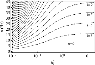
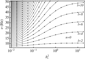
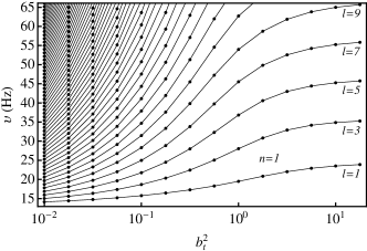
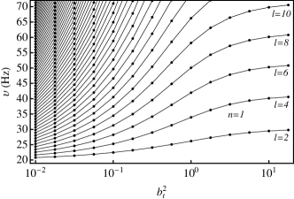
Figure 1: Splitting of the Alfvén continuum as a tangled field is added to a smooth field. We have fixed $(B_{d}^{2}+\langle B_{t}^{2}\rangle)^{1/2}=B_{d}(1+b_{t}^{2})^{1/2}$ to $10^{15}$ G to illustrate the smooth transition from the continuum to the isotropic tangle. For $l$ odd and $n=0$ (upper left panel), low-frequency modes exist that go to zero frequency for $b_{t}^{2}\rightarrow 0$; see equation (29).

The mode structure is shown in Figure 1 for constant total magnetic energy, with $(B_{d}^{2}+\langle B_{t}^{2}\rangle)^{1/2}$ fixed at $10^{15}$ G. Modes for which $u_{\phi}$ has even parity (odd $l$) and odd parity (even $l$) about $z=0$ have been plotted separately. For $b_{t}^{2}>>1$, the solutions to the isotropic problem (equation 23) are recovered. As $b_{t}^{2}$ is reduced, the modes become more closely spaced, approaching a continuum as $b_{t}^{2}\rightarrow 0$. In the limit $b_{t}^{2}\rightarrow 0$ the sequence of continua begins at $\sim 7(2n+1)$ Hz for odd-parity modes (even $l$) and $\sim 14n$ Hz for even-parity modes (odd $l$), in agreement with the continuum sequences described by equations (15) and (16). The $n=0$ odd modes approach zero as $b_{t}^{2}\rightarrow 0$ and scale as

$$\nu=6.70\,l\,b_{t}\,\left(\frac{z}{0.77}\right)\left(\frac{R}{10\mbox{ km}}\right)^{1/2}\left(\frac{M}{1.4M_{\odot}}\right)^{-1/2}\left(\frac{x_{p}}{0.1}\right)^{-1/2}\left(\frac{B_{d}}{10^{15}\mbox{ G}}\right)\,\mbox{ Hz}.$$ (29)

These modes approach rigid-body rotation solutions in the $b_{t}\rightarrow 0$ limit. Examination of the eigenmodes as $b_{t}^{2}\rightarrow 0$ also shows that the oscillation amplitude becomes sharply peaked at a specific value of the cylindrical radius $s$ and vanishes everywhere else, in agreement with the continuum solution in §2.

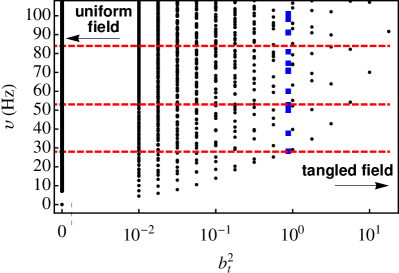
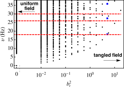
Figure 2: Splitting of the Alfvén continuum (the column on the far left of each figure) as a tangled field is added to a smooth field in SGR 1900 (left) and SGR 1806 (right). The dipole field strength $B_{d}$ is fixed to the value inferred from spin-down value: $7\times 10^{14}$ G for SGR 1900 and $2\times 10^{15}$ G for SGR 1806. Red-dashed lines correspond to observed QPO frequencies. Solid blue squares give the eigenfrequencies obtained from choosing the value of $b_{t}^{2}$ that matches the 28 Hz QPO in SGR 1900 and the 18 Hz QPO in SGR 1806. Not all detected QPOs are shown on the two scales. The lowest sequence of points approach the $k=0$ rigid-body mode, according to equation (29).

The splitting of the Alfvén continuum is shown in a different way in Figure 2, where predictions are made for the eigenfrequencies in SGR 1900 (left) and SGR 1806 (right). In contrast with Figure 1 where the total magnetic field was held constant ($(B_{d}^{2}+\langle B_{t}^{2}\rangle)^{1/2}=10^{15}$ G), we now fix $B_{d}$ in each magnetar to its observed dipole spin-down value: $7\times 10^{14}$ G for SGR 1900 and $2\times 10^{15}$ G for SGR 1806. We henceforth take the fiducial values of $M=1.4M_{\odot}$ and $R=10$ in each magnetar. Eigenfrequencies for all $n$ and $l$ for the range of frequencies shown are plotted. For $b_{t}^{2}=0$, there exists an Alfvén continuum that begins at $\simeq 7\,B^{d}_{15}$ Hz, with a zero-frequency solution corresponding to rigid-body rotation. As $b_{t}^{2}$ is increased, the continuum splits into discrete normal modes. As $b_{t}^{2}$ is further increased and the modes spread out further, the higher-frequency modes move off the diagram. For large $b_{t}^{2}$ the eigenfrequencies become large due to the large tangled field.

For fixed $M$ and $R$, the model has only $b_{t}^{2}$ as a free parameter. We tune $b_{t}^{2}$ to match the 28 Hz QPO observed in SGR 1900, arriving at $b_{t}^{2}=13.3$. Similarly, we tune $b_{t}^{2}$ to match the 18 Hz QPO observed in SGR 1806, arriving at $b_{t}^{2}=0.17$. Once $b_{t}^{2}$ is fixed in this way, we have quantitative predictions for the rest of the mode spectrum. Part of the mode spectrum is shown in Figure 2; the observed QPO frequencies are shown as horizontal red dashed lines, and the predicted eigenfrequencies as solid blue squares.

The predicted spectrum is given in more detail in Tables 1 and 2. In Table 1, we give the spectrum of eigenfrequencies predicted for SGR 1900. Fundamentals in boldface are within 3 Hz of an observed QPO, and denote plausible mode identifications. The predicted spectrum is about three times denser than the spectrum of observed QPOs. Overtones begin at higher frequencies, and cannot account for the observed QPO spectrum below 63 Hz. As we show in §3 of the accompanying Letter, overtones are more energetically costly than the fundamentals. We expect overtones to be more difficult to observe.

In Table 2, we give some of the eigenfrequencies predicted for SGR 1806. The spectrum is very dense, with a mode spacing of about 2 Hz if we adopt the inferred dipole field of $2\times 10^{15}$ G. If the dipole field has been overestimated, not implausible, then the predicted spectrum is much less dense, and more similar to SGR 1900. For example, taking $B_{d}$ equal to 0.62 of the reported value, a value of $b_{t}^{2}=1.0$ matches the 18 Hz QPO, and the predicted spectrum is that given in Table 3; the spectrum is less dense, with a spacing of about 7 Hz in the fundamentals.

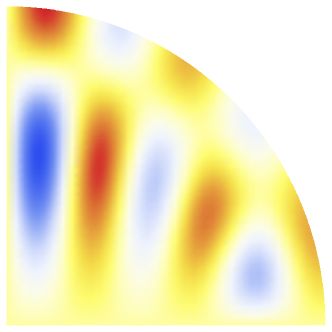
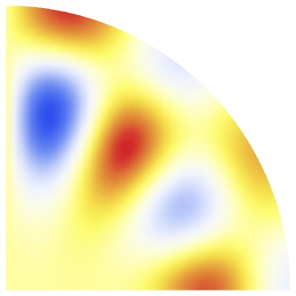
Figure 3: Example eigenmodes for SGR 1900 (left) and 1806 (right), see text for details. Light shading denotes motion out of the page for a given phase, and dark shading denotes motion into the page. The left panel corresponds to $b_{t}^{2}=13.3$ and exhibits the spherical structure of the isotropic limit, while the right corresponds to $b_{t}^{2}=0.17$ and exhibits the cylindrical structure of the continuum.

Examples of eigenmodes are plotted in Figure 3. The left panel shows the 82 Hz mode of SGR 1900, with the attribution $l=6$, $n=0$, while the right panel shows the 29 Hz mode of SGR 1806, with the attribution $l=5$, $n=0$. The left panel corresponds to $b_{t}^{2}=13.3$, which is close to the isotropic limit, and shows a large degree of spherical structure symmetry. In the plot on the right, $b_{t}^{2}=0.17$, and the mode shows mostly cylindrical structure, a characteristic feature of the continuum.

All examples shown here are for $R=10$ km and $M=1.4M_{\odot}$. The eigenfrequencies scale with the stellar compactness approximately as $(M/R)^{-1/2}$ for fixed $b_{t}^{2}$; see equation (23). If the compactness is increased, $b_{t}^{2}$ must also be increased to give the same spectrum.

5 Effects of density stratification and crust rigidity

We now show that the inclusion of density stratification and crust rigidity give small corrections to the eigenfrequencies obtained with the constant-density model for $b_{t}^{2}>>1$. For simplicity, we ignore the dipole field, and study the isotropic problem corresponding to a strong magnetic tangle. In these comparisons, we take the dipole field to have a strength of $B_{d}=7\times 10^{14}$ G, as measured for SGR 1900, and $b_{t}^{2}=13.3$ inferred above for this object.

We construct a relativistic star using the analytic representation of the Brussels-Montreal equation of state derived by Potekhin et al. (2013). For a 1.4 $M_{\odot}$ neutron star, we obtain a radius of 13.1 km. The shear modulus is from Strohmayer et al. (1991), and we fix $x_{p}=0.1$. For this spherical problem, the variable separation proceeds as in §3. We solve numerically for the radial eigenfunctions and eigenfrequencies. As a baseline for comparison, we use equation (23) to obtain the eigenfrequencies for a constant-density star of radius 13.1 km.

We assess the effects of density stratification by calculating the change in eigenfrequencies of a stratified star, without a rigid crust, relative to each eigenfrequency obtained from the constant-density model of radius $R=13.1$ km and of mass 1.4 $M_{\odot}$; see Table 4. The fundamental modes all shift up by about 20%. The overtones go down by about 15% or less, an effect that decreases with increasing $l$.

We assess the effects of crust rigidity by calculating the shift in eigenfrequencies of a stellar model with a crust relative to the same model with the material shear modulus set to zero. Crust rigidity increases the eigenfrequencies by about 4% or less for the fundamentals, and about 1% or less for overtones. These results are in quantitative agreement with the simple two-zone calculation of these effects presented in §4 of the accompanying Letter.

In summary, density stratification increases the frequencies of the fundamental modes by about 20% relative to the constant-density model, a shift that can be almost completely subsumed in the constant-density model with different choices of radius or mass. Overtones are shifted down by 15% or less, an effect that decreases with $l$. The effects of crust rigidity are small enough - less than 4% - that the crust can be ignored.

These conclusions hold for $b_{t}^{2}>>1$, as we have inferred for SGR 1900. For SGR 1806, with an inferred value of $b_{t}^{2}$ of $0.17$, the effects of the crust could be important, while we expect the effects of density stratification to be about the same.

Appendix A Variable Separation

Equations (25) and (26) can be separated and solved by transforming to an oblate spheroidal coordinate system $(u,v)$ defined by

$$s=R\sqrt{\frac{\left(1+b_{t}^{2}u^{2}\right)\left(1-v^{2}\right)}{1+b_{t}^{2}}}$$ (A1)

$$z=Ruv$$ (A2)

Curves of constant $u$ are ellipses, and curves of constant $v$ are hyperbolae. For $u=1$, the coordinate gives a sphere of radius $R$. In the limit $b_{t}^{2}\rightarrow\infty$, spherical coordinates are recovered with $u=r/R$ and $v=\cos\theta$.

In these coordinates, equation (25) becomes

$$\left(1+b_{t}^{2}u^{2}\right)\frac{\partial^{2}u_{\phi}}{\partial u^{2}}+ 2b_{t}^{2}u\frac{\partial u_{\phi}}{\partial u}+\frac{b_{t}^{2}u_{\phi}}{1+b_{t}^{2}u^{2}}+b_{t}^{2}\left(1-v^{2}\right)\frac{\partial^{2}u_{\phi}}{\partial v^{2}}$$

$$-2b_{t}^{2}v\frac{\partial u_{\phi}}{\partial v}-\frac{b_{t}^{2}u_{\phi}}{1-v^{2}}+\bar{\omega}^{2}\left(b_{t}^{2}u^{2}+v^{2}\right)u_{\phi}=0$$

where

$$\bar{\omega}\equiv\frac{R\omega}{c_{t}}\sqrt{\frac{b_{t}^{2}}{1+b_{t}^{2}}},$$ (A3)

and $c_{t}^{2}\equiv\langle B_{t}^{2}\rangle/(4\pi\rho_{d})$.

The boundary condition equation (26) at $u=1$ becomes

$$(1+b_{t}^{2})\frac{\partial u_{\phi}}{\partial u}-b_{t}^{2}u_{\phi}=0,$$ (A4)

while at $z=0$ we require

$$u_{\phi}=0\,,$$ (A5)

for odd parity modes, and

$$\left(1+b_{t}^{2}u^{2}\right)v\frac{\partial u_{\phi}}{\partial u}+b_{t}^{2}\left(1-v^{2}\right)u\frac{\partial u_{\phi}}{\partial v}=0\,,$$ (A6)

for even parity modes.

We seek a separable solution of the form

$$u_{\phi}(u,v)=U(u)V(v).$$ (A7)

Equation (A) becomes

$$\left(1+b_{t}^{2}u^{2}\right)\frac{d^{2}U}{du^{2}}+2b_{t}^{2}u\frac{dU}{du}+\frac{b_{t}^{2}U}{1+b_{t}^{2}u^{2}}-\kappa b_{t}^{2}U+\bar{\omega}^{2}b_{t}^{2}u^{2}U=0$$ (A8)

$$b_{t}^{2}\left(1-v^{2}\right)\frac{d^{2}V}{dv^{2}}-2b_{t}^{2}v\frac{dV}{dv}-\frac{b_{t}^{2}V}{1-v^{2}}+\kappa b_{t}^{2}V+\bar{\omega}^{2}v^{2}V=0,$$ (A9)

where $\kappa$ is the separation constant. The boundary condition eq. (A4) becomes

$$(1+b_{t}^{2})\frac{dU}{du}-b_{t}^{2}U=0,$$ (A10)

at $u=1$. The boundary conditions (A5) and (A6) are satisfied if we impose

$$U(0)=0\hskip 14.22636pt\mbox{and}\hskip 14.22636ptV(0)=0\,,$$ (A11)

for odd parity modes or

$$U^{\prime}(0)=0\hskip 14.22636pt\mbox{and}\hskip 14.22636ptV^{\prime}(0)=0\,,$$ (A12)

for even parity modes.

In the limit $b_{t}^{2}\rightarrow\infty$, equation (A8) reduces to the spherical Bessel equation with solution $U(u)=j(\bar{\omega}u)$, while (A9) reduces to an associated Legendre equation with solution $V(v)=\sqrt{1-v^{2}}\partial P^{0}_{l}/\partial v=-P^{1}_{l}(v)$ and $\kappa=l(l+1)$, which recovers the solutions of the isotropic model of §3.

We solve equations (A8), (A9), (A10) numerically for the normal mode frequencies. For arbitrary $b_{t}^{2}$ the modes are identified by the number of nodes; for the $n^{th}$ mode the function $U(u)$ has $n$ nodes on the domain $0\leq u\leq 1$, while for the $l^{th}$ mode the function $V(v)$ has $l-1$ nodes on $-1\leq v\leq 1$.

$l$	$n=0$	$n=1$	$n=2$	$n=3$
1	0	63	99	134
2	28	79	116	152
3	43	93	130
4	56	107	146
5	69	120	160
6	82	134
7	94	147
8	106
9	118
10	130
11	142
12	154

Table 1: Predicted eigenfrequencies in Hz for SGR 1900 with $B_{d}=7\times 10^{14}$ G and $b_{t}^{2}=13.3$. Fundamentals in boldface are within 3 Hz of an observed QPO, and denote plausible mode identifications. We do not list frequencies above 160 Hz.

$l$	$n=0$	$n=1$	$n=2$	$n=3$	$n=4$
1	0	35	65	93	122
2	20	50	79	108	135
3	18	44	72	101	130
4	28	58	87	115	143
5	29	52	80	109	137
6	38	66	95	123	151
7	40	62	89	117	145
8	48	75	102	131	159
9	51	71	97	125	153
10	58	84	111	139

Table 2: Some of the eigenfrequencies in Hz predicted for SGR 1806 assuming, $B_{d}=2\times 10^{15}$ G. The 18 Hz QPO requires $b_{t}^{2}=0.17$, giving a very dense spectrum.

$l$	$n=0$	$n=1$	$n=2$	$n=3$	$n=4$
1	0	34	58	81	104
2	18	46	70	93	116
3	25	49	72	94	117
4	32	59	82	106	129
5	39	65	85	107	130
6	46	74	96	119	142
7	53	80	100	121	143
8	60	88	110	132	155
9	66	95	115	135	157
10	73	102	124	146

Table 3: Some of the eigenfrequencies in Hz predicted for SGR 1806 assuming, $B_{d}=1.24\times 10^{15}$ G. The 18 Hz QPO requires $b_{t}^{2}=1.0$. Fundamentals in boldface are within 3 Hz of an observed QPO, and denote plausible mode identifications. We do not list frequencies above 160 Hz.

$l$	$n=0$	$n=1$	$n=2$	$n=3$
1	-	-15%	-15%	-15%
2	+21%	-12%	-14%	-15%
3	+21%	-9.8%	-13%
4	+21%	-7.8%	-12%
5	+21%	-6.1%	-10%
6	+20%	-4.8%	-10%
7	+20%	-3.7%
8		-2.7%

Table 4: Percentage frequency change of modes in a stratified star with no crust shear modulus compared with a constant density star with the same mass and radius. We use a 1.4 $M_{\odot}$ star with radius 13.1 km, taking $x_{p}=0.1$, $B_{d}=7\times 10^{14}$ G, and $b_{t}^{2}=13.3$.

$l$	$n=0$	$n=1$	$n=2$	$n=3$
1	-	0.0 %	0.0%	0.0%
2	+4.3%	0.61%	0.36%	0.17%
3	+4.1%	0.93%	0.57%
4	+3.4%	1.2%	0.76%
5	+2.8%	1.5%	0.86%
6	+2.2%	1.6%	1.2%
7	+1.8%

Table 5: Percentage frequency change of modes in a stratified star with a crust compared with a stratified star with no crust shear modulus, for the parameters of Table 4.

References

- Barat et al. (1979) Barat, C., Chambon, G., Hurley, K., Niel, M., Vedrenne, G., Estulin, I., Kurt, V., & Zenchenko, V. 1979, Astronomy and Astrophysics, 79, L24
- Braithwaite (2008) Braithwaite, J. 2008, Monthly Notices of the Royal Astronomical Society, 386, 1947
- Braithwaite (2009) —. 2009, Mon. Not. Roy. Astron. Soc., 397, 763
- Braithwaite & Nordlund (2006) Braithwaite, J. & Nordlund, Å. 2006, Astronomy & Astrophysics, 450, 1077
- Braithwaite & Spruit (2006) Braithwaite, J. & Spruit, H. 2006, Astronomy & Astrophysics, 450, 1097
- Brandenburg & Subramanian (2005) Brandenburg, A. & Subramanian, K. 2005, Physics Reports, 417, 1
- Cerdá-Durán et al. (2009) Cerdá-Durán, P., Stergioulas, N., & Font, J. A. 2009, Mon. Not. Roy. Astron. Soc., 397, 1607
- Cerdá-Durán et al. (2009) Cerdá-Durán, P., Stergioulas, N., & Font, J. A. 2009, Monthly Notices of the Royal Astronomical Society, 397, 1607
- Chamel (2005) Chamel, N. 2005, Nucl. Phys. A, 747, 109
- Chamel (2012) —. 2012, Phys. Rev. C, 85, 035801
- Chamel & Haensel (2006) Chamel, N. & Haensel, P. 2006, Phys. Rev. C, 73, 045802
- Cline et al. (1980) Cline, T., Desai, U., Pizzichini, G., Teegarden, B., Evans, W., Klebesadel, R., Laros, J., Hurley, K., Niel, M., & Vedrenne, G. 1980, The Astrophysical Journal, 237, L1
- Colaiuda et al. (2009) Colaiuda, A., Beyer, H., & Kokkotas, K. 2009, Monthly Notices of the Royal Astronomical Society, 396, 1441
- Colaiuda & Kokkotas (2011) Colaiuda, A. & Kokkotas, K. D. 2011, Mon. Not. Roy. Astron. Soc., 414, 3014
- D’Angelo & Watts (2012) D’Angelo, C. & Watts, A. 2012, The Astrophysical Journal Letters, 751, L41
- Douchin & Haensel (2001) Douchin, F. & Haensel, P. 2001, Astron. Astrophys., 380, 151
- El-Mezeini & Ibrahim (2010) El-Mezeini, A. M. & Ibrahim, A. I. 2010, Astrophys. J. Lett., 721, L121
- Esposito et al. (2010) Esposito, P., Israel, G. L., Turolla, R., Tiengo, A., Götz, D., de Luca, A., Mignani, R. P., Zane, S., Rea, N., Testa, V., Caraveo, P. A., Chaty, S., Mattana, F., Mereghetti, S., Pellizzoni, A., & Romano, P. 2010, MNRAS, 405, 1787
- Fenimore et al. (1996) Fenimore, E. E., Klebesadel, R. W., & Laros, J. G. 1996, Astrophys. J., 460, 964
- Feroci et al. (1999) Feroci, M., Frontera, F., Costa, E., Amati, L., Tavani, M., Rapisarda, M., & Orlandini, M. 1999, The Astrophysical Journal Letters, 515, L9
- Flowers & Ruderman (1977) Flowers, E. & Ruderman, M. 1977, The Astrophysical Journal, 215, 302
- Gabler et al. (2011) Gabler, M., Cerdá-Durán, P., Font, J. A., Müller, E., & Stergioulas, N. 2011, Mon. Not. Roy. Astron. Soc., 410, L37
- Gabler et al. (2013a) Gabler, M., Cerdá-Durán, P., Font, J. A., Müller, E., & Stergioulas, N. 2013a, Monthly Notices of the Royal Astronomical Society, 430, 1811
- Gabler et al. (2012) Gabler, M., Cerdá-Durán, P., Stergioulas, N., Font, J. A., & Müller, E. 2012, Monthly Notices of the Royal Astronomical Society, 421, 2054
- Gabler et al. (2013b) —. 2013b, Physical review letters, 111, 211102
- Gabler et al. (2014) —. 2014, Monthly Notices of the Royal Astronomical Society, 443, 1416
- Glampedakis et al. (2006) Glampedakis, K., Samuelsson, L., & Andersson, N. 2006, Mon. Not. Roy. Astron. Soc., 371, L74
- Goedbleod & Poedts (2004) Goedbleod, J. P. H. & Poedts, S. 2004, Principles of Magnetohydrodynamics (Cambridge Univ. Press, Cambridge)
- Haensel & Potekhin (2004) Haensel, P. & Potekhin, A. Y. 2004, Astron. Astrophys., 428, 191
- Hambaryan et al. (2011) Hambaryan, V., Neuhäuser, R., & Kokkotas, K. D. 2011, Astron. Astrophys., 528, 45
- Huppenkothen et al. (2014a) Huppenkothen, D., D’Angelo, C., Watts, A. L., Heil, L., van der Klis, M., van der Horst, A. J., Kouveliotou, C., Baring, M. G., Göğüş, E., Granot, J., et al. 2014a, The Astrophysical Journal, 787, 128
- Huppenkothen et al. (2014b) Huppenkothen, D., Heil, L., Watts, A., & Göğüş, E. 2014b, The Astrophysical Journal, 795, 114
- Huppenkothen et al. (2013) Huppenkothen, D., Watts, A. L., Uttley, P., van der Horst, A. J., van der Klis, M., Kouveliotou, C., Göğüş, E., Granot, J., Vaughan, S., & Finger, M. H. 2013, The Astrophysical Journal, 768, 87
- Hurley et al. (1999) Hurley, K., Cline, T., Mazets, E., Barthelmy, S., Butterworth, P., Marshall, F., Palmer, D., Aptekar, R., Golenetskii, S., Il’Inskii, V., et al. 1999, Nature, 397, 41
- Israel et al. (2005) Israel, G., Belloni, T., Stella, L., Rephaeli, Y., Gruber, D., Casella, P., Dall’Osso, S., Rea, N., Persic, M., & Rothschild, R. 2005, The Astrophysical Journal Letters, 628, L53
- Levin (2006) Levin, Y. 2006, Mon. Not. Roy. Astron. Soc., 368, L35
- Levin (2007) —. 2007, Mon. Not. Roy. Astron. Soc., 377, 159
- Link & van Eysden (2015) Link, B. & van Eysden, C. A. 2015, arXiv:1503.01410
- Link & van Eysden (2016) —. 2016, ApJ, in press, (Supplementary materials)
- Mazets et al. (1979) Mazets, E., Golenetskii, S., Il’Inskii, V., Aptekar, R., & Guryan, Y. A. 1979, Nature, 282, 587
- Mereghetti et al. (2006) Mereghetti, S., Esposito, P., Tiengo, A., Zane, S., Turolla, R., Stella, L., Israel, G., Götz, D., & Feroci, M. 2006, The Astrophysical Journal, 653, 1423
- Nakagawa et al. (2008) Nakagawa, Y. E., Mihara, T., Yoshida, A., Yamaoka, K., Sugita, S., Murakami, T., Yonetoku, D., Suzuki, M., Nakajima, M., Tashiro, M., et al. 2008, PASJ, 61, S387
- Passamonti & Lander (2013) Passamonti, A. & Lander, S. 2013, Monthly Notices of the Royal Astronomical Society, 429, 767
- Rea et al. (2010) Rea, N., Esposito, P., Turolla, R., Israel, G. L., Zane, S., Stella, L., Mereghetti, S., Tiengo, A., Götz, D., Göğüş, E., & Kouveliotou, C. 2010, Science, 330, 944
- Rea et al. (2012) Rea, N., Israel, G. L., Esposito, P., Pons, J. A., Camero-Arranz, A., Mignani, R. P., Turolla, R., Zane, S., Burgay, M., Possenti, A., Campana, S., Enoto, T., Gehrels, N., Göǧüş, E., Götz, D., Kouveliotou, C., Makishima, K., Mereghetti, S., Oates, S. R., Palmer, D. M., Perna, R., Stella, L., & Tiengo, A. 2012, ApJ, 754, 27
- Rea et al. (2014) Rea, N., Viganò, D., Israel, G. L., Pons, J. A., & Torres, D. F. 2014, ApJ, 781, L17
- Sotani (2015) Sotani, H. 2015, Phys. Rev. D, 92, 104024
- Sotani et al. (2008a) Sotani, H., Colaiuda, A., & Kokkotas, K. D. 2008a, Mon. Not. Roy. Astron. Soc., 385, 2162
- Sotani et al. (2008b) Sotani, H., Kokkotas, K. D., & Stergioulas, N. 2008b, Mon. Not. Roy. Astron. Soc., 385, L5
- Strohmayer et al. (1991) Strohmayer, T. E., van Horn, H. M., Ogata, S., Iyetomi, H., & Ichimaru, S. 1991, Astrophys. J., 375, 679
- Strohmayer & Watts (2005) Strohmayer, T. E. & Watts, A. L. 2005, Astrophys. J., 632, L111
- Strohmayer & Watts (2006) —. 2006, The Astrophysical Journal, 653, 593
- Tayler (1973) Tayler, R. 1973, Monthly Notices of the Royal Astronomical Society, 161, 365
- Thompson & Duncan (1993) Thompson, C. & Duncan, R. C. 1993, Astrophys. J., 408
- Tiengo et al. (2009) Tiengo, A., Esposito, P., Mereghetti, S., Israel, G., Stella, L., Turolla, R., Zane, S., Rea, N., Götz, D., & Feroci, M. 2009, Mon. Not. Roy. Astron. Soc., 399, L74
- Timokhin et al. (2008) Timokhin, A., Eichler, D., & Lyubarsky, Y. 2008, The Astrophysical Journal, 680, 1398
- Turolla et al. (2011) Turolla, R., Zane, S., Pons, J., Esposito, P., & Rea, N. 2011, The Astrophysical Journal, 740, 105
- van der Horst et al. (2010) van der Horst, A. J., Connaughton, V., Kouveliotou, C., Göǧüş, E., Kaneko, Y., Wachter, S., Briggs, M. S., Granot, J., Ramirez-Ruiz, E., Woods, P. M., Aptekar, R. L., Barthelmy, S. D., Cummings, J. R., Finger, M. H., Frederiks, D. D., Gehrels, N., Gelino, C. R., Gelino, D. M., Golenetskii, S., Hurley, K., Krimm, H. A., Mazets, E. P., McEnery, J. E., Meegan, C. A., Oleynik, P. P., Palmer, D. M., Pal’shin, V. D., Pe’er, A., Svinkin, D., Ulanov, M. V., van der Klis, M., von Kienlin, A., Watts, A. L., & Wilson-Hodge, C. A. 2010, ApJ, 711, L1
- van Hoven & Levin (2011) van Hoven, M. & Levin, Y. 2011, Mon. Not. Roy. Astron. Soc., 420, 1036
- van Hoven & Levin (2012) —. 2012, Monthly Notices of the Royal Astronomical Society, 420, 3035
- Watts & Strohmayer (2006) Watts, A. L. & Strohmayer, T. E. 2006, Astrophys. J., 637, L117
- Wright (1973) Wright, G. A. E. 1973, Mon. Not. Roy. Astron. Soc., 162, 339

References

- Chamel & Haensel (2006) Chamel, N. & Haensel, P. 2006, Phys. Rev. C, 73, 045802
- Levin (2007) Levin, Y. 2007, Mon. Not. Roy. Astron. Soc., 377, 159
- Potekhin et al. (2013) Potekhin, A., Fantina, A., Chamel, N., Pearson, J., & Goriely, S. 2013, Astronomy & astrophysics, 560, A48
- Strohmayer et al. (1991) Strohmayer, T. E., van Horn, H. M., Ogata, S., Iyetomi, H., & Ichimaru, S. 1991, Astrophys. J., 375, 679