The decays $h^{0}\to b\bar{b}$ and $h^{0}\to c\bar{c}$ in the light of the MSSM with quark flavour violation

Abstract

We calculate the decay width of $h^{0}\to b\bar{b}$ in the Minimal Supersymmetric Standard Model (MSSM) with quark flavour violation (QFV) at full one-loop level. We study the effect of $\tilde{c}-\tilde{t}$ mixing and $\tilde{s}-\tilde{b}$ mixing taking into account the constraints from the B meson data. We discuss and compare in detail the decays $h^{0}\to c\bar{c}$ and $h^{0}\to b\bar{b}$ within the framework of the perturbative mass insertion technique using the Flavour Expansion Theorem. The deviation of both decay widths from the Standard Model values can be quite large. Whereas in $h^{0}\to c\bar{c}$ it is almost entirely due to the flavour violating part of the MSSM, in $h^{0}\to b\bar{b}$ it is mainly due to the flavour conserving part. Nevertheless, the QFV contribution to $\Gamma(h^{0}\to b\bar{b})$ due to $\tilde{c}-\tilde{t}$ mixing and chargino exchange can go up to $\sim 7\%$.

1 Introduction

In the Standard Model (SM) the Higgs mechanism is responsible for the mass of the fermions. Therefore, it is necessary to measure the Yukawa couplings very precisely. Since the Yukawa coupling is proportional to the fermion mass, the largest decay branching ratio of the Higgs boson, discovered by CMS and ATLAS at LHC Aad:2012tfa ; Chatrchyan:2012xdj with a mass of approximately 125 GeV, is that of $h^{0}\to b\bar{b}$. Within the SM this branching ratio is B$(h^{0}\to b\bar{b})=0.577~{}^{\tiny{+3.2\%}}_{\tiny{-3.3\%}}$ pdg2014 . Although the Higgs boson properties measured so far are consistent with the SM, deviations from the SM are not yet excluded and could point to "New Physics".

An important extension of the SM is provided by Supersymmetry (SUSY), in particular by the Minimal Supersymmetric Standard Model (MSSM). In the MSSM, the discovered Higgs boson could be the lightest neutral Higgs boson $h^{0}$. Quark flavour conservation (QFC) is usually assumed (apart from the quark flavour violation (QFV) induced by the Cabibbo-Kobayashi-Maskawa (CKM) matrix). However, SUSY QFV terms could be present in the mass mixing matrix of the squarks, especially mixing terms between the 2nd and the 3rd squark generations.

In a previous paper Bartl:2014bka we studied the impact of $\tilde{c}_{L,R}-\tilde{t}_{L,R}$ mixing on the decay $h^{0}\to c\bar{c}$. We showed that the deviation from the SM width $\Gamma(h^{0}\to c\bar{c})$ can go up to $\pm 35\%$, due to QFV effects at one-loop level. In the present paper, we study the influence of this mixing in the decay $h^{0}\to b\bar{b}$. (For completeness we have also studied $\tilde{s}_{L,R}-\tilde{b}_{L,R}$ mixing effects, but they have turned out to be very small.) There are, however, constraints on the mixing between the $2^{\rm nd}$ and the $3^{\rm rd}$ generations of squarks from B-physics measurements ($\Delta M_{B_{s}},~{}{\rm B}(b\to s\gamma),~{}{\rm B}(b\to sl^{+}l^{-}),~{}{\rm B}(B_{s}\to\mu^{+}\mu^{-}),~{}{\rm B}(B^{+}\to\tau^{+}\nu)$), as well as from $m_{h^{0}}$ measurements and SUSY particle searches. We take into account all these constraints.

First, in our calculation of $\Gamma(h^{0}\to b\bar{b})$ at full one-loop level, we will largely proceed analogously to the case of $h^{0}\to c\bar{c}$ Bartl:2014bka ; Eberl:2014dla ; Hidaka:2015zqa ; Ginina:2015doa ; Hidaka:2015ewt , except for the particular features characteristic of the decays into bottom quarks, as the large $\tan\beta$ enhancement and resummation of the bottom Yukawa coupling.

The main new feature in this paper is the additional adoption of the perturbative mass insertion technique using the Flavour Expansion Theorem Dedes:2015twa . We will discuss it both in the $h^{0}\to c\bar{c}$ and $h^{0}\to b\bar{b}$ case. It gives systematic insight into the various QFV contributions. In particular, we show that due to the fact that the product $T^{U}_{32}M^{U}_{23}$ is apriori unbounded by experiment, the correction to the width of $h^{0}\to c\bar{c}$ can become large so that perturbation theory breaks down. (For the definitions of $T^{U}$ and $M^{U}$ see eqs. (1), (2) and (23) below.) In the $h^{0}\to b\bar{b}$ case this is not possible.

2 Definition of the QFV parameters

In the MSSM’s super-CKM basis of $\tilde{q}_{0\gamma}=(\tilde{q}_{1{\rm L}},\tilde{q}_{2{\rm L}},\tilde{q}_{3{\rm L}}$, $\tilde{q}_{1{\rm R}},\tilde{q}_{2{\rm R}},\tilde{q}_{3{\rm R}}),~{}\gamma=1,...6,$ with $(q_{1},q_{2},q_{3})=(u,c,t),$ $(d,s,b)$, one can write the squark mass matrices in their most general $3\times 3$-block form Allanach:2008qq

$${\cal M}^{2}_{\tilde{q}}=\left(\begin{array}[]{cc}{\cal M}^{2}_{\tilde{q},LL}&{\cal M}^{2}_{\tilde{q},LR}\\[5.69054pt] {\cal M}^{2}_{\tilde{q},RL}&{\cal M}^{2}_{\tilde{q},RR}\end{array}\right),$$ (1)

with $\tilde{q}=\tilde{u},\tilde{d}$. The left-left and right-right blocks in eq. (1) are given by

$${\cal M}^{2}_{\tilde{u},LL}=V_{\rm CKM}M_{Q}^{2}V_{\rm CKM}^{{\dagger}}+D_{\tilde{u},LL}{\bf 1}+\hat{m}^{2}_{u},$$

$${\cal M}^{2}_{\tilde{u},RR}=M_{U}^{2}+D_{\tilde{u},RR}{\bf 1}+\hat{m}^{2}_{u},$$

$${\cal M}^{2}_{\tilde{d},LL}=M_{Q}^{2}+D_{\tilde{d},LL}{\bf 1}+\hat{m}^{2}_{d},$$

$${\cal M}^{2}_{\tilde{d},RR}=M_{D}^{2}+D_{\tilde{d},RR}{\bf 1}+\hat{m}^{2}_{d},$$ (2)

where $M_{Q,U,D}$ are the hermitian soft SUSY-breaking mass matrices of the squarks and $\hat{m}_{u,d}$ are the diagonal mass matrices of the up-type and down-type quarks. Furthermore, $D_{\tilde{q},LL}=\cos 2\beta m_{Z}^{2}(T_{3}^{q}-e_{q}\sin^{2}\theta_{W})$ and $D_{\tilde{q},RR}=e_{q}\sin^{2}\theta_{W}\times$ $\cos 2\beta m_{Z}^{2}$, where $T_{3}^{q}$ and $e_{q}$ are the isospin and electric charge of the quarks (squarks), respectively, and $\theta_{W}$ is the weak mixing angle. Due to the $SU(2)_{\rm L}$ symmetry the left-left blocks of the up-type and down-type squarks in eq. (2) are related by the CKM matrix $V_{\rm CKM}$. The left-right and right-left blocks of eq. (1) are given by

$${\cal M}^{2}_{\tilde{u},RL}={\cal M}^{2{\dagger}}_{\tilde{u},LR} = \frac{v_{2}}{\sqrt{2}}T_{U}-\mu^{*}\hat{m}_{u}\cot\beta,$$

$${\cal M}^{2}_{\tilde{d},RL}={\cal M}^{2{\dagger}}_{\tilde{d},LR} = \frac{v_{1}}{\sqrt{2}}T_{D}-\mu^{*}\hat{m}_{d}\tan\beta,$$ (3)

where $T_{U,D}$ are the soft SUSY-breaking trilinear coupling matrices of the up-type and down-type squarks entering the Lagrangian ${\cal L}_{int}\supset-(T_{U\alpha\beta}\tilde{u}^{\dagger}_{R\alpha}\tilde{u}_{L\beta}H^{0}_{2}$ $+T_{D\alpha\beta}\tilde{d}^{\dagger}_{R\alpha}\tilde{d}_{L\beta}H^{0}_{1})$, $\mu$ is the higgsino mass parameter, and $\tan\beta$ is the ratio of the vacuum expectation values of the neutral Higgs fields $v_{2}/v_{1}$, with $v_{1,2}=\sqrt{2}\left\langle H^{0}_{1,2}\right\rangle$. The squark mass matrices are diagonalized by the $6\times 6$ unitary matrices $U^{\tilde{q}}$, $\tilde{q}=\tilde{u},\tilde{d}$, such that

$$U^{\tilde{q}}{\cal M}^{2}_{\tilde{q}}(U^{\tilde{q}})^{{\dagger}}={\rm diag}(m_{\tilde{q}_{1}}^{2},\dots,m_{\tilde{q}_{6}}^{2})\,,$$ (4)

with $m_{\tilde{q}_{1}}<\dots<m_{\tilde{q}_{6}}$. The physical mass eigenstates $\tilde{q}_{i},i=1,...,6$ are given by $\tilde{q}_{i}=U^{\tilde{q}}_{i\alpha}\tilde{q}_{0\alpha}$.

We define the QFV parameters in the up-type squark sector $\delta^{LL}_{\alpha\beta}$, $\delta^{uRR}_{\alpha\beta}$ and $\delta^{uRL}_{\alpha\beta}$ $(\alpha\neq\beta)$ as follows Gabbiani:1996hi :

$$\delta^{LL}_{\alpha\beta} \equiv M^{2}_{Q\alpha\beta}/\sqrt{M^{2}_{Q\alpha\alpha}M^{2}_{Q\beta\beta}}~{},$$ (5)

$$\delta^{uRR}_{\alpha\beta} \equiv M^{2}_{U\alpha\beta}/\sqrt{M^{2}_{U\alpha\alpha}M^{2}_{U\beta\beta}}~{},$$ (6)

$$\delta^{uRL}_{\alpha\beta} \equiv (v_{2}/\sqrt{2})T_{U\alpha\beta}/\sqrt{M^{2}_{U\alpha\alpha}M^{2}_{Q\beta\beta}}~{},$$ (7)

where $\alpha,\beta=1,2,3~{}(\alpha\neq\beta)$ denote the quark flavours $u,c,t$. Analogously, for the down-type squark sector we have

$$\delta^{dRR}_{\alpha\beta} \equiv M^{2}_{D\alpha\beta}/\sqrt{M^{2}_{D\alpha\alpha}M^{2}_{D\beta\beta}}~{},$$ (8)

$$\delta^{dRL}_{\alpha\beta} \equiv (v_{1}/\sqrt{2})T_{D\alpha\beta}/\sqrt{M^{2}_{D\alpha\alpha}M^{2}_{Q\beta\beta}}~{},$$ (9)

and the parameter $\delta^{LL}_{\alpha\beta}$ is defined by eq.(5). The subscripts $\alpha,\beta=1,2,3~{}(\alpha\neq\beta)$ denote the quark flavours $d,s,b$.

In this paper we focus on the $\tilde{c}_{R}-\tilde{t}_{L}$, $\tilde{c}_{L}-\tilde{t}_{R}$, $\tilde{c}_{R}-\tilde{t}_{R}$, and $\tilde{c}_{L}-\tilde{t}_{L}$ mixing which is described by the QFV parameters $\delta^{uRL}_{23}$, $\delta^{uLR}_{23}\equiv(\delta^{uRL}_{32})^{*}$, $\delta^{uRR}_{23}$, and $\delta^{LL}_{23}$, respectively. The $\tilde{t}_{R}-\tilde{t}_{L}$ mixing is described by the QFC parameter $\delta^{uRL}_{33}$. We also allow $\tilde{s}-\tilde{b}$ mixing. All parameters are assumed to be real, i.e. no CP-violation is considered. In principle, there might be in addition also trilinear non-holomorphic interactions, see eq. (1.5) in Dedes:2014asa . These interactions are not taken into account in this study.

3 $h^{0}\to b\bar{b}$ at one-loop level with flavour violation

We write the decay width of $h^{0}\to b\bar{b}$ including the one-loop contributions as

$$\Gamma(h^{0}\to b\bar{b})=\Gamma^{\rm tree}(h^{0}\to b\bar{b})+\delta\Gamma^{\rm 1loop}(h^{0}\to b\bar{b})$$ (10)

with the tree-level decay width

$$\Gamma^{\rm tree}(h^{0}\to b\bar{b})=\frac{\rm N_{C}}{8\pi}m_{h^{0}}(s_{1}^{b})^{2}\bigg{(}1-\frac{4m_{b}^{2}}{m_{h^{0}}^{2}}\bigg{)}^{3/2}\,,$$ (11)

where ${N_{C}}=3$, $m_{h^{0}}$ is the on-shell mass of $h^{0}$ and the tree-level coupling $s_{1}^{b}$ is

$$s_{1}^{b}=g\frac{m_{b}}{2m_{W}}\frac{\sin{\alpha}}{\cos{\beta}}=\frac{h_{b}}{\sqrt{2}}\sin{\alpha}\,,$$ (12)

$\alpha$ is the mixing angle of the two CP-even Higgs bosons, $h^{0}$ and $H^{0}$ G&H .

In the calculation of $\delta\Gamma^{\rm 1loop}(h^{0}\to b\bar{b})$ we proceed in a way analogously to the calculation of $\delta\Gamma^{\rm 1loop}(h^{0}\to c\bar{c})$ in Ref. Bartl:2014bka . In addition to the diagrams that contribute within the SM, $\delta\Gamma^{\rm 1loop}(h^{0}\to b\bar{b})$ receives contributions from the exchange of SUSY particles and Higgs bosons. The corresponding diagrams are shown in Fig. 2 of Bartl:2014bka , replacing $c$ by $b$ quarks and $\tilde{u}\leftrightarrow\tilde{d}$. The dominant SUSY contribution is due to gluino and chargino exchange. The gluino and the chargino contribute also to the self-energy of the b quark.

As in Ref. Bartl:2014bka we use the ${\overline{\rm DR}}$ renormalisation scheme, where all input parameters in the Lagrangian (masses, fields and coupling parameters) are UV finite, defined at the scale $Q=1~{}\rm TeV$. In order to obtain the shifts from the ${\overline{\rm DR}}$ masses and fields to the physical scale-independent quantities, we use on-shell renormalisation conditions. Moreover, we include in our calculations the contributions from real hard gluon/photon radiation from the final b quarks.

The one-loop corrected width $\Gamma(h^{0}\to b\bar{b})$ is therefore given by

$$\Gamma(h^{0}\to b\bar{b})=\Gamma^{g,\rm impr}+\delta\Gamma^{\tilde{g}}+\delta\Gamma^{EW}\,,$$ (13)

where $\Gamma^{g,\rm impr}$ includes the tree-level and the gluon loop contribution, see eq.(55) in Bartl:2014bka , $\delta\Gamma^{\tilde{g}}$ is the gluino one-loop contribution and $\delta\Gamma^{EW}$ is the electroweak one-loop contribution. Moreover, we have considered the large $\tan\beta$ enhancement and the resummation of the bottom Yukawa coupling Carena:1999py . It turns out, however, that in our case with large $m_{A^{0}}$ close to the decoupling limit, the resummation effect is very small ($<0.1\%$).

4 Mass Insertion technique

In this section, we want to apply to the decays $h^{0}\to c\bar{c}$ and $h^{0}\to b\bar{b}$ the mass insertion technique as well as the Flavour Expansion Theorem (FET) as developed by Dedes et al. in Dedes:2015twa . Let us consider the expression

$$X=U^{\tilde{q}}_{iA}U^{\tilde{q}*}_{iB}B_{0}(0,m^{2},m^{2}_{\tilde{q}_{i}})\,,$$ (14)

with $A\neq B$. $U^{\tilde{q}}$ are defined with eq. (4) and $B_{0}$ are the two-point Passarino-Veltman functions. $X$ given in terms of mass eigenstates can be expanded into mass insertions (MIs) by the FET Dedes:2015twa

$$X = M^{I}_{AB}\,b_{0}\!\left(1,m^{2},\{M_{AA},M_{BB}\}\right)$$ (15)

$$+ M^{I}_{Ai}M^{I}_{iB}\,b_{0}\!\left(2,m^{2},\{M_{AA},M_{ii},M_{BB}\}\right)$$

$$+ M^{I}_{Ai}M^{I}_{ij}M^{I}_{jB}\,b_{0}\!\left(3,m^{2},\{M_{AA},M_{ii},M_{jj},M_{BB}\}\right)$$

$$+ M^{I}_{Ai}M^{I}_{ij}M^{I}_{jk}M^{I}_{kB}\,b_{0}\!\left(4,m^{2},\{M_{AA},M_{ii},M_{jj},M_{kk},M_{BB}\}\right)+\ldots\,,$$

by using Einstein summation convention. The diagonal elements of the squared mass matrix are denoted by $M_{ii}$, and the off-diagonal ones by the matrix $M^{I}$ with the restriction $M^{I}_{ii}=0$. This formula and all following MI formulas in this section have been checked with the Mathematica package MassToMI arXiv:1509.05030 . The generalized $b_{0}$ functions Dedes:2015twa , where the first argument shows how many insertions are done, can be written recursively as

$$b_{0}(1,a,\{b,c\}) = \frac{b_{0}(a,b)-b_{0}(a,c)}{b-c}\,,$$

$$b_{0}(2,a,\{b,c,d\}) = \frac{b_{0}(1,a,\{b,c\})-b_{0}(1,a,\{b,d\})}{c-d}\,,$$

$$b_{0}(3,a,\{b,c,d,e\}) = \frac{b_{0}(2,a,\{b,c,d\})-b_{0}(2,a,\{b,c,e\})}{d-e}\,,$$

$$b_{0}(4,a,\{b,c,d,e,f\}) = \frac{b_{0}(3,a,\{b,c,d,e\})-b_{0}(3,a,\{b,c,d,f\})}{e-f}\,,$$ (16)

with

$$b_{0}(a,b)\equiv B_{0}(0,a,b)=\frac{b\log\left(\frac{b}{Q^{2}}\right)-a\log\left(\frac{a}{Q^{2}}\right)}{a-b}+\Delta+1\,,$$ (17)

with the renormalisation scale $Q$ and $\Delta$ denotes the UV-divergence parameter. These functions are totally symmetric under any permutation of the set of arguments in the curly brackets. Note that $b_{0}(1,a,\{b,c\})\equiv c_{0}(a,b,c)\equiv C_{0}(0,0,0,a,b,c)$, $b_{0}(2,a,\{b,c,d\})\equiv D_{0}(0,0,0,0,0,0,a,b,c,d)$, etc., where $C_{0}$ and $D_{0}$ are the scalar 3-point and 4-point Passarino-Veltman functions PV . The general formula for a number of degenerate arguments is useful Dedes:2015twa ,

$$\lim_{\{x_{0},\ldots,x_{m}\}\to\{\xi,\ldots,\xi\}}b_{0}\!\left(k,a,\{x_{0},\ldots,x_{k}\}\right)={1\over m!}{\partial^{m}\over\partial\xi^{m}}b_{0}\!\left(k-m,a,\{\xi,x_{m+1},\ldots,x_{k}\}\right)\,,$$ (18)

for $k\geq 1$ and $m\leq k$. The derivative of $b_{0}$ with respect to the second argument reads

$$b_{0}{}^{(0,1)}(a,b)=\frac{1}{a-b}+\frac{a\log\left(\frac{b}{a}\right)}{(a-b)^{2}}\,.$$ (19)

The derivative of $b_{0}$ with respect to the first argument can be written as

$$b_{0}{}^{(1,0)}(a,b)=b_{0}{}^{(0,1)}(b,a)\,.$$ (20)

By using eq. (18) we can write $b_{0}(1,a,\{b,b\})$ as $b_{0}{}^{(0,1)}(a,b)$.

4.1 Gluino contribution to $h^{0}\to c\bar{c}$

As a first example, we want to calculate the self-energy of the c-quark due to $\tilde{g}$ and $\tilde{u}_{i}$ in the loop. We decompose the charm self-energy $\Sigma_{c}$ defined by the Lagrangian ${\cal L}=-\bar{c}\,\Sigma_{c}\,c$,

$$\Sigma_{c}(p)=\not{p}\left(\Sigma^{LL}_{c}(p^{2})P_{L}+\Sigma^{RR}_{c}(p^{2})P_{R}\right)+m_{c}\left(\Sigma^{RL}_{c}(p^{2})P_{L}+\Sigma^{LR}_{c}(p^{2})P_{R}\right)\,,$$ (21)

with $\Sigma^{LR}_{c}=\Sigma^{RL*}_{c}$. We assume real input parameters, therefore $\Sigma^{LR}_{c}=\Sigma^{RL}_{c}$, and

$$\Sigma^{LR,\tilde{g}}_{c}=-\frac{2\alpha_{s}}{3\pi}\frac{m_{\tilde{g}}}{m_{c}}\sum_{i=1}^{6}U^{\tilde{u}*}_{i2}U^{\tilde{u}}_{i5}B_{0}(m_{c}^{2},m^{2}_{\tilde{g}},m^{2}_{\tilde{u}_{i}})\,.$$ (22)

Allowing the squared $\tilde{u}$-mass matrix (eq. (1)) in the form

$${\cal M}^{2}_{\tilde{u}}=\left(\begin{array}[]{cc}{\cal M}^{2}_{\tilde{u},LL}&{\cal M}^{2}_{\tilde{u},LR}\\[5.69054pt] {\cal M}^{2}_{\tilde{u},RL}&{\cal M}^{2}_{\tilde{u},RR}\end{array}\right)\equiv M_{ij}=\left(\begin{array}[]{cccccc}M^{LL}_{11}&0&0&0&0&0\\ 0&M^{LL}_{22}&M^{Q}_{23}&0&0&\hat{v}_{2}T^{U}_{32}\\ 0&M^{Q}_{23}&M^{LL}_{33}&0&\hat{v}_{2}T^{U}_{23}&\hat{v}_{2}T^{U}_{33}\\ 0&0&0&M^{RR}_{11}&0&0\\ 0&0&\hat{v}_{2}T^{U}_{23}&0&M^{RR}_{22}&M^{U}_{23}\\ 0&\hat{v}_{2}T^{U}_{32}&\hat{v}_{2}T^{U}_{33}&0&M^{U}_{23}&M^{RR}_{33}\end{array}\right)\,,$$ (23)

with $\hat{v}_{2}=v\sin\beta/\sqrt{2}\sim$ 170 GeV, and the QFV elements of the $3\times 3$ matrices $M^{2}_{Q}$ and $M^{2}_{U}$ are written as $M^{Q}_{ij}$ and $M^{U}_{ij}$, respectively. We neglect the terms proportional to $\mu/\tan\beta$ assuming that $\tan\beta$ is large. The matrix elements $M_{25}=M_{52}=\hat{v}_{2}T^{U}_{22}$ are assumed to be zero, because $T^{U}_{22}$ is strongly constrained by the colour-breaking condition being proportional to the squared charm-Yukawa coupling (see Appendix D of Bartl:2014bka ). Using eq. (15) we get

$$m_{c}\Sigma^{LR,\tilde{g}}_{c}=-\frac{2\alpha_{s}}{3\pi}m_{\tilde{g}}(T_{2}+T_{3}+T_{4}+\ldots)\,,$$ (24)

where the QFV contributions read

$$T_{2} = \hat{v}_{2}T^{U}_{32}M^{U}_{23}\,b_{0}\!\left(2,m_{\tilde{g}}^{2},\{M^{LL}_{22},M^{RR}_{33},M^{RR}_{22}\}\right)$$

$$+ \hat{v}_{2}T^{U}_{23}M^{Q}_{23}\,b_{0}\!\left(2,m_{\tilde{g}}^{2},\{M^{LL}_{22},M^{LL}_{33},M^{RR}_{22}\}\right)$$

$$T_{3} = \hat{v}_{2}T^{U}_{33}\left(M^{Q}_{23}M^{U}_{23}+3^{\rho}\,{\hat{v}_{2}}^{2}T^{U}_{23}T^{U}_{32}\right)\,b_{0}\!\left(3,m_{\tilde{g}}^{2},\{M^{LL}_{22},M^{LL}_{33},M^{RR}_{33},M^{RR}_{22}\}\right)$$

$$T_{4} = \hat{v}_{2}T^{U}_{23}(M^{Q}_{23})^{3}\,b_{0}\!\left(4,m_{\tilde{g}}^{2},\{M^{LL}_{22},M^{LL}_{33},M^{LL}_{22},M^{LL}_{33},M^{RR}_{22}\}\right)$$ (25)

$$+ \hat{v}_{2}T^{U}_{23}M^{Q}_{23}(M^{U}_{23})^{2}\,b_{0}\!\left(4,m_{\tilde{g}}^{2},\{M^{LL}_{22},M^{LL}_{33},M^{RR}_{22},M^{RR}_{33},M^{RR}_{22}\}\right)$$

$$+ \hat{v}_{2}T^{U}_{32}(M^{U}_{23})^{3}\,b_{0}\!\left(4,m_{\tilde{g}}^{2},\{M^{LL}_{22},M^{RR}_{33},M^{RR}_{22},M^{RR}_{33},M^{RR}_{22}\}\right)$$

$$+ \hat{v}_{2}T^{U}_{32}M^{U}_{23}(M^{Q}_{23})^{2}\,b_{0}\!\left(4,m_{\tilde{g}}^{2},\{M^{LL}_{22},M^{LL}_{33},M^{LL}_{22},M^{RR}_{33},M^{RR}_{22}\}\right)$$

$$+ 3^{\rho}\Big{(}{\hat{v}_{2}}^{3}(T^{U}_{23})^{3}M^{Q}_{23}\,b_{0}\!\left(4,m_{\tilde{g}}^{2},\{M^{LL}_{22},M^{LL}_{33},M^{RR}_{22},M^{LL}_{33},M^{RR}_{22}\}\right)$$

$$+ {\hat{v}_{2}}^{3}(T^{U}_{23})^{2}T^{U}_{32}M^{U}_{23}\,b_{0}\!\left(4,m_{\tilde{g}}^{2},\{M^{LL}_{22},M^{RR}_{33},M^{RR}_{22},M^{LL}_{33},M^{RR}_{22}\}\right)$$

$$+ {\hat{v}_{2}}^{3}(T^{U}_{32})^{2}T^{U}_{23}M^{Q}_{23}\,b_{0}\!\left(4,m_{\tilde{g}}^{2},\{M^{LL}_{22},M^{RR}_{33},M^{LL}_{22},M^{LL}_{33},M^{RR}_{22}\}\right)$$

$$+ {\hat{v}_{2}}^{3}(T^{U}_{32})^{3}M^{U}_{23}\,b_{0}\!\left(4,m_{\tilde{g}}^{2},\{M^{LL}_{22},M^{RR}_{33},M^{LL}_{22},M^{RR}_{33},M^{RR}_{22}\}\right)$$

$$+ {\hat{v}_{2}}^{3}(T^{U}_{33})^{2}T^{U}_{23}M^{Q}_{23}\,b_{0}\!\left(4,m_{\tilde{g}}^{2},\{M^{LL}_{22},M^{LL}_{33},M^{RR}_{33},M^{LL}_{33},M^{RR}_{22}\}\right)$$

$$+ {\hat{v}_{2}}^{3}(T^{U}_{33})^{2}T^{U}_{32}M^{U}_{23}\,b_{0}\!\left(4,m_{\tilde{g}}^{2},\{M^{LL}_{22},M^{RR}_{33},M^{LL}_{33},M^{RR}_{33},M^{RR}_{22}\}\right)\Big{)}\,,$$

with $\rho=0$. The graphs corresponding to the terms $T_{2}$ and $T_{3}$ are given in Figs. 1 and 1 or 1 and 1, respectively. Note that there is no contribution with no mass insertion because we have a helicity flip, and also practically no contribution with only one insertion, because $T^{U}_{22}$ is very small. Thus, all terms in eq. (25) are quark-flavour violating. The interactions related to the mass insertions are given by the effective Lagrangian

$${\cal L}=-T^{U}_{33}\,{\tilde{t}}_{R}^{*}{\tilde{t}}_{L}H^{0}_{2}-T^{U}_{32}\,{\tilde{t}}_{R}^{*}{\tilde{c}}_{L}H^{0}_{2}-T^{U}_{23}\,{\tilde{c}}_{R}^{*}{\tilde{t}}_{L}H^{0}_{2}-M^{Q}_{23}\,{\tilde{t}}_{L}^{*}{\tilde{c}}_{L}-M^{U}_{23}\,{\tilde{t}}_{R}^{*}{\tilde{c}}_{R}+{\rm h.c.}\,,$$ (26)

with $H^{0}_{2}={1\over\sqrt{2}}(v\sin\beta+h^{0}\cos\alpha+\ldots)$.

Figure 1: Quark-flavour violating mass insertions to the charm quark self-energy with gluino, corresponding to $T_{2}$ and $T_{3}$ in eq. (25).

We now turn to the vertex amplitude of the decay $h^{0}\to c\bar{c}$ with ${\tilde{g}}$, ${\tilde{u}}^{*}_{i}$ and ${\tilde{u}}_{j}$ in the loop, defined by ${\cal L}=-h^{0}\bar{c}\,(c^{v}_{L}P_{L}+c^{v}_{R}P_{R})\,c$. Neglecting the charm mass and $m_{h^{0}}$ compared to the gluino and $\tilde{u}_{i}$ masses, for the coefficients $c^{v}_{L}$ and $c^{v}_{R}$ we have

$$c^{v}_{L} = -{2\alpha_{s}\over 3\pi}\sum_{i,j=1}^{6}m_{\tilde{g}}c_{h^{0}\tilde{u}_{i}^{*}\tilde{u}_{j}}U^{\tilde{u}}_{j2}U^{\tilde{u}*}_{i5}\,c_{0}(m^{2}_{\tilde{g}},m^{2}_{\tilde{u}_{i}},m^{2}_{\tilde{u}_{j}})\,,$$ (27)

$$c^{v}_{R} = -{2\alpha_{s}\over 3\pi}\sum_{i,j=1}^{6}m_{\tilde{g}}c_{h^{0}\tilde{u}_{i}^{*}\tilde{u}_{j}}U^{\tilde{u}}_{j5}U^{\tilde{u}*}_{i2}\,c_{0}(m^{2}_{\tilde{g}},m^{2}_{\tilde{u}_{i}},m^{2}_{\tilde{u}_{j}})\,.$$ (28)

We use $c_{0}(m^{2}_{\tilde{g}},m^{2}_{\tilde{u}_{i}},m^{2}_{\tilde{u}_{j}})=C_{0}(0,0,0,m^{2}_{\tilde{g}},m^{2}_{\tilde{u}_{i}},m^{2}_{\tilde{u}_{j}})$ with $C_{0}$ being the scalar Passarino-Veltman integral with three propagators, and the coupling $c_{h^{0}\tilde{u}_{i}^{*}\tilde{u}_{j}}$ is given by eq. (65) of Bartl:2014bka ,

$$c_{h^{0}\tilde{u}_{i}^{*}\tilde{u}_{j}}=-{\cos\alpha\over\sqrt{2}}\sum_{l,k=1,3}\,\left(U^{\tilde{u}*}_{jl}U^{\tilde{u}}_{ik+3}T^{U}_{kl}+U^{\tilde{u}*}_{jl+3}U^{\tilde{u}}_{ik}T^{U*}_{lk}\right)+\ldots\,.$$ (29)

Assuming that $T_{U23},T_{U32},T_{U33}$ are non-zero and real, we can approximate $c_{h^{0}\tilde{u}_{i}^{*}\tilde{u}_{j}}$ by

$$c_{h^{0}\tilde{u}_{i}^{*}\tilde{u}_{j}} = -{\cos\alpha\over\sqrt{2}}\bigg{(}T^{U}_{23}\left(U^{\tilde{u}}_{i3}U^{\tilde{u}*}_{j5}+U^{\tilde{u}}_{i5}U^{\tilde{u}*}_{j3}\right)$$ (30)

$$\hskip 34.14322pt+\,T^{U}_{32}\left(U^{\tilde{u}}_{i2}U^{\tilde{u}*}_{j6}+U^{\tilde{u}}_{i6}U^{\tilde{u}*}_{j2}\right)$$

$$\hskip 34.14322pt+\,T^{U}_{33}\left(U^{\tilde{u}}_{i3}U^{\tilde{u}*}_{j6}+U^{\tilde{u}}_{i6}U^{\tilde{u}*}_{j3}\right)\bigg{)}\,.$$

The mass insertion expansions for the coefficients $c^{v}_{L}$ and $c^{v}_{R}$, are equal (for real input parameters), $c^{v}_{L}=c^{v}_{R}=c^{v}$,

$$c^{v}=-\frac{2\alpha_{s}}{3\pi}m_{\tilde{g}}{\cos\alpha\over\sqrt{2}}(T^{v}_{1}+T^{v}_{2}+\ldots)\,,$$ (31)

where

$$T^{v}_{1} = T^{U}_{32}M^{U}_{23}\,c_{0}\!\left(1,m_{\tilde{g}}^{2},M^{LL}_{22},\{M^{RR}_{22},M^{RR}_{33}\}\right)$$

$$+ T^{U}_{23}M^{Q}_{23}\,c_{0}\!\left(1,m_{\tilde{g}}^{2},M^{RR}_{22},\{M^{LL}_{22},M^{LL}_{33}\}\right)\,,$$

$$T^{v}_{2} = T^{U}_{33}\left(M^{Q}_{23}M^{U}_{23}+3\,{\hat{v}_{2}}^{2}\,T^{U}_{23}T^{U}_{32}\right)\,c_{0}\!\left(2,m_{\tilde{g}}^{2},\{M^{LL}_{22},M^{LL}_{33}\},\{M^{RR}_{22},M^{RR}_{33}\}\right)\,.$$ (32)

In terms of $b_{0}$-functions we have

$$T^{v}_{1} = T^{U}_{32}M^{U}_{23}\,b_{0}\!\left(2,m_{\tilde{g}}^{2},\{M^{LL}_{22},M^{RR}_{33},M^{RR}_{22}\}\right)$$

$$+ T^{U}_{23}M^{Q}_{23}\,b_{0}\!\left(2,m_{\tilde{g}}^{2},\{M^{LL}_{22},M^{LL}_{33},M^{RR}_{22}\}\right)\,,$$

$$T^{v}_{2} = T^{U}_{33}\left(M^{Q}_{23}M^{U}_{23}+3\,{\hat{v}_{2}}^{2}\,T^{U}_{23}T^{U}_{32}\right)\,b_{0}\!\left(3,m_{\tilde{g}}^{2},\{M^{LL}_{22},M^{LL}_{33},M^{RR}_{33},M^{RR}_{22}\}\right)\,.$$ (33)

The graphs corresponding to the terms $T^{v}_{1}$ and $T^{v}_{2}$ are given in Figs. 2 and 2 or 2 to 2, respectively.

Figure 2: Quark-flavour violating mass insertions to the vertex graph $H^{0}_{2}\to c\bar{c}$ with $\tilde{g}-\tilde{u}$ loop, related to $T^{v}_{1}$ and $T^{v}_{2}$ in eq. (33).

Comparing the results for the charm self-energy, eqs. (24),(25), and the vertex contribution to $h^{0}\to c\bar{c}$, eqs. (31),(33), we see that $T_{2}=T^{v}_{1}\hat{v}_{2}$. The same holds for the term proportional to $T^{U}_{33}M^{Q}_{23}M^{U}_{23}$ in $T_{3}$ and $T^{v}_{2}$. Concerning the term proportional to $T^{U}_{33}T^{U}_{23}T^{U}_{32}$ we have a factor 3 in the term $T^{v}_{2}$ compared to that in $T_{3}$. This can also be seen by comparing Fig. 1 with Figs. 2 to 2. Thus we can deduce the result $T^{v}_{3}$ from the term $T_{4}$ in eq. (25) by adding a prefactor of 3 for all the terms with three $T^{U}$ elements.

In a recent paper by A. Brignole Brignole:2015kva the width $\Gamma(h^{0}\to b\bar{b})$ was also considered in a quark flavour changing scenario. There only the graphs of Figs. 2 to 2 were taken, which are, however, much suppressed compared to Figs. 2 to 2.

The leading term in the SUSY contribution to the ${\overline{\rm DR}}$ $m_{c}$ is UV-finite and therefore scale independent. As $M^{Q}_{23}$ is strongly constrained by B-physics observables, this term is nearly proportional to the product of the two insertions $T^{U}_{32}$ and $M^{U}_{23}$, see Fig. 1. The resummed SM running charm mass $m_{c}|_{SM}$ is $\sim$ 0.6 GeV. The SUSY ${\overline{\rm DR}}$ running charm mass can be written then as $m_{c}\sim 0.6\,{\rm GeV}+\Delta m_{c}^{\tilde{g}}$ with

$$\Delta m_{c}^{\tilde{g}}\simeq-{2\alpha_{s}\over 3\pi}m_{\tilde{g}}\hat{v}_{2}T^{U}_{32}M^{U}_{23}\,b_{0}\!\left(2,m_{\tilde{g}}^{2},\{M^{LL}_{22},M^{RR}_{33},M^{RR}_{22}\}\right)\,.$$ (34)

When all arguments of $b_{0}(2,\ldots)$ become equal $\sim M_{S}$, we get

$$b_{0}\!\left(2,M^{2}_{S},\{M^{2}_{S},M^{2}_{S},M^{2}_{S}\}\right)={1\over 2M^{4}_{S}}\,,$$ (35)

$\hat{v}_{2}\sim 170$ GeV and for $\alpha_{s}$ we take 0.1. We get

$$\Delta m_{c}^{\tilde{g}}\sim-1.8\,{\rm GeV}\,m_{\tilde{g}}{T^{U}_{32}M^{U}_{23}\over M^{4}_{S}}\,.$$ (36)

Let us take $m_{\tilde{g}}=\sqrt{M^{U}_{23}}=M_{S}$ and $T^{U}_{32}>M_{S}/3$. Then the ${\overline{\rm DR}}$ $m_{c}\leq 0$. The product $T^{U}_{32}M^{U}_{23}$ can be positive or negative and hence the one-loop width is not positive definite. In this case perturbation theory is no more valid.

In order to find bounds for $T^{U}_{32}$ and $M^{U}_{23}$ we also have studied the decay $t\to ch^{0}$, having written a numerical program for its decay width. However, the product $T^{U}_{32}M^{U}_{23}$ cannot be directly constrained by this process. In principle, one could get individual bounds on $T^{U}_{32}$ and $M^{U}_{23}$ but the effects of these parameters on the width turn out to be numerically too small Dedes:2014asa .

Neglecting the wave-function contributions, which are proportional to the tree-level coupling $s^{1}_{c}$ we get the approximate result for the decay $h^{0}\to c\bar{c}$,

$$\Gamma^{\rm appr}(h^{0}\to c\bar{c})=\Gamma^{g,{\rm impr}}-2\,\Sigma^{LR,\tilde{g}}_{c}\,\Gamma^{\rm tree}(m_{c})\,,$$ (37)

where $\Sigma^{LR,\tilde{g}}_{c}$ is given in eq. (22) or in the MI approximation in eq. (24) with $\rho=1$. $\Gamma^{g,{\rm impr}}$ can be taken from eq. (55) and $\Gamma^{\rm tree}$ from eq. (9) in Bartl:2014bka .

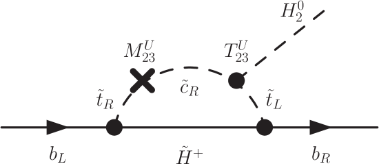
Figure 3: Quark-flavour violating mass insertions to the vertex graph $H^{0}_{2}\to b\bar{b}$ with charged higgsino loop, proportional to $h_{b}h_{t}$, see eqs. (55) and (47).

4.2 Gluino and chargino contributions to $h^{0}\to b\bar{b}$

We decompose the bottom self energy $\Sigma_{b}$ defined by the Lagrangian ${\cal L}=-\bar{b}\,\Sigma_{b}\,b$ as follows

$$\Sigma_{b}(p)=\not{p}\left(\Sigma^{LL}_{b}(p^{2})P_{L}+\Sigma^{RR}_{b}(p^{2})P_{R}\right)+m_{b}\left(\Sigma^{RL}_{b}(p^{2})P_{L}+\Sigma^{LR}_{b}(p^{2})P_{R}\right)\,,$$ (38)

with $\Sigma^{LR}_{b}=\Sigma^{RL*}_{b}$. We have $\Sigma^{LR}_{b}=\Sigma^{RL}_{b}$, as we assume real input parameters, and

$$m_{b}\Sigma^{LR,\tilde{g}}_{b}=-\frac{2\alpha_{s}}{3\pi}m_{\tilde{g}}\,\sum_{i=1}^{6}U^{\tilde{d}*}_{i3}U^{\tilde{d}}_{i6}B_{0}(m_{b}^{2},m^{2}_{\tilde{g}},m^{2}_{\tilde{d}_{i}})\,.$$ (39)

Allowing the squared $\tilde{d}$-mass matrix in the form

$${\cal M}^{2}_{\tilde{d}}=\left(\begin{array}[]{cc}{\cal M}^{2}_{\tilde{d},LL}&{\cal M}^{2}_{\tilde{d},LR}\\[5.69054pt] {\cal M}^{2}_{\tilde{d},RL}&{\cal M}^{2}_{\tilde{d},RR}\end{array}\right)\equiv M_{ij}=\left(\begin{array}[]{cccccc}M^{LL}_{11}&0&0&0&0&0\\ 0&M^{LL}_{22}&M^{Q}_{23}&0&0&\hat{v}_{1}T^{D}_{32}\\ 0&M^{Q}_{23}&M^{LL}_{33}&0&\hat{v}_{1}T^{D}_{23}&M^{RL}_{33}\\ 0&0&0&M^{RR}_{11}&0&0\\ 0&0&\hat{v}_{1}T^{D}_{23}&0&M^{RR}_{22}&M^{D}_{23}\\ 0&\hat{v}_{1}T^{D}_{32}&M^{RL}_{33}&0&M^{D}_{23}&M^{RR}_{33}\end{array}\right)\,,$$ (40)

with $M^{RL}_{33}\sim-\mu m_{b}\tan\beta$, $\hat{v}_{1}=v\cos\beta/\sqrt{2}\sim$ 170 GeV$/\tan\beta$, and the QFV elements of the $3\times 3$ matrices $M^{2}_{Q}$ and $M^{2}_{D}$ are written as $M^{Q}_{ij}$ and $M^{D}_{ij}$, respectively. Using eq. (15) we get

$$m_{b}\Sigma^{LR,\tilde{g}}_{b}=-\frac{2\alpha_{s}}{3\pi}m_{\tilde{g}}(T^{FC}_{1}+T^{FV}_{2}+T^{FC}_{3}+T^{FV}_{3}+\ldots)$$ (41)

where the quark flavour conserving (FC) and quark flavour violating (FV) contributions read

$$T^{FC}_{1} = M^{RL}_{33}\,b_{0}\!\left(1,m_{\tilde{g}}^{2},\{M^{RR}_{33},M^{LL}_{33}\}\right)$$

$$T^{FV}_{2} = \hat{v}_{1}T^{D}_{32}M^{Q}_{23}\,b_{0}\!\left(2,m_{\tilde{g}}^{2},\{M^{RR}_{33},M^{LL}_{22},M^{LL}_{33}\}\right)$$

$$+ \hat{v}_{1}T^{D}_{23}M^{D}_{23}\,b_{0}\!\left(2,m_{\tilde{g}}^{2},\{M^{RR}_{33},M^{RR}_{22},M^{LL}_{33}\}\right)$$

$$T^{FC}_{3} = 3^{\rho}\,(M^{RL}_{33})^{3}\,b_{0}\!\left(3,m_{\tilde{g}}^{2},\{M^{RR}_{33},M^{LL}_{33},M^{RR}_{33},M^{LL}_{33}\}\right)$$

$$T^{FV}_{3} = (M^{Q}_{23})^{2}M^{RL}_{33}\,b_{0}\!\left(3,m_{\tilde{g}}^{2},\{M^{RR}_{33},M^{LL}_{33},M^{LL}_{22},M^{LL}_{33}\}\right)$$ (42)

$$+ (M^{D}_{23})^{2}M^{RL}_{33}\,b_{0}\!\left(3,m_{\tilde{g}}^{2},\{M^{RR}_{33},M^{RR}_{33},M^{RR}_{22},M^{LL}_{33}\}\right)$$

$$+ 3^{\rho}\,(\hat{v}_{1})^{2}(T^{D}_{32})^{2}M^{RL}_{33}\,b_{0}\!\left(3,m_{\tilde{g}}^{2},\{M^{RR}_{33},M^{LL}_{22},M^{RR}_{33},M^{LL}_{33}\}\right)$$

$$+ 3^{\rho}\,(\hat{v}_{1})^{2}(T^{D}_{23})^{2}M^{RL}_{33}\,b_{0}\!\left(3,m_{\tilde{g}}^{2},\{M^{RR}_{33},M^{LL}_{33},M^{RR}_{22},M^{LL}_{33}\}\right)\,,$$

with $\rho=0$. As in the charm sector, the vertex contribution can be directly deduced from the self energy, $T^{v\,x}_{i}={T^{x}_{i}\over\hat{v}_{1}},x={FC,FV}$, with an additional factor 3 for some terms in $T^{x}_{3}$, $(M^{RL}_{33})^{3}\to 3(M^{RL}_{33})^{3}$, $(T^{D}_{23})^{2}M^{RL}_{33}\to 3(T^{D}_{23})^{2}M^{RL}_{33}$, $(T^{D}_{32})^{2}M^{RL}_{33}\to 3(T^{D}_{32})^{2}M^{RL}_{33}$, and accordingly $\rho=1$. The interactions related to the mass insertions are given by

$${\cal L} = -T^{D}_{33}\,{\tilde{b}}_{R}^{*}{\tilde{b}}_{L}H^{0}_{1}-T^{D}_{32}\,{\tilde{b}}_{R}^{*}{\tilde{s}}_{L}H^{0}_{1}-T^{D}_{23}\,{\tilde{s}}_{R}^{*}{\tilde{b}}_{L}H^{0}_{1}-M^{RL}_{33}\,{\tilde{b}}_{L}^{*}{\tilde{b}}_{R}-M^{Q}_{23}\,{\tilde{b}}_{L}^{*}{\tilde{s}}_{L}$$ (43)

$$-M^{D}_{23}\,{\tilde{b}}_{R}^{*}{\tilde{s}}_{R}+{\rm h.c.}\,,$$

with $H^{0}_{1}={1\over\sqrt{2}}(v\cos\beta-h^{0}\sin\alpha+\ldots)$.

We will apply the mass insertion technique for the self-energy amplitude of the bottom-quark and for the vertex amplitude with a chargino in the loop. The relevant term for the self energy calculation is proportional to $c^{*}_{L}c_{R}$, with $c_{L}=h_{b}U^{*}_{m2}U^{\tilde{u}*}_{i3}$ and $c_{R}=-gV_{m1}U^{\tilde{u}*}_{i3}+h_{t}V_{m2}U^{\tilde{u}*}_{i6}$. Using eq. (38) we get

$$m_{b}\Sigma^{LR,\tilde{\chi}^{+}}_{b} = {1\over 16\pi^{2}}\sum_{m=1}^{2}\sum_{i=1}^{6}m_{\tilde{\chi}^{+}_{m}}\left(-gh_{b}U_{m2}V_{m1}|U^{\tilde{u}}_{i3}|^{2}+h_{b}h_{t}U_{m2}V_{m2}U^{\tilde{u}}_{i3}U^{\tilde{u}*}_{i6}\right)\times$$ (44)

$$\hskip 199.16928ptB_{0}(m_{b}^{2},m^{2}_{\tilde{\chi}^{+}_{m}},m^{2}_{\tilde{u}_{i}})\,.$$

Neglecting the term proportional to the SU(2) coupling $g$ and the bottom mass in the loop integrals, we get

$$m_{b}\Sigma^{LR,\tilde{\chi}^{+}}_{b}={h_{b}h_{t}\over 16\pi^{2}}\sum_{m=1}^{2}\sum_{i=1}^{6}m_{\tilde{\chi}^{+}_{m}}U_{m2}V_{m2}\,U^{\tilde{u}}_{i3}U^{\tilde{u}*}_{i6}b_{0}(m^{2}_{\tilde{\chi}^{+}_{m}},m^{2}_{\tilde{u}_{i}})\,.$$ (45)

Concerning the mass insertions in the $\tilde{u}_{i}$ line, we have the same structure as in eq. (39), but for the $\tilde{u}$ sector. We have $M^{RL}_{33}\to\hat{v}_{2}T^{U}_{33}$, $T^{D}\to T^{U}$, and $M^{D}_{23}\to M^{U}_{23}$. Therefore, we can use the results for the bottom self energy with gluino in the loop. Using eq. (23) we obtain

$$m_{b}\Sigma^{LR,\tilde{\chi}^{+}}_{b}={h_{b}h_{t}\over 16\pi^{2}}\sum_{m=1}^{2}m_{\tilde{\chi}^{+}_{m}}U_{m2}V_{m2}\,\left(T^{FC}_{1}+T^{FV}_{2}+T^{FC}_{3}+T^{FV}_{3}+\ldots\right)\,,$$ (46)

where

$$T^{FC}_{1} = \hat{v}_{2}T^{U}_{33}\,b_{0}\!\left(1,m_{\tilde{\chi}^{+}_{m}}^{2},\{M^{RR}_{33},M^{LL}_{33}\}\right)$$

$$T^{FV}_{2} = \hat{v}_{2}T^{U}_{32}M^{Q}_{23}\,b_{0}\!\left(2,m_{\tilde{\chi}^{+}_{m}}^{2},\{M^{RR}_{33},M^{LL}_{22},M^{LL}_{33}\}\right)$$

$$+ \hat{v}_{2}T^{U}_{23}M^{U}_{23}\,b_{0}\!\left(2,m_{\tilde{\chi}^{+}_{m}}^{2},\{M^{RR}_{33},M^{RR}_{22},M^{LL}_{33}\}\right)$$

$$T^{FC}_{3} = 3^{\rho}\,(\hat{v}_{2}T^{U}_{33})^{3}\,b_{0}\!\left(3,m_{\tilde{\chi}^{+}_{m}}^{2},\{M^{RR}_{33},M^{LL}_{33},M^{RR}_{33},M^{LL}_{33}\}\right)$$

$$T^{FV}_{3} = \hat{v}_{2}T^{U}_{33}(M^{Q}_{23})^{2}\,b_{0}\!\left(3,m_{\tilde{\chi}^{+}_{m}}^{2},\{M^{RR}_{33},M^{LL}_{33},M^{LL}_{22},M^{LL}_{33}\}\right)$$ (47)

$$+ \hat{v}_{2}T^{U}_{33}(M^{U}_{23})^{2}\,b_{0}\!\left(3,m_{\tilde{\chi}^{+}_{m}}^{2},\{M^{RR}_{33},M^{RR}_{33},M^{RR}_{22},M^{LL}_{33}\}\right)$$

$$+ 3^{\rho}\,(\hat{v}_{2})^{3}(T^{U}_{32})^{2}\,T^{U}_{33}\,b_{0}\!\left(3,m_{\tilde{\chi}^{+}_{m}}^{2},\{M^{RR}_{33},M^{LL}_{22},M^{RR}_{33},M^{LL}_{33}\}\right)$$

$$+ 3^{\rho}\,(\hat{v}_{2})^{3}(T^{U}_{23})^{2}\,T^{U}_{33}\,b_{0}\!\left(3,m_{\tilde{\chi}^{+}_{m}}^{2},\{M^{RR}_{33},M^{LL}_{33},M^{RR}_{22},M^{LL}_{33}\}\right)\,,$$

with $\rho=0$. The graphs corresponding to $T_{1}$, $T_{2}$ and $T_{3}$ are shown in Figs. 3, (3, 3) and (3-3), respectively. Furthermore, we also apply the mass insertion technique to the chargino part in eq. (46). The eigenvalue equation is $U^{*}XV^{-1}=M_{D}={\rm diag}(m_{\tilde{\chi}^{+}_{1}},m_{\tilde{\chi}^{+}_{2}})$. We assume the chargino mass matrix to be real,

$$X = \left(\begin{array}[]{cc}M_{2}&\sqrt{2}m_{W}\sin\beta\\ \sqrt{2}m_{W}\cos\beta&\mu\end{array}\right)\,,$$ (50)

$${(X^{2})}\equiv X^{\dagger}X = \left(\begin{array}[]{cc}M_{2}^{2}+2m^{2}_{W}\cos^{2}\beta&\sqrt{2}m_{W}(\mu\cos\beta+M_{2}\sin\beta)\\ \sqrt{2}m_{W}(\mu\cos\beta+M_{2}\sin\beta)&\mu^{2}+2m^{2}_{W}\sin^{2}\beta\end{array}\right)\,.$$ (53)

The formula with linear mass insertion reads

$$\sum_{m=1}^{2}m_{\tilde{\chi}^{+}_{m}}U_{m2}V_{m2}\,f(m^{2}_{\tilde{\chi}^{+}_{m}})=X_{22}f({(X^{2})}_{22})+X_{21}{(X^{2})}_{21}{f({(X^{2})}_{22})-f({(X^{2})}_{11})\over{(X^{2})}_{22}-{(X^{2})}_{11}}\,.$$ (54)

Assuming $m_{W}\ll M_{2},\mu$, the linear term vanishes, and $X_{22}f({(X^{2})}_{22})\sim\mu f(\mu^{2})$. We get the final approximate result

$$m_{b}\Sigma^{LR,\tilde{\chi}^{+}}_{b}={h_{b}h_{t}\over 16\pi^{2}}\mu\,\left(T^{FC}_{1}+T^{FV}_{2}+T^{FC}_{3}+T^{FV}_{3}+\ldots\right)\,,$$ (55)

with the terms $T^{x}_{i}$ taken from eq. (47) with $m_{\tilde{\chi}^{+}_{m}}^{2}\to\mu^{2}$.

Neglecting the wave-function renormalization contributions, which are proportional to the tree-level coupling $s^{1}_{b}$ we get the approximate result for the decay $h^{0}\to b\bar{b}$,

$$\Gamma^{\rm appr}(h^{0}\to b\bar{b})=\Gamma^{g,{\rm impr}}-2\left(\Sigma^{LR,\tilde{g}}_{b}+\Sigma^{LR,\tilde{\chi}^{+}}_{b}\right)\,\Gamma^{\rm tree}(m_{b})\,,$$ (56)

where $\Sigma^{LR,\tilde{g}}_{b}$ and $\Sigma^{LR,\tilde{\chi}^{+}}_{b}$ are given in eq. (39) and eq. (44) or in the MI-approximation in eq. (41) and eq. (55), respectively, with $\rho=1$. $\Gamma^{g,{\rm impr}}$ is given by eq. (55) and $\Gamma^{\rm tree}$ by eq. (9) in Bartl:2014bka , with $c\to b$.

In Crivellin:2010er the chirally enhanced corrections to Higgs vertices in the most general MSSM were discussed analytically by taking into account gluino-squark loops. We qualitatively agree with their results on $h^{0}\to b\bar{b}$. A study including two-loop SUSY-QCD corrections was performed in Crivellin:2012zz .

5 Numerical results

In this section we demonstrate the effects of QFV due to $\tilde{c}-\tilde{t}$ mixing in the decays of $h^{0}$ to $b\bar{b}$ and $c\bar{c}$ in the MSSM. In order to find an explicit scenario where both decay widths deviate appreciably from the SM values, we have performed two scans over wide parameter regions. In the first calculation we have scanned 8750000 parameter points. From them only 17% have satisfied the existing theoretical and experimental constraints (see Appendix B). The parameters involved and their variations are given as follows:

$$\{M^{2}_{U11},M^{2}_{U22},M^{2}_{U33}\}~{}[{\rm GeV}^{2}] = ~{}{\rm in~{}sets~{}of}~{}\bigg{\{}\{2400^{2},2300^{2},1800^{2}\},$$

$$\{3000^{2},2800^{2},2000^{2}\},\{3200^{2},3000^{2},2200^{2}\},$$

$$\{2400^{2},1100^{2},1000^{2}\},\{3200^{2},2200^{2},2000^{2}\}\bigg{\}};$$

$$\{M^{2}_{Q11},M^{2}_{Q22},M^{2}_{Q33}\} = \{M^{2}_{U11},M^{2}_{U22},M^{2}_{U33}\};$$

$$\tan\beta = \{15\div 30\}~{}{\rm with~{}step~{}size}~{}2.5;$$

$$\mu~{}[{\rm GeV}] = \{1200\div 2200\}~{}{\rm with~{}step~{}size}~{}250;$$

$$\{M_{1},M_{2},M_{3}\}~{}[{\rm GeV}] = ~{}{\rm in~{}sets~{}of}~{}\bigg{\{}\{300,600,1800\},\{400,800,2000\},$$

$$\{500,1000,2200\},\{600,1200,2200\},$$

$$\{700,1400,2400\}\bigg{\}};$$

$$M^{2}_{U23}~{}[{\rm GeV}^{2}] = \{-2430^{2}\div 2430^{2}\}~{}{\rm with~{}step~{}size}~{}\approx 1\times 10^{6};$$

$$M^{2}_{Q23}~{}[{\rm GeV}^{2}] = \{-1140^{2}\div 1140^{2}\}~{}{\rm with~{}step~{}size}~{}\approx 2.9\times 10^{5};$$

$$T_{U23}~{}[{\rm GeV}] = \{-3000\div 3000\}~{}{\rm with~{}step~{}size}~{}400;$$

$$T_{U32}~{}[{\rm GeV}] = \{-3000\div 3000\}~{}{\rm with~{}step~{}size}~{}400.$$ (57)

In the second calculation we have varied in more detail the parameters of the mass matrices $M_{U}$ and $M_{Q}$, which in the first step have been assumed to change only simultaneously in sets of equal diagonal elements, $(M_{U})_{ii}=(M_{Q})_{ii}$, for $i=1,2,3$. In this calculation we have scanned 9834496 points and 12% of them have survived the constraints. The parameters involved and their variations are given by:

$$M^{2}_{U22}~{}[{\rm GeV}^{2}] = \{1000^{2}\div 3200^{2}\}~{}{\rm with~{}step~{}size}~{}\approx 1.3\times 10^{6};$$

$$M^{2}_{U33}~{}[{\rm GeV}^{2}] = \{970^{2}\div 3100^{2}\}~{}{\rm with~{}step~{}size}~{}1.2\times 10^{6};$$

$$M^{2}_{Q22}~{}[{\rm GeV}^{2}] = \{950^{2}\div 3150^{2}\}~{}{\rm with~{}step~{}size}~{}\approx 1.5\times 10^{6};$$

$$M^{2}_{Q33}~{}[{\rm GeV}^{2}] = \{1100^{2}\div 3100^{2}\}~{}{\rm with~{}step~{}size}~{}1.4\times 10^{6};$$

$$M^{2}_{U23}~{}[{\rm GeV}^{2}] = \{-2400^{2}\div 2400^{2}\}~{}{\rm with~{}step~{}size}~{}\approx 1.6\times 10^{6};$$

$$M^{2}_{Q23}~{}[{\rm GeV}^{2}] = \{-1150^{2}\div 1150^{2}\}~{}{\rm with~{}step~{}size}~{}\approx 4.4\times 10^{5};$$

$$T_{U23}~{}[{\rm GeV}] = \{-3000\div 3000\}~{}{\rm with~{}step~{}size}~{}\approx 1\times 10^{3};$$

$$T_{U32}~{}[{\rm GeV}] = \{-3000\div 3000\}~{}{\rm with~{}step~{}size}~{}\approx 850.$$ (58)

In both scans the following parameters have been fixed: $M^{2}_{D11}=1.024\times 10^{7}~{}{\rm GeV}^{2},M^{2}_{D22}=9\times 10^{6}~{}{\rm GeV}^{2},M^{2}_{D33}\approx 7\times 10^{6}~{}{\rm GeV}^{2},T_{U33}=2000~{}{\rm GeV},M^{2}_{D23}=M^{2}_{D32}=T_{D23}=T_{D32}=T_{D33}=0$. In the second scan we have also fixed the parameters: $M_{1}=400~{}{\rm GeV},M_{2}=800~{}{\rm GeV},M_{3}=2000~{}{\rm GeV},\mu=1800~{}{\rm GeV},\tan\beta=30,M^{2}_{U11}=M^{2}_{Q11}=1.024\times 10^{7}~{}{\rm GeV}^{2}.$ A detailed study of the MSSM QFV parameter space has also been done in DeCausmaecker:2015yca .

The results of the scans are summarised in Fig. 4, where the distributions of the deviation from the SM width for $h^{0}\to b\bar{b}$ and $h^{0}\to c\bar{c}$ are shown. We take $\Gamma^{\rm SM}(h^{0}\to b\bar{b})=2.35$ MeV Almeida:2013jfa , $\Gamma^{\rm SM}(h^{0}\to c\bar{c})=0.118$ MeV pdg2014 , $m_{b}(m_{b})^{{\overline{\rm MS}}}=4.2~{}{\rm GeV},m_{c}(m_{c})^{{\overline{\rm MS}}}=1.275~{}{\rm GeV}$ PDG2013 , and $\alpha_{s}(m_{Z})=0.1185$ a_s@ICHEP2014 . The y-axis counts the number of survived parameter points for each bin of the deviation. It is seen that in the case of $h^{0}\to b\bar{b}$ (Fig. 4) the detailed variation of the elements $M_{U}$ and $M_{Q}$ can increase the effect and the deviation from the SM can go up to $\sim 30\%$ at certain parameter points. In the case of $h^{0}\to c\bar{c}$ (Fig. 4) a large deviation from the SM value due to large values of the product $T^{U}_{32}M^{U}_{23}$, discussed at the end of Section 3.2, is in principle possible. Since there exists no physical constraint on this product we will only show results with a deviation from the SM up to $\sim\pm 50\%$.

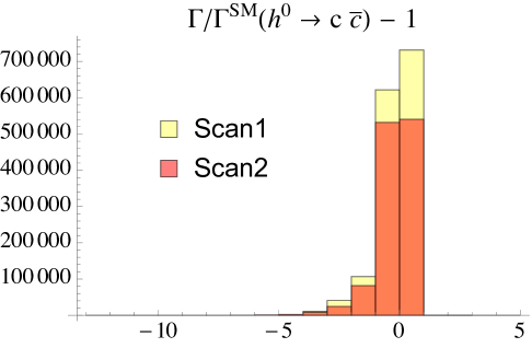
Figure 4: Distribution of the results for the deviation from the SM (a) $\Gamma$/$\Gamma^{\rm SM}(h^{0}\to b\bar{b})-1$ and (b) $\Gamma$/$\Gamma^{\rm SM}(h^{0}\to c\bar{c})-1$ from Scan 1 and Scan 2.

Table 1: Reference scenario: shown are the basic MSSM parameters at $Q=1$ TeV, except for $m_{A^{0}}$ which is the pole mass (i.e. the physical mass) of $A^{0}$, with $T_{U33}=1450$ GeV (corresponding to $\delta^{uRL}_{33}=0.1$). All other squark parameters not shown here are zero.

$M_{1}$	$M_{2}$	$M_{3}$
400  GeV	800  GeV	2000 GeV

$\mu$	$\tan\beta$	$m_{A^{0}}$
500 GeV	30	1500  GeV

	$\alpha=1$	$\alpha=2$	$\alpha=3$
$M_{Q\alpha\alpha}^{2}$	$3200^{2}~{}{\rm GeV}^{2}$	$1550^{2}~{}{\rm GeV}^{2}$	$1100^{2}~{}{\rm GeV}^{2}$
$M_{U\alpha\alpha}^{2}$	$3200^{2}~{}{\rm GeV}^{2}$	$2800^{2}~{}{\rm GeV}^{2}$	$2050^{2}~{}{\rm GeV}^{2}$
$M_{D\alpha\alpha}^{2}$	$3200^{2}~{}{\rm GeV}^{2}$	$3000^{2}~{}{\rm GeV}^{2}$	$2500^{2}~{}{\rm GeV}^{2}$

$\delta^{LL}_{23}$	$\delta^{uRR}_{23}$	$\delta^{uRL}_{23}$	$\delta^{uLR}_{23}$
0	0.8	0.02	0.02

Based on the results from the scans we have chosen a reference scenario with strong $\tilde{c}-\tilde{t}$ mixing to demonstrate the effects of QFV in both $h^{0}$ to $b\bar{b}$ and $c\bar{c}$ decays. The corresponding MSSM parameters at $Q=1$ TeV are given in Table 1.

Table 2: Physical masses in GeV of the particles for the scenario of Table 1.

$m_{\tilde{\chi}^{0}_{1}}$	$m_{\tilde{\chi}^{0}_{2}}$	$m_{\tilde{\chi}^{0}_{3}}$	$m_{\tilde{\chi}^{0}_{4}}$	$m_{\tilde{\chi}^{+}_{1}}$	$m_{\tilde{\chi}^{+}_{2}}$
$395$	$507$	$511$	$845$	$501$	$845$

$m_{h^{0}}$	$m_{H^{0}}$	$m_{A^{0}}$	$m_{H^{+}}$
$125$	$1500$	$1500$	$1503$

$m_{\tilde{g}}$	$m_{\tilde{u}_{1}}$	$m_{\tilde{u}_{2}}$	$m_{\tilde{u}_{3}}$	$m_{\tilde{u}_{4}}$	$m_{\tilde{u}_{5}}$	$m_{\tilde{u}_{6}}$
$2103$	$996$	$1176$	$1578$	$3214$	$3217$	$3327$

$m_{\tilde{d}_{1}}$	$m_{\tilde{d}_{2}}$	$m_{\tilde{d}_{3}}$	$m_{\tilde{d}_{4}}$	$m_{\tilde{d}_{5}}$	$m_{\tilde{d}_{6}}$
$1128$	$1579$	$2515$	$3012$	$3211$	$3218$

Table 3: Flavour decomposition of $\tilde{u}_{i}$, $i=1,...,6$ for the scenario of Table 1. Shown are the squared coefficients.

	$\tilde{u}_{L}$	$\tilde{c}_{L}$	$\tilde{t}_{L}$	$\tilde{u}_{R}$	$\tilde{c}_{R}$	$\tilde{t}_{R}$
$\tilde{u}_{1}$	$0$	$0.002$	$0.25$	$0$	$0.228$	$0.52$
$\tilde{u}_{2}$	$0$	$0$	$0.749$	$0$	$0.086$	$0.165$
$\tilde{u}_{3}$	$0.051$	$0.946$	$0.001$	$0$	$0$	$0$
$\tilde{u}_{4}$	$0.95$	$0.05$	$0$	$0$	$0$	$0$
$\tilde{u}_{5}$	$0$	$0$	$0$	$1$	$0$	$0$
$\tilde{u}_{6}$	$0$	$0$	$0$	$0$	$0.69$	$0.31$

This scenario satisfies all present experimental and theoretical constraints, see Appendix B. The resulting physical masses of the particles are shown in Table 2. We also show the flavour decomposition of the up-type squarks $\tilde{u}_{i},i=1,...,6$ in Table 3. For the calculation of the masses and the mixing, as well as for the low-energy observables, especially those in the B meson sector (see Table 4), we use the public code SPheno v3.3.3 SPheno1 ; SPheno2 . Both the widths $\Gamma(h^{0}\to b\bar{b})$ and $\Gamma(h^{0}\to c\bar{c})$ are calculated at full one-loop level in the MSSM with QFV using the packages FeynArts Hahn:2000kx and FormCalc Hahn:1998yk . We also use the packages SSP SSP and LoopTools Hahn:1998yk . For creating the Fortran code for the mass insertion formulas MassToMI arXiv:1509.05030 was very helpful. In the following unless specified otherwise we show various parameter dependences of $\Gamma/\Gamma^{\rm SM}-1$ for $\Gamma(h^{0}\to b\bar{b})$ and $\Gamma(h^{0}\to c\bar{c})$ with all other parameters fixed as in Table 1.

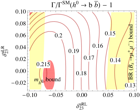
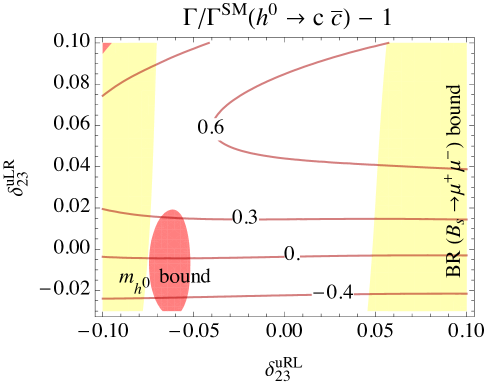
Figure 5: Contours of the deviation (a) $\Gamma/\Gamma^{\rm SM}(h^{0}\to b\bar{b})-1$ and (b) $\Gamma/\Gamma^{\rm SM}(h^{0}\to c\bar{c})-1$ in the $\delta^{uRL}_{23}$-$\delta^{uLR}_{23}$ plane for $\delta^{uRR}_{23}=0.5$ and $\delta^{LL}_{23}=0$.

In Fig. 5 the dependence on the QFV parameters $\delta^{uRL}_{23}$ and $\delta^{uLR}_{23}$ is shown. It is seen that in the case of $b\bar{b}$ (Fig. 5) the variation due to correlated $\tilde{c}_{R}-\tilde{t}_{L}$ and $\tilde{c}_{L}-\tilde{t}_{R}$ mixing can vary up to $\sim 6\%$ in the region allowed by the constraints. Comparing Fig. 5 with Fig. 5 one can see that there exist regions where both widths considered simultaneously deviate from their SM prediction. Hence $\Gamma(h^{0}\to b\bar{b})$ tends to depend more on $\tilde{c}_{R}-\tilde{t}_{L}$ mixing, while $\Gamma(h^{0}\to c\bar{c})$ depends more on $\tilde{c}_{L}-\tilde{t}_{R}$ mixing.

This tendency can also be seen in Fig. 6. On the left hand side (Fig. 6) the dependence of $\Gamma/\Gamma^{\rm SM}(h^{0}\to b\bar{b})$ on the QFV parameters $\delta^{uRR}_{23}$ and $\delta^{uRL}_{23}$ is shown. The variation due to $\tilde{c}_{R}-\tilde{t}_{L}$ and $\tilde{c}_{R}-\tilde{t}_{R}$ mixing is $\sim 7\%$. In the same scenario, however, the variation of $\Gamma/\Gamma^{\rm SM}(h^{0}\to c\bar{c})$ (not shown here) is only $\sim 3\%$. On the right hand side (Fig. 6) $\Gamma/\Gamma^{\rm SM}(h^{0}\to c\bar{c})$ is shown as a function of $\delta^{uRR}_{23}$ and $\delta^{uLR}_{23}$. The variation is large and can go up to $\sim 30\%$, see also Bartl:2014bka . In the same scenario, however, $\Gamma/\Gamma^{\rm SM}(h^{0}\to b\bar{b})$ varies only by less than one percent.

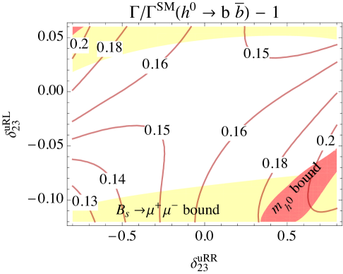
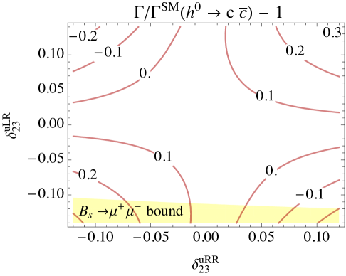
Figure 6: Contours of the deviation (a) $\Gamma/\Gamma^{\rm SM}(h^{0}\to b\bar{b})-1$ in the $\delta^{uRR}_{23}$-$\delta^{uRL}_{23}$ plane for $\delta^{LL}_{23}=0$ and $\delta^{uLR}_{23}=0$ and (b) $\Gamma/\Gamma^{\rm SM}(h^{0}\to c\bar{c})-1$ in the $\delta^{uRR}_{23}$-$\delta^{uLR}_{23}$ plane for $\delta^{LL}_{23}=0$ and $\delta^{uRL}_{23}=0.02$.

In Section 4.1, in agreement with our results in Ref. Bartl:2014bka , we have shown that in the case of $c\bar{c}$ the deviation from the SM is entirely due to QFV. However, it is known that in the MSSM $\Gamma(h^{0}\to b\bar{b})$ can differ considerably from the SM due to QFC contributions Endo:2015oia . In Fig. 7 the individual contributions to $\Gamma/\Gamma^{\rm SM}(h^{0}\to b\bar{b})$ (i.e. QFC gluino one-loop, QFC and QFV chargino one-loop contributions computed in the mass insertion approximation) are shown as a function of $\delta^{uRL}_{23}$ for the parameters of Fig. 5 with $\delta^{uRL}_{23}$=0.02. The QFC/QFV gluino and chargino one-loop contributions in the mass insertion approximation are given in Section 4. The $"h^{0}"$ contribution denotes $\Gamma^{g,\rm impr}/\Gamma^{\rm SM}(h^{0}\to b\bar{b})-1$ which depends on $m_{h^{0}}$ and the angle $\alpha$ and hence depends on both the QFC and QFV parameters. Note that $m_{h^{0}}$ as well as $\sin\alpha$ already appear in the kinematics factor at tree level, see eq. (11). The top curve shows the deviation of the full one-loop level width of eq. (13) from the SM width, $\Gamma/\Gamma^{\rm SM}(h^{0}\to b\bar{b})-1$, with no approximation. It is seen that the main one-loop contributions to $\Gamma(h^{0}\to b\bar{b})$ come from QFC gluino and QFC chargino exchange. Nevertheless, there exists a region for large and negative $\delta^{uRL}_{23}$ where the QFV component can be comparable with the QFC component. The QFV component is mainly due to chargino exchange which involves mixing in the $\tilde{u}$ sector. On the other hand, in the $b\bar{b}$ case the gluino exchange, which plays a major role in the $c\bar{c}$ case, involves $\tilde{d}$ quarks whose QFV mixing effect is strongly suppressed, and hence the QFV component of the gluino exchange contribution is very small. Therefore, it is not shown in this figure. It is also interesting that the $"h^{0}"$ contribution depends significantly on the QFV parameter $\delta^{uRL}_{23}$. After all, the variation of $\Gamma/\Gamma^{\rm SM}(h^{0}\to b\bar{b})$ in the shown QFV parameter range, which can be taken as QFV effect, can be as large as $\sim 7\%.$

Fig.7 demonstrates the quality of our approximated result (56). By comparing numerically the different MI orders we realized that the MI formulas converge fast for $\tilde{g}$ FC and $\tilde{\chi}^{+}$ FC, but not for $\tilde{\chi}^{+}$ FV. This can be seen by comparing Fig. 7 with Fig. 7. Thus, the difference between the dotted curve and the upper curve in Fig. 7 is mainly due to the relatively slow MI convergence of the $\tilde{\chi}^{+}$ FV contribution.

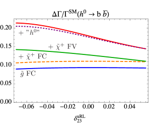
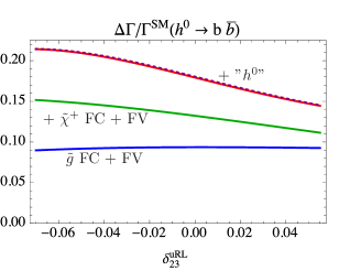
Figure 7: (a) The QFV and QFC gluino and chargino one-loop contributions (added from bottom to top) to $\Gamma/\Gamma^{\rm SM}(h^{0}\to b\bar{b})$ computed by using the mass insertion technique, see Section 4, as a function of $\delta^{uRL}_{23}$ for the parameters of Fig. 5 with $\delta^{uLR}_{23}=0.02$. (b) The total gluino and chargino one-loop contributions to $\Gamma/\Gamma^{\rm SM}(h^{0}\to b\bar{b})$ computed by using the approximate formula (56) together with eq. (39) and the finite part of eq. (44) as a function of $\delta^{uRL}_{23}$ for the same parameters as in (a). In both graphs the "$h^{0}$" contribution denotes $\Gamma^{g,\rm imp}/\Gamma^{\rm SM}(h^{0}\to b\bar{b})-1$ and the top curve shows deviation of the full one-loop level width of eq. (13) from the SM width, $\Gamma/\Gamma^{\rm SM}(h^{0}\to b\bar{b})-1$, with no approximation.

Although the decay $h^{0}\to b\bar{b}$ is dominant, the measurement of its branching ratio and width at the LHC will be a big challenge. At LHC one always measures $\sigma(pp\to h^{0}X){\rm B}(h^{0}\to b\bar{b})$. The largest Higgs boson production cross section is due to gluon gluon fusion. However, due to the huge QCD background it will be difficult to isolate the $h^{0}\to b\bar{b}$ mode. The other production modes (vector boson fusion, Higgs radiation from $W^{\pm}Z$, and associated $t\bar{t}h^{0}$ production) have smaller cross sections, but may have less background. In any case, high luminosity at LHC would be needed CMS:2013xfa . A model independent and precise measurement of B($h^{0}\to b\bar{b}$) and $\Gamma(h^{0}\to b\bar{b})$ would be possible at a $e^{+}e^{-}$ linear collider such as ILC Barklow:2015tja .

6 Conclusions

In analogy to our previous paper Bartl:2014bka , we have calculated the decay width of $h^{0}\to b\bar{b}$ in the MSSM with quark flavour violation at full one-loop level. We have studied the effects of $\tilde{c}-\tilde{t}$ mixing, taking into account all constraints on the QFV parameters from B-meson data. We have discussed in detail both the decays $h^{0}\to c\bar{c}$ and $h^{0}\to b\bar{b}$ within the perturbative mass insertion technique applying the Flavour Expansion Theorem Dedes:2015twa . There are cases, where the charm self-energy and consequently the correction to the width $\Gamma(h^{0}\to c\bar{c})$ can become unacceptably large. This is due to the product $M^{U}_{23}T^{U}_{32}$, for which there exists no bound. In general, the deviation of $\Gamma(h^{0}\to b\bar{b})$ from the SM can be large (up to 30%), mainly coming from the QFC part of the MSSM. The QFV contribution due to $\tilde{c}_{L,R}-\tilde{t}_{L,R}$ mixing and chargino exchange is smaller but can nevertheless reach $\sim 7\%$ at certain parameter points. The QFV part due to gluino exchange, which is due to $\tilde{s}_{L,R}-\tilde{b}_{L,R}$ mixing, is very small.

Appendix A Interaction Lagrangian

• In the MSSM the interaction of the lightest neutral Higgs boson, $h^{0}$, with two bottom quarks is given by

  $${\cal L}_{h^{0}b\bar{b}}=s_{1}^{b}h^{0}\bar{b}b\,,$$ (59)

  with the tree-level coupling $s_{1}^{b}$ given by eq. (12).

• In the super-CKM basis, the interaction of the lightest neutral Higgs boson, $h^{0}$, with two down-type squarks is given by

  $${\cal L}_{h^{0}\tilde{d}_{i}\tilde{d}_{j}}=G_{ij1}^{\tilde{d}}h^{0}\tilde{d}_{j}^{*}\tilde{d}_{i},\,~{}i,j=1,...,6.$$ (60)

  The coupling $G_{ij1}^{\tilde{d}}$ reads

  $$G_{ij1}^{\tilde{d}}=\frac{g}{2m_{W}}\,\bigg{[}-m_{W}^{2}\sin(\alpha+\beta)\Big{[}(1+\tfrac{1}{3}\tan^{2}\theta_{\textit{\tiny{W}}})$$

  $$\times(U^{\tilde{d}})_{jk}(U^{\tilde{d}*})_{ik}+\tfrac{2}{3}\tan^{2}\theta_{\textit{\tiny{W}}}(U^{\tilde{d}})_{j\,(k+3)}(U^{\tilde{d}*})_{i\,(k+3)}\Big{]}$$

  $$+\ 2\dfrac{\sin\alpha}{\cos\beta}\Big{[}(U^{\tilde{d}})_{jk}\ m^{2}_{d,k}(U^{\tilde{d}*})_{ik}+(U^{\tilde{d}})_{j\,(k+3)}m^{2}_{d,k}(U^{\tilde{d}*})_{i\,(k+3)}\Big{]}$$

  $$+\ \dfrac{\cos\alpha}{\cos\beta}\Big{[}\mu^{*}(U^{\tilde{d}})_{j\,(k+3)}m_{d,k}(U^{\tilde{d}*})_{ik}+\mu(U^{\tilde{d}})_{jk}m_{d,k}(U^{\tilde{d}*})_{i\,(k+3)}\Big{]}$$

  $$+\ \dfrac{\sin\alpha}{\cos\beta}\,\dfrac{v_{1}}{\sqrt{2}}\Big{[}(U^{\tilde{d}})_{j(k+3)}\ (T_{D})_{kl}\ (U^{\tilde{d}*})_{il}+(U^{\tilde{d}})_{jk}\ (T_{D}^{*})_{lk}\ (U^{\tilde{d}*})_{i\,(l+3)}\Big{]}\bigg{]}\,,$$ (61)

  where the sum over $k,l=1,2,3$ is understood. Here $U^{\tilde{d}}$ is the mixing matrix of the down-type squarks

  $$\tilde{d}_{kL}=(U^{\tilde{d}\dagger})_{ki}\tilde{d}_{i},\,$$

  $$\tilde{d}_{kR}=(U^{\tilde{d}\dagger})_{(k+3)\,i}\tilde{d}_{i},\,~{}k=1,2,3,~{}i=1,...,6.$$ (62)

  Note that $(T_{D})_{kl}$ in eq. (61) are given in the SUSY Les Houche Accord notationSkands:2003cj .

• The interaction of gluino, down-type squark and a bottom quark is given by

  $${\cal L}_{\tilde{g}\tilde{d}_{j}b} = -\sqrt{2}g_{s}T_{rl}^{\alpha}\bigg{[}\bar{b}^{r}(U^{\tilde{d}*}_{j3}e^{i\frac{\phi_{3}}{2}}P_{R}-U^{\tilde{d}*}_{j6}e^{-i\frac{\phi_{3}}{2}}P_{L})\tilde{g}^{\alpha}\tilde{d}_{j}^{l}$$ (63)

  $$+\bar{\tilde{g}}^{\alpha}(U^{\tilde{d}}_{j3}e^{-i\frac{\phi_{3}}{2}}P_{L}-U^{\tilde{d}}_{j6}e^{i\frac{\phi_{3}}{2}}P_{R})b^{l}\tilde{d}_{j}^{*,r}\bigg{]}\,,$$

  where $T^{\alpha}$ are the SU(3) colour group generators and summation over $r,l=1,2,3$ and over $\alpha=1,...,8$ is understood. In our case the parameter $M_{3}=m_{\tilde{g}}e^{i\phi_{3}}$ is taken as real, $\phi_{3}=0$.

• The interaction of chargino, up-type squark and a bottom quark is given by

  $${\cal L}_{\tilde{\chi}^{+}_{m}b\tilde{u}_{i}}=\bar{b}\left(k_{im}^{\tilde{u}}P_{L}+l_{im}^{\tilde{u}}P_{R}\right)\tilde{\chi}_{m}^{+*}\tilde{u}_{i}+\overline{\tilde{\chi}_{m}^{+*}}\left(k_{im}^{\tilde{u}*}P_{R}+l_{im}^{\tilde{u}*}P_{L}\right)b~{}\tilde{u}_{i}^{*}\,,$$ (64)

  where the couplings $k_{im}^{\tilde{u}}$ and $l_{im}^{\tilde{u}}$ are given by

  $$k_{im}^{\tilde{u}}=h_{b}U^{*}_{m2}U^{\tilde{u}*}_{i3}\,$$

  $$l_{im}^{\tilde{u}}=-gV_{m1}U^{\tilde{u}*}_{i3}+h_{t}V_{m2}U^{\tilde{u}*}_{i6}\,$$ (65)

  Table 4: Constraints on the MSSM parameters from the B-physics experiments relevant mainly for the mixing between the 2nd and the 3rd generations of squarks and from the data on the $h^{0}$ mass. The last column shows the constraints at $95\%$ CL obtained by combining the experimental error quadratically with the theoretical uncertainty, except for $m_{h^{0}}$, see Ref. Bartl:2014bka .

  Observable	Exp. data	Theor. uncertainty	Constr. (95$\%$CL)
  $\Delta M_{B_{s}}$ [ps-1]	$17.757\pm 0.021$ (68$\%$ CL) DeltaMBs_HFAG2014	$\pm 3.3$ (95$\%$ CL) DeltaMBs_Carena2006 ; Ball_2006	$17.757\pm 3.30$
  $10^{4}\times$B($b\to s\gamma)$	$3.41\pm 0.155$ (68$\%$ CL) Trabelsi_EPS-HEP2015	$\pm 0.23$ (68$\%$ CL) Misiak_2015	$3.41\pm 0.54$
  $10^{6}\times$B($b\to s~{}l^{+}l^{-}$)	$1.60~{}^{+0.48}_{-0.45}$ (68$\%$ CL) bsll_BABAR_2014	$\pm 0.11$ (68$\%$ CL) Huber_2008	$1.60~{}^{+0.97}_{-0.91}$
  $(l=e~{}{\rm or}~{}\mu)$
  $10^{9}\times$B($B_{s}\to\mu^{+}\mu^{-}$)	$2.8~{}^{+0.7}_{-0.6}$ (68$\%$CL) Bsmumu_LHCb_CMS	$\pm 0.23$ (68$\%$ CL) Bsmumu_SM_Bobeth_2014	$2.80~{}^{+1.44}_{-1.26}$
  $10^{4}\times$B($B^{+}\to\tau^{+}\nu$)	$1.14\pm 0.27$ (68$\%$CL)  Trabelsi_EPS-HEP2015 ; Hamer_EPS-HEP2015	$\pm 0.29$ (68$\%$ CL) Btotaunu_LP2013	$1.14\pm 0.78$
  $m_{h^{0}}$ [GeV]	$125.09\pm 0.24~{}(68\%~{}\rm{CL})$ Higgs_mass_ATLAS_CMS	$\pm 3$ Higgs_mass_Heinemeyer	$125.09\pm 3.48$

  $U$ and $V$ are unitary matrices that diagonalise the charging mass matrix $U^{*}XV^{\dagger}={\rm diag}(m_{\tilde{\chi}_{1}^{\pm}},m_{\tilde{\chi}_{2}^{\pm}})$ and $h_{t,b}$ are the top and bottom Yukawa couplings $h_{t(b)}=\tfrac{gm_{t(b)}}{\sqrt{2}m_{W}\sin\beta(\cos\beta)}$.

  The interaction Lagrangian for the $h^{0}\to c\bar{c}$ case is given in Ref. Bartl:2014bka .

Appendix B Theoretical and experimental constraints

The experimental and theoretical constraints taken into account in the present note are discussed in detail in Ref. Bartl:2014bka . Here we only list the updated constraints from B-physics and those on the Higgs boson mass in Table 4.

References

- (1) G. Aad et al. [ATLAS Collaboration], Phys. Lett. B 716 (2012) 1 [arXiv:1207.7214 [hep-ex]].
- (2) S. Chatrchyan et al. [CMS Collaboration], Phys. Lett. B 716 (2012) 30 [arXiv:1207.7235 [hep-ex]].
- (3) K .A . Olive et al. (Particle Data Group), Chin. Phys. C, 38, 090001 (2014) and 2015 update.
- (4) A. Bartl, H. Eberl, E. Ginina, K. Hidaka and W. Majerotto, Phys. Rev. D 91 (2015) no.1, 015007 [arXiv:1411.2840 [hep-ph]].
- (5) H. Eberl, A. Bartl, E. Ginina, K. Hidaka and W. Majerotto, [arXiv:1412.5392 [hep-ph]].
- (6) K. Hidaka, A. Bartl, H. Eberl, E. Ginina and W. Majerotto, [arXiv:1504.07792 [hep-ph]].
- (7) E. Ginina, H. Eberl, W. Majerotto, A. Bartl and K. Hidaka, PoS EPS-HEP2015 (2015) 146 [arXiv:1510.03714 [hep-ph]].
- (8) K. Hidaka, A. Bartl, H. Eberl, E. Ginina and W. Majerotto, PoS EPS-HEP2015 (2015) 131 [arXiv:1511.01977 [hep-ph]].
- (9) A. Dedes, M. Paraskevas, J. Rosiek, K. Suxho and K. Tamvakis, JHEP 1506 (2015) 151 [arXiv:1504.00960 [hep-ph]].
- (10) B. C. Allanach et al., Comput. Phys. Commun. 180 (2009) 8 [arXiv:0801.0045 [hep-ph]].
- (11) F. Gabbiani, E. Gabrielli, A. Masiero and L. Silvestrini, Nucl. Phys. B 477 (1996) 321 [hep-ph/9604387].
- (12) A. Dedes, M. Paraskevas, J. Rosiek, K. Suxho and K. Tamvakis, JHEP 1411 (2014) 137 [arXiv:1409.6546 [hep-ph]].
- (13) J. F. Gunion, H. E. Haber, Nucl. Phys. B272 (1986) 1.
- (14) M. Carena, D. Garcia, U. Nierste and C. E. M. Wagner, Nucl. Phys. B 577 (2000) 88 [hep-ph/9912516].
- (15) J. Rosiek, Comput. Phys. Commun. 201 (2016) 144 [arXiv:1509.05030].
- (16) G. Passarino, M.J.G. Veltman, Nucl. Phys. B 160 (1979) 151.
- (17) A. Brignole, Nucl. Phys. B 898 (2015) 644 [arXiv:1504.03273 [hep-ph]].
- (18) A. Crivellin, Phys. Rev. D 83 (2011) 056001 [arXiv:1012.4840 [hep-ph]].
- (19) A. Crivellin and C. Greub, Phys. Rev. D 87 (2013) 015013 [arXiv:1210.7453 [hep-ph]].
- (20) K. De Causmaecker, B. Fuks, B. Herrmann, F. Mahmoudi, B. O’Leary, W. Porod, S. Sekmen and N. Strobbe, JHEP 1511 (2015) 125 [arXiv:1509.05414 [hep-ph]].
- (21) L. G. Almeida, S. J. Lee, S. Pokorski and J. D. Wells, Phys. Rev. D 89 (2014) no.3, 033006 [arXiv:1311.6721 [hep-ph]].
- (22) J. Beringer et al. (Particle Data Group), Phys. Rev. D 86 (2012) 010001.
- (23) C. Roda, plenary talk at 37th International Conference on High Energy Physics, Valencia, Spain, 2-9 July 2014.
- (24) W. Porod, Comput. Phys. Commun. 153 (2003) 275 [hep-ph/0301101].
- (25) W. Porod and F. Staub, Comput. Phys. Commun. 183 (2012) 2458 [arXiv:1104.1573 [hep-ph]].
- (26) T. Hahn, Comput. Phys. Commun.140 (2001) 418 [hep-ph/0012260].
- (27) T. Hahn and M. Perez-Victoria, Comput. Phys. Commun. 118 (1999) 153 [hep-ph/9807565].
- (28) F. Staub, T. Ohl, W. Porod, C. Speckner, Computer Physics Communications 183 (2012) 2165.
- (29) M. Endo, T. Moroi and M. M. Nojiri, JHEP 1504 (2015) 176 [arXiv:1502.03959 [hep-ph]].
- (30) [CMS Collaboration], [arXiv:1307.7135 [hep-ex]].
- (31) T. Barklow, J. Brau, K. Fujii, J. Gao, J. List, N. Walker and K. Yokoya, [arXiv:1506.07830 [hep-ex]].
- (32) P. Z. Skands, B. C. Allanach, H. Baer, C. Balazs, G. Belanger, F. Boudjema, A. Djouadi and R. Godbole et al., JHEP 0407 (2004) 036 [hep-ph/0311123].
- (33) Y. Amhis et al. [Heavy Flavor Averaging Group (HFAG) Collaboration], [arXiv:1412.7515 [hep-ex]].
- (34) M. S. Carena et al., Phys. Rev. D 74 (2006) 015009 [hep-ph/0603106].
- (35) P. Ball and R. Fleischer, Eur. Phys. J. C 48 (2006) 413 [hep-ph/0604249].
- (36) K. Trabelsi, plenary talk at European Physical Society Conference on High Energy Physics 2015 (EPS-HEP2015), Vienna, 22 - 29 July 2015.
- (37) M. Misiak et al., Phys. Rev. Lett. 114 (2015) 221801 [arXiv:1503.01789[hep-ph]].
- (38) J.P. Lees et al. [BABAR Collaboration], Phys. Rev. Lett. 112 (2014) 211802 [arXiv:1312.5364 [hep-ex]].
- (39) T. Huber, T. Hurth and E. Lunghi, Nucl. Phys. B 802 (2008) 40 [arXiv:0712.3009 [hep-ph]].
- (40) V. Khachatryan et al. [CMS and LHCb Collaborations], Nature 522 (2015) 68 [arXiv:1411.4413[hep-ex]].
- (41) C. Bobeth et al., Phys. Rev. Lett. 112 (2014) 101801 [arXiv:1311.0903 [hep-ph]].
- (42) P. Hamer, talk at European Physical Society Conference on High Energy Physics 2015 (EPS-HEP2015), Vienna, 22 - 29 July 2015.
- (43) J. M. Roney, "Results from the B-Factories", talk at 26th International Symposium on Lepton Photon Interactions at High Energies, San Francisco, USA, 24-29 June 2013.
- (44) ATLAS and CMS collaborations, Phys. Rev. Lett. 114 (2015) 191803, [arXiv:1503.07589[hep-ex]].
- (45) S. Borowka, T. Hahn, S. Heinemeyer, G. Heinrich and W. Hollik, Eur. Phys. J. C75 (2015) 424 [arXiv:1505.03133 [hep-ph]].