The COSMOS2015 catalog: exploring the $1<z<6$ Universe with half a million galaxies

Abstract

We present the COSMOS2015 catalog which contains precise photometric redshifts and stellar masses for more than half a million objects over the 2deg² COSMOS field. Including new $YJHK_{\rm s}$ images from the UltraVISTA-DR2 survey, $Y$-band from Subaru/Hyper-Suprime-Cam and infrared data from the Spitzer Large Area Survey with the Hyper-Suprime-Cam Spitzer legacy program, this near-infrared-selected catalog is highly optimized for the study of galaxy evolution and environments in the early Universe. To maximise catalog completeness for bluer objects and at higher redshifts, objects have been detected on a $\chi^{2}$ sum of the $YJHK_{\rm s}$ and $z^{++}$ images. The catalog contains $\sim 6\times 10^{5}$ objects in the 1.5 deg² UltraVISTA-DR2 region, and $\sim 1.5\times 10^{5}$ objects are detected in the “ultra-deep stripes” (0.62 deg²) at $K_{\rm s}\leq 24.7$ (3$\sigma$, 3$\arcsec$, AB magnitude). Through a comparison with the zCOSMOS-bright spectroscopic redshifts, we measure a photometric redshift precision of $\sigma_{\Delta z/(1+z_{s})}$ = 0.007 and a catastrophic failure fraction of $\eta=0.5$%. At $3<z<6$, using the unique database of spectroscopic redshifts in COSMOS, we find $\sigma_{\Delta z/(1+z_{s})}$ = 0.021 and $\eta=13.2\%$. The deepest regions reach a 90% completeness limit of 10${}^{10}M_{\odot}$ to $z=4$. Detailed comparisons of the color distributions, number counts, and clustering show excellent agreement with the literature in the same mass ranges. COSMOS2015 represents a unique, publicly available, valuable resource with which to investigate the evolution of galaxies within their environment back to the earliest stages of the history of the Universe. The COSMOS2015 catalog is distributed via anonymous ftp and through the usual astronomical archive systems (CDS, ESO, IRSA).

1. Introduction

Our understanding of the formation, evolution and large-scale distribution of galaxies has been revolutionized in the past decade by the availability of large, multi-wavelength data sets accurately calibrated with densely sampled spectroscopic training sets. In parallel, the availability of exponentially increasing computing power has led to the development of ab initio cosmological simulations which can now include most of the known baryonic physics processes down to relatively small scales (approximately kiloparsecs or less, e.g. Dubois et al., 2014; Khandai et al., 2015; Vogelsberger et al., 2014; Schaye et al., 2015) raising the possibility of detailed comparison with observational surveys. Such simulations can now reproduce the rich diversity of observed colors, morphologies and star formation activity though a complex combination of internal and external processes (such as feedback, turbulence, smooth accretion, dry minor mergers, and mergers) occurring at different scales and times. However, the exact balance between all of these processes and how they affect galaxy evolution and shape galaxy properties is still actively debated.

Observationally, it is now clear that by $z\sim 1$ most of the mass has already assembled into galaxies. At high redshifts, star formation occurs vigorously in blue, massive galaxies and with the passage of cosmic time the peak of star formation activity shifts to progressively lower-mass objects at lower redshifts (e.g Cowie et al., 1996; Arnouts et al., 2007; Pozzetti et al., 2007; Noeske et al., 2007). However, despite the success of phenomenological models in reproducing at least some of these observational trends (Peng et al., 2010), the precise physical mechanisms of this “quenching” process remain a topic of debate. Since cold gas is the basic fuel for galaxies to form stars, a better understanding of how gas accretion feeds galaxies and of the effect of possible outflows – which could stop the gas supply in galaxies – are crucial to explain both the peak of star formation at high redshift and its quenching at lower redshifts.

The small dispersion in the galaxy “main sequence” (the observed proportionality between star formation rate (SFR) and stellar mass) found at $0<z<2$ (e.g Daddi et al., 2007) is reproduced in hydrodynamical simulations and is now shown to exist up to $z\sim 6.5$ (e.g Steinhardt et al., 2014; Salmon et al., 2015) and down to $\log M/M_{\odot}\sim 9.4$ (Kochiashvili et al., 2015) , although the different methods used to compute the stellar mass and SFR, in addition to sample selection effects, are still producing partially inconsistent results at high redshift (Lee et al., 2012). This SFR-stellar mass relation nonetheless clearly suggests that the mass assembly should be smooth compared to a clumpy accretion driven by mergers. However the privileged mode of smooth gas accretion remains unclear.

The conventional model relied on the “hot mode” accretion scenario, in which the infalling gas is shock-heated at the virial radius and then radiatively cools starting from the central part and forming centrifugally supported disk (e.g. Rees & Ostriker, 1977; White & Rees, 1978). However, recent hydrodynamical simulations now suggest however now that most of the gas is accreted directly from cold dense filaments without being shock-heated (Katz et al., 2003; Kereš et al., 2005; Ocvirk et al., 2008; Dekel et al., 2009) at least for lower-mass haloes at high redshift. In this context, the anisotropic large-scale environment of galaxies is therefore likely to play an important role as it literally drives such cold flow accretion.

Most observational analyses define “environment” as well-defined structures (clusters/groups/pairs and field galaxies, e.g. Lin et al., 2014) or using isotropic galaxy-density estimators (such as nearest neighbors e.g. Dressler, 1980; Elbaz et al., 2007). Galaxies are found to be more massive and much less star-forming in high-density regions relative to low-density regions (e.g. Kauffmann et al., 2004) which is consistent with the clustering measurements of ultraviolet-selected galaxies (Heinis et al., 2007; Milliard et al., 2007). Using local samples, Peng et al. (2010) have demonstrated that quenching of star formation activity can be separated into environmental (density dependent) and internal (galaxy mass related) effects, suggesting that nature and nurture both act in shaping galaxy properties.

Recent theoretical works have also predicted that there is a significant connection between the dynamics within the intrinsically anisotropic large-scale structures on the one hand, and the physical properties of the galaxies embedded in them on the other hand. In particular, the vorticity-rich filaments (Libeskind et al., 2013; Laigle et al., 2015) are the locus where low-mass galaxies steadily grow in mass via quasi-polar cold gas accretion, while their angular momentum (spin) is aligned with host filaments (Codis et al., 2012, 2015). Mergers are responsible for the spin flip along the filaments (Welker et al., 2014), so that the flip should, in principle, be traced in the distribution of the galaxy properties (morphology, SFR) along the “cosmic web” (Pogosyan et al., 1996). Correlations have already been found in hydrodynamical simulations between the evolution of the physical properties of galaxies (SFR, stellar mass, colors, metallicity) as a function of the galaxy-spin alignment within the filaments (Dubois et al., 2014).

Notwithstanding some observational studies (see also, e.g. Tempel & Libeskind, 2013; Scoville et al., 2013; Darvish et al., 2014), accurately tracing the cosmic web remains challenging as long as we do not observe a sufficiently large area (at least on the scale of a few typical void sizes) with sufficiently precise galaxy redshifts to trace the structures. Therefore, one of the outstanding challenges for the next generation of deep multi-band surveys over wide fields is to enable environmental studies while at the same time probing different epochs of cosmic evolution to leverage their relative importance in building up galaxies and also to detect the transition between different accretion modes.

A method which could be more robust for constraining galaxy mass assembly would be to investigate the relationship between the integrated stellar properties of galaxies (in particular, stellar mass, star formation rate, and star formation history(SFH)) and their dark matter environment over a range masses and redshifts. The gas accretion mode is expected to be intimately connected to the halo mass and, depending on the dominant scenario, the SFHs of galaxies will be different due to the cooling delay implied by the “hot mode” accretion. In practice, the stellar-to-halo mass relation (SHMR) is derived statistically by comparing the galaxy clustering measurement with predictions from the phenomenological halo model (e.g. Cooray & Sheth, 2002). Already extensively studied up to $z\sim 2$ (e.g. Béthermin et al., 2014; McCracken et al., 2015; Coupon et al., 2015), this relationship is worth extending at higher redshift and for lower-mass galaxies, which requires sufficiently large and deep data sets. Moreover, other halo-mass-dependent effects play a non-negligible, if not crucial, role in regulating star formation, especially feedback from active galactic nuclei (AGNs), either in a negative sense (e.g. Croton et al., 2006; Hopkins et al., 2006) or a positive (e.g. Gaibler et al., 2012; Bieri et al., 2015). This makes it difficult to disentangle between all of the different mass-dependent processes that affect star formation, unless robust observations of the AGN population are available in the same field.

Taking these considerations into account, it is clear that new observational studies will require deep, near-infrared (NIR)-and infrared (IR)-selected data. This will allow us to extend stellar mass measurements and photometric redshift catalogs to higher redshifts and lower stellar masses over the largest possible redshift range. In particular, the challenge is to cover simultaneously in the same dataset the low-mass and high-redshift ranges of the galaxy population. Especially the redshift range $1<z<4$ where galaxies are most actively forming stars. As most spectral features move into the rest-frame optical in these redshift ranges, NIR data is essential for accurate photometric redshift and stellar mass estimates. Covering a large area is also essential to derive robust statistical $N-$point functions or count in cells, to probe a variety of galaxy environments, to trace accurately the large-scale structure, and to minimize the effect of cosmic variance. In addition, providing large numbers of bright, rare objects is essential for ground-based follow-up spectroscopy.

The COSMOS project has already pioneered the study of galactic structures at intermediate to high redshifts as well as the evolution of the galaxy and AGN populations, thanks to the unique combination of a large area and precise photometric redshifts. However, early COSMOS catalogs were primarily optically selected (Capak et al., 2007), although a subset of the COSMOS bands have been combined with WIRCAM data (McCracken et al., 2010). In Ilbert et al. (2013) the first UltraVISTA data release (McCracken et al., 2012) was used to derive an NIR-selected photometric redshift catalog (see also Muzzin et al., 2013). In contrast to this earlier work, we now add the optical $z^{++}$-band data to our object NIR-detection image, which increases the catalog completeness for bluer objects. In addition, this paper uses the deeper UltraVISTA-DR2 data release, a superior method for homogenising the optical point-spread functions, much deeper IR data from the Spitzer Large Area Survey with Hyper-Suprime-Cam (SPLASH) project, and new optical data from the Hyper-Suprime-Cam.

These improvements to the COSMOS catalog make it possible to create, for the first time, highly complete mass-selected samples to high or very high redshifts subtending an area of $54^{2}$Mpc${}^{2}/h^{2}$ near $z\sim 1$. In particular, we are able to extend the stellar-mass-halo-mass relationship to high redshifts and to carefully study the connection between galaxies and their large-scale environment throughout the transitional epoch of mass accretion. This will be addressed in future works. Finally, this catalog will also be invaluable in the preparation of simulated catalogs for the Euclid satellite mission and for defining what kind of spectroscopic catalogs it will require.

The paper is organized as follows. Section 2 describes the data set and the preparation of the images. Section 3 details the galaxy detection and the photometric measurements. Section 4 describes the computation of the photometric redshift and the extraction of the physical parameters. Section 5 summarizes the main characteristics of the catalog. Section 6 presents our summary and outlines future data sets.
We use a standard $\Lambda$CDM cosmology with Hubble constant $H_{0}=70$ km s^-1Mpc^-1, total matter density $\Omega_{m}=0.3$ and dark energy density $\Omega_{\Lambda}=0.7$. All magnitudes are expressed in the AB (Oke, 1974) system.

2. Observations and data reduction

2.1. Overview of included data

The COSMOS field (Scoville et al., 2007) offers a unique combination of deep ($AB\sim 25-26$, multi-wavelength data ($0.25\mu m\rightarrow 24\mu m$) covering a relatively large area of $2\deg^{2}$. The main improvement compared to previous COSMOS catalog releases is the addition of new, deeper NIR and IR data from the UltraVISTA and the SPLASH (Spitzer Large Area Survey with Hyper-Suprime-Cam) projects.

As in previous COSMOS catalog papers, all of the images and noise maps have been resampled to the same tangent point RA,DEC$=(150.1163213,2.20973097)$. The entire catalog covers a square of 2$\deg^{2}$ centered on this tangent point. When the images were delivered as tiles, all of the data were assembled into a series of $48096\times 48096$ images with an identical pixel scale of 0.15$\mathrm{\SIUnitSymbolArcsecond}$. Figure 1 shows the footprint of all of the observations. Figure 2 shows the transmission curves of all of the filters (filter, atmosphere and detector). COSMOS NIR data come from several sources: WIRCam data (McCracken et al., 2010) covering the entire field, and UltraVISTA (McCracken et al., 2012) data, covering the central $1.5\deg^{2}$. The UltraVISTA data includes the DR2 “deep” and “ultra-deep” stripes. Note that this implies that the depth and completeness in our final catalog are not the same over the whole COSMOS field because they are derived in part from these data. The COSMOS2015 catalog also offers a match with X-ray, near ultraviolet (NUV), IR, and Far-IR data, coming, respectively, from Chandra, GALEX, MIPS/Spitzer, PACS/Herschel and SPIRE/Herschel. In this paper, we limit ourselves to the inner, deep part covered by both UltraVISTA-DR2 and the $z^{++}$ band (which is flagged accordingly in our catalog). We denote as ${\cal A}^{\rm UD}$ the part of the field covered by the “ultra-deep stripes” ($K_{\rm s}=24.7$ at 3$\sigma$ in a 3$\arcsec$ diameter aperture) and as ${\cal A}^{\rm UVista}$ the full region covered by UltraVISTA-DR2 ($K_{\rm s}=24.0$ at 3$\sigma$ in a 3$\arcsec$ diameter aperture). ${\cal A}^{\rm Deep}$ is the difference between ${\cal A}^{\rm UVista}$ and ${\cal A}^{\rm UD}$. In our analysis, we limit ourselves to the intersection of ${\cal A}^{\rm UD}$ and ${\cal A}^{\rm Deep}$ within the 2 deg² COSMOS area after removing the masked area in the optical. The effective areas corresponding to these intersections are 0.46 deg² for ${\cal A}^{\rm UD}$ and 0.92 deg² for ${\cal A}^{\rm Deep}$. Details of these flagged regions can be found in Table 7 (section 7.1) and on Figure 1. All of the input data are summarized in Table 1. The limiting magnitudes can be observed in Figure 3.

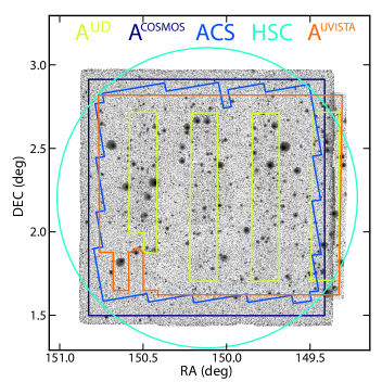
Figure 1.— Schematic of the COSMOS field showing all of the optical (dark blue and turquoise) and NIR (green and orange) observations used. The background image corresponds to the $\chi^{2}$ YKHK_s-z⁺⁺ detection image (as described in section 3). For reference, the region covered by the COSMOS-Advanced Camera for Surveys (ACS) HST data (Koekemoer et al., 2007) is shown in cyan. ${\cal A}^{\rm COSMOS}$ defines the 2 deg² COSMOS square (dark blue). ${\cal A}^{\rm Uvista}$ (orange area) is the region covered by the UltraVISTA-DR2 observations. We define ${\cal A}^{\rm UD}$ as the light green area, corresponding to the ultra-deep stripes in the UltraVISTA-DR2 observations. ${\cal A}^{\rm Deep}$ is the difference between ${\cal A}^{\rm UVista}$ and ${\cal A}^{\rm UD}$. In our analysis of the performance of the catalog, we limit ourselves to the intersection between ${\cal A}^{\rm UD}$ with ${\cal A}^{\rm COSMOS}$ and ${\cal A}^{\rm Deep}$ with ${\cal A}^{\rm COSMOS}$, after removing the masked objects in the optical bands (${\cal A}^{\rm!OPT}$, not shown on this figure). The effective areas are given in Table 7.

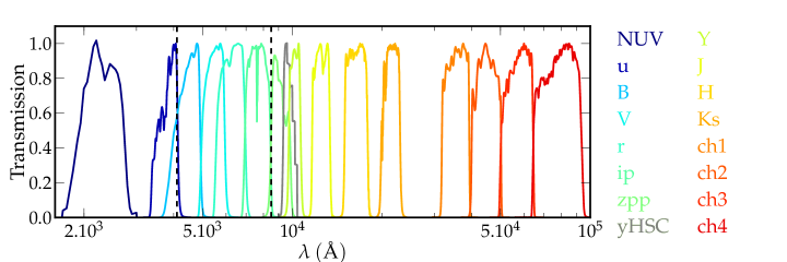
Figure 2.— Transmission curves for the photometric bands used. The effect of atmosphere, telescope, camera optics, filter, and the detector are included. Note that for clarity the profiles are normalized to a maximum throughput of one: therefore, the relative efficiencies of each telescope and detector system are not shown. Intermediate and narrow bands are not represented, but the region of the spectrum covered by these bands is marked by dashed lines.

Figure 3.— Limiting magnitude at 3$\sigma$ in a 3$\mathrm{\SIUnitSymbolArcsecond}$ diameter aperture computed from empty aperture measurements for each band in COSMOS2015, with the exception for NUV filter (value from Zamojski et al., 2007). The length of each segment is the FWHM of the filter curves. For the $Y$, $J$, $H$, $K_{\rm s}$ bands; the limiting magnitudes which are specified correspond to ${\cal A}^{\rm UD}$.

2.1.1 Optical-ultraviolet data

The optical-ultraviolet data set used here is similar to those used in previous releases (Capak et al., 2007; Ilbert et al., 2009). It includes near-UV ($0.23\mu m$) observations from GALEX (Zamojski et al., 2007), $u^{*}$-band data from the Canada-France Hawaii Telescope (CFHT/MegaCam), and the COSMOS-20 survey, which is composed of 6 broad bands ($B$, $V$, $g$, $r$, $i$, $z^{+}$), 12 medium bands ($IA427$, $IA464$, $IA484$, $IA505$, $IA527$, $IA574$, $IA624$, $IA679$, $IA709$, $IA738$, $IA767$, and $IA827$), and two narrow bands ($NB711$, $NB816$), taken with Subaru Suprime-Cam (Taniguchi et al., 2007, 2015). We have discarded poor seeing ($\sim 1.3\arcsec$) $g$-band data. Finally, the initial COSMOS $z$-band data were replaced by deeper $z^{++}$ band data taken with thinned upgraded CCDs and a slightly different filter. At this stage, in each band, image point-spread functions (PSFs) were homogenized to minimize tile-to-tile variations (Capak et al., 2007). At the same time, RMS_MAP and FLAG_MAP images were also generated, and saturated pixels and bad areas were flagged. This release also contains new $Y$-band data taken with Hyper-Suprime-Cam (HSC) Subaru (Miyazaki et al., 2012). The average exposure time per pixel is 2.1 hr. This data set is described fully in Hasinger G. et al. (in preparation). The addition of the $Y-$band data is intended to improve our stellar mass and redshift estimates in the important $1<z<1.5$ range because it is slightly bluer than the $Y$ filter from VIRCAM (see Figure 2), but it is also intended to serve as a “pilot program” to assess the utility of HSC data and to prepare for future COSMOS data sets which will include much more HSC imaging.

2.1.2 NIR data

The $YJHK_{\rm s}$-band data used here were taken between 2009 December 2009 and 2012 May with the VIRCAM instrument on the VISTA telescope as part of the UltraVISTA survey program and constitute the DR2 UltraVISTA release. The UltraVISTA-DR2 processing steps are the same as those in the DR1 release (McCracken et al., 2012). Compared to DR1, the exposure time has been increased significantly in the ultra-deep stripes, as shown in yellow in Figure 1; these cover an area of 0.62 deg². An important consequence of this is that the signal-to-noise ratio for an object of a given magnitude is not constant across the image. To provide NIR photometry in zones not covered by UltraVISTA, we include $H$ and $K$ WIRCAM data (McCracken et al., 2010) in our photometric catalog. However, this paper does not discuss the performance of photometric redshifts and physical parameters in these WIRCAM-only areas.

2.1.3 Mid-Infrared data

The $3.6\mu m$, $4.5\mu m$, $5.8\mu m$ and $8.0\mu m$ (respectively, channel 1, 2, 3, and 4) IRAC data used in this paper consist of the first two-thirds of the SPLASH COSMOS dataset together with S-COSMOS (Sanders et al., 2007), the Spitzer Extended Mission Deep Survey, the Spitzer-Candels survey data, along with a several smaller programs that observed the COSMOS field. The final processing is described in a companion paper (Capak et al. 2015 in prep). The average exposure time per pixel is 3.8 hr, increasing to 50hr in the central S-CANDELS coverage. Before processing, a median image was created for each AOR (observing block) and subtracted from the frames to remove residual bias in the frames and persistence from previous observations. For the S-CANDELS data, a secondary median was subtracted from the observations taken with repeats to remove the “first frame effect” residual bias. The resulting median-subtracted images have a mean background near zero, so no overlap correction was applied. The median subtracted frames were then combined with the MOPEX mosaic pipeline. The outlier and box-outlier modules were used to reject cosmic rays, transients, and moving objects. The data were then drizzled onto a $0.6\arcsec$ pixel scale using a “pixfrac” of 0.65 and combined with an exposure time weighted mean combination. Mean, median, coverage, uncertainty, standard-deviation, and color-term mosaics were also created. Obviously, this variation as a function of position can be expected to have an influence on the precision of the photometric redshifts and stellar masses for the very highest redshift ($z>4$) objects.

Table 1Summary of available data in each band and the average limiting magnitudes computed from variance map in 2 and 3$\mathrm{\SIUnitSymbolArcsecond}$ diameter apertures on the PSF-homogenised Images. The central wavelength is the median wavelength weighted by transmission and the widths are defined using the half-maximum transmission points.

Instrument	Filter	Central	Width	3$\sigma$ depth a
/Telescope		$\lambda$ ($\mathrm{\SIUnitSymbolAngstrom}$)	($\mathrm{\SIUnitSymbolAngstrom}$)	(3$\mathrm{\SIUnitSymbolArcsecond}$/2$\mathrm{\SIUnitSymbolArcsecond}$)
(Survey)				$\pm 0.1$
GALEX	NUV	2313.9	748	25.5 b
MegaCam/CFHT	$u^{*}$	3823.3	670	26.6/ 27.2
Suprime-Cam	$B$	4458.3	946	27.0/ 27.6
/Subaru	$V$	5477.8	955	26.2/ 26.9
	$r$	6288.7	1382	26.5/ 27.0
	$i^{+}$	7683.9	1497	26.2/ 26.9
	$z^{++}$	9105.7	1370	25.9/ 26.4
	$IA427$	4263.4	206.5	25.9/ 26.5
	$IA464$	4635.1	218.0	25.9 / 26.5
	$IA484$	4849.2	228.5	25.9/ 26.5
	$IA505$	5062.5	230.5	25.7/ 26.2
	$IA527$	5261.1	242.0	26.1/ 26.6
	$IA574$	5764.8	271.5	25.5/ 26.0
	$IA624$	6233.1	300.5	25.9/ 26.4
	$IA679$	6781.1	336.0	25.4/ 26.0
	$IA709$	7073.6	315.5	25.7/ 26.2
	$IA738$	7361.6	323.5	25.6/ 26.1
	$IA767$	7684.9	364.0	25.3/ 25.8
	$IA827$	8244.5	343.5	25.2/ 25.8
	$NB711$	7119.9	72.5	25.1/ 25.7
	$NB816$	8149.4	119.5	25.2/ 25.8
HSC/Subaru	$Y$	9791.4	820	24.4/ 24.9
VIRCAM	$Y^{\rm UD}$	10214.2	970	25.3/ 25.8
/VISTA	$Y^{\rm Deep}$			24.8/ 25.3
(UltraVISTA-DR2)	$J^{\rm UD}$	12534.6	1720	24.9/ 25.4
	$J^{\rm Deep}$			24.7/ 25.2
	$H^{\rm UD}$	16453.4	2900	24.6/ 25.0
	$H^{\rm Deep}$			24.3/ 24.9
	$K_{\rm s}^{\rm UD}$	21539.9	3090	24.7/25.2
	$K_{\rm s}^{\rm Deep}$			24.0/ 24.5
WIRCam	$K_{\rm s}$	21590.4	3120	23.4/ 23.9
/CFHT	$H$	16311.4	3000	23.5/ 24.1
IRAC/Spitzer	ch1	35634.3	7460	25.5/ o c
(SPLASH)	ch2	45110.1	10110	25.5/ oc
	ch3	57593.4	14140	23.0/ oc
	ch4	79594.9	28760	22.9/ o c

• $3\sigma$ depth in $m_{\rm AB}$ computed on PSF-matched images from around 800 apertures at 2 and 3$\mathrm{\SIUnitSymbolArcsecond}$.

• Value given in Zamojski et al. (2007) corresponding to a 3$\sigma$ depth.

• $3\sigma$ depth in $m_{\rm AB}$ computed from the RMS maps, after masking the area containing an objects based on the segmentation map.

2.2. Image Homogenisation

In this paper, the variation of the PSF across individual images in a given band is neglected. This is reasonable because band-to-band variations are almost always greater than the variation within a single band. The residual impact of the PSF variation across the field is discussed in Appendix 7.3.

From $u$ to $K_{\rm s}$ the FWHM of the PSF has a range of values between $\sim 0.5\mathrm{\SIUnitSymbolArcsecond}$ and $1.02\mathrm{\SIUnitSymbolArcsecond}$ (corresponding to a Moffat fit). Therefore, the fraction of the total flux falling in a fixed aperture is band-dependent. One way to address this problem is to “homogenize” the PSF so that it is the same in all of the bands (GALEX and IRAC bands are not homogenized, their photometry are extracted with a source-fitting technique, as detailed in section 3). In the first step in our homogenization process, SExtractor (Bertin & Arnouts, 1996) is used to extract a catalog of bright objects. Stars are identified by cross-matching with point sources in the COSMOS-Advanced Camera for Surveys (ACS) Hubble Space Telescope (HST) catalog (Koekemoer et al., 2007; Leauthaud et al., 2007). Saturated or faint stars are removed by considering the position of each object in the FWHM versus m_AB diagram. For each star we extract a postage stamp using SExtractor.

The PSF is modelled in pixel space using PSFex (Bertin, 2013) as a linear combination of a limited number of known basis functions:

$$\Psi_{c}=\sum_{b}c_{b}\psi_{b}$$ (1)

where the $c$ index reflects the dependance of $\Psi$ on the set of coefficients $c_{b}$. Given a basis, this PSF model can be entirely determined knowing the coefficients $c_{b}$ of the linear combination. The pixel basis is the most “natural” basis but requires as many coefficients as the number of pixels on the image postage stamp. We can then make some assumptions to simplify the basis and to reduce the number of coefficients. The adopted basis is the “polar shapelet” basis (Massey & Refregier, 2005), for which the components have useful explicit rotational symmetries. We assume that the PSF is constant over the field. The global PSF of one band is then expressed as a function of the coefficients $c_{b}$ at each pixel position $x_{i}$ on the postage stamp image, which are derived by minimizing the $\chi^{2}$ sum over all of the sources:

$$\chi^{2}(c)=\sum_{{\rm sources}\,s}\sum_{{\rm pixels}\,i}\frac{(p_{s}(x_{i})-f_{s}\Psi_{c}(x_{i}))^{2}}{\sigma_{i}^{2}},$$ (2)

where $f_{s}$ is the total flux of the source $s$, $\sigma_{i}$ is the variance estimate of pixel $i$ of the source $s$, $p_{s}(x_{i})$ is the intensity of the pixel $i$, and $c$ refers to the set of PSF coefficients. Once the global PSF has been determined in each band, we then decide on the “target PSF”, corresponding to the desired PSF of all of the bands after homogenization. This is chosen so as to minimize the applied convolutions. We use a Moffat profile to represent the PSF (Moffat, 1969); this provides a better description of the inner and outer regions of the profile than a simple Gaussian. The stellar radial light profile is

$$I_{r}=I_{0}[1+(r/\alpha)^{2}]^{-\beta}$$ (3)

with $\alpha={\theta}/(2\sqrt{2^{1/\beta}-1}),$ $I_{0}=(\beta-1)(\pi\alpha^{2})^{-1}$ and $\theta$ the FWHM. Our target PSF is defined as a Moffat profile with ${\cal M}\left[\theta,\beta\right]={\cal M}\left[0.8\mathrm{\SIUnitSymbolArcsecond},2.5\right].$

The required convolution kernel is calculated in each band by finding the kernel that minimizes the difference between the target PSF and the convolution product of this kernel with the current PSF. The images are then convolved with this kernel.

To estimate the precision of our PSF matching procedure, the photometry of the stars is extracted at 14 fixed apertures of radii $r_{k}$, logarithmically spaced between 0.25$\mathrm{\SIUnitSymbolArcsecond}$ and 2.5$\mathrm{\SIUnitSymbolArcsecond}$. In each band, the difference between the magnitude of the stars extracted in the aperture $r_{k}$ and the total magnitude (computed from the 4$\arcsec$ diameter aperture) is plotted in Figure 4 as a function of aperture. For comparison, the difference that would be obtained with the target profile ${\cal M}\left[0.8\mathrm{\SIUnitSymbolArcsecond},2.5\right]$ is overplotted as a red dashed line. The agreement is excellent up to a 2$\mathrm{\SIUnitSymbolArcsecond}$ radius on the plot.

The flux obtained with the best-fitting PSF in each band is normalized to the target profile and also plotted in Figure 4 (left panel), before and after homogenization. For perfect homogenization, this ratio should be one, independent of aperture. For the 3$\mathrm{\SIUnitSymbolArcsecond}$ diameter aperture, the relative photometric error for point-sources objects after homogenization is below $5\%$ (or equivalently a difference of $\sim$0.05 in magnitude). Unfortunately, despite previous attempts at PSF homogenization inside each field (Capak et al., 2007; McCracken et al., 2012), residual variations remain across the field. These are shown in Figure 5, which shows the distribution of the stellar FWHM and the median FWHM for two representative bands. While the PSF is relatively homogenous across the field for most of the bands (e.g $u$-band),there is larger scatter for some bands (e.g $IA464$). In Appendix 7.3, we discuss the effect of these variations on the aperture magnitude.

Concerning the cosmetic quality of the image, the convolution operation produces several undesirable effects. First, it induces a covariance in the background noise which can lead photometric errors being underestimated. Secondly, since the homogenization process acts both on the FWHM and the profile slope ($\alpha$ and $\beta$ parameters), the convolution kernel may contains negative components. In some bands it can lead to artefacts (such as rings) around saturated objects. We mask these saturated objects in the final catalog. We deal with the correlation of the background by multiplying in each band the photometric errors derived from SExtractor by a correction factor (see section 3.2 for more details).

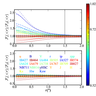
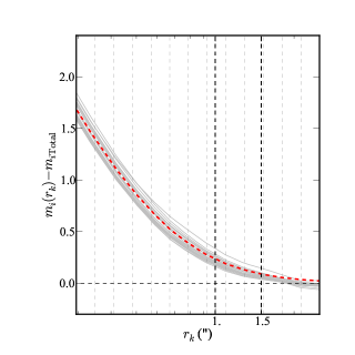
Figure 4.— Left: best-fitting stellar PSFs for all bands before and after homogenization (left upper and lower panels respectively), normalized to the target PSF ${\cal F}_{T}$. The vertical black solid line corresponds to the 3$\arcsec$ diameter aperture used for photometric redshifts. The horizontal dashed lines show the 5% relative error. The color map reflects the increase in seeing before homogenization. Right: Median curves of growth (the difference between the magnitude in the $k$th aperture $r_{k}$ with the total magnitude for point-like sources, estimated from the 4$\arcsec$ diameter aperture) as a function of aperture after homogenization for each band. The target Moffat profile with ($\theta$,$\beta$)=(0.8,2.5) is shown in red. The vertical dark dashed lines are the apertures provided in the final public catalog (2$\mathrm{\SIUnitSymbolArcsecond}$ and 3$\mathrm{\SIUnitSymbolArcsecond}$ diameters).

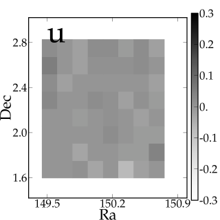
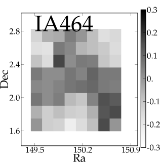
Figure 5.— Distribution of the difference local seeing and the median image seeing for the selected stars in the $u$ and $IA464$ bands as a function of the position. Note that for these seeing estimations, we did not fit each star individually with a Moffat profile, but we used the Gaussian-profile-based FWHM_WORLD parameter from SExtractor. While the $u$ band is relatively homogenous across the field, $IA464$ shows large positional variations. This is the most extreme case in our catalog.

3. Catalog extraction

3.1. Photometric measurements

3.1.1 Optical and NIR data

Object photometry is carried out using SExtractor in “dual image” mode. The $\chi^{2}$ $zYJHK_{\rm s}$ detection image (Szalay et al., 1999) is produced using SWarp (Bertin et al., 2002) starting with the non-homogenized images. Since the main objective of our new catalog is to probe the high-redshift Universe and also to provide a catalog containing UV-luminous sources at $z>2$, we create a detection image by combining NIR images of UltraVISTA ($YJHK_{\rm s}$) with the optical $z^{++}$-band data from Subaru. We do not use $i^{+}$-band data since compact objects in the $i^{+}$ image saturate around $i=21$.

We extract fluxes from 2 and 3$\mathrm{\SIUnitSymbolArcsecond}$ diameter apertures on PSF-homogenized images in each band. The well-known difficulty in source extraction from astronomical images is that objects have ill-defined, potentially overlapping boundaries, making flux measurements challenging. The two main parameters that control extraction are the deblending threshold and the flux threshold. Therefore, a reasonable balance must be found on one hand between deblending too much (splitting objects) and not deblending enough (leading to merging). Simliar problems occur with the choice of the detection threshold: a low detection threshold can create too many spurious objects, and one that is too high may miss objects. This can be mitigated in part by a judicious choice of detection threshold and the minimal number of contiguous pixels which constitute an object. The solution we adopt is to set a low deblending and detection threshold while increasing the number of contiguous pixels to reject false detections. We validated this choice through careful inspection of catalogs superimposed on the detection and measurement images, which is feasible in the case of a single-field survey like COSMOS.

The background is estimated locally within a rectangular annulus (30 pixels thick) around the objects, delimited by their isophotal limits. Additionally, object mask flags indicating bad regions in the optical and NIR bands were included and saturated pixels in the optical bands were flagged by using the appropriate FLAG_MAPs. Our chosen parameters are given in Table 9.

In the last step, catalogs from each band are merged together into a single FITS table and galactic extinction values are computed at each object position using the Schlegel et al. (1998) values. These reddening values have to be multiplied by a factor computed for each band, derived from the filter response function and integrated against the galactic extinction curve (Bolzonella et al., 2000; Allen, 1976). These factors are shown in Table 3.

3.1.2 GALEX photometry

As in Ilbert et al. (2009), GALEX photometry (Zamojski et al., 2007) for each object was derived by cross-matching our catalog with the publicly available photometric $i^{+}$-selected catalog described in Capak et al. (2007). GALEX fluxes were measured using a PSF fitting method with the $u^{*}$-band image used as a prior.

3.1.3 IRAC photometry

The SPLASH data exceed the confusion limits in IRAC channel 1 and channel 2; better deblending techniques are necessary to estimate fluxes in these crowded, low-resolution images. We use IRACLEAN (Hsieh et al., 2012) to derive the SPLASH photometry.This makes use of the positional and morphological characteristics of objects detected in a high-resolution image in a different waveband to deblend objects and derive more accurate fluxes in low-resolution images. Unlike other similar methods assuming that the intrinsic morphology of an object is identical in the two wavebands (i.e., there is no morphological k-correction), IRACLEAN is essentially the same as CLEAN deconvolution in radio imaging with nearly no morphological restrictions, except for the locations where CLEAN can opperate. This scheme minimizes the effect of morphological k-correction when a high-resolution image (i.e., the prior) and its low-resolution counterpart are taken in very different wavebands. However, there is a limitation for this scheme. If the separation of two objects is less than $\sim 1$ FWHM, then the flux of the brighter object can be overestimated while the flux of the fainter one can be underestimated, as discussed in Hsieh et al. (2012). To solve this issue, we improve IRACLEAN by taking the surface brightness information in the prior into account. The new IRACLEAN uses the surface brightness of the prior to weight where CLEAN occurs for each object. The weighting strength is determined by the power of the surface brightness, i.e., (surface brightness of the prior)ⁿ, where $n$ is the weighting parameter. If $n$ is zero, then the surface brightness of the prior is ignored, and so the new IRACLEAN behaves like the original IRACLEAN. When $n$ is greater than zero, the higher the $n$ is, the more heavily weighted the surface brightness is. If the wavebands of the prior and the target images are very different, then $n$ can be set to a lower value, e.g., 0.1 - 0.3.If the wavebands of the prior and the target images are very similar, then $n$ can be set to a higher value, e.g., 0.3 - 0.5. In general, $n=0.3$ is sufficiently good for most cases.

In this paper, the UltraVISTA $zYJHK_{\rm s}$ chi-square image is used as the prior for the SPLASH images in IRACLEAN. To accelerate the process, both the UltraVISTA $zYJHK_{\rm s}$ chi-square image and the SPLASH images are broken up into the 144 tiles that are used for the COSMOS Subaru/ACS data, making parallel processing easier. The tiles overlap by 14.4$\mathrm{\SIUnitSymbolArcsecond}$ around the edges to avoid flux underestimation for those objects close to the edges of the tiles. The SPLASH PSFs in each tile are generated using point sources in that tile. The aperture size used to measure the flux ratios between sources and PSFs for the CLEAN procedure is $1.8\mathrm{\SIUnitSymbolArcsecond}\times 1.8\mathrm{\SIUnitSymbolArcsecond}$, and the weighting parameter n is 0.3. After the CLEAN procedure is completed, a residual map is generated which is used toe stimate the flux errors. The flux error of each object is estimated based on the fluctuations in the local area around that object in the residual map. The IRACLEAN procedure is described fully in Hsieh et al. (2012).

3.1.4 X-ray photometry

The Chandra COSMOS-Legacy Survey (Civano et al., 2016; Marchesi et al., 2016) contains 4016 X-ray sources down to a flux limit of $f_{X}\simeq$2 $\times$ 10^-16 erg s^-1 cm^-2 in the 0.5-2 keV band: 3755 of these sources lie inside the UltraVISTA field of view. The Chandra COSMOS-Legacy catalog was matched with the UltraVISTA catalog using the Likelihood Ratio (LR) ratio technique (Sutherland & Saunders, 1992). This method provides a much more statistically accurate result than a simple positional match, taking into account the following: (i) the separation between the X-ray source and the candidate UltraVISTA counterpart; (ii) the counterpart $K$-band magnitude with respect to the overall magnitude distribution of sources in the field. Of the 3755 Chandra COSMOS-Legacy sources, 3459 ($\simeq$92%) have an UltraVISTA counterpart. In the catalog we also added the match with X-ray detected sources from XMM-COSMOS (Hasinger et al., 2007; Cappelluti et al., 2007; Brusa et al., 2010) and the previous Chandra COSMOS catalog (Elvis et al., 2009; Civano et al., 2012).

3.1.5 Far-IR photometry

Photometry at 24$\mu$m was obtained for a total of 42633 sources using an updated version of the COSMOS MIPS-selected band-merged catalog published by Le Floc’h et al. (2009). In this catalog,  90% of the 24$\mu$m-selected sources were securely matched to their $K_{\rm s}$-band counterpart using the WIRCAM COSMOS map of McCracken et al. (2010), assuming a matching radius of 2 $\arcsec$. Counterparts to another 5% of the sample were found using the IRAC-3.6$\mu$m COSMOS catalog of Sanders et al. (2007), while the rest of the 24$\mu$m source population remained unidentified at shorter wavelengths. We thus considered the coordinates of the WIRCAM K-band or IRAC counterparts (or the initial 24$\mu$m coordinates for the unidentified MIPS sources), and cross-correlated these positions with the VISTA catalog using a matching radius of 1$\arcsec$. VISTA counterparts were found for all of the previously-identified 24$\mu$m sources and for an additional set of 117 objects detected by MIPS which had no previous identification.

We also provide Far-IR photometry obtained at 100, 160, 250, 350, and 500$\mu$m using the PACS (Poglitsch et al., 2010) and SPIRE (Griffin et al., 2010) observations of the COSMOS field with the Herschel Space Observatory. The PACS data were obtained as part of the PEP guaranteed time program (Lutz et al., 2011), while the SPIRE observations were carried out by the HERMES consortium (Oliver et al., 2012). For each band observed with Herschel, source extraction was performed by a PSF fitting algorithm and using the 24$\mu$m source catalog as priors. Hence, far-IR matches to VISTA were unambiguously obtained from the 24$\mu$m source counterparts described above, leading to a total of 6608 sources with a PACS detection and 17923 sources detected with SPIRE. Total uncertainties in the SPIRE bands include the contribution from confusion. Flux density measurements with a signal to noise smaller than 3 in the initial SPIRE COSMOS catalog published by Oliver et al. (2012) are not considered in our present work.

3.2. Computation of photometric errors and upper limits

Precise photometric error measurements are essential for accurate photometric redshifts. For each Subaru band, we use effective gain values (Capak et al., 2007) for the non-convolved data to compute the magnitude errors. This is particularly important for the Subaru bands because of the long exposure times used for each individual exposure. However, because SExtractor errors are underestimated in data with correlated noise, we multiply the magnitude and flux errors with a correction factor computed for each band from empty apertures (based on the segmentation map, apertures that contain an object have been discarded). Following Bielby et al. (2012), this factor is computed in each band for the 2 and 3$\arcsec$ apertures and taken at the ratio between the standard deviation of the flux extracted in empty apertures on the field and the median of the SExtractor errors. For UltraVISTA, we compute separate values for the Ultra-deep (${\cal A}^{\rm UD}$) and deep (${\cal A}^{\rm Deep}$) regions. The corrections are given in Table 3.

In some bands, a source may be below the measurement threshold while at the same time be detected in the combined $zYJHK_{\rm s}$ $\chi^{2}$ image. In this case, in the measurement band, SExtractor may not report consistent magnitudes or magnitude errors, and we report upper limits on the source magnitudes in each band where they are too faint to be detected. To compute the magnitude limits, we run SExtractor on each individual image using the same detection parameters. All of the pixels belonging to objects are flagged. Fluxes are measured from PSF-homogenized images in empty apertures of 2 and $3\mathrm{\SIUnitSymbolArcsecond}$, discarding all of the apertures containing an object. The magnitude limit is then computed from the standard deviation of fluxes in each aperture.

This method is not always appropriate since the values of the upper limits may vary over the field, as shown in Figure 6. This is why we use a local estimate for the upper limits in the six broad bands of optical data ($u$, $B$, $V$, $r$, $i^{+}$, $z^{++}$). In these bands, upper limits are calculated for each object from the variance map and are defined as being the square root of the variance per pixel integrated over the aperture. The magnitude of the object is set to the 3$\sigma$ magnitude limit if the flux is below the 3$\sigma$ flux limit, or if the flux is below the flux error. The averaged values of these upper limits are consistent with the value computed with the first method and are displayed in Table 1. The upper limits in these bands are important because young, star-forming objects at high redshift will have apparent magnitudes in the optical bands of the order of the limiting magnitude. The computation of the photometric redshift uses fluxes and so does not use the upper limits which are only applied to the magnitudes, but it may be useful when working with magnitudes to know whether or not the object is within the upper limit.

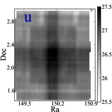
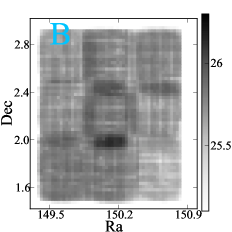
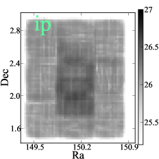
Figure 6.— The locally computed magnitude limits computed from the variance map as a function of right ascension and declination for $u$, $B$ and $i^{+}$ bands in a 2$\arcsec$ diameter aperture.

3.3. Catalog validation

3.3.1 Number counts

In Figure 7, we plot the number of galaxies per square degree per magnitude as a function of $K_{\rm s}$ magnitude for objects in both the ${\cal A}^{\rm Deep}$ and ${\cal A}^{\rm UD}$ regions (details of the stars-galaxy separations can be found in Section 4.5). The corresponding values are presented in Table 2.

Our counts are in excellent agreement with the literature. We reach more than one magnitude deeper compared to the previous UltraVISTA-DR1 (McCracken et al., 2012). In addition, our counts are in good agreement with the much deeper Hawk-I survey (Fontana et al., 2014) up to at least $K_{\rm s}\sim 24.5$.

At the $3\sigma$ limit in $K_{\rm s}$, we detect almost twice as many objects per square degree in ${\cal A}^{\rm UD}$ than in ${\cal A}^{\rm Deep}$. Furthermore, our catalog contains $\sim 1.5\times 10^{5}$ objects with $K_{\rm s}<24.7$ in the ${\cal A}^{\rm UD}$ compared to $\sim 0.8\times 10^{5}$ found with UltraVista-DR1 (McCracken et al., 2012) in the same region at the detection limit in $K_{\rm s}$. In ${\cal A}^{\rm Deep}$, the difference is less significant since the depths are comparable, with $\sim 0.9\times 10^{5}$ objects compared to $\sim 0.7\times 10^{5}$ found in UltraVista-DR1.

Compared with the previous publicly available photometric $i^{+}$-selected catalog (described in footnote 4) at the detection limit $i^{+}<26.1$ (limiting magnitude at 5$\sigma$ in a 3 $\arcsec$ diameter aperture from Capak et al., 2007), we find that 16.1% of sources are not present in COSMOS2015, as shown on figure 8. Many of these missing sources are blue, faint ($25.5<i^{+}<26.1$), low-mass, star forming galaxies. This difference is to be expected, since an NIR-only selection and a pure $i^{+}$-selection are not expected to sample the same galaxy populations. However, we have mitigated this difference by including the $z^{++}$ band in our detection image; this percentage is smaller than in Ilbert et al. (2013), where the detection image was shallower and did not include any optical bands. Furthermore, the previous $i^{+}$-selected catalog also contained spurious objects near the detection limit, and therefore the fraction of missed genuine objects can be expected to be lower.

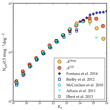
Figure 7.— $K_{\rm s}$-band-selected galaxy number counts of the $YJHK_{\rm s}z^{++}$-detected galaxies in ${\cal A}^{\rm UD}$ (yellow circles) and ${\cal A}^{\rm Deep}$ (pink circles), compared to a selection of literature measurements. The Ilbert et al. (2013) and McCracken et al. (2010) points show previous measurements in COSMOS.

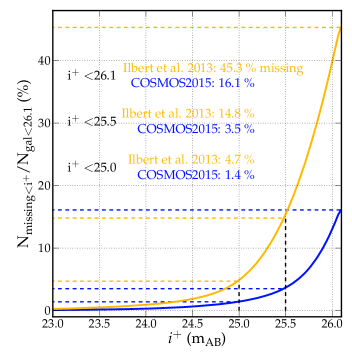
Figure 8.— Cumulative distribution of the number of galaxies over the total number of galaxies in a magnitude-limited sample ($i^{+}<26.1$) as a function of magnitude in the $i^{+}$-band from Capak et al. (2007) which are not recovered in Ilbert et al. (2013) (orange line) and this catalog (blue line).

Table 2$K_{\rm s}$-band-selected galaxy number counts. Logarithmic galaxy number counts are in units of galaxies per 0.5 magnitude per square degree.

Magnitude Bin	Deep Regions	Ultra-Deep Regions
		regions
$\left[16.0-16.5\right]$	2.24	2.19
$\left[16.5-17.0\right]$	2.28	2.33
$\left[17.0-17.5\right]$	2.58	2.60
$\left[17.5-18.0\right]$	2.72	2.80
$\left[18.0-18.5\right]$	2.94	3.00
$\left[18.5-19.0\right]$	3.19	3.24
$\left[19.0-19.5\right]$	3.39	3.42
$\left[19.5-20.0\right]$	3.57	3.62
$\left[20.0-20.5\right]$	3.73	3.76
$\left[20.5-21.0\right]$	3.87	3.89
$\left[21.0-21.5\right]$	3.99	4.01
$\left[21.5-22.0\right]$	4.11	4.14
$\left[22.0-22.5\right]$	4.23	4.23
$\left[22.5-23.0\right]$	4.35	4.36
$\left[23.0-23.5\right]$	4.48	4.46
$\left[23.5-24.0\right]$	4.59	4.55
$\left[24.0-24.5\right]$	4.65	4.64
$\left[24.5-25.0\right]$	4.63	4.69
$\left[25.0-25.5\right]$	4.49	4.68
$\left[25.5-26.0\right]$	4.27	4.54

3.3.2 Astrometric accuracy

We compared the astrometric positions of bright, non-saturated objects in COSMOS2015 with those in the COSMOS reference catalog from Leauthaud et al. (2007) and the publicly available $i^{+}$-selected photometric catalog (footnote 4) described in Capak et al. (2007). This is illustrated in Figure 9. There is good agreement between COSMOS2015 and the Leauthaud et al. (2007) catalog. The shift between the $i^{+}$-selected catalog and Leauthaud et al. (2007) is no longer present in COSMOS2015. This shift occurs below a pixel size of 0.15$\arcsec$. These comparisons show that our astrometry is accurate to at least one pixel.

We note that the COSMOS astrometric reference catalog used in McCracken et al. (2010, 2012) and this paper is based on a reference catalog extracted from a Megacam $i$-band (data taken in 2004) image covering the full COSMOS field. The astrometric zero point of this catalog was set using radio interferometric observations (Schinnerer et al., 2004). Until now, at scale smaller than the size of the resampled pixels, it has been challenging to test the astrometric accuracy for our catalog given the lack of availability of sufficiently dense astrometric catalogs. However, we have compared the positions between our catalog and the catalogs extracted from the independently reduced Hyper Suprime-Cam images described here, and this has confirmed that our astrometric solutions are good at the level of one pixel. For future data releases, we intend to improve our overall astrometric precision by using densely sampled catalogs based on either Hyper Suprime-Cam or Pann-Starrs data, which are tied to 2MASS.

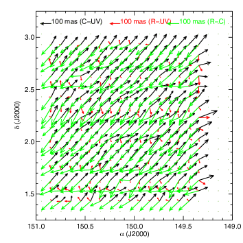
Figure 9.— Astrometric comparison for bright objects between our catalog, the catalog from Leauthaud et al. (2007) and the publicly available COSMOS $i^{+}$-selected catalog (Capak et al., 2007). Black arrows show the shift between Capak et al. and COSMOS2015, red arrows between Leauthaud et al. (2007) and COSMOS2015. Finally, green arrows show the shift between the two previous catalogs. All of these shifts occur below one pixel.

4. Photometric Redshift and physical parameters

4.1. Input catalog

We use fluxes rather than magnitudes for our photometric measurements to deal robustly with faint or non-detected objects. Faint objects may have a physically meaningful flux measurement, whereas their magnitudes and magnitude errors may be undetermined (for example, if the flux is negative). Consequently, when using magnitudes, we must set an upper limit: for flux measurements with correct flux errors, this is no longer necessary. There is no loss of information when using flux measurements. This leads to a better determination of the photometric redshift and a lower number of catastrophic failures at $z>2$.

Photometric redshifts are computed using 3$\arcsec$ aperture fluxes. The fixed-aperture magnitude estimate is expected to be less noisy for faint sources than the pseudo-total Kron (Kron, 1980) magnitudes mag_auto. This is because mag_auto’s variable aperture is derived from the detection image, which means that fainter objects have can potentially have noisier colors (Hildebrandt et al., 2012; Moutard et al., 2016). This magnitude measurement is also susceptible to blended sources. We find that the 3$\arcsec$ aperture photometry gives slightly better photometric redshifts than the 2$\arcsec$ aperture at low redshift (below $z\leq 1$) and we adopt this aperture over the entire redshift range of our survey. We suspect that the photometric redshift precision is lower in the 2$\arcsec$ apertures due to small-scale residual astrometric errors. This is being investigated for the upcoming DR3 UltraVISTA release.

Photometric redshift computations use colors, and, consequently, should not be sensitive to a systematic magnitude calibration offset. However, in contrast to optical and NIR data, GALEX and IRAC data provide total magnitudes or fluxes, which require an estimate of the total flux from the corrected 3$\mathrm{\SIUnitSymbolArcsecond}$ aperture fluxes to be consistent over the full wavelength range. This is also needed to derive stellar masses. For each object, we compute a single offset $o$ (the same for all the bands) which allows for the conversion from aperture to total magnitude. The offset is computed following Moutard et al. (2016):

$$o= \frac{1}{\sum_{\rm filters\,i}{\rm w}_{i}}\times$$ (4)

$$\sum_{\rm filters\,i}\left({\rm MAG}_{\rm AUTO}-{\rm MAG}_{\rm APER}\right)_{i}\times{\rm w}_{i}$$

where we have:

$${\rm w}_{i}=\frac{1}{\left({\sigma}^{2}_{\rm AUTO}+{\sigma}^{2}_{\rm APER}\right)_{i}}$$ (5)

This leads to the assumption that the PSF profile is the same in all of the bands. As it is averaged over all of the broad bands, i.e, $u$, $B$, $V$, $r$, $i^{+}$, $z^{++}$, $Y$, $J$, $H$, and $K_{\rm s}$, this offset is more robust than the one which would have been computed by band. These offsets are given in the final catalog.

4.2. Method

To compute the photometric redshifts, we use LePhare (Arnouts et al., 2002; Ilbert et al., 2006) with the same method as used in Ilbert et al. (2013). Our aim is to compute precise photometric redshifts over a wide redshift range and for many object types with minimum bias. Obviously, a single set of recipes will not perform as well as several configurations, with each one tuned to optimize the fit at different redshifts. That is why we use a set of 31 templates including spiral and elliptical galaxies from Polletta et al. (2007) and a set of 12 templates of young blue star-forming galaxies using Bruzual & Charlot (2003) models (BC03). Extinction is added as a free parameter ($E(B-V)<0.5$) and several extinction laws are considered: those of Calzetti et al. (2000), Prevot et al. (1984) and a modified version of the Calzetti laws including a “bump” at 2175Å (Fitzpatrick & Massa, 1986). Using a spectroscopic sample of quiescent galaxies, Onodera et al. (2012) showed that the estimate of the photometric redshift for the quiescent galaxies in Ilbert et al. (2009) were underestimated at $1.5<z<2$. Following Ilbert et al. (2013), we improved the photometric redshift for this specific population by adding two new BC03 templates assuming an exponentially declining SFR with a short timescale $\tau=0.3\,\mathrm{Gyr}$ and extinction-free templates.

Finally, we compute the predicted fluxes in every band for each template and following a redshift grid with a step of 0.01 and a maximum redshift of 6. The computation of the fluxes also takes into account the contribution of emission lines using an empirical relation between the UV light and the emission line fluxes as described in Ilbert et al. (2009).

The code performs the $\chi^{2}$ analysis between the fluxes predicted by the templates and the observed fluxes of each galaxy. At each redshift, $z_{\rm step}$, and for each template of the library, the $\chi^{2}$ is computed as

$$\chi^{2}(z_{\rm step})=\sum_{\rm filters\,i}\frac{(F_{\rm obs\,i}-\alpha F_{\rm SED\,i}(z_{\rm step},T))^{2}}{\sigma^{2}_{\rm obs\,i}}$$ (6)

where $F_{\rm SED\,i}(z_{\rm step},T)$ is the flux predicted for a template $T$ at $z_{\rm step}$ and $\alpha$ is the normalization factor. Then, the $\chi^{2}$ is converted to a probability of $p=\exp^{-\chi^{2}/2}$. All of the probability values are summed up at each redshift $z_{\rm step}$ to produce the Probability Distribution Function (PDF). We then determine then the photometric redshift solution from the median of this distribution. The 1$\sigma$ uncertainties given in the catalog are derived directly from the PDF and enclose 68% of the area around the median.

An important aspect of the method is the computation of systematic offsets which are applied to match the predicted magnitudes and the observed ones (Ilbert et al., 2006). We measure these offsets using the spectroscopic sample. For each object, we search for the template which minimizes the $\chi^{2}$ at fixed redshift. Then, we measure the systematic offset which minimizes the difference between the predicted and observed magnitudes. This procedure iterates until convergence.

The photometric redshift distribution for the $i^{+}$- and $K_{\rm s}$-selected samples is given in Figure 10. Magnitudes are measured in corrected 3” aperture magnitudes with the derived systematic offset applied. Several interesting trends are apparent. In general, the median redshift of our $K_{\rm s}-$ sample is higher than our $i^{+}$-selected samples. Also, the fraction of sources at higher redshifts is greater for the NIR-selected samples. These effects are largely due to the well-known positive evolutionary corrections and $k-$ corrections for NIR-selected samples. Optically selected samples at higher redshifts move progressively to shorter rest-frame UV wavelengths, which are strongly attenuated by dust and the intergalactic medium. We compare these distributions with a simple three-components galaxy population model generated with the PEGASE.2 code (Fioc & Rocca-Volmerange, 1997, 1999). Each population starts forming at $z=8$ via the infall of pristine gas on a specific timescale and gas is converted into stars at a specific rate. The corresponding star formation histories peak at $z\sim 4$, 2 and 0, and the $z=0$ predicted optical-NIR colors correspond to those of local Sa, Sbc, and Sd galaxies, respectively. The total baryonic mass (gas, stars, and hot halo-gas) of each galaxy is assumed to be constant, and the mass function of each population is tuned so that the sum of the three populations matches simultaneously the local luminosity function in the $B$ band, the deep galaxy counts in the $B$, $V$, $I$, and $K_{\rm s}$ band, as well as the cosmic star formation rate density and the stellar mass density observed at $z=0-6$. The agreement between the data and this simple three-component model is quite good. This success lies in the differential contributions of the three galaxy populations to the counts. Indeed, our modeled counts at $K_{\rm s}=24$ are the sums of the almost equal contributions of Sd progenitors at $z\sim$0.7, of Sb progenitors at $z\sim$1.2, and Sab progenitors at $z\sim$2. In contrast, a simpler modeling of the galaxy populations using a single scenario with an SFH proportional to SFRD($z$) (Star Formation Rate Density) and a unique mass function leads to very good agreement between the integrated counts in $i^{+}$ and $K_{\rm s}$ bands, as well as a good match between the SFRD($z$) and $\rho_{*}(z)$, but it completely overshoots the mean redshift of the $K_{\rm s}\sim$24 or $i^{+}\sim$24.5 sources ($z\sim$2, whereas the COSMOS data shows it is peaked at $z\leq$1). Other choices of modeling that we explored also lead to a high level of tension either in the SFRD($z$), $\rho_{*}(z)$ or in the counts in the $i^{+}$, $K_{\rm s}$ or $B$ bands.

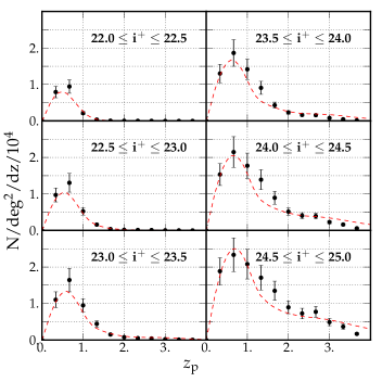
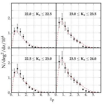
Figure 10.— Photometric redshift distributions for $i^{+}-$ (left) and $K_{\rm s}$(right)-selected samples for the full sample, compared with a model prediction (red dashed line) from PEGASE.2 (Fioc & Rocca-Volmerange, 1997, 1999). Plotted errorbars are uncertainties estimated from jacknife errors, splitting the field into 25 sub-fields.

Table 3Photometric corrections, including multiplicative error factors for SExtractor (see Section 3.2), systematic offsets ($s_{f}$) derived from the spectroscopic sample (see Section 4.2) and factors $F$ for the foreground extinction (Allen, 1976). $s_{f}$ values have to be subtracted to the apparent magnitudes.

	band	error	error	$s_{f}$	$F$
		fact. (2$\arcsec$)	fact. (3$\arcsec$)
HSC	$Y$	2.2	2.7	-0.014	1.298
	$Y^{\rm UD}$	3.2	3.7	0.001	1.211
	$Y^{\rm Deep}$	2.8	3.2	0.001	1.211
UVista	$J^{\rm UD}$	3.0	3.3	0.017	0.871
UVista	$J^{\rm Deep}$	2.6	2.9	0.017	0.871
	$H^{\rm UD}$	2.9	3.1	0.055	0.563
	$H^{\rm Deep}$	2.4	2.9	0.055	0.563
	$K_{\rm s}^{\rm UD}$	2.7	3.1	-0.001	0.364
	$K_{\rm s}^{\rm Deep}$	2.3	2.6	-0.001	0.364
WIRCam	$Ks$	2.1	3.4	0.068	0.364
	$H$	2.1	3.2	-0.031	0.563
CFHT	$u$	2.3	3.3	0.010	4.660
	$B$	1.6	1.8	0.146	4.020
	$V$	1.7	1.9	-0.117	3.117
	$r$	1.4	1.7	-0.012	2.660
	$i^{+}$	1.3	1.7	0.020	1.991
	$z^{++}$	2.0	2.9	-0.084	1.461
	$IA427$	1.7	2.5	0.050	4.260
	$IA464$	1.7	2.4	-0.014	3.843
	$IA484$	1.7	2.5	-0.002	3.621
	$IA505$	1.6	2.3	-0.013	3.425
	$IA527$	1.5	2.2	0.025	3.264
SUBARU	$IA574$	1.9	2.8	0.065	2.937
	$IA624$	1.4	2.0	-0.010	2.694
	$IA679$	2.0	2.8	-0.194	2.430
	$IA709$	1.7	2.4	0.017	2.289
	$IA738$	1.5	2.1	0.020	2.150
	$IA767$	1.8	2.6	0.024	1.996
	$IA827$	2.2	3.1	-0.005	1.747
	$NB711$	1.2	1.8	0.040	2.268
	$NB816$	2.5	3.5	-0.035	1.787
	ch1	-	-	-0.025	0.162
IRAC	ch2	-	-	-0.005	0.111
	ch3	-	-	-0.061	0.075
	ch4	-	-	-0.025	0.045
GALEX	NUV	-	-	0.128	8.621

4.3. Photometric redshift accuracy measured using spectroscopic samples

The COSMOS field is unique in its unparalleled spectroscopic data set. These spectroscopic samples, derived from many hundreds of hours of telescope time in many different observing programs, are a key ingredient in allowing us to characterize the precision of our photometric redshifts.

From the COSMOS spectroscopic master catalog (Salvato M. et al. in prep.), we retain only the highly reliable 97% confidence-level spectroscopic redshifts (Lilly et al., 2007). We estimate the precision of the photometric redshift using the normalized median absolute deviation (NMAD) (Hoaglin et al., 1983) defined as $1.48\;\times\;{\rm median}\left(|z_{\rm p}-z_{\rm s}|/(1+z_{\rm s})\right).$ This dispersion measurement, denoted by $\sigma$, is not affected by the fraction of catastrophic errors (denoted by $\eta$), i.e. objects with $|z_{\rm p}-z_{\rm s}|/(1+z_{\rm s})>0.15$.

The photometric redshift precision of the COSMOS2015 catalog is described in Tables 4 and 5 as well as Figures 11 and 12. In Table 4, we compare the photometric redshift precision in COSMOS2015 with that of the catalog of Ilbert et al. (2013) by cross-matching the two catalogs and considering the same sources in both cases. Compared to Ilbert et al. (2013), the number of catastrophic failures are reduced and the photometric redshift precision is either increased or is unchanged. It should be recalled, however, that the main gain of COSMOS2015 is the considerable increase in catalog size compared to Ilbert et al. (2013).

The left and right panels of Figure 11 show the photometric redshift precision as a function of the $i$-band magnitude and for star-forming and quiescent galaxies, respectively (classified using NUV$-r$/$r-J$ diagram, Figure 16). Very bright, low-redshift, star-forming galaxies have the most precise photometric redshifts ($\sigma=0.007$, $\eta=0.5$% for $16<i^{+}<21$). Moreover, even at $z>3$, the accuracy is still very good (0.021), with only 13.2% of catastrophic failures.

We now describe the photometric redshift precision and outlier fraction for each spectroscopic sample. In all of the cases, the numbers correspond to the fraction of secure spectroscopic redshifts not falling in masked regions in our survey. These results are also summarized in Table 5 and plotted in Figure 12.

zCosmos bright at $z<1.2$ (Lilly et al., 2007).

This sample from the zCOSMOS-bright survey includes 8608 galaxies selected with $i_{\rm AB}^{+}\leq 22.5$ (3$\sigma$,3$\arcsec$) observed with VIMOS at the VLT. We find $\sigma=0.007$ and $\eta=0.51$%.

FORS2 sample at $z<3.7$ (Comparat et al., 2015).

This color-selected sample includes 788 objects and targets emission lines galaxies with 20 minute integration times with FORS2 at VLT. We find $\sigma=0.009$ and $\eta=2.03$%.

The Keck follow-up reaching $z\sim 6$ (Kartaltepe et al., 2010, Capak et al. in prep).

This sample comprises spectroscopic redshifts of 2022 objects, some of which are $z>4$ sub-populations selected in IR, and measured with DEIMOS at Keck II. We find $\sigma=0.014$ and $\eta=7.96$%.

FMOS sample of IR luminous galaxies at $0.8<z<1.5$ (Roseboom et al., 2012).

We compare our results with 26 Herschel SPIRE and Spitzer MIPS-selected galaxies observed with FMOS at Subaru. We find $\sigma=0.009$ and $\eta=7.69$%.

A faint sample of quiescent galaxies at $1.2<z<2.1$ (Onodera et al., 2012).

This sample contains 10 faint, quiescent galaxies at $z<2$ obtained with MOIRCS at Subaru. We find $\sigma=0.017$, with no catastrophic failures.

FMOS-COSMOS survey at $1.4<z<1.8$ (Silverman et al., 2015).

These 178 FMOS at Subaru spectroscopic redshifts were selected from the Ilbert et al. (2009) catalog, which implies that the fraction of catastrophic failures (1.12%) will be underestimated. We find $\sigma=0.022$ and $\eta=1.12$%.

A faint sample of quiescent galaxies at $1.9<z<2.5$ Krogager et al. (2014).

This sample contains 11 faint quiescent galaxies obtained with the WFC3-grism observations from the 3D-HST survey. We find $\sigma=0.069$, with no catastrophic failures.

zCosmos faint sample at $1.5<z<2.5$ (Lilly et al. in preparation).

This sample includes 767 galaxies color-selected to lie in the range $1.5\lesssim z\lesssim 2.5$ and observed with VIMOS at the VLT. This redshift range is the least constrained in photometric redshift and the median magnitude $i_{\rm AB}^{+}$ is as faint as 23.8 (3$\sigma$,3$\arcsec$). Nevertheless, we find $\sigma=0.032$ and $\eta=7.95$%.

MOSDEF survey (Kriek et al., 2015).

This sample includes 80 galaxies observed with MOSFIRE at Keck I. We find $\sigma=0.042$ and $\eta=10.0$%.

A sample of galaxies obtained with X-Shooter at VLT (Stockmann et al. in prep, Zabl, 2015).

This sample contains eight massive quenched galaxies around $z\sim 2$ (Stockmann et al. in preparation) and six narrow-band selected emission line galaxies at $z\sim 2.2$ (Zabl, 2015): five of the galaxies have been selected based on [OII]$\lambda\lambda 3726,3729$ emission in the VISTA $NB118$ data (Milvang-Jensen et al., 2013) using previous COSMOS photometric redshift, and one of them through Ly-$\alpha$ emission from the sample of Nilsson et al. (2009). We find $\sigma=0.061$ and $\eta=7.14$%.

VUDS at $0.1<z<4$ (Le Fevre et al., 2015).

The VIMOS Ultra-Deep Survey targeted $z>2.4$ galaxies using color-color and photometric redshift selections. The VUDS sample includes extremely faint galaxies with a median magnitude of $i_{\rm AB}^{+}\sim 24.6$ (3$\sigma$, 3$\arcsec$) with a total exposure times of 40 hr per spectra. This sample contains a larger number of catastrophic failures, mostly because of the misidentification between the Lyman and Balmer break features. This is because some of the objects do not have associated NIR data. Such data are extremely important at $z>1.5$. We find $\sigma=0.028$ and $\eta=13.13$%.

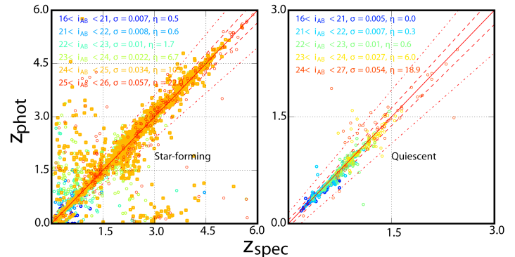
Figure 11.— Comparison between photometric and spectroscopic redshifts as a function of $i_{\rm AB}$ magnitude and type: star-forming galaxies(Left) and quiescent galaxies (Right), keeping only non-flagged galaxies. The dashed and dashed-dot lines show $z_{\rm p}=z_{\rm s}\pm 0.05(1+z_{\rm s})$ and $z_{\rm p}=z_{\rm s}\pm 0.15(1+z_{\rm s})$, respectively.

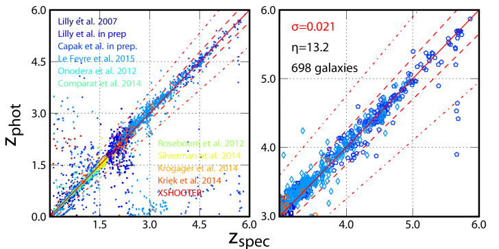
Figure 12.— Left: comparison between photometric and spectroscopic redshifts for the different samples summarized in Table 5. Right: a magnified view of the high-redshift region. The number of galaxies, accuracy $\sigma$ and numbers of catastrophic failures $\eta$ and $\eta_{\rm lim}$ are computed from the zCOSMOS-faint, VUDS, DEIMOS, FMOS, and MOSDEF spectroscopic surveys taken together, keeping only non-flagged galaxies with a spectroscopic redshift greater than 2.9. The dashed and dashed-dot lines show $z_{\rm p}=z_{\rm s}\pm 0.05(1+z_{\rm s})$ and $z_{\rm p}=z_{\rm s}\pm 0.15(1+z_{\rm s})$, respectively. Note that the given value for the precision and the percentage of catastrophic failures strongly depend on the spectroscopic sample. These values are detailed in Table 5.

Table 4Performance of the catalog as a function of magnitude and galaxy types for galaxies detected both in COSMOS2015 and Ilbert et al. (2013) compared to spectroscopic samples. In almost all cases, photometric redshift precision ($\sigma_{13}$ and $\sigma_{15}$) increases and the number of catastrophic failures ( $\eta_{\rm 13}$ and $\eta_{\rm 15}$) fall compared to Ilbert et al. (2013) for a selection common to both catalogs.

	Star-forming galaxies				Quiescent galaxies
$i^{+}$	$\sigma_{15}$	$\eta_{\rm 15}$	$\sigma_{13}$	$\eta_{\rm 13}$	$\sigma_{15}$	$\eta_{\rm 15}$	$\sigma_{13}$	$\eta_{\rm 13}$
		(%)		(%)		(%)		(%)
$[$16,21$]$	0.007	0.5	0.008	0.5	0.005	0.0	0.005	0.0
$[$21,22$]$	0.008	0.6	0.008	0.6	0.007	0.3	0.006	0.4
$[$22,23$]$	0.01	1.7	0.01	1.9	0.01	0.6	0.011	0.6
$[$23,24$]$	0.022	6.7	0.022	7.2	0.027	6.0	0.030	4.4
$[$24,25$]$	0.034	10.2	0.037	15.0	0.054	18.9	0.062	16.7
$[$25,26$]$	0.057	22.0	0.058	24.2

Table 5Characteristics of the spectroscopic redshift samples and photometric redshift accuracy for the objects in a clean (non-flagged) regions. Only the most secure spectroscopic redshifts are considered (those with a flag between 3 and 4). The redshift range, median redshift and apparent magnitude in $i^{+}$-band are provided for each selected sample.

spectroscopic survey /reference	Instrument/	Nb	$z_{\rm med}$	$z_{\rm range}$	$i^{+}_{\rm med}$	$\sigma_{\Delta z/(1+z)}$	$\eta$
	Telescope	spec-z					(%)
zCOSMOS-bright (Lilly et al., 2007)	VIMOS/VLT	8608	0.48	[0.02,1.19]	21.6	0.007	0.51
Comparat et al. (2015)	FORS2/VLT	788	0.89	[0.07,3.65]	22.6	0.009	2.03
Capak et al. in prep, Kartaltepe et al. (2010)	DEIMOS/Keck II	2022	0.93	[0.02,5.87]	23.2	0.014	7.96
Roseboom et al. (2012)	FMOS/Subaru	26	1.21	[0.82,1.50]	22.5	0.009	7.69
Onodera et al. (2012)	MOIRCS/Subaru	10	1.41	[1.24,2.09]	23.9	0.017	0.00
FMOS-COSMOS (Silverman et al., 2015)	FMOS/Subaru	178	1.56	[1.34,1.73]	23.5	0.022	1.12
WFC3-grism (Krogager et al., 2014)	WFC3/HST	11	2.03	[1.88,2.54]	25.1	0.069	0.00
zCOSMOS-faint (Lilly et al. in prep)	VIMOS/VLT	767	2.11	[1.50,2.50]	23.8	0.032	7.95
MOSDEF (Kriek et al., 2015)	MOSFIRE/Keck I	80	2.15	[0.80,3.71]	24.2	0.042	10.0
Stockmann et al. in prep, Zabl (2015)	XSHOOTER/VLT	14	2.19	[1.98,2.48]	22.2	0.061	7.14
VUDS (Le Fevre et al., 2015)	VIMOS/VLT	998	2.70	[0.10,4.93]	24.6	0.028	13.13

Note that the X-ray detected sources from XMM-COSMOS (Hasinger et al., 2007; Cappelluti et al., 2007; Brusa et al., 2010) and Chandra COSMOS (Elvis et al., 2009; Civano et al., 2012) are flagged and not used here. For those sources, the photometric redshift are computed with a specific tuning and are presented in Salvato et al. (2011).

4.4. Photometric redshift accuracy based on the Probability Distribution Function

We also assess the photometric redshift accuracy using the 1$\sigma$ uncertainty derived from the photometric redshift Probability Distribution Function (PDFz). The advantage of this method is that we can investigate the photometric redshift accuracy in any redshift-magnitude range. However, it requires an accurate estimate of the PDFz.

In Figure 13, we show the cumulative distribution of the ratio $|z_{p}-z_{s}|/{{1\sigma}}$.The $1\sigma$ error given by LePhare is defined as the value enclosing 68% of the probability distribution function of the photometric redshift. Assuming that $z_{\rm s}$ is the true redshift, 68% of the times it should fall within the $1\sigma$ error. This comparison shows that the $1\sigma$-uncertainties enclose less than the 68% of the expected value. This is confirmed when we split the spectroscopic sample per magnitude and redshift bin. It appears that our errors on photometric redshift are underestimated by a factor which depends on the magnitude. We consequently chose to correct these errors by applying the following magnitude-dependent correction: errors are multiplied by a factor of 1.2 for bright objects ($i^{+}<20$) and by a factor of $(0.1\times i^{+}-0.8)$ for faint objects ($i^{+}>20$). This issue was already present in previous COSMOS photometric redshift catalogs derived with LePhare, and we have not been able to determine why photometric redshift errors are underestimated; one reason could be the lack of representativity of our set of templates, while another reason could be that we do not include the intrinsic template uncertainties. Another reason might be that the flux uncertainties in the photometric catalog are still be underestimated. With this magnitude-dependent correction, there is no consequence on the computation of the physical parameters. However, the PDFz remains systematically too peaky around the median values.

Figure 14 shows the 1$\sigma$ negative and positive uncertainties as a function of redshift for different bins of apparent magnitude. The magnitude-dependent correction described above has been applied to this plot. Several clear conclusions emerge: first, the photometric precision is lower for galaxies with fainter apparent magnitudes at all redshifts; second, the photometric redshifts have significantly lower uncertainties at $z\lesssim 1.4$. This is easy to understand because here the Balmer break is redshifted within the wavelength range covered by medium bands. At $1.4\lesssim z\lesssim 2.5$, the redshift uncertainty increases by a factor of two. Such a trend is to be expected: the accuracy of the photometric redshift is mainly driven by an accurate knowledge of the Balmer break position. Specifically, at $z>1.5$, the Balmer break moves outside the medium bands into the NIR range. Moreover, the absolute photometric precision is lower for a given signal-to-noise object in the near-infrared bands than in the optical. Additionally, the position of the Balmer break is less precisely determined using broad-band rather than medium-band photometry. This is reflected in the redshift uncertainty which rises at $z>1.5$. For the same reason, we observe a difference in the redshift uncertainties which are lower in ${\cal A}^{\rm UD}$ compared to ${\cal A}^{\rm Deep}$ regions, which is not the case at $z<1.4$: the photometric accuracy is higher in ${\cal A}^{\rm UD}$ regions. At $z\sim 2.5$, the Lyman-break enters into the optical bands and consequently the photometric redshift precision increases. In general, at bright magnitudes and lower redshifts, the dominant sources of error are probably related to photometric calibrations and spectral energy distribution (SED) fitting.

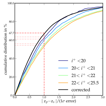
Figure 13.— Cumulative distribution of $|z_{\rm phot}-z_{\rm spec}|/1\sigma$. Of the spectroscopic redshifts, 58% have their photometric redshift within the 1$\sigma$ error; this implies that photometric errors are slightly underestimated. This plot is made with the high-confidence spectroscopic redshift catalog.

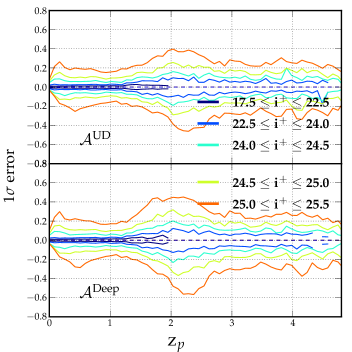
Figure 14.— Bottom and top panels: 1$\sigma$ photometric redshift error as a function of redshift for different magnitude bins on ${\cal A}^{\rm Deep}$ and on ${\cal A}^{\rm UD}$.

4.5. Star/galaxy classification

We use LePhare with both galaxy and stellar templates. We compare the best-fitting $\chi^{2}$ for the galaxy templates $\chi^{2}_{\rm gal}$ and the ones derived for the stellar templates $\chi^{2}_{\rm stars}$ to determine star-galaxy classification. We flag as stars all objects for which $\chi^{2}_{\rm gal}-\chi^{2}_{\rm stars}>0$ but only if the object is detected in NIR or IRAC ($m_{3.6\mu m}\leq 25.5$ or $K_{\rm s}<24.7$) and is not too far from the $BzK$ stellar sequence ($z^{++}-K_{\rm s}<(B-z^{++})*0.3-0.2$).

Figure 15 shows a $BzK$ color-color diagram for all of the sources including stars and galaxies. Symbols are colored according to their photometric redshifts. As expected, $B$-drop-outs occur predominately at $z>4$, and galaxies with bluer $z^{++}-K$ color are at lower redshifts. Stars selected using the above classification are shown in black. In the ${\cal A}^{\rm UVISTA}$ region, 24,074 objects are classified as stars. A cross-match with the ACS stellar catalog Leauthaud et al. (2007) shows that 77% of the stars with $i^{+}<24$ from ACS are classified as stars with this method. However, 15% are misclassified as galaxies but are in masked areas. Finally, 0.6% of the extended sources are misclassified as stars.

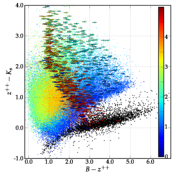
Figure 15.— Color-color diagram $z^{++}-K_{\rm s}$/$B-K_{\rm s}$ for all sources. Sources classified as stars are represented in black. Colors represent redshift. Right-pointing arrows are the upper limits in the $B$ band.

4.6. Absolute magnitudes and stellar masses

An estimate of the $k$-correction term (Oke & Sandage, 1968) relies on the best-fitting template. This component is one of the main sources of systematic error in the absolute magnitude and rest-frame color estimate. To estimate these quantities, we follow the method outlined in Appendix A of Ilbert et al. (2005). In order to minimize the k-correction-induced uncertainties, the rest-frame luminosity at a given wavelength $\lambda$ is derived from the apparent magnitude $m_{obs}$ observed at the nearest filter to $\lambda(1+z)$. Using this procedure, the absolute magnitudes are less dependent on the best-fit SED, but are more dependent on any observational problem affecting $m_{\rm obs}$. Therefore, we constrain the code to consider only the broad bands for $m_{\rm obs}$ and those bands with a systematic offset lower than 0.1 mag derived for the photometric redshift.

We derive the stellar mass using LePhare following exactly the same method as in Ilbert et al. (2015). We derive the galaxy stellar masses using a library of synthetic spectra generated using the Stellar Population Synthesis (SPS) model of Bruzual & Charlot (2003). We assume a Chabrier (2003) Initial Mass Function (IMF). We combine the exponentially declining SFH and delayed SFH ($\tau^{-2}te^{-t/\tau}$). Two metallicities (solar and half-solar) are considered. Emission lines are added following Ilbert et al. (2009). We include two attenuation curves: the starburst curve of Calzetti et al. (2000) and a curve with a slope $\lambda^{−0.9}$ (Appendix A of Arnouts et al., 2013). The $E(B-V)$ values are allowed to take values as high as 0.7. We assign the mass using the median of the marginalized probability distribution function (PDF). Given the uncertainties on the SFR based on template fitting (Ilbert et al., 2015; Lee et al., 2015) we do not include the SFRs estimated from template fitting in our distributed catalogs.

5. Characteristics of the global sample

5.1. Galaxy classification

Quiescent galaxies can be identified using the locations of galaxies in the color-color plane NUV-$r$/$r$-$J$ (Williams et al., 2009). Quiescent objects are those with $M_{NUV}-M_{r}>3(M_{r}-M_{J})+1$ and $M_{NUV}-M_{r}>3.1$. This technique is described in more detail in Ilbert et al. (2013); in particular, this technique avoids mixing the red dusty galaxies and quiescent galaxies. In our catalog, galaxies with a flag of 0 are quiescent galaxies and the others are star-forming galaxies. The redshift-dependent evolution of this distribution is presented in figure 16. The rapid build-up of quiescent galaxies at low redshift inside the box is evident, as is the relative decrease in bright, star-forming galaxies outside the box.

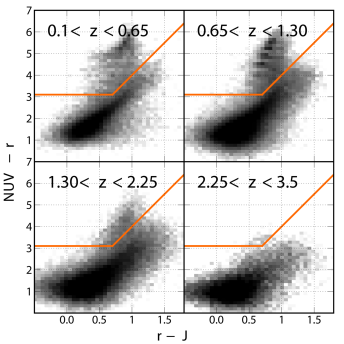
Figure 16.— NUV$-r$/$r-J$ galaxy distributions. Quiescent galaxies lie in the top-left corner. The objects fainter than limiting magnitudes are not used.

5.2. Stellar mass Completeness

We empirically estimate the stellar mass completeness (Pozzetti et al., 2010; Ilbert et al., 2013; Moustakas et al., 2013; Davidzon et al., 2013). We first determine the magnitude limit $K_{\rm s\,lim}$. For each galaxy, we then determine the mass it would need to have to be observed, at that redshift, at the magnitude limit:

$$\log M_{\rm lim}=\log M-0.4(K_{\rm s\,lim}-K_{\rm s}).$$ (7)

Next, in each redshift bin, we independently estimate the stellar mass completeness $M_{\rm lim}$ within which 90% of the galaxies lie. We estimate independently the mass limits on ${\cal A}^{\rm Deep}$ and ${\cal A}^{\rm UD}$. We compute these mass limits using the 3$\sigma$ limiting magnitude, which is 24.0 for ${\cal A}^{\rm Deep}$ and 24.7 for ${\cal A}^{\rm UD}$. These mass limits are given in Table 6 and are shown in Figure 17. In ${\cal A}^{\rm UD}$, the mass limits reach a factor of two lower in mass compared Ilbert et al. (2013). As expected, the mass limit is lower in ${\cal A}^{\rm UD}$ compared to ${\cal A}^{\rm Deep}$, because ${\cal A}^{\rm UD}$ reaches 0.7 magnitudes fainter in the $K_{\rm s}$ band. This estimate is robust to $z\sim 4$ because the observed $K_{\rm s}$ magnitude correlates well with stellar mass in this redshift range. However, these estimates should be treated cautiously at $z>4$. Above this redshift, the rest-frame $K_{\rm s}$ band lies below the Balmer break and the $K_{\rm s}$ flux does not correspond precisely to the stellar mass. It is then better traced by mid-IR bands. We will estimate the mass limit at high redshift for an IRAC-selected sample in a future work (Davidzon et al. in preparation).

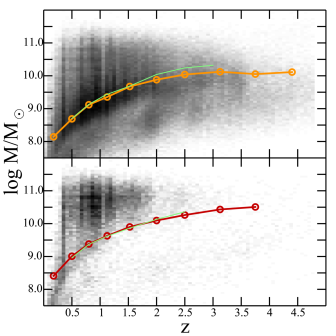
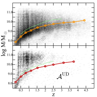
Figure 17.— Stellar mass-redshift histogram (the grayscale corresponds to the the number of galaxies in each cell) on ${\cal A}^{\rm Deep}$ (left) and ${\cal A}^{\rm UD}$ (right) regions for the full catalog (top) and for the quiescent sample (bottom). Orange lines shows the mass limit for the full catalog and red lines for the quiescent ones. These values are reported in Table 6. The solid green line is the mass limit in COSMOS as given in Ilbert et al. (2013).

Table 6Mass limits of COSMOS2015 for the full, quiescent and the star-forming samples in the ${\cal A}^{\rm Deep}$ and ${\cal A}^{\rm UD}$ regions. $N_{\rm gal}^{\rm full}$, $N_{\rm gal}^{\rm quies}$, $N_{\rm gal}^{\rm SF}$ are the percentage of galaxies in each redshift bins for the full, quiescent, and star forming populations. $M_{\rm lim}^{\rm full}$, $M_{\rm lim}^{\rm quies}$, $M_{\rm lim}^{\rm SF}$ are the logarithm of the limiting mass in units of solar masses.

	${\cal A}^{\rm Deep}$						${\cal A}^{\rm UD}$
bin	$N_{\rm gal}^{\rm full}$	$M_{\rm lim}^{\rm full}$	$N_{\rm gal}^{\rm quies}$	$M_{\rm lim}^{\rm quies}$	$N_{\rm gal}^{\rm SF}$	$M_{\rm lim}^{\rm SF}$	$N_{\rm gal}^{\rm full}$	$M_{\rm lim}^{\rm full}$	$N_{\rm gal}^{\rm quies}$	$M_{\rm lim}^{\rm quies}$	$N_{\rm gal}^{\rm SF}$	$M_{\rm lim}^{\rm SF}$
0.00$<z<$0.35	8.6	8.1	11.3	8.4	8.3	8.1	9.0	7.9	13.8	8.1	8.7	7.8
0.35$<z<$0.65	14.1	8.7	18.4	9.0	13.7	8.6	13.5	8.4	19.2	8.7	13.0	8.4
0.65$<z<$0.95	17.4	9.1	27.4	9.4	16.7	9.0	17.5	8.9	27.4	9.1	16.7	8.7
0.95$<z<$1.30	16.4	9.3	20.5	9.6	16.1	9.2	16.3	9.1	18.9	9.3	16.1	9.0
1.30$<z<$1.75	14.2	9.7	12.5	9.9	14.4	9.6	14.9	9.4	11.8	9.6	15.2	9.3
1.75$<z<$2.25	12.0	9.9	4.9	10.1	12.5	9.8	11.0	9.6	4.0	9.8	11.5	9.6
2.25$<z<$2.75	6.8	10.0	2.4	10.3	7.1	10.0	6.5	9.8	2.2	10.0	6.8	9.8
2.75$<z<$3.50	6.4	10.1	1.4	10.4	6.8	10.1	7.1	9.9	1.5	10.2	7.5	9.9
3.50$<z<$4.00	1.9	10.1	0.5	10.5	2.0	10.5	2.0	10.0	0.4	10.3	2.1	10.0
4.00$<z<$4.80	1.4	10.1	-	-	1.5	10.8	1.5	10.2	-	-	1.6	10.1

5.3. Galaxy clustering measurements

We estimate the projected galaxy clustering in our sample by computing the angular two-point auto-correlation function $w(\theta)$. The angular correlation function $w(\theta)$ measures the excess probability of finding two objects separated by an angle $\theta$ compared to a random distribution in a series of angular bins. This measurement is an excellent test of the uniformity of our photometric catalog as $w$ is very sensitive to large-scale photometric systematic errors. Adding cuts in stellar mass and photometric redshift allows for an independent check of our photometric redshift procedures. We $w$ to compute this using ATHENA, which uses the usual Landy & Szalay (1993) estimator:

$$w(\theta)=\frac{1}{RR}\times\left(\frac{N_{r}(N_{r}-1)}{N_{d}(N_{d}-1)}DD-2\frac{N_{r}}{N_{d}}DR+RR\right)$$ (8)

Where $N_{r}$ and $N_{d}$ are the number of points in the random and the galaxy sample, and $RR$, $RD$ and $DD$ are the number of pairs in the random catalog, between the random and galaxy catalog, and in the galaxy catalog. Our random catalog contains 500,000 objects. Our measurements are corrected for the “integral constraint” (Growth & Peebles, 1977), a systematic effect arising from using a clustered sample to estimate the mean background density in a finite area.

Figure 18 shows $w$ in $0.5<z<1$ in six mass bins compared to the best-fitting occupation distribution (HOD) model derived by Coupon et al. (2015) in the MIRACLES/CFHTLS field. Our measurements are in excellent agreement with the predictions of Coupon et al.’s best-fitting HOD model, computed from a larger 25deg ² field. This suggests that, at these redshift ranges and masses, cosmic variance is not an important issue in the COSMOS field. Only at high stellar masses and small scales is there a systematic offset from the models, which may indicate the limitations of the halo model in this mass regime.

Finally, we note that, in contrast to this result, some works have noted that there is a clear excess in the number of galaxies in COSMOS compared to other fields (see, e.g, Figure 33 in Molino et al., 2014) due to the presence of large structures at $z\sim 1$ and below, which could influence our correlation function measurements (McCracken et al., 2007). The measurements presented above cover quite a large redshift range and consequently probe a lare volume, and are therefore less susceptible to the effects of cosmic variance. In smaller redshift slices and at higher redshifts, the effect of cosmic variance becomes more pronounced, especially when these redshift ranges overlap with several of the large structures known to exist in the COSMOS field, for example, at $1<z<1.3$ (see also the discussion in McCracken et al., 2015).

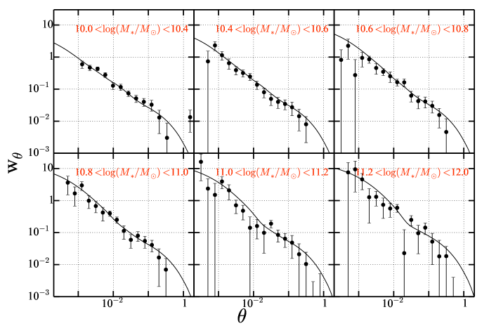
Figure 18.— Angular correlation function $w$ as a function of angular scale $\theta$ in degrees at $0.5<z<1$ for several bins in stellar mass. The solid line shows the analytic predictions of Coupon et al. (2015).

6. Conclusion

Using the unique combination of deep multi-wavelength data and spectroscopic redshifts on the COSMOS field, we have computed a new catalog containing precise photometric redshifts and 30-band photometry. COSMOS2015 contains more than half a million secure objects over two square degrees. Including new $YJHK_{\rm s}$ images from the UltraVISTA-DR2 survey, $Y$-band images from Hyper Suprime-Cam and IR data from the SPLASH Spitzer legacy program, this NIR-selected catalog is highly optimized for the study of galaxy evolution and environment in the early Universe. To maximize catalog completeness to the highest redshifts, objects have been detected and selected using an ultra-deep $\chi^{2}$ sum of the $YJHK_{\rm s}$ and $z^{++}$ images.

The main improvements of the catalog compared with previous versions are as follows.

• A great number of sources thanks to the combination of deeper data (UltraVISTA-DR2) and an improved extraction image. This image now contains the bluer $z^{++}$ band in addition to the redder NIR bands. There are now $\sim 6\times 10^{5}$ objects in the 1.5 deg² UltraVISTA-DR2 area and $\sim 1.5\times 10^{5}$ in the “ultra-deep stripes” sub-region at the limiting magnitude in $K_{\rm s}$. This represents more than twice as many objects per square degree compared to Ilbert et al. (2013).

• More precise photometric redshifts. Based on comparisons with the unique spectroscopic redshift sample in the COSMOS field, we measure $\sigma_{\Delta z/(1+z_{s})}$ = 0.021 for $3<z<6$ with 13.2% of outliers. At lower redshifts, the precision is better than 0.01, only a few percent of catastrophic failures. The precision at low redshifts is consistent with Ilbert et al. (2013), while it improves significantly at high redshift.

• The characteristic mass limits are much lower. The deepest regions reach a completeness limit of 10${}^{10}M_{\odot}$ to $z=4$, which is more than 0.3 dex better compared to Ilbert et al. (2013) for the full sample.

Detailed comparisons of the color distributions, number counts and clustering show good agreement with the literature in the mass ranges where these previous studies overlap with ours. In particular, our mass-selected clustering measurements at $0.5<z<1$ are in excellent agreement with Coupon et al.’s halo model calibrated using $25~{}\deg^{2}$ of the CFHTLS.

The COSMOS2015 catalog represents an invaluable resource which can be used to investigate the evolution of galaxies and structures back to the earliest stages of the Universe. Sampling the galaxy population out to $z\sim 4$ at degree scales it will allow us to study the connection between galaxies, their host dark matter haloes, and their large-scale environment, back to the earliest epochs of cosmic time.

7. Appendix

7.1. Catalog description

The details of the regions flagged in the catalog are presented in Table 7. We perform COSMOS2015 quality checks only in the inner part of the field covered by UltraVISTA-DR2. On the part of the field not covered by UltraVISTA, the source extraction is performed only on the $z^{++}$-band data and using the same parameters. This part of the field has a higher fraction of spurious sources and must be exploited carefully, particularly when selecting a mass-selected sample. The area referred as ${\cal A}^{\rm Deep}$ above is the region covered by ${\cal A}^{\rm UVISTA}$ not containing ${\cal A}^{\rm UD}$.

Table 7Names, effective area, number of objects and coordinates of the regions flagged in the catalog and plotted in Figure 1. The region files are distributed with the catalog.

Name	Area	Nbr of	Coordinates or description
	deg2	objects
${\cal A}^{\rm COSMOS}$	2	773118	poly(148.70,0.79,151.53,3.620)
${\cal A}^{\rm!OPT}$ & ${\cal A}^{\rm COSMOS}$	1.77	694478	not flagged regions in the optical bands inside the COSMOS 2deg2 field
${\cal A}^{\rm UD}$	0.62	247203	poly(150.58,2.71,150.42,2.72,150.41,2.43,150.42,
			1.871,150.50,1.88,150.49,1.99,150.59,1.99)
			poly(150.21,2.71,150.05,2.71,150.06,1.71,150.22,1.70,150.2,2.66)
			poly(149.84,2.71,149.68,2.71,149.68,1.71,149.85,1.70,149.84,2.66)
			poly(149.48,2.71,149.33,2.72,149.32,1.71,149.49,1.71,149.48,2.66)
${\cal A}^{\rm UVISTA}$	1.70	646939	poly(150.77,2.81,149.31,2.81,149.32,1.61,150.41,1.61,150.41,1.66,
			150.51,1.66,150.51,1.88,150.54,1.91,150.58,
			1.88,150.59,1.65,150.68,1.66,150.70,1.88,150.79,1.88)
${\cal A}^{\rm UD}$ & ${\cal A}^{\rm COSMOS}$	0.53	213716	Ultra-Deep area inside the COSMOS 2deg2 field
${\cal A}^{\rm UD}$ & ${\cal A}^{\rm!OPT}$ & ${\cal A}^{\rm COSMOS}$	0.46	190650	Ultra-Deep area inside the COSMOS 2deg2 field,
			after removing flagged regions in the optical bands
${\cal A}^{\rm UVISTA}$ & ${\cal A}^{\rm COSMOS}$	1.58	604265	UVISTA area inside the COSMOS 2deg2 field
${\cal A}^{\rm UVISTA}$ & ${\cal A}^{\rm!OPT}$ & ${\cal A}^{\rm COSMOS}$	1.38	536077	UVISTA area inside the COSMOS 2deg2 field,
			after removing flagged regions in the optical bands

The parameters for the extraction of the photometry in dual mode with SExtractor are presented in Table 9.

Each column in the catalog is fully described by a README file distributed with the catalog. We summarize the main content of our data products in Table 8.

7.2. From aperture magnitudes to total magnitudes

Finally, we emphasize that to compute thr total magnitudes, one should use 3$\arcsec$ diameter apertures, corrected for the photometric offsets ($o_{i}$, cf. Equation 4) and systematic offsets ($s_{f}$, cf. Table 3) according to the formula

$${\rm MAG\_TOTAL}_{i,f}={\rm MAG\_APER3}_{i,f}+o_{i}-s_{f}$$ (9)

where $i$ is the object identifier and $f$ the filter identifier. A similar procedure should be followed for the flux measurements. Magnitudes should also be corrected for foreground galactic extinction using reddenning values $EBV$ given in the catalog and the extinction factors ($F_{\rm f}$) mentioned in Table 3 according to

$${\rm MAG\_TOTAL}_{i,f}={\rm MAG\_TOTAL}_{i,f}-EBV_{\rm i}*F_{\rm f}$$ (10)

Table 8Summary of the main photometric and $z$-phot catalog columns. Matches with publicly available radio catalogs on COSMOS field are also provided. Please refer to the README file distributed with the catalog for more information.

General Parameters
ID	-	identifiant
ALPHA_2000, BETA_2000	deg	Ra and Dec
X_IMAGE, Y_IMAGE	pix	pixel position
ERRX2_IMAGE, ERRY2_IMAGE, ERRXY_IMAGE	pix	variances and covariance on positional measurements
FLAGS_#$\left[{\rm Name\,of\,flag}\right]$	-	flags as described in Table 7
EBV		Galactic extinction (Schlegel et al., 1998)
optical and NIR photometry
#$\left[{\rm band}\right]$ _FLUX_APER2, #$\left[{\rm band}\right]$_FLUXERR_APER2	$\mu$Jy	flux and flux error measured in a 2$\mathrm{\SIUnitSymbolArcsecond}$ aperture
#$\left[{\rm band}\right]$_FLUX_APER3, #$\left[{\rm band}\right]$_FLUXERR_APER3	$\mu$Jy	flux and flux error measured in a 3$\mathrm{\SIUnitSymbolArcsecond}$ aperture
#$\left[{\rm band}\right]$_MAG_APER2, #$\left[{\rm band}\right]$_MAGERR_APER2	mag	magnitude and magnitude error measured in a 2$\mathrm{\SIUnitSymbolArcsecond}$ aperture
#$\left[{\rm band}\right]$_MAG_APER3, #$\left[{\rm band}\right]$_MAGERR_APER3	mag	magnitude and magnitude error measured in a 3$\mathrm{\SIUnitSymbolArcsecond}$ aperture
#$\left[{\rm band}\right]$_MAG_AUTO, #$\left[{\rm band}\right]$_MAGERR_AUTO	mag	automatic aperture magnitude and magnitude error
#$\left[{\rm band}\right]$_MAG_ISO, #$\left[{\rm band}\right]$_MAGERR_ISO	mag	isophotal magnitude and magnitude error
#$\left[{\rm band}\right]$_FLAGS		flags from SExtractor
Match with the 24$\mu$m MIPS catalog (Le Floc’h et al., 2009)
24_FLUX, 24_FLUXERR	$\mu$Jy	total flux and flux error
Match with the PACS/PEP catalog (Lutz et al., 2011)
100_FLUX, 100_FLUXERR	mJy	total 100$\mu$m flux and flux error
160_FLUX, 160_FLUXERR	mJy	total 160$\mu$m flux and flux error
Match with the SPIRE/HerMES catalog (Oliver et al., 2012)
250_FLUX, 250_FLUXERR	mJy	total 250$\mu$m flux and flux error
350_FLUX, 350_FLUXERR	mJy	total 350$\mu$m flux and flux error
500_FLUX, 500_FLUXERR	mJy	total 500$\mu$m flux and flux error
GALEX photometry (Capak et al., 2007)
FLUX_GALEX_NUV, FLUXERR_GALEX_NUV	mJy	total flux and flux error
FLUX_GALEX_FUV, FLUXERR_GALEX_FUV	mJy	total flux and flux error
Match with the Chandra COSMOS-Legacy survey (Elvis et al., 2009; Civano et al., 2012, 2016; Marchesi et al., 2016)
IDChandra	-	corresponding identifiant in the Chandra catalog
Match with ACS (Leauthaud et al., 2007)
814W_FLUX, 814W_FLUXERR	$\mu$Jy	flux and flux error for automatic aperture
Match with previous multi-bands catalog
ID2006	-	identifiant in the $1^{\rm st}$ version of the catalog from Capak et al. (2007)
ID2008	-	identifiant in the $2^{\rm nd}$ version of the catalog from Capak et al. (2007)
ID2013	-	corresponding identifiant in the catalog from Ilbert et al. (2013)
Parameters computed with LePhare
total_off	mag	weighted offset from MAG_APER3 to total mag
type	-	0 if galaxy, 1 if star, 2 if Xray source, -9 if failure in the fit
zPDF	-	median of the likelihood distribution
zPDF_l68, zPDF_u68	-	lower and upper limits (68% confidence level)
zMinChi2	-	photo-z defines as the minimum of the $\chi^{2}$ distribution.
chi2best	-	reduced chi2 (-99 if less than 3 filters) for zMinChi2
zp_2	-	2nd photo-z solution if a second peak is detected with P$>$5% in the PDF
chi2_2	-	reduced chi2 for the second photo-z solution
NbFilt	-	number of filters used in the fit
zq, modq, chiq	-	z for the AGN library, best fit template and associated reduced $\chi^{2}$
mods, chis	-	model for the star library and associated reduced $\chi^{2}$
model, age, extinction	-	best fit BC03 model at zPDF
M_#$\left[{\rm band}\right]$	mag	absolute magnitudes in NUV,$u$,$B$,$r$,$i^{+}$,$z^{++}$,$Y$,$J$,$H$,$K_{\rm s}$
M_NUV-M_R	mag	color corrected from dust-extinction
mass_med	dex	log stellar mass from BC03 best-fit template (median)
mass_med_min68, mass_med_max68	dex	lower and upper limits (68% confidence level)
mass_best	dex	log stellar mass from BC03 best-fit template (minimum $\chi^{2}$)
L_#$\left[{\rm band}\right]$	dex	luminosities in NUV,$r$,$K_{\rm s}$ filters

Table 9SExtractor parameters used for Dual-mode $\chi^{2}$ detection and photometry.

Name	Value
ANALYS_THRESH	1.5
FILTER_NAME	gauss_4.0_7$\times$7.conv
CATALOG_TYPE	FITS_1.0
DETECT_TYPE	CCD
THRESH_TYPE	ABSOLUTE
DETECT_MINAREA	10
DETECT_MAXAREA	100 000
DETECT_THRESH	1.51
FILTER	Y
DEBLEND_NTHRESH	32
DEBLEND_MINCONT	0.00001
CLEAN	Y
CLEAN_PARAM	1.0
MASK_TYPE	CORRECT
PHOT_APERTURES	13.33, 20.00, 47.33
PHOT_AUTOPARAMS	2.5, 3.5
PHOT_FLUXFRAC	0.2, 0.5, 0.8
PHOT_AUTOAPERS	13.3, 13.3
SATUR_LEVEL	30000.
MAG_ZEROPOINT	depends on the band
GAIN	depends on the band
PIXEL_SCALE	4.16666$\times 10^{-5}$
BACK_SIZE	128
BACK_FILTERSIZE	3
BACKPHOTO_TYPE	LOCAL
BACKPHOTO_THICK	30
WEIGHT_GAIN	N
RESCALE_WEIGHTS	N
WEIGHT_TYPE	depends on the band
GAIN_KEY	DUMMY

7.3. Effect of the seeing on the aperture magnitude

As discussed in section 2.2, there is a variation of the PSF within the field which is not taken into account in our homogenization. For this reason, it is important to estimate the magnitude differences arising from this variation. To achieve this, we present here a toy model to estimate the effect of the seeing variation on the aperture magnitude for point-like objects. We denote $D_{\rm stars}$($\theta$,$\beta$,$r$) as the difference of the aperture magnitudes for a PSF represented by a Moffat profile ${\cal M}\left[\theta,\beta\right]$ and with a PSF ${\cal M}\left[0.8\arcsec,2.5\right]$. $D_{\rm stars}$ is a function of $\theta$ and $\beta$, the two parameters which define the Moffat profile, and $r$ which is the aperture diameter. We present in Figure 19 $D_{\rm stars}$($\theta$,$\beta$,3$\arcsec$) in the two-dimensional (2D) parameter space $\left[\theta,\beta\right]$. We overplotted on this 2D distribution the contours which enclose 68% and 95% of the [$\theta$,$\beta$] distribution for the two bands $u$ and $IA464$. For the purpose of this figure, each star seeing is individually computed from a fit with a Moffat profile on the PSF-homogenized star profiles (reconstructed from the flux extracted at 14 fixed apertures, logarithmically spaced between 0.25$\arcsec$ and 2.5$\arcsec$). Note that since the Moffat Profile is fitted on individual stars from 14 discrete apertures and not on all of the point sources at the same time, the precision of the fit is limited. However, this immediately provides a qualitative insight as to the bias generated by internal PSF variation when extracting the star photometry within a 3$\arcsec$ aperture. For the worst band $IA464$, this bias is expected to remain below 0.1 mag. We also estimate that the median of the magnitude difference is below 0.05 mag, which is in agreement with Figure 4.

We then estimate this bias in the photometry for extended objects. We chose two different galaxy luminosity profiles, namely, a de Vaucouleurs profile (1948, 1959) to model a typical elliptical galaxy profile,

$$F_{\rm elliptical}(R_{e},r)\propto\exp\left[-7.67\left(\frac{r}{R_{e}}\right)^{\frac{1}{4}}\right]$$ (11)

and an exponential profile to model a spiral galaxy profile,

$$F_{\rm spiral}(R_{e},r)\propto\exp\left[-\frac{r}{R_{e}}\right]$$ (12)

Here, $R_{e}$ is the effective radius such that half of the total flux is within $R_{e}$. We then convolved the luminosity profiles with the Moffat profile, and integrate them in a circular aperture of 3$\arcsec$. For this exercise, we keep $\beta$ constant and equal to 2.5 and we allow $\theta$ to vary. In Figure 20, we present the difference $D_{\rm spiral}$($\theta$,2.5,1.5$\arcsec$) and $D_{\rm elliptical}$($\theta$,2.5,1.5$\arcsec$) for two effective radii ($R_{e}=$ 0.5 and 0.8 $\arcsec$). We note that for FWHM differences below 0.1$\arcsec$ the induced magnitude discrepancies are always lower than 0.05, regardless of the galaxy profile.

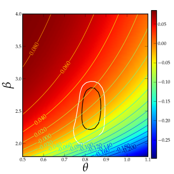
Figure 19.— Magnitude difference (measured in $3\mathrm{\SIUnitSymbolArcsecond}$ diameter apertures) between a point-like object convolved with the target PSF ${\cal M}\left[0.8\mathrm{\SIUnitSymbolArcsecond},2.5\right]$ and with ${\cal M}\left[\theta,\beta\right]$ in the 2D parameter space $\left[\theta\mathrm{\SIUnitSymbolArcsecond},\beta\right]$. The black and white contours represent the regions which enclose 68% and 95% of the $\beta$-$\theta$ stellar distribution for two representative bands: $u$ (Left), which is relatively homogenous across the field, and $IA464$ which is not.

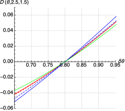
Figure 20.— Magnitude difference for a point-like object (green), an elliptical galaxy (red), and a spiral galaxy (blue) convolved with a PSF ${\cal M}\left[\theta,2.5\right]$ as a function of the seeing $\theta$ and for two different effective radii, 0.5 $\arcsec$ (solid line) and 0.8 $\arcsec$ (dashed line), when the extraction is performed in 3 $\arcsec$ diameter apertures.

References

- Aihara et al. (2011) Aihara, H., Allende Prieto, C., An, D., et al. 2011, ApJS, 193, 29
- Allen (1976) Allen, C. W. 1976, Astrophysical Quantities, 4th edn. (Addison-Wesley Professional)
- Arnouts et al. (2002) Arnouts, S., Moscardini, L., Vanzella, E., et al. 2002, MNRAS, 329, 355
- Arnouts et al. (2007) Arnouts, S., Walcher, C. J., Le Fèvre, O., et al. 2007, A&A, 476, 137
- Arnouts et al. (2013) Arnouts, S., Le Floc’h, E., Chevallard, J., et al. 2013, A&A, 558, A67
- Bertin (2013) Bertin, E. 2013, PSFEx: Point Spread Function Extractor, Astrophysics Source Code Library, ascl:1301.001
- Bertin & Arnouts (1996) Bertin, E., & Arnouts, S. 1996, ApJS, 117, 393
- Bertin et al. (2002) Bertin, E., Mellier, Y., Radovich, M., et al. 2002, Astronomical Data Analysis Software and Systems XI, 281, 228
- Béthermin et al. (2014) Béthermin, M., Kilbinger, M., Daddi, E., et al. 2014, A&A, 567, A103
- Bielby et al. (2012) Bielby, R., Hudelot, P., McCracken, H. J., et al. 2012, A&A, 545, 23
- Bieri et al. (2015) Bieri, R., Dubois, Y., Silk, J., & Mamon, G. A. 2015, ApJ, 812, L36
- Bolzonella et al. (2000) Bolzonella, M., Miralles, J.-M., & Pelló, R. 2000, A&A, 363, 476
- Brusa et al. (2010) Brusa, M., Civano, F., Comastri, A., et al. 2010, ApJ, 716, 348
- Bruzual & Charlot (2003) Bruzual, G., & Charlot, S. 2003, MNRAS, 344, 1000
- Calzetti et al. (2000) Calzetti, D., Armus, L., Bohlin, R. C., et al. 2000, ApJ, 533, 682
- Capak et al. (2007) Capak, P., Aussel, H., Ajiki, M., et al. 2007, ApJS, 172, 99
- Cappelluti et al. (2007) Cappelluti, N., Hasinger, G., Brusa, M., et al. 2007, ApJS, 172, 341
- Chabrier (2003) Chabrier, G. 2003, PASP, 115, 763
- Civano et al. (2012) Civano, F., Elvis, M., Brusa, M., et al. 2012, ApJS, 201, 30
- Civano et al. (2016) Civano, F., Marchesi, S., Comastri, A., et al. 2016, ArXiv e-prints, arXiv:1601.00941
- Codis et al. (2012) Codis, S., Pichon, C., Devriendt, J., et al. 2012, MNRAS, 427, 3320
- Codis et al. (2015) Codis, S., Pichon, C., & Pogosyan, D. 2015, MNRAS, 452, 3369
- Comparat et al. (2015) Comparat, J., Richard, J., Kneib, J.-P., et al. 2015, A&A, 575, A40
- Cooray & Sheth (2002) Cooray, A., & Sheth, R. 2002, Phys. Rep., 372, 1
- Coupon et al. (2015) Coupon, J., Arnouts, S., van Waerbeke, L., et al. 2015, MNRAS, 449, 1352
- Cowie et al. (1996) Cowie, L. L., Songaila, A., Hu, E. M., & Cohen, J. G. 1996, Astronomical Journal v.112, 112, 839
- Croton et al. (2006) Croton, D. J., Springel, V., White, S. D. M., et al. 2006, MNRAS, 367, 864
- Daddi et al. (2007) Daddi, E., Dickinson, M., Morrison, G., et al. 2007, ApJ, 670, 156
- Darvish et al. (2014) Darvish, B., Sobral, D., Mobasher, B., et al. 2014, ApJ, 796, 51
- Davidzon et al. (2013) Davidzon, I., Bolzonella, M., Coupon, J., et al. 2013, A&A, 558, A23
- Dekel et al. (2009) Dekel, A., Birnboim, Y., Engel, G., et al. 2009, Nature, 457, 451
- Dressler (1980) Dressler, A. 1980, ApJ, 236, 351
- Dubois et al. (2014) Dubois, Y., Pichon, C., Welker, C., et al. 2014, MNRAS, 444, 1453
- Elbaz et al. (2007) Elbaz, D., Daddi, E., Le Borgne, D., et al. 2007, A&A, 468, 33
- Elvis et al. (2009) Elvis, M., Civano, F., Vignali, C., et al. 2009, ApJS, 184, 158
- Fioc & Rocca-Volmerange (1997) Fioc, M., & Rocca-Volmerange, B. 1997, A&A, 326, 950
- Fioc & Rocca-Volmerange (1999) —. 1999, ArXiv Astrophysics e-prints, astro-ph/9912179
- Fitzpatrick & Massa (1986) Fitzpatrick, E. L., & Massa, D. 1986, ApJ, 307, 286
- Fontana et al. (2014) Fontana, A., Dunlop, J. S., Paris, D., et al. 2014, A&A, 570, A11
- Gaibler et al. (2012) Gaibler, V., Khochfar, S., Krause, M., & Silk, J. 2012, MNRAS, 425, 438
- Griffin et al. (2010) Griffin, M. J., Abergel, A., Abreu, A., et al. 2010, A&A, 518, L3
- Growth & Peebles (1977) Growth, E. J., & Peebles, P. J. E. 1977, ApJ, 217, 385
- Hasinger et al. (2007) Hasinger, G., Cappelluti, N., Brunner, H., et al. 2007, ApJS, 172, 29
- Heinis et al. (2007) Heinis, S., Milliard, B., Arnouts, S., et al. 2007, ApJS, 173, 503
- Hildebrandt et al. (2012) Hildebrandt, H., Erben, T., Kuijken, K., et al. 2012, MNRAS, 421, 2355
- Hoaglin et al. (1983) Hoaglin, D. C., Mosteller, F., & Tukey, J. W. 1983, Understanding robust and exploratory data anlysis
- Hopkins et al. (2006) Hopkins, P. F., Hernquist, L., Cox, T. J., et al. 2006, ApJS, 163, 1
- Hsieh et al. (2012) Hsieh, B.-C., Wang, W.-H., Hsieh, C.-C., et al. 2012, ApJS, 203, 23
- Ilbert et al. (2005) Ilbert, O., Tresse, L., Zucca, E., et al. 2005, A&A, 439, 863
- Ilbert et al. (2006) Ilbert, O., Arnouts, S., McCracken, H. J., et al. 2006, A&A, 457, 841
- Ilbert et al. (2009) Ilbert, O., Capak, P., Salvato, M., et al. 2009, ApJ, 690, 1236
- Ilbert et al. (2013) Ilbert, O., McCracken, H. J., Le Fèvre, O., et al. 2013, A&A, 556, A55
- Ilbert et al. (2015) Ilbert, O., Arnouts, S., Le Floc’h, E., et al. 2015, A&A, 579, A2
- Kartaltepe et al. (2010) Kartaltepe, J. S., Sanders, D. B., Le Floc’h, E., et al. 2010, ApJ, 721, 98
- Katz et al. (2003) Katz, N., Keres, D., Dave, R., & Weinberg, D. H. 2003, in Astrophysics and Space Science Library, Vol. 281, The IGM/Galaxy Connection. The Distribution of Baryons at z=0, ed. J. L. Rosenberg & M. E. Putman, 185
- Kauffmann et al. (2004) Kauffmann, G., White, S. D. M., Heckman, T. M., et al. 2004, MNRAS, 353, 713
- Kereš et al. (2005) Kereš, D., Katz, N., Weinberg, D. H., & Davé, R. 2005, MNRAS, 363, 2
- Khandai et al. (2015) Khandai, N., Di Matteo, T., Croft, R., et al. 2015, MNRAS, 450, 1349
- Kochiashvili et al. (2015) Kochiashvili, I., Møller, P., Milvang-Jensen, B., et al. 2015, A&A, 580, A42
- Koekemoer et al. (2007) Koekemoer, A. M., Aussel, H., Calzetti, D., et al. 2007, ApJS, 172, 196
- Kriek et al. (2015) Kriek, M., Shapley, A. E., Reddy, N. A., et al. 2015, ApJS, 218, 15
- Krogager et al. (2014) Krogager, J.-K., Zirm, A. W., Toft, S., Man, A., & Brammer, G. 2014, ApJ, 797, 17
- Kron (1980) Kron, R. G. 1980, ApJS, 43, 305
- Laigle et al. (2015) Laigle, C., Pichon, C., Codis, S., et al. 2015, MNRAS, 446, 2744
- Landy & Szalay (1993) Landy, S. D., & Szalay, A. S. 1993, ApJ, 412, 64
- Le Fevre et al. (2015) Le Fevre, O., Tasca, L. A. M., Cassata, P., et al. 2015, A&A, 576, A79
- Le Floc’h et al. (2009) Le Floc’h, E., Aussel, H., Ilbert, O., et al. 2009, ApJ, 703, 222
- Leauthaud et al. (2007) Leauthaud, A., Massey, R., Kneib, J.-P., et al. 2007, ApJS, 172, 219
- Lee et al. (2012) Lee, K.-S., Alberts, S., Atlee, D., et al. 2012, ApJ, 758, L31
- Lee et al. (2015) Lee, N., Sanders, D. B., Casey, C. M., et al. 2015, ApJ, 801, 80
- Libeskind et al. (2013) Libeskind, N. I., Hoffman, Y., Steinmetz, M., et al. 2013, ApJ, 766, L15
- Lilly et al. (2007) Lilly, S. J., Le Fèvre, O., Renzini, A., et al. 2007, ApJS, 172, 70
- Lin et al. (2014) Lin, L., Jian, H.-Y., Foucaud, S., et al. 2014, ApJ, 782, 33
- Lutz et al. (2011) Lutz, D., Poglitsch, A., Altieri, B., et al. 2011, A&A, 532, A90
- Marchesi et al. (2016) Marchesi, S., Civano, F., Elvis, M., et al. 2016, ApJ, 817, 34
- Massey & Refregier (2005) Massey, R., & Refregier, A. 2005, MNRAS, 363, 197
- McCracken et al. (2007) McCracken, H. J., Peacock, J. A., Guzzo, L., et al. 2007, ApJS, 172, 314
- McCracken et al. (2010) McCracken, H. J., Capak, P., Salvato, M., et al. 2010, ApJ, 708, 202
- McCracken et al. (2012) McCracken, H. J., Milvang-Jensen, B., Dunlop, J., et al. 2012, A&A, 544, A156
- McCracken et al. (2015) McCracken, H. J., Wolk, M., Colombi, S., et al. 2015, MNRAS, 449, 901
- Milliard et al. (2007) Milliard, B., Heinis, S., Blaizot, J., et al. 2007, ApJS, 173, 494
- Milvang-Jensen et al. (2013) Milvang-Jensen, B., Freudling, W., Zabl, J., et al. 2013, A&A, 560, A94
- Miyazaki et al. (2012) Miyazaki, S., Komiyama, Y., Nakaya, H., et al. 2012, in Society of Photo-Optical Instrumentation Engineers (SPIE) Conference Series, Vol. 8446, Society of Photo-Optical Instrumentation Engineers (SPIE) Conference Series, 0
- Moffat (1969) Moffat, A. F. J. 1969, A&A, 3, 455
- Molino et al. (2014) Molino, A., Benítez, N., Moles, M., et al. 2014, MNRAS, 441, 2891
- Moustakas et al. (2013) Moustakas, J., Coil, A. L., Aird, J., et al. 2013, ApJ, 767, 50
- Moutard et al. (2016) Moutard, T., Arnouts, S., Ilbert, O., et al. 2016, ArXiv e-prints, arXiv:1602.05915
- Muzzin et al. (2013) Muzzin, A., Marchesini, D., Stefanon, M., et al. 2013, ApJS, 206, 8
- Nilsson et al. (2009) Nilsson, K. K., Tapken, C., Møller, P., et al. 2009, A&A, 498, 13
- Noeske et al. (2007) Noeske, K. G., Weiner, B. J., Faber, S. M., et al. 2007, ApJ, 660, L43
- Ocvirk et al. (2008) Ocvirk, P., Pichon, C., & Teyssier, R. 2008, MNRAS, 390, 1326
- Oke (1974) Oke, J. B. 1974, ApJS, 27, 21
- Oke & Sandage (1968) Oke, J. B., & Sandage, A. 1968, ApJ, 154, 21
- Oliver et al. (2012) Oliver, S. J., Bock, J., Altieri, B., et al. 2012, MNRAS, 424, 1614
- Onodera et al. (2012) Onodera, M., Renzini, A., Carollo, M., et al. 2012, ApJ, 755, 26
- Peng et al. (2010) Peng, Y.-j., Lilly, S. J., Kovač, K., et al. 2010, ApJ, 721, 193
- Poglitsch et al. (2010) Poglitsch, A., Waelkens, C., Geis, N., et al. 2010, A&A, 518, L2
- Pogosyan et al. (1996) Pogosyan, D., Bond, J. R., Kofman, L., & Wadsley, J. 1996, in Bulletin of the American Astronomical Society, Vol. 28, American Astronomical Society Meeting Abstracts, 1289
- Polletta et al. (2007) Polletta, M., Tajer, M., Maraschi, L., et al. 2007, ApJ, 663, 81
- Pozzetti et al. (2007) Pozzetti, L., Bolzonella, M., Lamareille, F., et al. 2007, A&A, 474, 443
- Pozzetti et al. (2010) Pozzetti, L., Bolzonella, M., Zucca, E., et al. 2010, A&A, 523, A13
- Prevot et al. (1984) Prevot, M. L., Lequeux, J., Prevot, L., Maurice, E., & Rocca-Volmerange, B. 1984, Astronomy and Astrophysics (ISSN 0004-6361), 132, 389
- Rees & Ostriker (1977) Rees, M. J., & Ostriker, J. P. 1977, MNRAS, 179, 541
- Roseboom et al. (2012) Roseboom, I. G., Bunker, A., Sumiyoshi, M., et al. 2012, MNRAS, 426, 1782
- Salmon et al. (2015) Salmon, B., Papovich, C., Finkelstein, S. L., et al. 2015, ApJ, 799, 183
- Salvato et al. (2011) Salvato, M., Ilbert, O., Hasinger, G., et al. 2011, ApJ, 742, 61
- Sanders et al. (2007) Sanders, D. B., Salvato, M., Aussel, H., et al. 2007, ApJS, 172, 86
- Schaye et al. (2015) Schaye, J., Crain, R. A., Bower, R. G., et al. 2015, MNRAS, 446, 521
- Schinnerer et al. (2004) Schinnerer, E., Carilli, C. L., Scoville, N. Z., et al. 2004, AJ, 128, 1974
- Schlegel et al. (1998) Schlegel, D. J., Finkbeiner, D. P., & Davis, M. 1998, ApJ, 500, 525
- Scoville et al. (2007) Scoville, N., Aussel, H., Brusa, M., et al. 2007, ApJS, 172, 1
- Scoville et al. (2013) Scoville, N., Arnouts, S., Aussel, H., et al. 2013, ApJS, 206, 3
- Silverman et al. (2015) Silverman, J. D., Kashino, D., Sanders, D., et al. 2015, ApJS, 220, 12
- Steinhardt et al. (2014) Steinhardt, C. L., Speagle, J. S., Capak, P., et al. 2014, ApJ, 791, L25
- Sutherland & Saunders (1992) Sutherland, W., & Saunders, W. 1992, MNRAS, 259, 413
- Szalay et al. (1999) Szalay, A. S., Connolly, A. J., & Szokoly, G. P. 1999, AJ, 117, 68
- Taniguchi et al. (2007) Taniguchi, Y., Scoville, N., Murayama, T., et al. 2007, ApJS, 172, 9
- Taniguchi et al. (2015) Taniguchi, Y., Kajisawa, M., Kobayashi, M. A. R., et al. 2015, PASJ, 67, 104
- Tempel & Libeskind (2013) Tempel, E., & Libeskind, N. I. 2013, ApJ, 775, L42
- Vogelsberger et al. (2014) Vogelsberger, M., Genel, S., Springel, V., et al. 2014, MNRAS, 444, 1518
- Welker et al. (2014) Welker, C., Devriendt, J., Dubois, Y., Pichon, C., & Peirani, S. 2014, MNRAS, 445, L46
- White & Rees (1978) White, S. D. M., & Rees, M. J. 1978, MNRAS, 183, 341
- Williams et al. (2009) Williams, R., Quadri, R., Franx, M., van Dokkum, P., & Labbé, I. 2009, ApJ, 691, 1879
- Zabl (2015) Zabl, J. 2015, PhD thesis, The Niels Bohr Institute, Faculty of Science, University of Copenhagen
- Zamojski et al. (2007) Zamojski, M. A., Schiminovich, D., Rich, R. M., et al. 2007, ApJS, 172, 468