An $O(|E|)$-linear Model for the MaxCut Problem

Abstract

A polytope $P$ is a model for a combinatorial problem on finite graphs $G$ whose variables are indexed by the edge set $E$ of $G$ if the points of $P$ with (0,1)-coordinates are precisely the characteristic vectors of the subset of edges inducing the feasible configurations for the problem. In the case of the (simple) MaxCut Problem, which is the one that concern us here, the feasible subsets of edges are the ones inducing the bipartite subgraphs of $G$. In this paper we introduce a new polytope $\mathbb{P}_{12}\subset\mathbb{R}^{|E|}$ given by at most $11|E|$ inequalities, which is a model for the MaxCut Problem on $G$. Moreover, the left side of each inequality is the sum of at most 4 edge variables with coefficients $\pm 1$ and right side 0,1, or 2. We restrict our analysis to the case of $G=K_{z}$, the complete graph in $z$ vertices, where $z$ is an even positive integer $z\geq 4$. This case is sufficient to study because the simple MaxCut problem for general graphs $G$ can be reduced to the complete graph $K_{z}$ by considering the obective function of the associated integer programming as the characteristic vector of the edges in $G\subseteq K_{z}$. This is a polynomial algorithmic transformation.

1 Notation and Preliminaries

The MaxCut Problem [3] is one of the first NP-complete problems. This problem can be stated as follows. Given a graph $G$ does it has a bipartite subgraph with $n$ edges? It is a very special problem which has been acting as a paradigm for great theoretical developments. See, for instance [4], where an algorithm with a rather peculiar worse case performance (greater than 87%) can be established as a fraction of type (solution found/optimum solution). This result constitutes a landmark in the theory of approximation algorithms.

Our approach is a theoretical investigation on polytopes associated to complete graphs. The main result is that there is a set of at most $11|E|$ short inequalities (each involving no more than 4 edge variables with coefficients $\pm 1$) so that the polytope in $\mathbb{R}^{|E|}$ formed by these inequalities has its all integer coordinate points in 1-1 correpondence with the characteristic vectors of the complete bipartite subgraphs of $K_{z},z$ even.

Thick graphs into closed surfaces. A surface is closed if it is compact and has no boundary. A closed surface is characterized by its Euler characterisitic and the information whether or not is orientable. We use the following combinatorial counterpart for a graph $G$ cellularly embedded into a closed surface $S$, here called a map. Cellularly embedded means that $S\backslash G$ is a finite set of open disks each one named a face of the embedding, whence a surface dual graph is well defined. Each edge is replaced in the surface by an $\epsilon$-thick version of it, named $\epsilon$-rectangle. Each vertex $v$ is replaced by a $\delta$-disk, where $\delta$ is the radius of the disk whose center is $v$. The $\epsilon$-rectangles and the $\delta$-disks form the thick graph of $G$, denoted by $T(G)$. By choosing an adequate pair $(\epsilon<\delta)$, the boundary of $T(G)$ is a cubic graph (i.e., regular graph of degree 3), denoted by $C(G)$. The edges of $C(G)$ can be properly colored with 3 colors: we have short, long, and angular colored edges so that at each vertex of $C(G)$ the three colors appear. The long (resp. short) colored edges are the edges which induced by the long (resp. short) sides of the $\epsilon$-rectangles. The angular edges are the other edges.

Gems or hollow thick graphs. A cubic 3-edge colored graph $H$ in colors $(0,1,2)$ is called a gem (for graph-encoded map) if the connected components induced by edges of colors $0$ and $2$ are polygons with 4 edges. A polygon in a graph is a non-empty subgraph which is connected and has each vertex of degree 2. A bigon in $H$ is a connected component of the subgraph induced by all the edges of any two chosen chosen among the three colors. An $ij$-gon is a bigon in colors $i$ and $j$. From $H$ we can easily produce the surface $S$ and $G\hookrightarrow S$: attach disks to the bigons of $H$ thus obtaining $T(G)\hookrightarrow S$ up to isotopy. To get $G$ embedded into $S$ just contract the $\delta$-disks to points. Each rectangle becomes a digon and contracting these digons to their medial lines we get $G\hookrightarrow S$. The Euler characteristic of $S$ is $v(H)+f(H)-r(H)$, where $v(H)$ is the number of 01-gons of $G$ (or the number of vertices of $G$), $f(H)$ is the number of 12-gons of $H$ (or the number of faces of $G\hookrightarrow S$) and $r(H)$ is the number of rectangles of $H$ (or the number of edges of $H$). Moreover, $S$ is an orientable surface iff and only $H$ is a bipartite graph, see [5]. Note that in each gem any edge appear exactly in two bigons: indeed, if the edge is of color $i$ it will appear once in a $ij$-gon and once in a $ik$-gon, where $\{i,j,k\}=\{0,1,2\}$. The surface of a map is obtainable from the gem by attaching disks to the bigons and identifying the boundaries along the two occurrences of each edges.

Figure 1: Neighborhood of an edge in $G\hookrightarrow S$ its thickened version and a hollow counterpart: the gem $H$. To get a $Q$-graph from $H$, let $\mu_{0}$ be the short edges, $\mu_{1}$ be the angular edges (they correspond to angles in $G$), let $\mu_{2}$ be the long edges, and finally add the crossing edges $\mu_{3}$ as the diagonals of the $02$-rectangles of $H$. Note that the colors of the edges of $Q$ are implicit $0$ is the color of the short edges of the 02-rectangles, $2$ of their long edges, $1$ is the color of the edges of $H$ not in the rectangles and $3$ is the color of the crossing edges.

$Q$-graphs and their dualities. A perfect matching in a graph with an even number, $v$, of vertices is a set of $v/2$ pairwise disjoint edges. A $Q$-graph $Q(\mu_{0},\mu_{1},\mu_{2},\mu_{3})$ is the disjoint union of 4 ordered of its perfect perfect matchings $\mu_{i},\ i=0,1,2,3$, so that each component of $\mu_{0}\cup\mu_{2}\cup\mu_{3}$ is a complete graph $K_{4}$. Each such $K_{4}$ is called a hyperedge of the $Q$-graph. The edges in $\mu_{1}$ are called angular edges of the $q$-graph. The edges in $\mu_{0}$ are called short edges, the ones in $\mu_{2}$, long edges, the ones in $\mu_{3}$ are called the crossing edges. The graphs $Q(\mu_{0},\mu_{1},\mu_{2},\mu_{3})$ and $Q(\mu_{2},\mu_{1},\mu_{0},\mu_{3})$ are dual $Q$-graphs. The graphs $Q(\mu_{0},\mu_{1},\mu_{2},\mu_{3})$ and $Q(\mu_{3},\mu_{1},\mu_{2},\mu_{0})$ are phial $Q$-graphs. The graphs $Q(\mu_{0},\mu_{1},\mu_{2},\mu_{3})$ and $Q(\mu_{0},\mu_{1},\mu_{3},\mu_{2})$ are skew $Q$-graphs. To obtain a gem $H$, whence $G$ from a $Q$-graph, just remove its last perfect matching. Note that dual $Q$-graphs induce the same surface $S$ and the same zigzag paths while interchanging boundary of faces and coboundaries of vertices. Skew $Q$-graphs induce the same graph $G$ and interchange coboundary of faces and zigzag paths. Phial $Q$-graphs interchange coboundary of vertices and zigzag paths while maintaining the boundaries of the faces (as cyclic set of edges) in the respective surfaces, see Fig. 2. Note that the embedding $G\hookrightarrow S$ defines the $Q$-graph. This enable us to identify

$Q_{1}=Q(\mu_{0},\mu_{1},\mu_{2},\mu_{3})\equiv G_{1}\hookrightarrow S^{12}\equiv G_{1},$

$Q_{2}=Q(\mu_{2},\mu_{1},\mu_{0},\mu_{3})\equiv G_{2}\hookrightarrow S^{12}\equiv G_{2},$

$Q_{3}=Q(\mu_{3},\mu_{1},\mu_{0},\mu_{2})\equiv G_{2}^{\sim}\hookrightarrow S^{23}\equiv G^{\sim}_{2}$,

$Q_{4}=Q(\mu_{3},\mu_{1},\mu_{2},\mu_{0})\equiv G_{3}\hookrightarrow S^{23}\equiv G_{3}$,

$Q_{5}=Q(\mu_{2},\mu_{1},\mu_{3},\mu_{0})\equiv G_{3}^{\sim}\hookrightarrow S^{31}\equiv G_{3}^{\sim}$,

$Q_{6}=Q(\mu_{0},\mu_{1},\mu_{3},\mu_{2})\equiv G_{1}^{\sim}\hookrightarrow S^{31}\equiv G_{1}^{\sim}$.

$G_{1}$ the graph of the dual map, $G_{2}$ and graph of the phial map $G_{3}$. To get the phial of a map, we interchange the short edges of the rectangles by their diagonals. There are also the twisted maps $G_{1}^{\sim}$, $G_{2}^{\sim}$ and $G_{3}^{\sim}$. There are three closed surfaces $S^{12}$ where $G_{1}$ and $G_{2}$ embed as duals, $S^{23}$ where $G_{2}^{\sim}$ and $G_{3}$ embed as duals and $S^{31}$ where $G_{3}^{\sim}$ and $G_{1}^{\sim}$ embed as duals. For the case that concerns us, $G_{3}$ is $K_{z}$ with line embedding in $S^{12}$, $G_{1}$ is $Pog_{h}$ and $G_{2}$ is the $\mathbb{RP}^{2}$-dual of $Pog_{h}$, since $S^{12}$ is $\mathbb{RP}^{2}$. These dualities were introduced first in [5] and then in [6].

Figure 2: $Q$-graph $Q(h,i,j,k)$ is a short form of $Q(\mu_{h},\mu_{i},\mu_{j},\mu_{k})$. We depict the $Q$-dualities of a $Q$-graph (usual surface duality, skew duality and phial duality) which induce 3 graphs $G_{1},G_{2},G_{3}$ and 3 surfaces: $S^{12},S^{23},S^{31}$. The minus signs mean a local reversal of orientation given by the cyclic order of the rectangle corners $(a,b,c,d)$. Graphs $G_{i}$ and $G_{i}^{\sim}$ $(i=1,2,3)$ are the same: they are just embedded into distinct surfaces in such a way that the faces of one are the zigzags paths (left-right paths) of the other. The zigzags paths are closed and well defined — they correspond to the 13-gons of $Q$ — even if the surface is non-orientable, where is impossible to define left or right globally. Taking the dual $(\mathcal{DU})$ corresponds in the gem to switch the vertical rectangles to horizontal ones (and vice-versa) while maintaining the cyclic order of the corners of the rectangle (so the surface does not change). Taking the skew $(\mathcal{SK})$ corrresponds to exchange corners linked by one of the two short sides of the rectangles. Starting with $Q(0,1,2,3)$ and applying iteratively the composition $\mathcal{SK}\circ\mathcal{DU}$ we get the six $Q$-graphs which appear in the top of each one of the six surfaces. Taking the phial $(\mathcal{PH})$ is defined as $\mathcal{PH}=\mathcal{DU}\circ\mathcal{SK}\circ\mathcal{DU}$, or directly by exchanging a pair of corners linked by one of the 2 long sides of the rectangle. If we care for orientation and all the 3 surfaces are orientable, then there are in fact 12 $Q$-graphs and 6 oriented surfaces. Note that $\mathcal{PH}=\mathcal{SK}\circ\mathcal{DU}\circ\mathcal{SK}\circ\mathcal{DU}\circ\mathcal{SK}\circ\mathcal{DU}\circ\mathcal{SK}\circ\mathcal{DU}\circ\mathcal{SK}$. But orientation does not concern us here. Therefore there are only 3 pairs of skew maps, each pair inducing the same graph $\{G_{1}:\hookrightarrow S^{12},G_{1}^{\sim}:\hookrightarrow S^{31}\}$, $\{G_{2}:\hookrightarrow S^{12},G_{2}^{\sim}:\hookrightarrow S^{23}\}$, $\{G_{3}:\hookrightarrow S^{23},G_{3}^{\sim}:\hookrightarrow S^{31}\}$, and 3 surfaces $S^{12},S^{23},S^{31}$.

2 Reformulation of the MaxCut Problem

Let $G_{1}$ be an arbitrary map of a graph into a surface, orientable or not, and $G_{2},G_{3}$, denote respectively the dual and phial of $G_{1}$. Let $E$ denote the common set of edges for graphs $G_{1},G_{2},G_{3}$: they are identified via the hyperedges of the associated $Q$-graph.

Vector spaces from graphs. For subset of edges $A$ and $B$ let $A+B$ denote their symmetric difference. This is closely related with the sum in $GF(2)$ via the characterisitc vectors. Thus an element is in

$$A_{1}+A_{2}+\ldots+A_{p}$$

if it belongs to an odd number of $A_{i}$’s. This sum on subsets of edges becomes an associative binary operation and $2^{E}$, the set of all subsets of $E$, becomes a vector space via $+$ on subsets, or, what amounts to be the same, the mod 2 sum of characteristic vectors of the subsets of edges. There is a distinguished basis given by the characteristic vectors of the singletons. We say that subset of edges $A$ is orthogonal to subset of edges $B$ if $|A\cap B|$ is even. If $W\subseteq 2^{E}$ is a subspace, then $W^{\perp}=\{u\in 2^{E}:u\perp w,\forall w\in W\}$ is also a subspace and $dimW+dim\ W^{\perp}=|E|$. Let $\mathcal{V}_{i}$ $(i=1,2,3)$ be the subspace of $2^{E}$ generated by the coboundary of the vertices of $G_{i}$, or coboundary space of $G_{i}$. The cycle space of $G_{i}$ is $\mathcal{V}_{i}^{\perp}$. The face space of $G_{i}$, denoted by $\mathcal{F}_{i}$, is the subspace of $\mathcal{V}_{i}^{\perp}$ generated by the face boundaries of $G_{i}$. The zigzag space of $G_{i}$, denoted by $\mathcal{Z}_{i}$, is the subspace of $\mathcal{V}_{i}^{\perp}$ generated by the zigzag paths of $G_{i}$. Note that $G_{i}$ is rich iff $\mathcal{V}_{i}^{\perp}$=$\mathcal{F}_{i}$+$\mathcal{Z}_{i}$. In particular, $\mathcal{F}_{1}=\mathcal{V}_{2}$ and $\mathcal{Z}_{1}=\mathcal{V}_{3}$.

Theorem 2.1 (Absortion property)

Let $(i,j,k)$ denote a permutation of $\{1,2,3\}$. Then $\mathcal{V}_{i}\cap\mathcal{V}_{j}\subseteq\mathcal{V}_{k}$.

Proof.    For a proof we refer to Theorem 2.5 of [5]. The proof is long and we do not know a short one. This is a basic property which opens the way for a perfect abstract symmetry among vertices, faces and zigzags. A useful consequence of this property is that $\mathcal{V}_{1}\cap\mathcal{V}_{2}=\mathcal{V}_{1}\cap\mathcal{V}_{3}=\mathcal{V}_{2}\cup\mathcal{V}_{3}=\mathcal{V}_{1}\cap\mathcal{V}_{2}\cup\mathcal{V}_{3}$.

      □

The cycle deficiency of $G_{i}$ is $cdef(G_{i})=dim((\mathcal{V}_{i}^{\perp})/(\mathcal{V}_{j}+\mathcal{V}_{k}))$. Map $G_{i}$ is rich if its cycle deficiency is 0, implying, in particular, $\mathcal{V}_{i}=\mathcal{V}_{j}^{\perp}\cap\mathcal{V}_{k}^{\perp}$, for all permutations $(i,j,k)$ of $(1,2,3)$.

Corollary 2.2

Maps $G_{1},G_{2},G_{3}$ have the same cycle deficiency.

Proof.    Assume $G_{1}$ has $e$ edges, $v$ vertices, $f$ faces and $z$ zigzags. Then

$$cdef(G_{1})=(e-v+1)-((f-1)+(g-1)-\gamma)=e-(v+f+g)+(3+\gamma),$$

where $\gamma=dim(\mathcal{V}_{1}\cap\mathcal{V}_{2}\cup\mathcal{V}_{3}).$ The Corollary follows because $v+f+z$ is invariant under permutations of $(v,f,z)$.

      □

Thus richness is a symmetric property on the maps $G_{1}$, $G_{2}$, $G_{3}$: we have $G_{1}$ is rich $\Leftrightarrow G_{2}$ is rich $\Leftrightarrow G_{3}$ is rich. A subgraph is even if each of its vertices has even degree.

Corollary 2.3

If $F\subseteq E$ induces an even subgraph of $G_{i}$, then $F\in\mathcal{V}_{i}^{\perp}$.

Proof.    Any polygon of $G_{i}$ is in $\mathcal{V}_{i}^{\perp}$. Note that $F$ is a sum of polygons and so, $F\in\mathcal{V}_{i}^{\perp}$.

      □

A subset $F\subseteq E$ is a strong $O$-join in $G_{1}$ if it induces a subgraph so that at each vertex $v$ and each face $f$ the parity of the number of $F$-edges in the coboundary of $v$ and in the boundary of $f$ coincides with the parity of the degrees of $v$ and $f$, respectively. Note that $F$ is a strong $O$-join iff $\overline{F}=E\backslash F\in\mathcal{V}_{1}^{\perp}\cap\mathcal{V}_{2}^{\perp}$. See Fig. 4, where we depict a strong $O$-join $T$ given by the thick edges in $G_{1}=Pog_{4}$. In the case of a rich $G_{3}$, $F$ is a strong $O$-join of $G_{1}$ iff $\overline{F}\in\mathcal{V}_{3}$.

The coboundary of a set of vertices $W$ is the set of edges which has one end $W$ and the other in $V\backslash W$. A subset of edges is a coboundary in a graph iff it induces a bipartite subgraph: the edges of this bipartite graph constitutes the coboundary of the set of vertices in the same class of the bipartition. A cut in combinatorics is frequently defined as a minimal coboundary. Thus it is preferable to talk about maximum coboundary instead of talking about maximum cut to avoid misunderstading.

Theorem 2.4 (Reformulation of MaxCut problem)

Let $G_{3}$ be a rich map. The maximum cardinality of a coboundary in $G_{3}$ has cardinality equal to $|E|$ minus the minimum cardinality of a strong $O$-join in $G_{1}$.

Proof.    The result follows because the complement of a strong $O$-join $F$ is an even subgraph in graphs $G_{1}$ and $G_{2}$. Thus, $\overline{F}\in\mathcal{V}_{1}^{\perp}\cap\mathcal{V}_{2}^{\perp}=\mathcal{V}_{3}$. The last equality follows because $G_{3}$ is rich. Note that the elements of $\mathcal{V}_{3}$ are precisely the coboundaries of $G_{3}$.

      □

3 Projective Orbital Graphs

Motivation to restrict to $G_{3}=K_{z},z$ even. In order to use the $Q$-dualities and rich maps we must start with a rich map $G_{3}$. Our universal choice for $G_{3}$ is the complete graph $K_{z}$ with $z$ even. There are various reasons for this choice. (a) Every graph is a subgraph of some $K_{z}$. (b) It is very easy to embed $G_{3}=K_{z}$ in some surface so that its phial $G_{1}$ and dual of the phial $G_{2}$ are embedded into the real projective plane, $\mathbb{PR}^{2}$: the simplest closed surface after the sphere. (c) There is a combinatorial well structured generator subset of the cycle space of $K_{z}$, $\mathcal{V}_{3}$, given by all but one coboundaries of the vertices of $G_{1}$ and the all but one coboundaries of the vertices of $G_{2}$ (faces of $G_{1}$). Moreover each one of these generators correspond to a polygon in $K_{z}$ having either 3 or 4 edges. Finally, (d) the maximum cardinality of a bipartite subgraph of an arbitrary graph $G$ with $z$ vertices can be obtained by solving the integer 0-1 programming problem using the characteristic vector of the edge set of $G$ relative to the complete graph $G_{3}=K_{z}$ as objective function. If $z$ is odd attach a pendant edge $e$ to $G$, and solve the problem for $G+e\subset K_{z+1}$. All these properties justify the restriction to complete graphs with an even number of vertices.

Our model will use inequalities induced signed forms of these generating polygons in all possible ways. So it is paramount to have short polygons as generators, otherwise an exponential number of inequalities arises from the beginning. Our approach starts by constructing graph $G_{1}=Pog_{h}$ embedded into $\mathbb{RP}_{2}$, and its description follows.

The projective orbital graphs. Let $h\in\{\ 1,\frac{3}{2},2,\frac{5}{2},3,\frac{7}{2},4,\frac{9}{2},\ldots\}$. The Projective orbital graph or $Pog(h)$ is defined as follows.

Case $h$ integer. If $h$ is an integer, then $Pog(h)$ consists of $h$ concentric circles (orbits) having each $z=4h$ vertices equally spaced. In the complex plane the $hz$ vertices of $Pog(h)$ are $\{k\exp(2\pi ij/z):k=1,2,\ldots,h,\hskip 5.69054ptj=0,\ldots,z-1\}.$ Each one of the $h$ orbits of $Pog(h)$ induces $z$ edges as closed line segments in the complex plane:

$$\{{[k\exp(2\pi ij/z,k\exp(2\pi i(j+1)/z})]):j=1,\dots,z\}.$$

These edges are called orbital edges. There are also $zh$ radial segments being $z(h-1)$ radial edges and $z$ pre-edges: $\{{[k\exp(2\pi ij/z),(k+1)\exp(2\pi ij/z}]):k=1,\dots,h,\hskip 5.69054ptj=1,\ldots,z\}.$ Note that the $z$ points $\{{[(h+1)\exp(2\pi ij/z}]):j=1,\ldots,z\}$ are not vertices of $Pog(h)$ and are called auxiliary points. Each one of the radial segments incident to an auxiliary point is a pre-edge. The graph whose vertices are the vertices of $Pog(h)$ plus the auxiliary points and whose edges are the edges plus pre-edges of $Pog(h)$ is named a pre-$Pog(h)$. Take a pre-$Pog(h)$ and embed it in the planar disk with center at the origin and radius $h+1$, denoted $D$, of the usual plane so that the auxiliar points are in the boundary of $D$. The antipodal points of $\partial D$ are identified, forming real projective plane $\mathbb{RP}^{2}$. In particular pairs of antipodal auxiliary points become a single bivalent vertex which is removed and the result is the graph $Pog(h)$ embedded into $\mathbb{RP}^{2}$. (see left side of Fig.3) This completes the definition of $Pog(h)$, in the case of integer $h$.

Case $h$ is half integer. If $h$ is a half integer then $Pog(h)$ has $\lfloor h\rfloor$ orbits each with $z=4h$ vertices and a degenerated orbit corresponding to the extra $\frac{1}{2}$ and inducing a single central vertex. In the complex plane the $hz+1$ vertices of $Pog(h)$ are $\{k\exp(2\pi ij/z):k=1,2,\ldots,\lfloor h\rfloor,\hskip 5.69054ptj=0,\ldots,z-1\}\cup\{0\}.$ The orbital and radial edges as well as the identifications are defined similarly as in the case $h$ integer. The extra ingridient is that there are $z$ edges linking $0$ to the vertices in the innermost non-degenerated orbit (see right side of Fig.3).

The shapes of the $Pog_{h}$’s are taylored in such a way that it has $z$ zigzag paths: such a path is exemplified in thick edges in Fig.3). These paths alternates choosing the rightmost and leftmost edges at each vertex. Since $\mathbb{RP}^{2}$ is non-orientable, in traversing an edge crossing the boundary of $D$ we must repeat the direction (left-left or right-right, instead of changing it). Note that a zigzag path is closed since it links two antipodal auxiliary points in $D$ before they are identified in $\mathbb{RP}^{2}$.

Figure 3: Small instances of $Pog_{h}$, $h=2$, integer and $h=2.5$, half integer: $Pog_{2}\hookrightarrow\mathbb{RP}^{2}$ and $Pog_{2.5}\hookrightarrow\mathbb{RP}^{2}$. Cellular embeddings of the graphs into the real projective plane or a disk with antipodal identification, $\mathbb{RP}^{2}$. The two thick closed paths are instances of zigzag paths. There is a total of $z=4h$ zigzag paths in $Pog_{h}$. Closely related to a zigzag path is a closed straight line, which is depicted as a thin line which goes parallel to an edge crossing it at the middle and following close the second half of the edge, turning at the angle to the next edge, where the process is repeated for all edges of the zigzag path which are crossed once by the closed straight line. The graph induced by the closed straight lines of a map is called the line embedding of the phial map. The graph of this embedding is the one whose vertices are the closed straight lines of the map and whose edges are the intersection points of two of such lines (which may coincide). The line embeddings are in 1-1 correspondence with the usual cellular embeddings which occur in another surface. This surface is determined, but not really relevant here for our current purposes. As a crucial property, we have that the graphs of the line embeddings induced by the $Pog_{h}$’s are the complete graphs $K_{z}$, with $z$ even. This is straightforward by the circular symmetry of these projective graphs: every pair of closed lines cross exactly once. To obtain $Pog_{h}$ and its dual as labelled graphs consistent with the labels of $G_{3}=K_{z}$ it is convenient to embed it into $S^{23}$. This can be done combinatorially by the shaded rozigs, see Fig. 4.

21

14

61

18

A1

1C

E1

1G

31

15

71

19

B1

1D

F1

43

36

83

3A

C3

3E

G3

31

53

37

93

3B

D3

3F

23

65

58

A5

5C

E5

5G

15

53

75

59

B5

5D

F5

52

45

87

7A

C7

7E

G7

71

37

75

97

7B

D7

7F

27

74

67

A9

9C

E9

9G

19

93

59

97

B9

9D

F9

92

49

96

89

CB

BE

GB

B1

3B

B5

7B

B9

DB

BF

2B

B4

6B

B8

AB

ED

DG

1D

D3

5D

D7

9D

DB

FD

D2

4D

D6

8D

DA

CD

GF

F1

3F

F5

7F

F9

BF

FD

2F

F4

6F

F8

AF

FC

EF

12

23

52

27

92

2B

D2

2F

42

26

82

2A

C2

2E

G2

34

45

74

49

B4

4D

F4

42

64

48

A4

4C

E4

4G

14

56

67

96

6B

D6

6F

26

64

86

6A

C6

6E

G6

61

36

78

89

B8

8D

F8

82

48

86

A8

8C

E8

8G

18

83

58

9A

AB

DA

AF

2A

A4

6A

A8

CA

AE

GA

A1

3A

A5

7A

BC

CD

FC

C2

4C

C6

8C

CA

EC

CG

1C

C3

5C

C7

9C

DE

EF

2E

E4

6E

E8

AE

EC

GE

E1

3E

E5

7E

E9

BE

FG

G2

4G

G6

8G

GA

CG

GE

1G

G3

5G

G7

9G

GB

DG

Figure 4: Example of labelled shaded rooted oriented zigzags or labelled shaded rozigs $G_{1}=Pog_{4}$. We also display a strong $O$-join, denoted by $T$, given in thick edges: the parity of the number of edges of $T$ in the coboundary (boundary) of a vertex (a face) and the parity of the degree of the vertex (the face) of $G_{1}=Pog_{4}$ coincide. The labels of the vertices of $K_{16}$ are the digits in $1,2\ldots,9,A,B,C,D,E,F,G$ (base 17). An edge of $G_{3}=K_{z}$ is labelled by an unordered pair of vertices. Note that the face boundaries in clockwise order and the vertices coboundaries in counter-clockwise order correspond to directed polygons in $G_{3}=K_{z}$. Rozig 1 is displayed.

4 Combinatorially Constructed Labelled $Pog_{h}$

By using a combinatorial construction for $Pog_{h}$ we get the triad of graphs $G_{1}=Pog_{h}$ its dual in $\mathbb{RP}^{2}$, $G_{2}$ and its phial $G_{3}=K_{z}$. The construction is based on a table named shaded rozigs which amounts to an embedding of $K_{z}$ into some higher genus surface. We refer to Fig. 4.

The rozig table has $z$ rows and $z-1$ columns. Each entry of the table is an ordered distinct pair of labels in $\{1,2,\ldots,z$ and each such pair appears twice (maybe with the symbols switched). These symbols label the vertices of the complete graph and the pair is an oriented form an edge of $G_{3}=K_{z}$. The filling of the table depends on a simple function $suc2\{1,2,\ldots z\}\times\{z\}\longrightarrow\{1,2,\ldots z\}\times\{z\}$, where $suc2(\ell,z)=\ell+2$, if $\ell\leq z-2$, $suc2(z,z)=1$, $suc2(z-1,z)=2$.

The rozig table has 3 types of columns: the projective column, formed by the 0-column, the left columns, formed by columns 1 to $z/2$ and the right columns formed by columns $z/2+1$ to $z-1$.

Defining the first row of the rozig table. The entries in the first row start with (2,1) in the projective column, followed by

$$(1,4),(6,1),\ldots,(z,1){\rm\ or\ by\ }(1,4),(6,1),\ldots,(1,z),$$

according to $z\equiv 2\mod 4$ or $z\equiv 0\mod 4$ filling the left columns. Finally we have, if $z\equiv 2\mod 4$,

$$(1,3),(5,1),\ldots,(z-1,1){\rm\ or\ by\ }(3,1),(1,5),\ldots,(1,z-1),$$

filling the right columns. This completes the filling of the first row of the rozig table. This row corresponds to the cyclic order of the oriented edges of the coboundary of vertex 1 of $G_{3}=K_{z}$. It corresponds also to a rooted oriented zigzag (rozig) path labelled 1 in $G_{1}=Pog_{h},z=4h$. See Fig. 4.

Defining the other rows of the rozig table. To get row $i+1$ from row $i$ in the rozig table just apply $suc2$ to the individual symbols of the pairs. This completes the definition of rozig table. From its rows we get a rotation for $K_{z}$, namely a cyclic ordering for the edges incident to each vertex $i$ of $K_{z}$.

Yet another combinatorial counterpart for graphs embedded into surfaces. To obtain a combinatorial counterpart for an embedding of a graph we need a rotation (which we have: the rows of the rozig) together with the corresponding twist which is the subset of edges that are twisted for the fixed rotation. In our case, the twisted edges are the ones which correspond to the radial edges of $Pog_{h}$. The non-twisted ones correspond to the orbital edges of $Pog_{h}$. In terms of rozigs, a twisted edge is one traversed in opposite directions by the two zigzags that traverse the edge. The pair (rotation,twist) is sufficient to describe the embedding because from it we can recover the entire $Q$-graph: given an immersion respecting the rotation of $Q$ (with crossings between the 1-colored edges) in the plane, given a twisted edge $e$ the pair of edges of color 2 in the hyperedge of $Q$ corresponding to $e$ is replaced by the crossing edges.

The relevance of the shading. All the edges in a column of the rozig table are radial or all are orbital. We can shade the columns so that an edge is twisted in the rotation iff it is in a shaded column. In this way, shading defines the twist of the map and complements the rozigs completing its combinatorial presentation.

Defining the shading. The projective column is shaded, the left columns alternate (non-shaded, shaded) starting with non-shaded. The right columns are shaded or not according to the reflexion of the left columns in the vertical line separating the left and right columns. See Fig. 4.

5 Linear Models for MinStrongOjoin and MaxCut

Suppose that $G_{1}=Pog_{h}$ and $G_{2})$ are duals in $\mathbb{RP}^{2}$ and $G_{3}=K_{z}$ $(z=4h)$ embedded in some surface as the phial of $G_{1}$. The common set of edges is denoted $E$. In order to prove that $G_{3}$ is rich is enough to prove that $G_{1}$ is rich. We have that $\dim(\mathcal{V}_{1}^{\perp}/\mathcal{F}_{1})=(|E|-v+1)-(f-1)=|E|-v-f+2=-\chi+2=1$, since $\chi(\mathbb{RP}^{2})=1$. Any zigzag in $\mathcal{Z}_{1}$ can be adjoined to $\mathcal{F}_{1}$ to generate the cycle space of $G_{1}$. Note that each zigzag is an orientation reversing polygon, so it is not in the span of the boundaries of the faces. Thus $G_{1}$ is rich, whence $G_{3}$ is rich.

Triangles and quadrangles in $V_{12}$ spanning the cycle space of $K_{z}$. Denote by $V_{12}$ the set of polygons $p$ of length 3 and 4 of graph $G_{3}=K_{z}$ which corresponds to the coboundary of the vertices of $G_{1}$ and $G_{2}$. We have $\langle V_{12}\rangle$=$\mathcal{V}_{3}^{\perp}$, because at most one polygon (correponding to the central face if $z\equiv 0\mod 4$ or the central vertex if $z\equiv 2\mod 4)$ has number of sides distinct from 3 and 4. Note that this polygon is equal to the sum of all the other polygons (3- and 4-gons) in the same $G_{i}$.

We can now define the first of our polytopal models. It has a variable $x_{e}^{\prime}\in\mathbb{R}^{|E|}$ for each $e\in E$ and a variable $s_{p}\in\mathbb{R}^{|V_{12}|}$ for each $p\in V_{12}$.

$P_{0}^{\prime}=\left\{\begin{array}[]{ll}p\in V_{12}:&2s_{p}+\sum\{x_{e}^{\prime}:e\subseteq p\}=|p|\\ \rm{bounds:}&0\leq x_{e}^{\prime}\leq 1\ \forall e^{\prime}\in E,s_{p}\geq 0,\forall p\in V_{12}.\end{array}\right.$

Proposition 5.1

$P_{0}^{\prime}$ is a linear model for the MinStrongOJoin problem.

Proof.    Any characteristic vector of a strong $O$-join satisfies the linear restrictions of $P_{0}^{\prime}$. Reciprocally, if $(x_{e}^{\prime},s_{P})$ is all integer and satisfy these restrictions it is the characteristic vector of a strong $O$-join.

      □

Double slack variables. Observe that each $s_{p}$ appears once with coefficient 2. Therefore $\frac{s}{2}$ is a slack variable and $s$ is called a double slack variable.

Valid inequalities. A valid inequality for a polytope is one which does not remove any of its points with all integer coordinates. It is straighforward to show that a linear model for a combinatorial problem remains so if we add valid inequalities. A class of valid inequalities will be added to $P_{0}^{\prime}$ which permits the elimination of the double slack variables $s_{p}$ and of the unitary upper bounds $x_{e}^{\prime}\leq 1$.

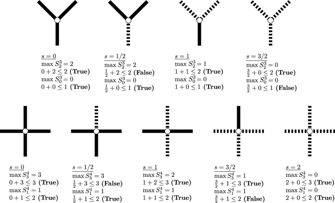
Figure 5: Valid/violating $pq$-inequalities: $s+\max S^{p}_{q}\leq\frac{|p|+|q|-1}{2}$, with $|p|$ and $|q|$ of distinct parities where $q\subset p$. We impose $x^{\prime}_{e}\in\{0,1\}$. The condition characterizing a strong $O$-join can be localized to a neighborhood of a generic $3$-vertex in $V_{12}$. The thick full edges are in $q$ and their set constitutes a strong $O$-join. The coboundary of $v$ is $p$, which is a polygon in $G_{3}$. The dashed edges are the ones in $p\backslash q$. For each half integer $s$ one of its $pq$-inequalities is violated. If $s$ is integer all its induced $pq$-inequalites are valid. Thus, integer $x^{\prime}_{e}$, $e\in E$, plus $pq$-inequalities imply integer double slackness variables $s_{p}$, $p\in V_{12}$.

Let $p\in V_{12}$ and $q\subset p$ so that $|p|+|q|$ is odd. The $pq$-inequality is

$$s_{p}+\sum\{x_{e}:e\subset q\subset p\}\leq\frac{|p|+|q|-1}{2}.$$

The following theorem is central in this work.

Theorem 5.2

The $pq$-inequalities eliminate fractional double slack variables $s_{p}$ in the sense that after including them, integer $x_{e}^{\prime},e^{\prime}\in E$ imply integer $s_{p},p\in V_{12}$.

Proof.    Let $S^{p}_{q}=\sum\{x_{e}^{\prime}:e\subset q\subset p\}$. The analysis for (0-1)-integers $x_{e}^{\prime}$ given in Fig. 5 shows that the vertices with a fractional $s_{p}$ are precisely the ones that violate some restriction. The neighborhood of a vertex in $V_{12}$. The thick edges have $x_{e}^{\prime}=1$ and the dashed edges have $x_{e}^{\prime}=0$. The whole coboundary of the vertex is the edge set of a polygon $p\in G_{3}$.

      □

By simply adding the $pq$-inequalities provides another linear model for the MinStrongOjoin problem:

$P_{1}^{\prime}=\left\{\begin{array}[]{ll}p\in V_{12}:&2s_{p}+\sum\{x_{e}^{\prime}:e\subseteq p\}=|p|\\ q\subset p\in V_{12}:&s_{p}+\sum\{x_{e}^{\prime}:e\subset q\subset p\}\leq\frac{|p|+|q|-1}{2}\\ \rm{bounds:}&0\leq x_{e}^{\prime}\leq 1,s_{p}\geq 0.\end{array}\right.$

Since integrality of $x_{e}^{\prime}$ imply integrality of the $s_{p}$ and each of these appears once in an equation, we can dispose of these double slackness variables variables by considering its implicit definition,

$$s_{p}(integer):=\frac{|p|-\sum\{x_{e}^{\prime}:e\subseteq p\}}{2}{\rm\ \ we\ obtain},$$

$P_{2}^{\prime}=\left\{\begin{array}[]{ll}q\subset p\in V_{12},|p|-|q|{\rm\ odd\ }:&|p|-\sum\{x_{e}^{\prime}:e\subseteq p\}+\sum\{2x_{e}^{\prime}:e\subset q\subset p\}\leq|p|+|q|-1\\ \rm{bounds:}&0\leq x_{e}^{\prime}\leq 1\hskip 8.53581pt\forall e\in E.\end{array}\right.$

Consider $q\subset p\in V_{12}$, $|p|-|q|$ odd:

$$|p|-\sum\{x_{e}^{\prime}:e\subseteq p\}+\sum\{2x_{e}^{\prime}:e\subset q\subset p\}\leq|p|+|q|-1$$

$$\Longleftrightarrow|p|-\sum\{x_{e}^{\prime}:e\subset p\backslash q\}-\sum\{x_{e}^{\prime}:e\subseteq q\subset p\}+\sum\{2x_{e}^{\prime}:e\subset q\subset p\}\leq|p|+|q|-1$$

$$\Longleftrightarrow\sum\{x_{e}^{\prime}:e\subseteq q\subset p\}-\sum\{x_{e}^{\prime}:e\subset p\backslash q\}\leq|q|-1.$$

Theorem 5.3

The polytope

$P_{2}^{\prime}=\left\{\begin{array}[]{ll}q\subset p\in V_{12},|p|-|q|{\rm\ odd}:&\sum\{x_{e}^{\prime}:e\subset q\subset p\}-\sum\{x_{e}^{\prime}:e\subset p\backslash q\}\leq|q|-1\\ \rm{bounds:}&0\leq x_{e}^{\prime}\leq 1\hskip 8.53581pt\forall e\in E.\end{array}\right.$

is a linear model for the MinStrongOjoin problem.

Proof.    It is straightforward from the equivalences above.

      □

We want to get a linear model for the MaxCut problem. Given $P_{2}^{\prime}$ it is enough to replace each variable $x_{e}^{\prime}$ by $x_{e}=1-x_{e}^{\prime}$. This has the effect of complementing the characteristic vectors and the minimization problem becomes a maximization one. We get

$$\sum\{x_{e}^{\prime}:e\subseteq q\subset p\}-\sum\{x_{e}^{\prime}:e\subset p\backslash q\}\leq|q|-1$$

$$\Longleftrightarrow\sum\{1-x_{e}:e\subseteq q\subset p\}-\sum\{1-x_{e}:e\subset p\backslash q\}\leq|q|-1$$

$$\Longleftrightarrow|q|-\sum\{x_{e}:e\subseteq q\subset p\}-(|p|-|q|)+\sum\{x_{e}:e\subset p\backslash q\}\leq|q|-1$$

$$\Longleftrightarrow\sum\{x_{e}:e\subset p\backslash q\}-\sum\{x_{e}:e\subseteq q\subset p\}\leq|p|-|q|-1$$

$$\Longleftrightarrow\sum\{x_{e}:e\subset p\backslash q\}-\sum\{x_{e}:e\subseteq q\subset p\}\leq|p|-p^{-}-1$$

$$\Longleftrightarrow\sum\{x_{e}:e\subset p\backslash q\}-\sum\{x_{e}:e\subseteq q\subset p\}\leq p^{+}-1.$$

Sign of an edge in a polygon. Edges in $p\backslash q$ have sign +1 and edges in $q$ have sign -1. Let $\sigma^{e}_{p}$ be the sign of edge $e$ in polygon $p$. Let $p^{+}$ and $p^{-}$ denote respectively the number of $+1$ signs and $-1$ signs on the edge variables of the polygon $p$. Note that $|p|-|q|$ odd $\Rightarrow$ $|p|-p^{-}$ odd $\Rightarrow p^{+}$ odd. Then the last equivalence can be rewritten as

$$\sum\{\sigma^{e}_{p}x_{e}:e\subset p\}\leq p^{+}-1.$$

Let $S^{\pm}_{12}$ denote the polygons in $V_{12}$ arbitrarily signed except for the fact that $p^{+}$ is odd. Note that we have disposed the $q$’s by using signed polygons. In the Theorem below the linear restrictions forming the polytope are induced by signed forms of the coboundaries of the vertices and the signed forms of the boundary of the faces of map $G_{1}=Pog_{h}\hookrightarrow\mathbb{RP}^{2}$. The phial graph of $G_{1}$ is $G_{3}=K_{z},z=4h$, embedded into some higher genus surface $S^{23}$, which does not concern us except for the practical fact that $G_{3}=K_{z}\hookrightarrow S^{23}$ via shaded rozigs is the easier way to obtain combinatorially the graphs $G_{1}=Pog_{h}$ and its dual $G_{2}$ in $\mathbb{RP}^{2}$ so that $G_{1},G_{2},G_{3}$ have the same edge set $E$.

Theorem 5.4

The polytope

$\mathbb{P}_{12}=\left\{\begin{array}[]{ll}p\in S^{\pm}_{12}:&\sum\{\sigma^{e}_{p}x_{e}:e\subset p\}\leq p^{+}-1\\ \rm{bounds:}&x_{e}\geq 0\hskip 8.53581pt\forall e\in E.\end{array}\right.$

is a linear model for the MaxCut problem on the complete graph $K_{z},z$ even.

Proof.    It is straightforward from the equivalences above, except for the unitary upper bounds. Given any $ij\in E$ there is in $G_{1}$ in a coboundary of a vertex or the boundary of a face of degree 3 or 4 containing $ij$. The variables correspond to unoriented edges. So we have $x_{ij}=x_{ji}$ for every pair of distinct vertices of $G_{3}=K_{z}$.

Case 3. In the first case there is a $k$ so that $x_{ij}+x_{jk}+x_{ki}\leq 2$ and $x_{ij}-x_{jk}-x_{ki}\leq 0$. Adding these, $2x_{ij}\leq 2$ or $x_{ij}\leq 1$.

Case 4. If $ij$ is in the coboundary of a vertex or in the boundary of a face of degree 4, there are $k$ and $l$ so that $x_{ij}-x_{jk}-x_{kl}-x_{li}\leq 0,\hskip 5.69054ptx_{ij}+x_{jk}+x_{kl}-x_{li}\leq 2\hskip 5.69054pt.$ Adding we get $2x_{ij}-2x_{li}\leq 2$ or $x_{ij}-x_{li}\leq 1.$ We also have $x_{ij}+x_{jk}-x_{kl}+x_{li}\leq 2,\hskip 5.69054ptx_{ij}-x_{jk}+x_{kl}+x_{li}\leq 2\hskip 5.69054pt.$ Adding we get $2x_{ij}+2x_{li}\leq 4$ or $x_{ij}+x_{li}\leq 2.$ The inequalities imply that $2x_{ij}\leq 3$ and, since $x_{ij}$ is an integer, $x_{ij}\leq 1$.

      □

Estimating $|S^{\pm}_{12}|$. For this estimation we count the number of 3-vertices, 4-vertices, 3-faces and 4-faces of $G_{1}$. If $h$ is an integer, then the number of 3-vertices is $z=4h$ and the number of 3-faces is 0. The number of 4-vertices of $G_{1}$ is $z(h-1)$. The number of 4-faces is $z(h-1)+z/2$. If $h$ is a half integer, then the number of 3-vertices is 0, the number of 3-faces is $z=4h$. The number of 4-vertices is $\lfloor h\rfloor z$. The number of 4-faces is $(\lfloor h\rfloor-1)z+z/2$.

Unifier of vertices and faces. Let a unifier be either a vertex or a face or $G_{1}$. If $h$ is integer the number of $3$-unifiers is $z$ and the number of 4-unifiers is $z(h-1)+z(h-1)+z/2=2z(h-1)+z/2$. If $h$ is a half integer, then the number of 3-unifiers is $z$ and he number of 4-unifiers is $\lfloor h\rfloor z+(\lfloor h\rfloor-1)z+z/2=2\lfloor h\rfloor z-z/2$.

Cardinality of $S_{12}^{\pm}$ in terms of unifiers. This cardinality is 4 times the number of $3$-unifiers plus 8 times the number of 4-unifiers of $G_{1}$. Thus, if $h$ is an integer, the $|S_{12}^{\pm}|$ is $4z+8(2z(h-1)+z/2)=8z+16zh-16z=16zh-8z\leq 16zh=4z^{2}.$ If $h$ is a half integer, then $|S_{12}^{\pm}|$ is $4z+8(2\lfloor h\rfloor z-z/2)=16\lfloor h\rfloor z\leq 16zh=4z^{2}$. Thus, in every case, $|S_{12}^{\pm}|\leq 4z^{2}=O(|E|).$ In fact we have $4z^{2}\leq 10|E|=5z^{2}-5z\Longleftrightarrow 5z\leq z^{2}$ $\Longleftrightarrow z\geq 5,$ which is clearly true, since there is no use in working with $K_{4}$.

Theorem 5.5

The number of linear inequalities defining $P_{2}$ is at most $11|E|$. Each of them involves the sum of no more than 4 edge variables with $\pm 1$ coefficients. The right hand side of them is either 0, 1 or 2.

Proof.    We have established in the above discussion that $|S_{12}^{\pm}|\leq 10|E|$. There are $|E|$ inequalities corresponding to the non-negativity of the variables. The bounds on each inequality are directly seen to hold. So the result follows.

      □

6 Conclusion

The first author acknowledges the partial financial support of CNPq-Brazil, process number 302353/2014-3. The second author acknowledges the financial support of FACEPE, IBPG-1295-1.03/12. In a companion paper the authors show how to use Theorem 5.4 to improve considerably the running time of the IP-solver SCIP ([1, 2]), working in the same MaxCut Problem, using the $\mathbb{P}_{12}$-model. Moreover each solution provided by our algorithm ([7]) is exact and could be polynomially verifiable (polynomial in terms of the number of leaves in the set of SSS-trees). This acronym accounts for Sufficient Search Space Trees, a special set of trees). These trees organize the computation and provide a proof that a solution is complete and correct. In fact we use it to verify a solution produced by the solver. There is also, due to the simplicity of the model, a number of interesting questions currently under investigation, involving theoretical and applied issues.

References

- [1] Tobias Achterberg. Scip – a framework to integrate constraint and mixed integer programming. Technical report, 2004.
- [2] Gerald Gamrath, Tobias Fischer, Tristan Gally, Ambros M. Gleixner, Gregor Hendel, Thorsten Koch, Stephen J. Maher, Matthias Miltenberger, Benjamin Müller, Marc E. Pfetsch, Christian Puchert, Daniel Rehfeldt, Sebastian Schenker, Robert Schwarz, Felipe Serrano, Yuji Shinano, Stefan Vigerske, Dieter Weninger, Michael Winkler, Jonas T. Witt, and Jakob Witzig. The scip optimization suite 3.2. Technical Report 15-60, ZIB, Takustr.7, 14195 Berlin, 2016.
- [3] M.R. Garey and D.S. Johnson. Computers and intractability. Freeman San Francisco, 1979.
- [4] M.X. Goemans and D.P. Williamson. Improved Approximation Algorithms for Maximum Cut and Satisfiability Problems Using Semidefinite Programming. Journal of the Association for Computing Machinery, 1995.
- [5] S. Lins. Graphs of maps, Available in the arXiv as math.CO/0305058. PhD thesis, University of Waterloo, 1980.
- [6] S. Lins. Graph encoded maps. Journal of Combinatorial Theory, Series B, 32:171–181, 1982.
- [7] S. Lins and D. Henriques. The SSS-Algorithm: an exact verifiable algorithm for the MaxCut Problem, in Preparation. 2016.