Reconstructing Links in Directed Networks from Noisy Dynamics

Abstract

In this Letter, we address the longstanding challenge of how to reconstruct links in directed networks from measurements, and present a general method that makes use of a noise-induced relation between network structure and both the time-lagged covariance of measurements taken at two different times and the covariance of measurements taken at the same time. For coupling functions that have additional properties, we can further reconstruct the weights of the links.

The study of networks Strogatz ; AlbertBarabasi ; Newman has emerged in many branches of science. Many systems of interest consist of a large number of components that interact with each other. These systems can be represented as networks with the individual components being the nodes or vertices and the interactions between two nodes being the links or edges that join the nodes. The network structure depicting how the nodes are linked is a crucial piece of information for us to understand the behavior and function of the system that the network represents. It is often difficult to directly measure the network structure while the dynamics of individual nodes can be measured with relative ease. This leads to the interesting question of how to reconstruct the links of a network from the measurements of the nodes. For most systems of interest, one node can affect the dynamics of another node but its own dynamics is unaffected by the latter. These systems are represented as directed networks with directional links. In general, the strength of interaction can be different so the links have different weights.

Most existing reconstruction methods apply only for undirected networks in which interactions between two nodes are mutual. A commonly employed idea is to infer links from correlation of measurements, with a higher correlation interpreted as a higher probability of a link StuartScience2003 ; BrainPRL . For undirected networks with certain forms of diffusive coupling, it has been shown noise ; PRE ; PRErapid that information of the network structure is contained in the inverse of the covariance matrix and not the covariance matrix itself. This explains why systems can be strongly coupled but have weak pairwise correlation weak . Other reconstruction methods either assume the dynamics to be linear YeungPNAS ; SauerPRE or require additional information such as knowledge about nodal dynamics Yu ; Shandilya ; Levnajic ; Consensus ; SciRep2014 and response dynamics to specific perturbations Timme . A number of techniques have been proposed for the detection of directional coupling from time series measurements but these techniques have limitations, particularly when applied to real-world problems Smirnov2005 ; Smirnov2007 . Reconstructing links of directed networks from measurements remains a big challenge Timme0 ; TimmeReview .

In this Letter, we present a general method that reconstruct links in a directed network subject to noise. We show that information of the network structure is contained in a noise-induced relation between the time-lagged covariance of measurements taken at two different times and the covariance of measurements taken at the same time. For coupling functions that have additional properties, we can further reconstruct the weights or relative coupling strength of the links.

We study a network of $N$ nodes and each node is described by a state variable $x_{i}(t)$, $i=1,2,\ldots,N$. The dynamics of the nodes are governed by

$$\frac{d{x}_{i}}{dt}=f_{i}(x_{i})+\sum_{j\neq i}g_{ij}A_{ij}h(x_{i},x_{j})+\eta_{i}\ ,\ \$$ (1)

where $f_{i}$ describes the intrinsic dynamics of node $i$ and $A_{ij}$ are the elements of the adjacency matrix $A$. When the dynamics of node $i$ is affected by node $j$ via the coupling function $h(x_{i},x_{j})$ with strength $g_{ij}$, $A_{ij}=1$ and a link joins node $j$ to node $i$. Otherwise $A_{ij}=g_{ij}=0$. The coupling function satisfies $h_{y}(x,y)\equiv\partial h(x,y)/\partial y\neq 0$ and $h_{y}>0$ thus excitatory and inhibitory links have $g_{ij}>0$ and $g_{ij}<0$ respectively. We consider directed networks such that $A_{ij}$ and $g_{ij}$ are generally asymmetric. We assume no self-interaction so $A_{ii}\equiv 0$. External disturbance acting on node $i$ is modeled by a Gaussian white noise $\eta_{i}$ of zero mean and $\overline{\eta_{i}(t)\eta_{j}(t^{\prime})}=\sigma_{i}^{2}\delta_{ij}\delta(t-t^{\prime})$. The overbar denotes ensemble average over different realizations of the noise.

We consider weak noise so that we can linearize Eq. (1) around its noise-free solution $X_{i}(t)$ to obtain

$$\frac{d}{dt}{\bf\delta x}\approx Q{\bf\delta x}+{\bf\eta}\ ,$$ (2)

where ${\bf\delta x}=(\delta x_{1},\ldots,\delta x_{N})^{T}$ and $\delta x_{i}(t)=x_{i}(t)-X_{i}(t)$ is the deviation of the state variable from the noise-free solution. The superscript $T$ denotes a transpose and the matrix $Q$, whose elements are given by

$$Q_{ij} \equiv g_{ij}A_{ij}h_{y}(X_{i},X_{j})$$ (3)

$$+\left[\sum_{k\neq i}g_{ik}A_{ik}h_{x}(X_{i},X_{k})+f_{i}^{\prime}(X_{i})\right]\delta_{ij}\ ,\ \$$

contains information of the network structure. We define $B(t_{1},t_{2})$ by

$$B(t_{1},t_{2}) \equiv \overline{[{\bf x}(t_{1})-\overline{{\bf x}(t_{1})}][{\bf x}(t_{2})-\overline{{\bf x}(t_{2})}]^{T}}$$ (4)

$$= \overline{[{\bf\delta x}(t_{1})-\overline{{\bf\delta x}(t_{1})}][{\bf\delta x}(t_{2})-\overline{{\bf\delta x}(t_{2})}]^{T}}$$

where the last equality follows because $\overline{X_{i}(t)}=X_{i}(t)$. $B_{ij}(t_{1},t_{2})$ is the covariance of measurements of node $i$ at $t_{1}$ and measurements of node $j$ at time $t_{2}$. We focus on systems that approach a fixed point in the noise-free limit so that $X_{i}$ and thus $Q$ are independent of time. Using Eq. (2), we have Arnold

$$B(t_{1},t_{2}) \approx e^{Qt_{1}}\{\overline{[{\bf\delta x}(0)-\overline{{\bf\delta x}(0)}][{\bf\delta x}(0)-\overline{{\bf\delta x}(0)}]^{T}}\}e^{Q^{T}t_{2}}$$ (5)

$$\ +\int_{0}^{\min(t_{1},t_{2})}e^{Q(t_{1}-t^{\prime})}De^{Q^{T}(t_{2}-t^{\prime})}dt^{\prime}\$$

where $D$ is a diagonal matrix with $D_{ij}=\sigma_{i}^{2}\delta_{ij}$. From Eq. (5), we obtain

$$B(t+\tau,t)\approx e^{\tau Q}B(t,t)\qquad\tau>0\ ,$$ (6)

which is a noise-induced relation between the time-lagged covariance matrix $B(t+\tau,t)$ and the covariance matrix $B(t,t)$. For systems that have stationary dynamics, $B(t+\tau,t)$ depends on $\tau$ only, and can be approximated by (long) time average:

$$B(t+\tau,t)\approx K(\tau)\equiv\langle[{\bf x}(t+\tau)-\langle{\bf x}(t+\tau)\rangle][{\bf x}(t)-\langle{\bf x}(t)\rangle]^{T}\rangle$$ (7)

where $\langle\cdots\rangle$ denotes a time average. Thus we have

$$e^{\tau Q}\approx B(t+\tau,t)B(t,t)^{-1}\approx K(\tau)K(0)^{-1}\equiv e^{\tau M}\ .$$ (8)

It has been shownnoise ; PRE ; PRErapid that the presence of noise leads to a one-to-one correspondence between network structure and the inverse of covariance for undirected networks. Equation (8) is a generalization of such result to directed networks, which relates network structure to both the time-lagged covariance of measurements taken at two different times and covariance of measurements taken at the same time. The matrix $M=\log[K(\tau)K(0)^{-1}]/\tau$ can be calculated from time series measurements of $x_{i}(t)$. Equations (3) and (8) imply

$$M_{ij}\approx g_{ij}A_{ij}h_{y}(X_{i},X_{j})\ ,\qquad i\neq j$$ (9)

hence the off-diagonal elements $M_{ij}$ would separate into different groups depending on whether $A_{ij}=0$ or $A_{ij}=1$ (with $g_{ij}>0$ or $<0$). We identify these different groups of $M_{ij}$ by clustering using Gaussian mixture model note , and, as a result, reconstruct the links of the network.

In SolvingPRE , the authors focussed on the linearized dynamics Eq. (2) and obtained a relation between the “velocity-variable” covariance matrix between $dx_{i}/dt$ and $x_{j}(t)$ and the covariance matrix. Their relation is the $\tau\to 0$ limit of Eq. (8). To evaluate the velocity-variable covariance matrix, one needs both $x_{i}(t)$ and $dx_{i}/dt$ but the latter is usually not measured and is difficult to estimate accurately from $x_{i}(t)$. Our method makes use of Eq. (8), which holds for finite $\tau$, to reconstruct $A$ (and not $Q$) of directed networks using solely the measured $x_{i}(t)$.

We test our method using directed and weighted random (DWR) and directed and weighted scale-free (DWSF) networks (Table 1). DWR1 and DWR2 are directed random networks of connection probability 0.2 with DWR2 further restricted to contain only unidirectional links such that $A_{ij}=0$ for $i>j$. For both DWR1 and DWR2, $g_{ij}$’s are taken from a Gaussian distribution $N(10,2)$ of mean 10 and standard deviation 2 and all the links turn out to have $g_{ij}>0$. DWR1s has the same adjacency matrix $A$ as DWR1 but $g_{ij}$’s are taken from a different Gaussian distribution $N(10,10)$ such that the links have both positive and negative $g_{ij}$. DWSF is constructed by converting some bidirectional links of a undirected weighted scale-free network barrat2004 into directional links with the power-law distribution of $g_{ij}$ kept intact and the out-degree $k_{\rm out}(i)=\sum_{j}A_{ij}$ distribution being the same as the original power-law degree distribution. We consider $f_{i}$ given by the logistic function

$$f_{i}(x)=r_{i}x(1-x)$$ (10)

and two coupling functions

$$h^{\rm diff}(x,y) = y-x$$ (11)

$$h^{\rm syn}(x,y) = (1/\beta_{1})\{1+\tanh[\beta_{2}(y-y_{0})]\}\ .$$ (12)

The linear diffusive coupling function $h^{\rm diff}$ is a common model for gap junction coupling while $h^{\rm syn}$ is a generalization PRErapid of a model for synaptic coupling between neurons Siam1990 . The parameters $\beta_{1}$, $\beta_{2}$, and $y_{0}$ are chosen such that the steady-state values $X_{i}$ are close to $y_{0}$.

Network	$N$	$N_{B}$	$N_{U}$	$N_{L}$	$\rho$	$g_{ij}$
DWR1	100	186	1678	2050	0.207	$N(10,2)$
DWR1s	100	186	1678	2050	0.207	$N(10,10)$
DWR2	100	0	1035	1035	0.105	$N(10,2)$
DWSF	1000	3120	3730	9970	0.00998	$P(g_{ij})\sim g_{ij}^{-6.6}$

Table 1: The networks studied. $N_{B}$ and $N_{U}$ are respectively the number of bidirectionally- and unidirectionally-linked pairs of nodes. The number of links $N_{L}$ is given by $2N_{B}+N_{U}$ and the link density $\rho$ is equal to $N_{L}/[N(N-1)]$.

The theoretical basis of our method is given by Eq. (8), which holds for general networked systems whose linearized dynamics around the noise-free solution is described by Eq. (2) with a time-independent $Q$. To investigate the possible applicability of our method beyond such networks, we consider three additional cases: (i) $f_{i}=0$ and $h^{\rm cubic}(x,y)=(y-x)^{3}$, (ii) networks whose nodes have two-dimensional state variables $(x_{i}(t),y_{i}(t))$ described by the nonlinear FitzHugh-Nagumo (FHN) dynamics FHN , which is a common model for neurons,

$$\dot{x_{i}} = (x_{i}-{x_{i}^{3}}/{3}-y_{i})/\epsilon+\displaystyle\sum\limits_{j\neq i}g_{ij}A_{ij}h(x_{i},x_{j})+\eta_{i}\qquad$$ (13)

$$\dot{y_{i}} = x_{i}+\alpha\,$$ (14)

with $\epsilon=0.01$ and (iii) networks whose nodes have three-dimensional state variables $(x_{i}(t),y_{i}(t),z_{i}(t))$ described by the nonlinear Rössler dynamics Rossler :

$$\dot{x}_{i} = -y_{i}-z_{i}+\sum_{j\neq i}g_{ij}A_{ij}h(x_{i},x_{j})+\eta_{i}$$ (15)

$$\dot{y}_{i} = x_{i}+ay_{i}+\sum_{j\neq i}g_{ij}A_{ij}h(y_{i},y_{j})$$ (16)

$$\dot{z}_{i} = b+z_{i}(x_{i}-c)+\sum_{j\neq i}g_{ij}A_{ij}h(z_{i},z_{j})\ \qquad$$ (17)

with $a=b=0.2$ and $c=9$ (for such parameters, the dynamics is chaotic if the nodes are decoupled). In case (i), the noise-free solution is $X_{i}(t)=X_{0}$ thus $h^{\rm cubic}_{y}(X_{i},X_{j})=0$ and hence the linearized dynamics cannot be a good approximation. In case (iii) the noise-free solution depends on time. We integrate the equations of motion using the Euler-Maruyama method, then calculate $K(\tau)$ and $K(0)^{-1}$ from $x_{i}(t)$ with an average over $T_{av}$ to obtain $M$. We use only $x_{i}(t)$ for reconstruction even for cases (ii) and (iii) and take $\tau=5\times 10^{-4}$, which is the same as the sampling interval of $x_{i}(t)$, $\sigma_{i}=1$, and $T_{av}=1000$ unless otherwise stated.

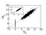
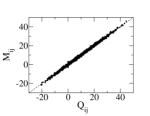
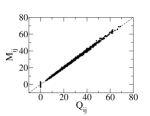
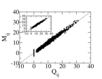
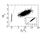
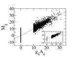
Figure 1: $M_{ij}$ versus $Q_{ij}=g_{ij}A_{ij}h_{y}(X_{i},X_{j})$ or $g_{ij}A_{ij}$ for (a) DWR1 with nonuniform noise (case 2) and inhomogeneous $f_{i}$ (case 3) (inset), (b) DWR1s with both excitatory and inhibitory links (case 5), (c) DWR2 with logistic $f_{i}$ and $h^{\rm syn}$ (case 7), (d) DWSF with logistic $f_{i}$ and $h^{\rm syn}$ with $T_{av}=2000$ (case 9) and $T_{av}=1000$ (inset), (e) DWR1 with $h^{\rm cubic}$ (case 10) and FHN with $h^{\rm syn}$ (case 12, inset), and (f) DWSF with Rössler (case 17) and FHN (case 16, inset) dynamics. See Table 2 for detailed descriptions of the different cases. Dashed line is $y=x$.

We compare the off-diagonal elements of $M$ and $Q$ in Fig. 1. The data points scatter around the line $y=x$, confirming Eq. (9). One cause for the data scatter is due to the finite sample size, the noise generated in our simulations is not exactly delta-correlated in time. [For noise with finite correlation time, Eq. (8) would be modified to $e^{\tau M}\approx e^{\tau Q}+E$ with $M\approx Q$ with an error related to $E$.] This data scatter is reduced when the sample size or $T_{av}$ is increased (see Fig. 1d). For the additional cases (i)-(iii), we compare $M_{ij}$ and $g_{ij}A_{ij}$ and find

$$M_{ij}\approx Cg_{ij}A_{ij}\ ,\qquad i\neq j$$ (18)

for some constant $C$. This interesting result indicates that our method can also be applicable to these cases.

It is common to measure the accuracy of a method by its sensitivity and specificity. However, for sparse networks with link density $\rho\ll 1$, the number of incorrectly inferred links can be substantial leading to a greatly distorted reconstructed network even when specificity is close to 1. So, we measure the accuracy instead by the error rates ${\rm FN}/N_{L}$ and ${\rm FP}/N_{L}$, which are respectively the proportion of the links that are missed (false negatives FN) and the ratio of incorrectly inferred links (false positives FP) to the number of links (see Table 2). Sensitivity is given by $1-{\rm FN}/N_{L}$ while specificity is given by $1-({\rm FP}/N_{L})\rho/(1-\rho)$. The two error rates are less than 10% for all the cases studied (for case 9, the error rates are lowered to less than 10% with a longer $T_{av}=2000$), including network acted upon by nonuniform noise (case 2), network with inhomogeneous intrinsic dynamics (case 3), network with both excitatory and inhibitory links (case 5), and networks with dynamics given by the additional cases (i)-(iii) beyond the description given by Eq. (2) (cases 10-17). From Eq. (9) or the approximate extension Eq. (18), we expect that weak links with small $|g_{ij}|$ are difficult to detect. Indeed all links that are missed are of relatively weak coupling strength. For the cases that have the highest error rates in DWR and DWSF networks respectively, we compare directly the reconstructed in- and out-degree of the nodes, $\hat{k}_{\rm in}$ and $\hat{k}_{\rm out}$ with the actual values. Good agreement is found as shown in Fig. 2. Our method can thus capture the power-law out-degree distribution of DWSF rather well.

Case	Network	Dynamics	${\rm FN}/{N_{L}}$	${\rm FP}/{N_{L}}$	$e_{G}$
1	DWR1	logistic $r_{i}=10$; $h^{\rm diff}$	0	0	5.7
2	DWR1	logistic $r_{i}=10$; $h^{\rm diff}$	0	0.63	6.0
3	DWR1	logistic; $h^{\rm diff}$	0	0	6.0
4	DWR1	logistic $r_{i}=10$; $h^{\rm syn}$	2.98	2.00	14.2
5	DWR1s	logistic $r_{i}=10$; $h^{\rm diff}$	9.32	1.90	9.9
6	DWR2	logistic $r_{i}=50$; $h^{\rm diff}$	0	0	4.3
7	DWR2	logistic $r_{i}=50$; $h^{\rm syn}$	0	3.38	4.5
8	DWSF	logistic $r_{i}=100$; $h^{\rm diff}$	0.50	1.11	6.9
9	DWSF	logistic $r_{i}=100$; $h^{\rm syn}$	0.65	2.84	10.3
10	DWR1	$f_{i}=0$; $h^{\rm cubic}$	4.24	2.78	16.6
11	DWR1	FHN $\alpha=1.05$; $h^{\rm diff}$	0	0	5.7
12	DWR1	FHN $\alpha=2$; $h^{\rm syn}$	0	0	4.9
13	DWR1	Rössler; $h^{\rm diff}$	0	0	6.9
14	DWR2	FHN $\alpha=1.05$; $h^{\rm diff}$	0	0	3.3
15	DWR2	Rössler; $h^{\rm diff}$	0	0.10	5.4
16	DWSF	FHN $\alpha=1.05$; $h^{\rm diff}$	0.32	1.20	5.8
17	DWSF	Rössler; $h^{\rm diff}$	0.35	1.58	6.2

Table 2: Accuracy of our reconstruction as measured by the error rates FN$/N_{L}$ and FP$/N_{L}$ (in %) for the cases studied. Case 2: $\sigma_{i}$ taken from $N(1,0.2)$. Case 3: $r_{i}$ taken from a uniform distribution $U(1,50)$ from 1 to 50. Case 4: $(\beta_{1},\beta_{2},y_{0})=(2,0.5,4)$. Case 7: $(\beta_{1},\beta_{2},y_{0})=(0.1,0.5,4)$. Case 9: $(\beta_{1},\beta_{2},y_{0})=(0.5,0.5,4)$ and $T_{av}=2000$. Case 12:  $(\beta_{1},\beta_{2},y_{0})=(0.1,2,-1)$ and $\sigma_{i}=0.1$. Cases 14 and 16: $\sigma_{i}=0.1$. $e_{G}$ is the average percentage error of the reconstructed relative coupling strength $\hat{G}_{ij}$ or $\hat{G}^{\rm out}_{j}(i)$.

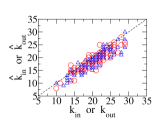
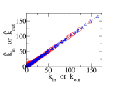
Figure 2: Comparison of the reconstructed in-degrees $\hat{k}_{\rm in}$ (triangles) and out-degrees $\hat{k}_{\rm out}$ (circles) with the actual values for (a) case 5 and (b) case 9.

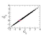
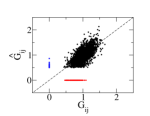
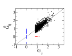
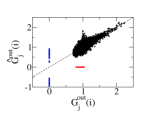
Figure 3: Color online: Comparison of reconstructed $\hat{G}_{ij}$ and $\hat{G}^{\rm out}_{j}(i)$ with the actual values for (a) case 5, (b) case 10, (c) case 17, and (d) case 9. Missed links (red) have $G_{ij}\neq 0$ or ${G}^{\rm out}_{j}(i)\neq 0$ but $\hat{G}_{ij}=0$ or $\hat{G}^{\rm out}_{j}(i)=0$ while incorrectly inferred links (blue) have $G_{ij}=0$ or ${G}^{\rm out}_{j}(i)=0$ but $\hat{G}_{ij}\neq 0$ or $\hat{G}^{\rm out}_{j}(i)\neq 0$. Dashed line is $y=x$.

We define the relative coupling strength of an in- and out-link of node $i$ from and to node $j$ by

$$G^{\rm in}_{j}(i)\equiv\frac{g_{ij}}{\langle g\rangle_{\rm in}(i)}\ ;\qquad G^{\rm out}_{j}(i)\equiv\frac{g_{ji}}{\langle g\rangle_{\rm out}(i)}\$$ (19)

respectively, where $\langle g\rangle_{\rm in}(i)\equiv{\sum_{j}|g_{ij}|A_{ij}}/{k_{\rm in}(i)}$ and $\langle g\rangle_{\rm out}(i)\equiv{\sum_{j}|g_{ji}|A_{ji}}/{k_{\rm out}(i)}$ are the average (absolute) coupling strength of the in- or out-links of node $i$. If $h_{y}(x,y)$ depends on $y$ only as for $h^{\rm syn}$, Eq. (9) implies

$$G^{\rm out}_{j}(i)\approx\frac{M_{ji}\hat{k}_{\rm out}(i)}{\sum_{k\leftarrow i}|M_{ki}|}\equiv\hat{G}^{\rm out}_{j}(i)\ {\rm if}\ h_{y}=h_{y}(y)\ .\$$ (20)

$\sum_{k\leftarrow i}$ represents a sum over nodes $k$ that are reconstructed to be linked from node $i$. Similarly if $h_{y}(x,y)$ depends on $x$ only, we can reconstruct $G^{\rm in}_{j}(i)$ using $\hat{G}^{\rm in}_{j}(i)\equiv{M_{ij}\hat{k}_{\rm in}(i)}/{\sum_{k\rightarrow i}|M_{ik}|}$, where $\sum_{k\rightarrow i}$ represents a sum over nodes $k$ that are reconstructed to link to node $i$. If $h_{y}(x,y)$ is a constant as for $h^{\rm diff}$, Eq. (9) gives

$$G_{ij}\equiv\frac{g_{ij}}{\langle g\rangle}\approx\frac{M_{ij}\hat{k}_{\rm tot}}{{\sum_{n,l\leftrightarrow n}|M_{nl}|}}\equiv\hat{G}_{ij}$$ (21)

where $\langle g\rangle\equiv\sum_{ij}|g_{ij}|A_{ij}/\sum_{ij}A_{ij}$ and $\hat{k}_{\rm tot}=\sum_{i}\hat{k}_{\rm in}(i)=\sum_{i}\hat{k}_{\rm out}(i)$. The extension Eq. (18) implies that Eq. (21) should hold approximately for the additional cases (i)-(iii). In Fig. 3, we compare the reconstructed relative coupling strength $\hat{G}_{ij}$ and $\hat{G}^{\rm out}_{j}(i)$ with the actual values. The average percentage error (excluding missed and incorrectly predicted links) ranges between 3.3% to 17% for all the cases studied (see Table 2).

In conclusion, we have presented a method that reconstructs links in directed networks. Our method makes use of a noise-induced relation Eq. (8) that gives a one-to-one correspondence of the network structure and both the time-lagged covariance and covariance of measurements. Using numerically simulated data, we have shown that our method can successfully reconstruct the network structure with low error rates for DWR and DWSF networks with different nonlinear dynamics and coupling functions. Our method is general and requires only time series measurements of the nodes. For coupling functions that have additional properties, our method can further reconstruct the weights of the links.

- (1) S.H. Strogatz, Exploring complex networks, Nature (London) 410, 268 (2001).
- (2) R. Albert and A.-L. Barabási, Statistical mechanics of complex networks, Rev. Mod. Phys. 74, 48 (2002).
- (3) M.E.J. Newman, The Structure and Function of Complex Networks, SIAM Rev. 45, 167 (2003).
- (4) J.M. Stuart, E. Segal, D. Killer, and S.K. Jim, A gene-coexpression network for global discovery of conserved genetic modules, Science 302, 249 (2003).
- (5) V. M. Eguíluz, D. R. Chialvo, G. A. Cecchi, M. Baliki, and A. V. Apkarian, Scale-Free Brain Functional Networks, Phys. Rev. Lett. 94, 018102 (2005).
- (6) J. Ren, W.-X. Wang, B. Li, and Y.-C. Lai, Noise Bridges Dynamical Correlation and Topology in Coupled Oscillator Networks, Phys. Rev. Lett. 104, 058701 (2010).
- (7) E.S.C. Ching, P.Y. Lai, and C.Y. Leung, Extracting connectivity from dynamics of networks with uniform bidirectional coupling, Phys. Rev. E 88, 042817 (2013); Erratum, Phys. Rev. E 89, 029901(E) (2014).
- (8) E.S.C. Ching, P.Y. Lai, and C.Y. Leung, Reconstructing Weighted Networks from Dynamics, Phys. Rev. E 91, 030801(R) (2015).
- (9) E. Schneidman, M.J. Berry, R. Segev, and W. Bialek, Weak pairwise correlations imply strongly correlated network states in a neural population, Nature 440, 1007 (2006).
- (10) M. K. S. Yeung, J. Tegner, and J. J. Collins, Reverse engineering gene networks using singular value decomposition and robust regression, Proc. Natl. Acad. Sci. U.S.A. 99, 6163 (2002).
- (11) D. Napoletani and T. D. Sauer, Reconstructing the topology of sparsely connected dynamical networks, Phys. Rev. E 77, 026103 (2008).
- (12) D. Yu, M. Righero, and L. Kocarev, Estimating Topology of Networks, Phys. Rev. Lett. 97, 188701 (2006).
- (13) S. G. Shandilya and M. Timme, Inferring network topolgy from complex dynamics, New J. of Phys. 13, 013004 (2011).
- (14) Z. Levnajić and A. Pikovsky, Network Reconstruction from Random Phase Resetting, Phys. Rev. Let. 107, 034101 (2011).
- (15) S. Shahrampour and V. M. Preciado, Reconstruction of Directed Networks from Consensus Dynamics, American Control Conference, 1685 (2013).
- (16) Z. Levnajić and A. Pikovsky, Untangling complex dynamical systems via derivative-variable correlations, Sci. Rep. 4, 5030 (2014).
- (17) M. Timme, Revealing Network Connectivity from Response Dynamics, Phys. Rev. Lett. 98, 224101 (2007).
- (18) D. Smirnov, R. Andrzejak, Detection of weak directional coupling: Phase-dynamics approach versus state-space approach, Phys Rev E 71, 036207 (2005).
- (19) D. Smirnov, B. Schelter, N. Winterhalder, and J. Timmer, Revealing direction of coupling between neuronal oscillators from time series: Phase dynamics modeling versus partial directed coherence, Chaos 17, 013111 (2007).
- (20) M. Timme, Does dynamics reflect topology in directed networks?, Europhys. Lett. 76, 367 (2006).
- (21) M. Timme and J. Casadiego, Revealing networks from dynamics: an introduction, J. Phys. A 47, 343001 (2014).
- (22) L. Arnold, Stochastic Differential Equations: Theory and Applications, John Wiley & Sons (1974).
- (23) We use MATLAB fitgmdist to fit the data by a Gaussian mixture model of 2 components then use MATLAB cluster to obtain the posterior probabilities of each component for each data point. For each data point , if the posterior probability of the component with a mean closest to 0 (which is associated with the component for unconnected nodes) is less than 0.5, then this is inferred to be from connected nodes and . Otherwise, . For DWR networks, clustering analysis is performed on all () values as a whole while for DWSF network, clustering analysis is performed on values for fixed separately for each .
- (24) Z. Zhang, Z. Zheng, H. Niu, Y. Mi, S. Wu, and G. Hu, Solving the inverse problem of noise-driven dynamic networks, Phys. Rev. E 91, 012814 (2015).
- (25) A. Barrat, M. Barthélemy, and A. Vespignani, Weighted Evolving Networks: Coupling Topology and Weight Dynamics, Phys. Rev. Lett. 92, 228701 (2004).
- (26) G.B. Ermentrout and N. Kopell, Oscillator Death in Systems of Coupled Neural Oscillators, SIAM J. Appl. Math. 50, 125 (1990).
- (27) R. FitzHugh, Impulses and Physiological States in Theoretical Models of Nerve Membrane, Biophys. J. 1, 445 (1961).
- (28) O. E. Rössler, An Equation For Continuous Chaos, Phys. Lett. A 57, 397 (1976).