A universal density structure for circum-galactic gas
Abstract
We develop a new method to constrain the physical conditions in the cool () circumgalactic medium (CGM) from measurements of ionic column densities, by assuming that the cool CGM spans a large range of gas densities and that small high-density clouds are hierarchically embedded in large low-density clouds. The new method combines the information available from different sightlines during the photoionization modeling, thus yielding tighter constraints on CGM properties compared to traditional methods which model each sightline individually. Applying this new technique to the COS-Halos survey of low-redshift galaxies, we find that we can reproduce all observed ion columns in all 44 galaxies in the sample, from the low-ions to O vi, with a single universal density structure for the cool CGM. The gas densities span the range ( is the cosmic mean), while the physical size of individual clouds scales as , from of the low density O vi clouds to of the highest density low-ion clouds. The deduced cloud sizes are too small for this density structure to be driven by self-gravity, thus its physical origin is unclear. The implied cool CGM mass within the virial radius is (1% of the halo mass), distributed rather uniformly over the four decades in density. The mean cool gas density profile scales as , where is the distance from the galaxy center. We construct a 3D model of the cool CGM based on our results, which we argue provides a benchmark for the CGM structure in hydrodynamic simulations. Our results can be tested by measuring the coherence scales of different ions.
1. Introduction
Observations of the circumgalactic medium (CGM), defined loosely as gas within the halo virial radius but outside the galaxy main stellar body, can constrain two crucial processes in the formation of galaxies – inflows from the intergalactic medium (IGM) and outflows from the galaxy. The CGM is also a potential site for some of the ‘missing baryons’, which are baryons expected from big bang nucleosynthesis but unaccounted for by observations (Fukugita et al. 1998; Bell et al. 2003). Therefore, estimates of the CGM mass and its physical properties provide important constraints for both theories of galaxy formation, and for the inventory of cosmic baryons.
The mass of the cool () baryons in the CGM, , can be derived from an estimate of the average photoionized hydrogen column through the CGM, via
| (1) | |||||
where is the gas mass per hydrogen particle. A possible approach to estimate the average is to compile a sample of projected galaxy-QSO pairs without any absorption pre-selection. Then for each galaxy, one can measure the ionic column densities along the sightlines to the background quasar, and apply an ionization correction in order to deduce the total column. This approach yields a relatively unbiased census of the gas around galaxies. Recently, Werk et al. (2014) applied this method to the COS-Halos survey of galaxies at redshift (Thom et al. 2012; Werk et al. 2012, 2013; Tumlinson et al. 2013), and found , more than the typical stellar mass in the galaxies in their sample. Additional similar surveys have been undertaken in order to estimate the CGM properties of galaxies with different luminosities and redshifts (Hennawi et al. 2006a; Prochaska & Hennawi 2009; Crighton et al. 2011; Rudie et al. 2012; Prochaska et al. 2013; Bordoloi et al. 2014; Lau et al. 2015).
Most studies of the CGM assume that the absorption features come from gas with some characteristic volume density , and therefore some characteristic ionization level (). However, when is optimized to reproduce the column of low-ionization ions such as Si ii and Si iii, the observed O vi columns are underpredicted by orders of magnitude (e.g. Werk et al. 2014). In some cases, even the column of the lower ionization Si iv is underestimated by the single-density models optimized to fit the low ions (Werk et al. 2016). When higher-ionization ions such as Ne viii are observed, their observed columns are also severely underpredicted by the single- models fit to the low-ions (Savage et al. 2005b; Narayanan et al. 2011; Meiring et al. 2013). These discrepancies suggest that single- models are likely an oversimplification, and have led the authors of these studies to argue for a multi-phase CGM. However, once multiple phases are invoked, our ability to observationally constrain the CGM properties drops considerably, due to the extra free parameters. For example for the high-ion phase, which is typically traced only by O vi since other high-ions such as Ne viii are challenging to observe, both photoionization and collisional ionization have been invoked (e.g. Savage et al. 2002), though neither can be ruled out. This uncertainty in the ionization mechanism results in huge uncertainties in the mass of this phase and hence in the total CGM mass (Tumlinson et al. 2011; Peeples et al. 2014; Werk et al. 2014). Another disadvantage of the multi-phase picture is that it does not naturally explain why the kinematics of O vi and other high ions are commonly found to be aligned with the kinematics of the low-ions (e.g. Simcoe et al. 2002, 2006; Prochaska et al. 2004; Tripp et al. 2011; Fox et al. 2013; Werk et al. 2014; Crighton et al. 2015).
In this paper we introduce a new method to model circumgalactic photoionized gas which spans a range of densities, under the assumption that the different densities are spatially associated as suggested by the line kinematics. Our new method uses absorption line modeling to derive the hydrogen column per decade in density , which is the natural extension of the total column to multi-density gas. We show below that the formalism allows combining information on the density structure from different objects during the absorption line modeling, i.e. it allows one to model the ‘stacked’ CGM of a large ensemble of observations of different galaxies. This stacking yields tight constraints on the properties of the multi-density CGM, compared to traditional methods in which each object is modeled individually, and the aggregate CGM properties are deduced from some average over the individual absorption models.
The quantity , known as the Absorption Measure Distribution (AMD), is the absorption analog of the emission measure distribution (EMD) widely used in the analysis of emission-line spectra. Its importance was recognized in the context of ‘warm absorbers’ – outflowing gas seen as absorption features in X-ray spectra of Active Galactic Nuclei. Analysis of the AMD in these systems was used both to demonstrate the existence of a thermal instability in the absorbing gas, and to constrain the physical conditions in the outflows (Holczer et al. 2007; Blustin et al. 2007; Behar 2009; Holczer & Behar 2012; Stern et al. 2014b; Adhikari et al. 2016; Goosmann et al. 2016). For the CGM, equation (1) suggests that an estimate of yields a constraint on , namely the cool gas mass distribution as a function of gas density. This mass distribution can be directly compared to the predictions of hydrodynamic simulations.
This paper is structured as follows. In §2 we present the formalism we use to analyze a multi-density CGM, and describe our method to derive in a sample of galaxy-selected absorbers. In §3 we apply this method to the COS-Halos sample, while in §4 we use the determined to deduce aggregate characteristics of the CGM of COS-Halos galaxies. We discuss the uncertainties and implications of our results in §5. In §6 we summarize our results and suggest how they can be expanded in future work.
2. Formalism and Method
In this section we provide analytic estimates for the absorption features expected in a multi-density cool CGM, followed by a prescription for calculating a more accurate solution using the numerical photoionization code cloudy (Ferland et al. 2013). The formalism is based on the formalism in Hennawi & Prochaska (2013), who discussed a CGM filled with cool clouds which have the same density and size, and are distributed uniformly within the virial radius . We first generalize the Hennawi & Prochaska formalism to allow a cloud distribution which varies as a function of the distance from the galaxy , and then further generalize to a CGM with clouds with different densities.
2.1. Single-Density Cool Cloud Model
A CGM filled with homogeneous spherical clouds can be characterized using the cloud density , the cloud size , and the volume filling factor . We assume a spherically-symmetric CGM in which varies as a power law in , and is zero beyond :
| (2) |
The above five parameters define this idealized cool CGM model, and can be used to derive aggregate CGM quantities. The cool CGM mass within is (for )
| (3) | |||||
The above five parameters can also be used to calculate quantities which are either directly observable or closely related to absorption line observations. One such quantity is the average column density , where we use the symbol to denote an average over an ensemble of sightlines through the CGM of a galaxy, or an ensemble of sightlines through the CGM of a homogeneous selected sample of galaxies. The value of as a function of impact parameter is related to and via
| (4) |
where is the hydrogen number density, and is the line element. The integral in eqn. (4) is equal to the average pathlength of the sightline through the cool clouds. This integral is further developed in §4 where we constrain from observational data.
A second observable is the covering factor , defined as the chance a line of sight intersects at least one cloud111This is a somewhat different definition then used by Hennawi & Prochaska (2013), who defined as the average number of clouds along the sightline. The two definitions are equivalent if cloud overlap along the sightline is negligible.. The relation between , and is straightforward in the limit that clouds do not overlap along a single line of sight. In this limit, the contribution to per unit length is , where is the cloud number density and is the cloud cross-sectional area. Hence
| (5) |
Using eqns. (4) and (5) to solve for we get
| (6) |
Therefore, in the context of this single-density cloud model one can constrain , and from the observations, and then use equations (4)–(6) to deduce the physical parameters , , and . These parameters can then be used to derive the aggregate characteristics of the CGM.
It is important to note that this formalism allows calculating only average observational quantities, because a single sightline depends on a specific realization of the CGM, and the the resulting stochasticity is not fully specified by the five parameters mentioned above.
2.2. Multi-Density Cool Cloud Model
We now generalize the model from the previous section to CGM clouds which span a range of gas densities. For the analytic formalism we utilize a discrete picture in which CGM clouds can have one of a set of densities , in which consecutive values differ by an order of magnitude, i.e. . We find this discrete picture conceptually and notationally simpler than a more realistic scenario where varies continuously. This discrete picture is also used for visualization purposes. However, for increased accuracy in the numerical photoionization calculation below, we use the finer sampling in used by cloudy, where consecutive values of typically differ by .222cloudy divides the calculated slab into layers, where the depth of each layer is chosen such that the physical conditions are roughly uniform across the layer.
We assume that all clouds with a given density have the same size
| (7) |
where is the lowest density in the cool CGM and . The filling factor of each cloud type is assumed to have the form
| (8) |
i.e. the dependence of on is assumed to be separable from the dependence of on . More complicated forms for are not well-constrained with the COS-Halos sample used below, and are not analyzed in this work.
Using these seven parameters , , , , , , it is straightforward to generalize the equation for the mass within (eqn. 3) to a multi-density CGM:
| (9) |
Another interesting property is the distribution of cool gas mass within as a function of gas density, which is equal to
| (10) |
Similarly, the average column along the sightline (eqn. 4) is generalized in a multi-density CGM to the average AMD, i.e. the average column per decade in density
| (11) |
The covering factor of clouds with density is (in the limit that same- clouds do not overlap along a sightline)
| (12) |
and from eqns. (11)–(12) we get
| (13) |
similar to the expression in the single density model (eqn. 6). In the following section we discuss how and can be constrained from absorption line measurements of ionic column densities.
2.3. Absorption Features in a Multi-Density CGM
What are the ionic columns expected in a multi-density CGM? The column of ion along a given line of sight is equal to
| (14) |
where is the abundance of element relative to hydrogen, assumed for simplicity to be independent of , and is the fraction of at ionization level . We emphasize that eqn. (14) is accurate for a single line-of-sight, not only for an ensemble average. Now, in the absence of self-shielding is primarily a function of the ionization parameter , defined as
| (15) |
where is the ionizing photon flux incident on the cloud. The coefficient in eqn. (15) originates from the choice of normalization, where we normalize by , the cosmic mean baryon density at (equivalently, ), and we normalize by , defined as
| (16) |
In eqn. (16) is the UV background intensity at found by Haardt & Madau (2012, hereafter HM12), the integrand is from the Lyman edge () to infinity, and is the speed of light. The redshift is chosen to match the objects analyzed below.
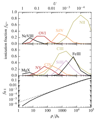
The dependence of on for several ions with ionization potential is shown in Figure 1. The calculations are performed with version 13.03 of cloudy (last described by Ferland et al. 2013) on a slab of gas illuminated by the UV background at calculated by HM12. The gas is assumed to have solar metallicity and a column of , though these two parameters have a small effect on as long as the slab is optically thin at . The effect of deviations from the HM12 UV background are addressed in the discussion. Figure 1 demonstrates that each metal ion exists in significant quantities only within a dynamical range of in , so to first order we can keep only one term in the sum in eqn. (14) for each ion. Assuming for example a CGM composed of three densities , , and , we get
| (17) |
where we replaced with the solar abundance of each element (Asplund et al. 2009) multiplied by the metallicity in solar units . Equation (2.3) demonstrates that the AMD , which is the column density associated with a given density phase, can be directly constrained from observed ion columns given the metallicity (which one also typically fits for).
Eqn. (2.3) also suggests a close relation between the covering factors of the different ions and the covering factor of gas with different densities, i.e. is roughly equal to the chance that a sightline with impact parameter shows O vi absorption, is equal to the chance a sightline shows Si iv absorption, and is equal to the chance a sightline shows N ii absorption.
Thus, absorption line observations combined with photoionization modeling provide constraints on the two observable quantities and , which can then be used to determine the parameters of the multi-density cloud model.
2.4. A Hierarchical Cool CGM
The kinematic alignment of low-ions and high-ions mentioned in the introduction suggests a spatial correlation between the high-density and low-density clouds. Hence, we make an additional assumption on the structure of the multi-density cool CGM, that small high-density clouds are hierarchically embedded in larger low-density clouds. Using the example from the previous section we imagine an idealized case of three gas phases, one tracing O vi, one tracing Si iv, and one tracing N ii, as pictured in the top panel of Figure 2.
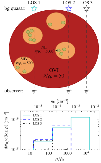
Figure 2 shows three possible lines-of-sight (LOS) through the hierarchical cloud, where LOS 1 intersects gas with all the considered densities, LOS 2 intersects the medium- and low-density gas, and LOS 3 intersects only the low-density gas. We hence expect all three LOSs to exhibit O vi absorption, but only LOS 1 and LOS 2 should exhibit appreciable Si iv absorption, and only LOS 1 to exhibit appreciable N ii. This property of the hierarchical structure that low-ions are always expected to be associated with high-ions, but not vice-versa, is consistent with absorption line observations (see below), and hence supports our assumption of a hierarchy.
The bottom panel of Figure 2 shows the AMDs of the three LOSs pictured in the top panel. The AMDs are calculated from the pathlength of each LOS through each phase, as shown in the Figure, where the assumed scale is such that the O vi-cloud size is . Note that the AMD of LOS 2 is roughly equal to the AMD of LOS 1, truncated at . Similarly, the AMD of LOS 3 is roughly equal to the AMD of LOS 1 truncated at . That is, the AMDs of different LOSs can be considered as segments of some ‘universal’ AMD which spans all , but which are truncated at some maximum density which is specific to the individual LOS. In other words, if the AMD of individual sightlines is a power-law of the form
| (18) |
then all sightlines have roughly the same and , while they differ significantly only in their . Except the truncation, the differences between the three AMDs are small, of order unity. These small differences originate from the different possible pathlengths of a LOS through a given cloud, and from the different number of same- clouds intersected by a LOS.
Our approach to fitting photoionization models to CGM absorption line data is thus as follows. We utilize the standard approach of galaxy-selected samples of CGM absorbers (such as COS-Halos) to treat individual sightlines through the CGM of similar galaxies as different sightlines through the same CGM. We fit the same and to all objects, while the difference between the absorption features in different objects is set by the maximum density encountered along the sightline. We also fit an individual gas metallicity to each object, which is held constant across all phases333The metallicity may in principle depend on gas density, for example in the picture suggested by Schaye et al. (2007). We defer exploring this possibility to future work.. That is, we model the observed absorption features of all objects in the sample simultaneously, using two universal parameters ( and ) plus two parameters per object ( and ). Our approach hence has an advantage over previous studies of galaxy-selected samples of CGM absorbers. While the conventional approach is to model each sightline separately, and then discuss the aggregate CGM properties via some average over these noisy individual absorption models, our approach combines the constraints from all objects during the absorption line modeling itself to obtain one high S/N fit for the model parameters.
Before elaborating on the numerical absorption line modeling in the next section, we provide some physical intuition for the parameters and introduced in eqn. (18). In the hierarchical model is equal to the fraction of sightlines which have :
| (19) |
because the hierarchical assumption implies that a sightline with truncation density intersects all lower density phases. Combining eqn. (19) with eqn. (18) implies that the average AMD of an ensemble of sightlines is equal to
| (20) |
Now, by comparing eqn. (20) with eqn. (13) we get
| (21) |
Since is the average pathlength through a cloud, eqn. (21) implies that equals the average column of a sightline through a single cloud with density . Also, since (eqn. 7) we get
| (22) |
These last two relations are accurate in the no-overlap limit, in which eqn. (13) is derived. When allowing for overlaps of same- clouds along the line of sight, equals the average column in sightlines which intersect at least one cloud with density . So, eqn. (22) overestimates by a factor equal to the mean number of -clouds along such sightlines, which can be estimated numerically.
2.5. Numerical Photoionization Modeling
To derive a more accurate solution of the expected absorption features as a function of , , , and , we use the photoionization code cloudy. Specifically, cloudy allows us to drop the crude approximation in eqn. (2.3) that each ion originates exclusively from a single phase, and also to account for the effects of self-shielding.
cloudy can calculate the ionization structure of a slab where the gas density varies as a function of the H-column measured from the slab surface (note that is a coordinate within the slab, in contrast with which is the total column observed along some line of sight). To find the dependence of on which reproduces a desired AMD, we integrate eqn. (18) ():
| (23) |
which implies
| (24) |
Equivalently, for we get and . In all calculations we set , or equivalently , since layers with are so highly ionized that they do not change the predicted columns of ions observed in the COS-Halos sample analyzed below. Observations of higher ionization lines such as are required to constrain the properties of these low density layers (see Figure 1). Available Ne viii observations are addressed in the discussion. Assuming higher values for yields poorer fits.
In total, we run 168 cloudy models, with or 0.75; , or ; and or 3. For each combination of and , we run cloudy where within the slab varies according to eqn. (24). We assume a HM12 incident spectrum and solar relative abundances in all calculations. The stopping criterion of the models is set to an arbitrary large of . In order to reproduce the truncation of the AMD at as discussed above, for each layer in the slab calculated by cloudy we record the gas density and the column of each ion from the illuminated surface up to this layer. Thus, for each cloudy model with parameters and for each ion , we get a predicted column as a function of , yielding a four-dimensional grid for each ion . To derive for parameters which are not in the grid, we interpolate between the nearest grid values. H i is treated as any other ion in the fit.
For a given sample of quasar-galaxy pairs, we use the Levenberg-Marquardt algorithm (Press et al. 1992) to find the best-fit for all ion columns with free parameters: and for each object, plus one universal and one universal . For comparison, the standard photoionization modeling approach where a constant-density model is fit to each absorber has parameters, namely , and for each object ( is often replaced with ). Similarly, an absorber-specific model which fits two densities per object has parameters (two , two , and one per object).
The likelihood to be maximized is
where is an index over all objects in the sample, is the observed column of ion in object , and curly brackets denote a set of parameters or measurements. This likelihood is similar to the likelihoods in Crighton et al. (2015) and Fumagalli et al. (2016). We assume a common error of on all measurements, larger than the typical measurement uncertainties of . This error accommodates expected variations in of order 50% between different sightlines, as seen in the lower panel of Figure 2 and further justified below. This error also accommodates for relative abundance deviations from Solar. Note that since a constant error is assumed on all column measurements, the absolute value of the error does not affect the result of the best-fit.
In cases where a measurement is an upper or lower limit, we adopt an approach similar to Crighton et al. (2015) where we assume a one-sided Gaussian with error beyond the limit. If the predicted column conforms to the limit then the argument of the sum in eqn. (2.5) is assumed to be zero. Since is basically a chi-square except for how we treat limits, for ease of notation we henceforth use .
2.6. The relation between and
Another noteworthy property of the hierarchical model is the close relation between and . This relation can be derived by noting that the H i fraction can be approximated as (bottom panel of Figure 1)
| (26) |
where in the second equality we assume . Using eqn. (26) in eqn. (18) we get that the contribution to from each phase is
| (27) |
Eqn. (27) implies that for the value of is determined by the gas with the highest density along the line of sight, i.e.
| (28) |
If we assume and , which are close to the best-fit values found below, we get
| (29) | |||||
where we replaced with the expression in eqn. (26). Eqn. (29) suggests that the large dynamical range of in observed in the COS-Halos sample (Tumlinson et al. 2013) is due to a similarly large dynamical range in the maximum gas density encountered along the sightline .
3. Application to the COS-Halos sample
3.1. The COS-Halos sample
We use data from the COS-Halos survey (Tumlinson et al. 2011, 2013; Thom et al. 2012; Werk et al. 2012, 2013, 2014) of CGM gas surrounding 44 galaxies at low-redshift () with luminosity . COS-Halos observed 39 UV-bright quasars within an impact parameter from the sample galaxies using the Cosmic Origins Spectrograph (COS; Green et al. 2012) on board the Hubble Space Telescope (HST). Tumlinson et al. (2013) discuss the design and execution of the survey. For our purposes, we use 580 of the 589 metal ion column measurements listed in Werk et al. (2013), including detections and limits of all ions up to O vi, and excluding only the nine measurements which are marked as ‘blended and saturated’. These column measurements were derived using the apparent optical depth method (Savage & Sembach 1991) on a velocity range typically from the galaxy redshift. The 379 non-detections (65%) are given as 2 upper limits, while another 74 absorption features (13%) are saturated, so they are treated as lower limits. In cases where there are multiple detected transitions for a certain ion in a given object, we use the weighted mean ion column listed in Table 3 in Werk et al. (2013).
We supplement the metal ion columns with the 44 H i-column measurements listed in Table 1 of Werk et al. (2014). Four objects have no detection of a Lyman absorption feature, so their are treated as upper limits. In another 22 objects the allowed range of is an order of magnitude or more since the Lyman features are saturated. We treat these measurements as two-sided limits, where the contribution to (eqn. 2.5) is zero if the predicted falls within the allowed range, and an error of is assumed beyond the allowed range. Including these measurements, we fit a total of 624 detections and limits.
3.2. Fit results
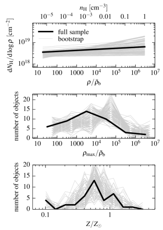
We apply the fitting algorithm described in §2.5 to the 624 column measurements. The best-fit AMD normalization and AMD slope are shown in the top panel of Figure 3. To estimate the error on and we use the bootstrap method, where we choose with replacement objects from the COS-Halos sample and run the fit on this new sample, repeating this process 100 times. The found AMD is
with
| (30) |
and the distribution of shown in the middle panel of Figure 3. The errors on and quoted in eqn. (30) are marginalized errors, since these two parameters are covariant. Note the fit values of span a large dynamical range of . The implications of this distribution are discussed in the next section.
The fit distribution is shown in the bottom panel of Figure 3. The typical in the CGM of COS-Halos galaxies is found to be , with of the objects in the range of . The plotted distribution excludes the four objects in which all ion measurements are upper limits, and therefore cannot be constrained. Four additional objects have only H i detections, and hence the fit of 0.1, 0.1, 0.1, and 0.3 in these objects are upper limits.
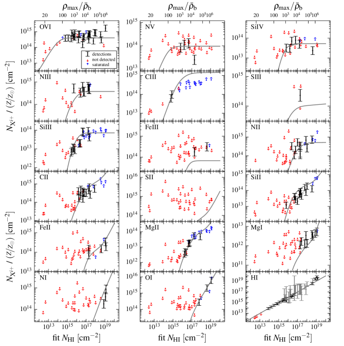
Figure 4 compares the ion columns calculated by our best-fit model to the observed columns. Each of the 18 panels shows a specific ion, where the panels are ordered by decreasing ionization energy. The gray lines are the calculated ion columns as a function of (noted on top), assuming . The fit , which is closely related to (see approximation in eqn. 29), is noted at the bottom of the Figure. The observed ion columns are plotted versus the best-fit (and also ) of the relevant object, and the metal ion columns are normalized by the fit . Detections are marked by error bars with our assumed uncertainty of 0.2 dex (eqn. 2.5), while upper and lower limits are marked by colored arrows. Therefore, each panel in Figure 4 has up to 44 data points, one from each foreground galaxy in the sample.
By eye, the expected and observed ion columns are generally in good agreement. The best-fit yields a maximum likelihood estimate (eqn. 2.5) of , for a sample of data points of which 148 are detections and 476 are limits, using 90 free parameters (a universal and , and and for each of the objects). However, since a large fraction of data points are limits, the model is non-linear and the usual per degree of freedom intuition does not hold (Andrae et al. 2010). Therefore, in the next section we perform an alternative assessment of the goodness-of-fit using the cross-validation technique.
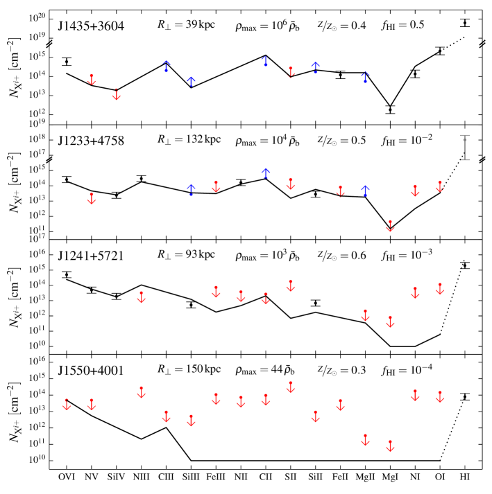
The O vi panel in Figure 4 demonstrates that the predicted increases with increasing only at (), and is independent of at larger values of . This predicted independence of on at large is apparent in the COS-Halos observations, and has also been observed in other samples of intervening absorbers at low (Danforth et al. 2014), and also at (Muzahid et al. 2012; Lehner et al. 2014). In the context of our model, this independence of on occurs since O vi is produced only in the low density layer with (), which the AMD in the upper panel of Figure 3 shows has a characteristic column of . According to eqn. (2.3), this characteristic H-column implies a characteristic (for ), and a characteristic (eqn. 26). The observed will surpass this value of only if the line of sight passes through higher density layers, which have a lower ionization state and hence a larger H i fraction. These layers will not however increase the observed , since oxygen is less than five times ionized within them. Hence, since lines-of-sight which traverse the high-density layers also cross the low density O vi-layer, then for all the expected column is . Thus, the independence of on above some ‘transition-’ is a direct result of our assumption that all the O vi is photoionized and that the density structure of the absorbing gas is hierarchical. The value of this transition- of is set by the typical expected in solar metallicity photoionized gas with where O vi is most efficiently produced.
The trend of increasing at small and independence of on at large , is also apparent in other ions in Figure 4, where the ‘transition-’ increases with decreasing ionization energy. This characteristic behavior has also recently been observed in C iv-absorbers at (Kim et al. 2016). The increase in the transition- with decreasing ionization energy occurs since low-ions reside in high-density layers, which produce a larger . Thus, ions with different ionization energies are created within different parts of the absorber. At , the optical depth to H i-ionizing radiation becomes substantial, and the ionization state of the gas is dominated by the optical depth rather than by the gas density. In these self-shielded regions of the cloud only the column of atoms and ions which are created by photons with energy (e.g. Mg ii) increase with .
Figure 5 compares the calculated and observed ions grouped by object, for a few COS-halos galaxies. From the 40 objects with detections in at least one ion, we show the objects with the highest, 14th-highest, 27th-highest, and lowest , in order to span the entire and range. The fits to the rest of the objects are available online444http://www2.mpia-hd.mpg.de/homes/stern/UniversalFits/. For reference, we note for each object the impact parameter , the best-fit and , and the calculated . As implied by Figure 4, Figure 5 shows that the calculated ion columns are generally consistent with the observations. Figure 5 also demonstrates that as and increase (bottom panel to top panel) lower-ionization ions become more prominent.
The flat AMD slope we find (eqn. 30) implies that the total gas column scales only logarithmically with (eqn. 23). Thus, in the 40 objects with at least one detected absorption feature we find a small dispersion in total column of , despite the large range in . This result is consistent with the result of Prochaska et al. (2004), who deduced in five of six absorbers along the line of sight to PKS 0405-123.
3.3. Comparison with absorber-specific modeling
As can be seen in Figures 4–5 and discussed above, the quality of the fit is reasonable, and explains the general trends in the data, supporting our suggested CGM density structure. However, a quantitative estimate of the goodness-of-fit is not straightforward, since the found depends strongly on our assumed error of , which is somewhat uncertain, and the models are non-linear in the parameters such that the usual per degree of freedom intuition does not hold. Also, we wish to compare the success of our universal model with the absorber-specific models typically used in the literature. For this purpose it is not trivial to use a -like goodness of fit criteria since universal and absorber-specific models differ significantly in the number of free parameters. Therefore, in this section we use the cross-validation technique to compare the predictive power of our universal model with the predictive power of absorber-specific models. In cross-validation, one randomly partitions the data points into a ‘training set’, on which the free parameters of the model are optimized, and then calculates the measure-of-fit (here the score) on the remaining ‘validation set’ using the parameters optimized to fit the training set. This procedure tests the ability of the model to predict unknown data points. The process is repeated several times with different partitions, which yields a distribution of per model. The resulting distributions of of the different models can then be compared to check which model has the strongest predictive power.
We compare our universal model with the following three absorber-specific models. The first model is a constant-density absorber with a single gas density per line of sight. In this model, we find the values of , and which best-fit the observed ion columns in each object, for a total of free parameters. As discussed in the introduction, this method has been shown repeatedly in the past to fail at reproducing the entire set of absorption features in a given object, since when is optimized on the low-ions, O vi is typically underpredicted by orders of magnitude. The standard alternative is to assume a multi-phase absorber, where O vi originates from a second phase with a different . We therefore use cross-validation also on a two-phase model, which has free parameters (, , , , and per object). For these constant-density models, we run cloudy with a constant or . All other cloudy parameters are identical to the power-law model described in §2.5. As above, we create a three-dimensional table of predicted ion columns as a function of , , and . In the two-phase model, the predicted is equal to the sum of the predicted from each phase. The third absorber-specific model assumes a power-law density distribution equivalent to that used above, but where each objects has its own distinct profile, which implies free parameters (, and per object).
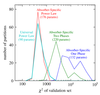
For each cross-validation iteration, we randomly choose 30% of the metal ion columns in each object as the validation set. The free parameters are then optimized by fitting the training set (the other 70% of the measurements), and then the (eqn. 2.5) of the validation set is calculated. A hundred iterations are run for each of the four models, and the -distributions are shown in Figure 6.
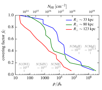
Figure 6 shows that the median of the universal model used in this study is a factor of 20 lower than the median in the absorber-specific constant density model, and a factor of 5 lower than in the absorber-specific two-phase model. The -distributions of the universal and absorber-specific power-law models are comparable. This result implies that the power-law models have stronger predictive power than the traditional single and double density methods used in the literature, and they are therefore favored.
Figure 6 also shows that the distribution of the universal and absorber-specific power-law models are similar. If the density structure across the COS-Halos sample had been perfectly universal, one would expect the distribution of the universal power-law model to be lower than the distribution of the absorber-specific power-law model, since the extra flexibility provided by the unnecessary free parameters in the absorber-specific model reduce its predictive power. In contrast, if the density structure along sightlines in the COS-Halos sample had a large dispersion, the universal model would produce bad fits to the data and therefore would have a higher distribution than the absorber-specific power-law model. The similar distribution of the two power-law models hence suggests that there is some dispersion among the density structure of the different COS-Halos sightlines, though this dispersion is not very large. This dispersion may be connected to the difference in the CGM of star-forming and quiescent galaxies found by Tumlinson et al. (2011), or alternatively to the relatively wide range of impact parameters probed (). This dispersion will be explored in future work.
4. Implied CGM characteristics
In this section we combine the best-fit results of the previous section with the formalism developed in §2 in order to calculate aggregate CGM characteristics.
4.1. Covering Factors
In the context of our hierarchical model, is the highest density encountered along a given line-of-sight, which thus determines the lowest ionization state along the sightline. As such, the covering factor is equal to the chance a sightline with impact parameter has . We therefore divide the sample into three bins in , namely , , and , each with objects555The COS-Halos sample was selected so each of these bins has the same number of objects (Tumlinson et al. 2013).. The implied are shown in Figure 7. The values of drop with increasing (by construction) and with increasing , from of the low-density O vi phase to of the high-density Mg i phase. Note though that the drop in is a weak function of (roughly logarithmic), with dropping by only per decade in .
4.2. Cloud Sizes
We return to the discrete picture where consecutive values of differ by an order of magnitude (). In the appendix we calculate the relation between the fine sampling of in the cloudy calculation used above and the discrete densities used here. The implied lowest density phase in the discrete picture of our best-fit model is (). The best-fit implies that the column of this phase is , where is the minimum density in the cloudy calculation and the best-fit is given by eqn. (30).
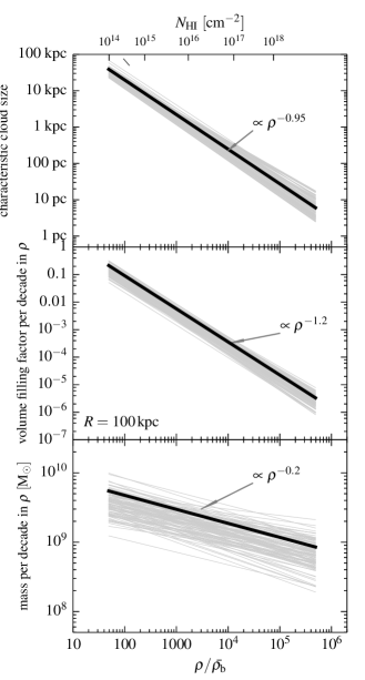
An initial estimate for the size of clouds with different can be obtained from the relations and (eqn. 22), which is accurate in the limit that clouds with the same do not overlap along the line-of-sight. However, as noted above the assumption that same clouds do not overlap is a simplification which over-predicts . Below we show that when accounting for cloud overlap, the implied clouds sizes are a factor of smaller then the sizes estimated in the no-overlap limit. Hence, , and the best-fit and (eqn. 30) imply
| (31) |
This relation is shown in the top panel of Figure 8, which also illustrates the errors implied by the bootstrap errors on and (eqn. 30). The characteristic size of the densest phase found above () is hence , almost four orders of magnitude smaller then the size of the O vi-phase.
4.3. Filling Factor and Mass
The flat AMD found above implies that the cloud size scales roughly as (eqn. 31). In contrast, the covering factor depends only logarithmically on (Figure 7). We can use these two properties to gain intuition on the dependence of the filling factor on , in the context of the hierarchical model where multiple dense clouds are embedded in a larger low-density cloud. Since the cross-sectional area of the cloud scales as , then for the phases and to have the same , each cloud needs to be populated by clouds with density . Since the cloud volume scales as , these 100 clouds fill a fraction of of the parent cloud volume, and have a total gas mass which is roughly equal to the mass of the parent cloud. Hence, the weak dependence of on seen in Figure 7, combined with the flat AMD found above, imply roughly equal CGM mass per decade in , but a filling factor which scales as .
A more accurate calculation of can be derived from eqns. (11) and (20), which together give
| (32) | |||||
Defining as the cosine of the angle between the plane of the sky and a radial vector to a point along the sightline, we get and . Using these geometrical relations in eqn. (32) we get
where we used the power-law form for (eqn. 8), and we set the limits of the integral from the edge of a sphere with to the mid-plane, and multiply by two.
Using least square minimization, we find the , , and which best-fit the observed , , and according to eqn. (4.3). This process yields
| (34) |
For deriving equation (34) we assume , the average virial radius of COS-Halos galaxies (Werk et al. 2014). Eqn. (34) is plotted in the middle panel of Figure 8. This Figure also illustrates the bootstrapped errors in our calculation, where in each bootstrap iteration we choose with replacements 15 objects in each -bin to derive , and choose randomly one of the bootstrapped and shown in the top panel of Figure 3.
We now use eqn. (34) to derive aggregate CGM characteristics. By eqn. (10), the CGM mass in each density phase is
| (35) |
Equation (10) demonstrates that the mass is distributed roughly equally between the different density bins, consistent with our simplified estimate above. Eqn. (35) is plotted in the bottom panel of Figure 8.
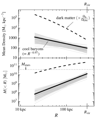
Eqn. (34) also implies that the average density profile of the cool CGM as a function of is
| (36) |
and the total cool gas mass within is (eqn. 9)
| (37) |
These profiles and their bootstrapped errors are shown in Figure 9. The marginalized error on the slope of the profile is , while the implied total mass within the virial radius is
| (38) |
4.4. CGM realization
To provide a visualization of the hierarchical CGM structure derived in this study, we create a realization of the CGM based on the physical parameters and found above. We use the realization also to justify our claim in §4.2 that when accounting for cloud overlap along the line of sight, the implied are lower by a factor of than when are estimated in the no-overlap limit.
We randomly populate a sphere with size with the clouds which have . The number and distribution of the clouds are set to reproduce the value of found above (eqn. 34). We then randomly populate each cloud with clouds, in order to reproduce the desired relative filling factor of the two phases of (eqn. 34), given the cloud volume ratio of (eqn. 31). We assume that clouds are uniformly distributed over the volume occupied by the clouds, which creates a separable dependence of on and on , as assumed in eqn. (8). This recursive populating of clouds is repeated for the , , and phases.
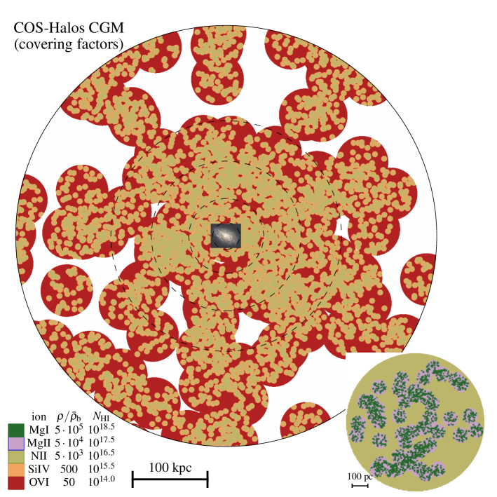
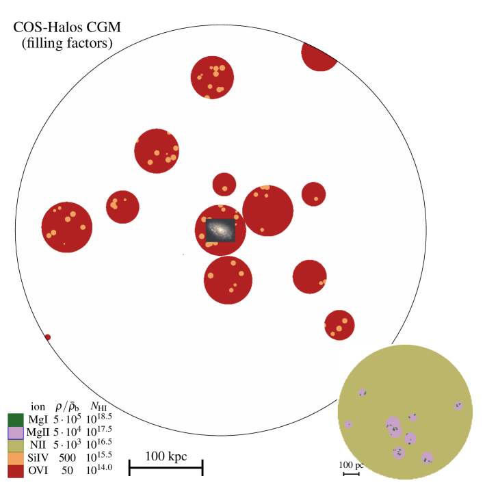
The CGM realization is shown in Figures 10 and 11. Figure 10 shows the projection of the CGM on the plane of the sky, where the plotted color denotes the maximum density observed along each line of sight. This figure depicts the covering factors of the different phases plotted in Figure 7. Figure 11 shows an infinitesimal slice of the CGM through the mid-plane, where color denotes the gas density. This Figure depicts the filling factors of the different phases (eqn. 34). Table 1 lists for each phase the size and mass of single clouds, and the average number of clouds within a cube with edge size .
As discussed in §2.4, eqn. (22) overestimates by a factor equal to the average number of -clouds along sightlines which intersect at least one -cloud. Table 1 lists this factor for each phase, calculated along skewers through the realization that have , the range of probed by the COS-Halos survey. The mean number of clouds are all in the range , within of the factor of used to derive the cloud sizes in eqn. (31), thus justifying the derived sizes. The weak trend in the mean number of clouds with may suggest that low density clouds are somewhat smaller than estimated, while high-density clouds are somewhat larger than estimated. The implied change in the index is however very small, of order .
The dispersion in the number of clouds listed in the right column of Table 1 is approximately in all phases. This dispersion is an estimate for the variance in the gas columns of individual sightlines compared to the universal AMD. This result supports our choice above to assume an error of when comparing the universal model predictions with specific ion columns observed in individual sightlines (eqn. 2.5).
The realization also implies that typically of sightlines which intersect at least one cloud in some phase intersect exactly one cloud of this phase, intersect two clouds of this phase, and intersect three clouds. Assuming that different clouds are offset in velocity space, this result can be tested by investigating the number of distinct kinematic components in absorption spectra. We further discuss cloud kinematics in §5.2.
5. Discussion
| ion | cloud mass | clouds per | clouds(b) | ||
|---|---|---|---|---|---|
| per LOS | |||||
| O vi | |||||
| Si iv | |||||
| N ii | |||||
| Mg ii | |||||
| Mg i |
In this study, we assume a phenomenological model for the CGM, where the cool photoionized gas is composed of small dense clouds which are hierarchically embedded within larger lower-density clouds, with some characteristic relation between physical scale and gas density. We develop a method to combine (or ‘stack’) the observations from all 44 COS-Halos objects, and thus yield tight constraints on the density structure. This universal phenomenological model produces an acceptable fit to all observed ions, including both the low-ions and the high-ions up to O vi (Figures 4–5), and has both higher predictive power and fewer parameters than the standard models used in the literature (Figure 6). In this section, we discuss some of the uncertainties in our analysis, the implications and predictions of our derived quantities, and how our results can be compared to hydrodynamical simulations.
5.1. Uncertainty in the ionizing spectrum
As shown in Figure 1, the ionization fractions of the different ions are sensitive to , the ratio of the ionizing photon flux to the gas density. Therefore, the range of densities of derived above depends (linearly) on the assumed . We assume above the value of found by HM12, which is based on the luminosity function of quasars at , and assuming that the contribution from star forming galaxies (and other sources) is negligible. However, recently Kollmeier et al. (2014) compared low- Ly forest observations with cosmological simulations, and found that the required is higher by a factor of than HM12 synthesized by summing the emission from all sources of ionizing photons. The quantitative value of this discrepancy, however, has been contested by follow-up studies, which found a weaker discrepancy of a factor of (Shull et al. 2015; Heilker, private communication). The uncertainty in propagates to our derived , e.g. if we assume , than the implied CGM density range is increased by a factor of five to .
Also, since the observations constrain the column densities , than any uncertainty in propagates to an uncertainty in . Therefore, assuming a Kollmeier et al. UVB implies that the characteristic size of the O vi-phase is , rather than the derived above (eqn. 31). Reversing the argument, then if we had an independent estimate of the cloud sizes, say by measuring the ion coherence scale (see below), our results would provide a constraint on .
On the other hand, the derived CGM mass estimates do not depend on the assumed . This follows since (eqn. 9), and is proportional to (eqn. 11). The CGM mass is essentially an integration of the observed columns over the CGM cross-section (eqn. 1). Since the hydrogen columns are derived from the observed ionic columns after ionization corrections (eqn. 14), and the ionization corrections are independent of the absolute density scale which is set by , the CGM mass is hence also independent of .
Another potential source of ionizing photons is star formation (SF) in the local galaxy (Miralda-Escudé 2005; Schaye 2006). To estimate the contribution of local SF to the ionizing spectrum we follow Kannan et al. (2014), who assumed the SED of a old stellar population and an escape fraction of (black curve in fig. 1 there). The ratio of photons from the galaxy to the HM12 UV background at is hence
| (39) |
where the median star formation rate (SFR) in the COS-Halos sample is (Werk et al. 2013). Bearing in mind the high uncertainty in , eqn. (39) suggests a significant contribution to the ionizing flux from local SF, especially in blue galaxies and at low . A significant contribution from the local galaxy would both decrease the implied size of the absorbers as discussed above, and imply a mean cool gas density profile steeper than the found in Fig. 9.
The ionizing spectrum may also have a different shape then calculated by HM12, for example a softer spectrum is expected if SF in the galaxy dominates the photon budget. A different spectral shape implies that the ion fractions peak at different than shown in Figure 1, which will affect the derived density structure. We estimate the effect of a different spectral shape by recalculating Fig. 1 with a hard ionizing spectrum (, where ) and a soft ionizing spectrum (). For comparison, the spectral slope in HM12 is roughly . The peak of O vi is shifted by a factor of to lower values in the hard spectrum, and by a factor of to higher values in the soft spectrum. The peak of lower-ions are shifted by a smaller amount, where the shift generally decreases with decreasing ionization energy, as expected. A factor of change in the peak implies a factor of change in the implied and also in the implied cloud size. However, this change is small compared to the range of in deduced above, suggesting that the uncertainty in the spectral shape does affect our conclusion that the cool CGM spans a large range in gas density.
5.2. Implications for the velocity field
Figure 11 in Werk et al. (2013) plots the ion absorption profiles seen in 14 COS-Halos objects with detections in both high-ionization and low-ionization lines. The mean velocities of the highly-ionized metal ions are roughly aligned with the mean velocities of low-ionized metal-ions, while the high-ions tend to have broader and smoother profiles than the low-ions. As mentioned in the introduction, these absorption profile characteristics are commonly seen in CGM absorbers. A common interpretation is that the high-ions originate from a higher temperature collisionally-ionized phase which resides at the interface of the cool low-ion clouds with an external medium (hence the kinematic alignment, e.g. Simcoe et al. 2002, 2006; Savage et al. 2005a; Tripp et al. 2008, 2011; Kwak et al. 2011; Fox et al. 2013; Lehner et al. 2014; Crighton et al. 2015). However, the behavior of the absorption profiles is also consistent with (and are a primary motivation for) the hierarchical model presented in this study. Assuming some smooth velocity field in the halo which is dominated by non-thermal motions, then a large high-ion cloud will span some portion of it, which will set the shape of the high-ion absorption profile. A low-ion cloud embedded in the high-ion cloud will span some portion of the velocity field spanned by the high-ion parent cloud. Hence, we expect the kinematics of the low-ion clouds to be some ‘fraction’ of the kinematics of the high-ion parent cloud. In other words, the spatial hierarchy assumed in this study implies also a kinematic hierarchy, which means that the low-ion absorption profiles should be roughly aligned and narrower than the high-ion profiles, as observed.
In cases where the line of sight traverses several low-ion clouds (up to three are expected in a typical sightline, see §4.4), we expect the low-ion absorption profiles to occupy different locations (in velocity space) within the O vi absorption profile, as is indeed seen in J1016+4706 (fig. 11 in Werk et al. 2013).
A possible challenge for the hierarchical model is the tight kinematic correspondence between low- and intermediate-ions (e.g. Si iii vs. Si ii, C iii vs. C ii) noted by Werk et al. (2013). In the hierarchical model these ions are not entirely co-spatial, and hence the kinematic alignment should not be perfect. We defer a thorough analysis of the velocity profiles of the ions in the context of the hierarchical model to future work.
The expected H i profile in our picture is somewhat more complex, since the kinematically-broad O vi clouds are associated with a characteristic of , while the kinematically-narrow low-ion clouds are associated with larger . Therefore, the total H i profile should appear as the sum of these different components. A possible test of the model is using lines of sight with , which should intersect an O vi cloud but no low-ion clouds. In this case, there should be no confusion with H i absorption from the low-ion phases, and the H i absorption should originate from the O vi-absorbing gas. Since in our photoionized picture the temperature is low () even in the O vi-phase, the contribution of thermal broadening to the total broadening is small, and compared to the median in the COS-Halos sample. Hence, along sightlines we expect the H i velocity profile to be similar to the velocity profile of O vi.
5.3. The ionization mechanism of O vi
As discussed in the introduction, the question whether O vi absorption originates in photoionized or collisionally-ionized gas has important implications for the physical conditions in galaxy halos. This question has been addressed by numerous studies using both observational and theoretical arguments (Heckman et al. 2002; Fox et al. 2007; Thom & Chen 2008; Tripp et al. 2008; Howk et al. 2009; Wakker & Savage 2009; Oppenheimer & Davé 2009; Savage et al. 2010, 2011a, 2011b, 2012, 2014; Narayanan et al. 2010a, b, 2011, 2012; Prochaska et al. 2011; Fox 2011; Bordoloi et al. 2016; Gutcke et al. 2016; Oppenheimer et al. 2016; Fielding et al. 2016). In this work we assume O vi originates in the lowest-density phase of the photoionized hierarchical structure (Figs. 10-11). To allow for the possibility that O vi originates instead in collisionally-ionized gas, we refit the free parameters in our model using all COS-Halos data excluding O vi and N v. We find , , and , consistent with the results found above (eqn. 30) when the measured O vi and N v columns are included in the fit . Thus, if O vi originates in collisionally-ionized gas, then the cool CGM picture we derive for the mid- and low-ions remains intact, and one must only exclude the lowest-density phase (i.e., the red circles in Figs. 10-11).
We note that the success of our fit provides a challenge for scenarios where O vi is collisionally-ionized. Since we derive the same best-fit parameters when we exclude the O vi measurements, our model essentially predicts the typical O vi column based on the typical columns of the mid- and low-ions. That is, in our model where density is a smoothly varying parameter, the higher density phases connect smoothly via our two-parameter density profile to the low-density phase probed by OVI. If OVI is actually collisionally ionized, then the ability of our model to explain OVI so well is a peculiar coincidence.
Additionally, the photoionized scenario predicts the minimun associated with O vi detections. This follows since in our model O vi originates from gas with in which is maximized (Fig. 1). In these conditions, , which for the deduced and the typical observed implies . The O vi-panel in Fig. 4 shows that the COS-Halos observations are consistent with this prediction – all objects with O vi detections have and all six objects with are not detected in O vi. Again, any scenario where O vi is collisionally ionized needs to reproduce this relation between and .
Another argument invoked to support the collisionally-ionized scenario for O vi is that the line width increases with , as expected in a cooling flow where O vi is collisionally-ionized (Heckman et al. 2002; Sembach et al. 2003; Fox 2011; Bordoloi et al. 2016). We note that the vs. trend is also qualitatively expected in the cool CGM picture presented in this work. Since the O vi pathlengths of tens of kpc deduced above (Table 1) are a significant fraction of the halo size (), larger suggest a larger pathlength which samples a larger fraction of the halo gravitational velocity field. Hence, an O vi feature with large is expected to have also a large , as observed. We defer a quantitative comparison between the observed vs. relation and our model to future work.
Based on the detection of broad Ly absorbers (BLAs), Savage et al. (2014, hereafter S14) found that of O vi absorbers in a blind low- have , suggesting O vi originates in warm collisionally ionized gas, rather than in cool photoionized gas as assumed here. As noted by S14, this conclusion depends on the assumption that the BLA and O vi absorption arise in the same gas, while in principle BLAs could also arise in cool gas with large non-thermal broadening which is unassociated with O vi (see also Tepper-García et al. 2012). Mass considerations suggest the conditions deduced for the objects in S14 are unlikely to be applicable to COS-Halos objects. The median in these objects is (table 4 in S14). Given the found nearly ubiquitously out to in blue, COS-Halos-like galaxies (Johnson et al. 2015), this implies an O vi-gas mass of (eqn. 1). This mass is larger than the entire baryonic budget of of a blue COS-Halos galaxy, which is unlikely.
5.4. Prediction for the ion coherence scale
A prominent feature of the results of our modeling is the large dynamical range of sizes spanned by CGM clouds, from the O vi-clouds to the size of the densest phase which produces Mg i (top panel of Figure 8, Figures 10–11). Multiple previous studies have already noted that low-ion CGM clouds have sizes of 10s–100s of pc (Rauch et al. 1999; Prochaska 1999; Petitjean et al. 2000; Rigby et al. 2002; Simcoe et al. 2006; Schaye et al. 2007; Prochaska & Hennawi 2009; Rogerson & Hall 2012; Stocke et al. 2013; Werk et al. 2014; Crighton et al. 2015; Lau et al. 2015), thus our results are consistent with these previous results, and extend them by deducing also the larger sizes of the mid- and high-ion clouds.
A testable quantitative prediction of the relation between density and size (eqn. 31) is the coherence scale of each ion. Given two lines of sight with some transverse separation, we expect ions which originate from clouds larger than the transverse separation to show a similar absorption profile in both lines of sight, while ions with sizes smaller than the transverse separation to differ in their absorption profile. Furthermore, since in our picture small dense clouds are grouped within larger low density clouds, some degree of coherence is expected even at transverse separations larger than the characteristic size associated with the ion, though this coherence should not be perfect, and should decrease with increasing separation.
The coherence scale can be measured with observations of absorption systems along multiple sightlines with small transverse separations. Such sightline pairs are available in samples of gravitationally lensed quasars, in which the transverse separations range from 10 down to 10 near the redshift of the source where the light paths converge (Rauch et al. 1999, 2001, 2002; Churchill et al. 2003; Ellison et al. 2004; Lopez et al. 2007; Chen et al. 2014). These studies have deduced a CGM picture consistent with that found here, with kpc O vi clouds (Lopez et al. 2007), kpc C iv clouds (Rauch et al. 2001; Ellison et al. 2004; Lopez et al. 2007), and 100 low-ionization clouds (Rauch et al. 1999, 2002; Churchill et al. 2003). Larger transverse separations can be probed with samples of binary quasars and projected pairs (Hennawi et al. 2006b, 2010; Rorai et al. 2013; Rubin et al. 2015), and were suggested as a similar probe of the coherence length of Lyman-Limit Systems (Fumagalli et al. 2014). A more detailed comparison between our model and coherence scale measurements is deferred to future work.
5.5. A possible Ne viii phase
As mentioned in §2.5, assuming an initial density in the cloudy calculation which is lower than the assumed does not affect the best-fit, since the additional layer of gas is so highly ionized that the contribution to all COS-Halos ions is negligible. Therefore, based on the COS-Halos observations alone we cannot exclude or detect a photoionized gas phase with . Such a phase can in principle exist at where the volume filling factor of all phases discussed above are significantly less than unity (eqn. 34).
This phase could however be detected via its Ne viii or Mg x absorption, which exist in appreciable quantities in gas with (see Figure 1). By extending the best-fit AMD (eqn. 30) to we can derive the expected Ne viii column from this phase:
| (40) |
Ne viii is detectable with COS at , where it is redshifted to observable wavelengths but is not too high such that most of the flux is absorbed by Lyman-limit systems. This redshift range has been observed by the CASBaH sample (PI: Tripp), of which first results are published in Meiring et al. (2013, hereafter M13). M13 find three absorption systems with , which they attribute to the CGM of galaxies, similar to the COS-Halos sample. The Ne viii columns that they find are , , and . A few additional Ne viii systems with similar columns were previously detected by Savage et al. (2005b), Narayanan et al. (2009, 2011) and Hussain et al. (2015). The observed columns are all within a factor of of the value predicted by eqn. (40). Therefore, the photoionized gas model deduced in this work predicts the observed Ne viii column to within a factor of a few. This success may imply that Ne viii originates from low-density photoionized gas.
What are the properties of the Ne viii phase, if it is photoionized as suggested by the extrapolation of our model to lower density? Since the ionization fraction of a given ion depends on , the relation between ionization fraction and depicted in Figure 1 depends on the evolution of the quantity with . Shull et al. (2012) showed that at , which combined with implies is 60% larger at than at . Therefore, for a HM12 background Ne viii at traces gas with . The implied characteristic size of the Ne viii phase at is hence (eqn. 21)
| (41) |
where we used and . Given that our Ne viii column predictions underestimate the observed columns by a factor of , may also be underpredicted by a factor of two, implying that , i.e. the Ne viii phase fills most of the halo of galaxies. Note that the size derived in eqn. (41) is significantly lower than 11 Mpc, the pathlength estimated by Savage et al. (2005b) by assuming Ne viii is photoionized. The difference is mainly because Savage et al. required the observed to originate in the same gas as Ne viii. In our hierarchical model the Ne viii-gas has and (Fig. 1), which implies . The larger observed originates in denser gas.
To conclude this section, extrapolating our model to lower density suggests that the halos of galaxies at are filled with gas (the temperature of photoionized gas with ), which is metal-enriched and has a density eight times the cosmic mean. The expected Ne viii absorption from this phase is consistent with the observations of M13. Hence if NeVIII is indeed photoionized according to our model, then NeVIII absorption systems trace the largest metal enriched regions around galaxies at gas densities comparable to those in the IGM. We note though that if the UV background intensity is stronger than calculated by HM12, as discussed in §5.1, than the density traced by Ne viii is correspondingly larger, and is correspondingly smaller.
5.6. CGM mass
In equation (38), we derive a total cool gas mass within the virial radius of . For comparison, Werk et al. (2014, hereafter W14) measured the photoionized gas mass in COS-Halos galaxies and found , with a lower limit of . The difference between the mass estimate here and in W14 is further enhanced by the fact that here we include the O vi-phase, which accounts for 40% of the total mass (, eqn. 35), while the W14 estimate does not include the O vi-phase.
The higher gas mass is due to the higher ionization-corrected deduced by W14. The difference in the columns deduced by W14 likely reflect the difference between modeling absorption line data with a constant density model as done by W14, compared to modeling using a multi-density absorber as done here. In a multi-density model each ion originates mainly from gas in which peaks, and hence the required gas column required to produce the observed is minimal. In contrast, in a single-density model will inevitably be below-maximal for some of the ions, and hence the fit will tend to deduce larger . The higher predictive power of the power-law models compared to the constant-density models (Figure 6) suggests that CGM absorbers are indeed multi-density.
We also note that the statistical uncertainty in the estimate of found here is substantially lower than the factor of 3 uncertainty deduced by W14. The major source of uncertainty in the W14 analysis is the unknown H i column of objects where the Lyman features are saturated, which compose half of the COS-Halos sample. In the constant-density models used by W14, an unknown implies that and are degenerate, since the expected metal columns are roughly proportional to both properties, while there is no independent estimate of the hydrogen column that can break the degeneracy. Hence, (and ) are not tightly constrained in these objects. In the universal power-law model however, for a given AMD the value of depends only on (eqn. 29), which in turn sets the lowest ionization level expected in the absorber (see Figure 4). Since the universal AMD is constrained by all objects, one can calculate the expected in a given object directly from the lowest-ionization metal ions seen in the absorber, i.e. from the fit . Hence, in these objects there is no degeneracy between and , which propagates to a substantially lower uncertainty in the mass estimate. Thus, the significantly lower uncertainty on derived in this work compared to previous estimates demonstrates the advantage of using our modeling technique for CGM absorbers.
The estimate of found in this work suggests that within , the cool gas mass is only of the typical stellar disk mass of in COS-Halos galaxies (Werk et al. 2012). Adding an unobserved phase, as suggested by observations of Ne viii (§5.5), will increase by (eqn. 35) to half the stellar disk mass. Thus, our results suggest that including the cool CGM baryons does not significantly change the total baryon content of the galaxy.
Figure 9 compares the cool gas density and mass profiles (eqns. 36–37) with the profiles implied by multiplying the dark matter profile (Navarro et al. 1997) by the cosmic baryon mass fraction of . The dark matter profile is calculated assuming , the median halo mass in the COS-Halos sample (Werk et al. 2014), and a concentration parameter of (Dutton & Macciò 2014). The top panel demonstrates that the cool baryon density profile we find is significantly flatter than the dark matter profile at CGM scales. The bottom panel shows that within , the cool CGM baryons account for only 5% of the total baryon budget of .
Figure 9 demonstrates that increases quadratically with , which may suggest the existence of a significant baryon reservoir at . This possibility can be tested by applying our methodology to samples of galaxy-quasar pairs with larger impact parameters than in COS-Halos galaxies, such as Johnson et al. (2015).
5.7. What physical process gives rise to the cool CGM density structure?
Above we find a range of in , from the O vi phase up to the low-ion phase. Since in our model all the gas is photoionized, the gas temperature decreases only mildly with increasing density, from in the O vi phase down to in the densest phase. The thermal pressure of the dense clouds is hence times larger than the thermal pressure of the O vi clouds. In this section we compare the deduced density structure with several simple hydrostatic solutions, and show that they are all unsatisfactory. It is therefore likely that the density structure originates from a hydrodynamic process, the nature of which is currently an open question.
5.7.1 Confinement by hot gas
While the different phases are clearly not in thermal pressure equilibrium, the outer O vi phase may in principle be in pressure equilibrium with an external hot gas phase. In the picture of Mo & Miralda-Escude (1996) and Maller & Bullock (2004), the hot gas is at the virial temperature () and has an over-density that follows the dark matter over-density ( at for the profile shown in Figure 9). Such a scenario has recently been analyzed analytically by Faerman et al. (2016). For the O vi phase to be in pressure equilibrium with this hot phase, the O vi density needs to have a density of . This estimate is a factor of higher than the density of the O vi phase deduced here, significantly larger than the factor of a few uncertainty in due to the uncertainty in the ionizing background (§5.1). This discrepancy is even larger at smaller where the dark matter over-density is higher (Figure 9). Hence if the O vi phase is photoionized as our model suggests, it is unlikely that that the O vi-phase is in pressure equilibrium with such a hot gas phase.
5.7.2 Self-gravity
Gravity balances pressure at the Jeans scale, hence if the CGM clouds are self-gravitating we expect a cloud size of (Schaye 2001)
| (42) |
where is the ratio of gas mass to the total gravitating mass (gas, dark matter and stars). Note that eqn. (42) is derived assuming a constant density cloud, while in our picture each parent cloud is populated by higher-density clouds. However, for the mass distribution deduced above where the mass of embedded clouds is roughly equal to the mass of the parent cloud (§4.3), the implied correction to is small. For , implied by eqn. (42) are larger than the values of derived in eqn. (31), by an order of magnitude for the O vi-phase, and by three orders of magnitude for the densest phase (), ruling out self-gravity with . Alternatively, setting and solving eqn. (42) for gives
| (43) |
For the gas mass deduced above for each phase (lower panel of Figure 8, eqn. 35), the values of in eqn. (43) imply a total gravitating mass of for the O vi phase, and significantly larger gravitating masses for the denser phases. Given the expected total halo mass of , self-gravity is hence ruled out for all phases denser then the O vi phase, and is possible for the O vi phase only if all the halo mass is in the space occupied by the O vi clouds, which is unlikely. A similar conclusion was reached by Simcoe et al. (2006) and Schaye et al. (2007) based on the size they deduced for (single phase) high- absorbers.
Self-gravity is also disfavored for the dense phases since the required number of mini-halos exceeds the number of mini-halos predicted in cosmological simulations (Tumlinson et al. 2013).
5.7.3 Radiation Pressure Confinement
Another potential quasi-static solution which produces a density gradient within the absorber is radiation pressure confinement (RPC), where the gas pressure is in equilibrium with the pressure of the absorbed radiation:
| (44) |
where is the flux density and is the optical depth. RPC conditions have been shown to apply in at least some star forming regions (Draine 2011; Yeh & Matzner 2012; Yeh et al. 2013; Verdolini et al. 2013), in AGN emission line regions (Dopita et al. 2002; Baskin et al. 2014a; Stern et al. 2014a, 2016), in AGN absorption line regions (Stern et al. 2014b; Baskin et al. 2014b), and possibly in the CGM of quasar hosts, in the part exposed to the quasar radiation (Arrigoni Battaia et al. 2016). Assuming that dust grains are embedded in the CGM gas, as suggested by the results of Ménard et al. (2010), then the dominant contribution to the integral in eqn. (44) comes from photons emitted by the galaxy which are absorbed by the grains. Therefore,
| (45) |
where is the dust cross section per H-atom at . For a Galactic grain mixture and dust-to-gas ratio we get
which falls short by an order of magnitude even for the lowest densities found above (). Hence, radiation pressure is too weak to produce the density structure deduced above.
5.8. Comparison with Hydrodynamical Simulations
Our derived CGM density distribution can be compared to theoretical predictions of hydrodynamical simulations of halos at . The simplest approach would be to compare the deduced filling factors (, eqn. 34) and mass distribution (, eqn. 35) with the same parameters in the simulation.
One can also compare the predictions of the simulations with our deduced AMD (, eqn. 30) and covering factor distribution (Figure 7), which are the properties we deduce that include the minimal set of assumptions. To perform such a comparison, one should draw skewers through halos at impact parameters , isolate the photoionized gas (), and record along each pixel of the skewer. Then, for each decade in and for each , calculate the average AMD and covering factor in the different skewers. According to eqn. (20), the ratio of these two values is equal to , and hence the calculated ratio can be compared to the and found here (top panel of Figure 3 and eqn. 30).
We note that it is currently challenging for hydro simulations to resolve the dense CGM phases, as discussed in the context of single-phase absorbers in Crighton et al. (2015, §5.3 there). Zoomed in SPH simulations such as ERIS2 (Shen et al. 2013) and FIRE (Hopkins et al. 2014) have a particle mass of and , respectively. According to Table 1, this particle mass is larger than the masses of single clouds in the two densest phases. If we further apply the requirement of a few thousand particles per cloud in order to resolve hydrodynamic instabilities (Agertz et al. 2007; Crighton et al. 2015), than the third-densest phase is also not resolvable with current simulations. These three phases make up a third of the total cool gas mass (eqn. 35). Similar considerations apply to adaptive mesh refinement simulations which typically have high resolution in the highest density regions in the galaxy disk, but not in the CGM.
6. Summary and Future Work
In this study we develop a new method to analyze ionic column densities measured in the CGM, assuming that the cool () photoionized CGM spans a large dynamical range in gas density, and that the small high-density clouds are hierarchically embedded in larger low-density clouds. Our new method utilizes the formalism of the Absorption Measure Distribution (AMD), defined as the gas column per decade in gas density , which was originally developed for the analysis of ‘warm absorbers’ near AGN. We demonstrate that this formalism allows combining (or ‘stacking’) the information available from different objects during the absorption line modeling, thus yielding significantly tighter constraints on CGM properties compared to traditional analysis methods which model each object individually.
We apply our new method to the COS-Halos sample of low-redshift galaxies, and find the following:
-
1.
The 624 ionic column measurements and limits in all 44 COS-Halos sightlines, from the low-ions (e.g. Mg ii, O i) to O vi, can all be fit with a single normalization and slope of the AMD, namely . The AMD spans the density range , where is the cosmic mean baryon density and is a maximum density fit separately to each object. This success of our new fitting method supports our assumption that the CGM density structure is hierarchical. We use cross-validation to demonstrate that the new fitting method is superior to traditional constant-density methods used in the literature, in terms of its ability to predict unseen data.
-
2.
Our fit provides of each sightline in the sample, which can be used to infer the covering factor of gas as a function of . The covering factor decreases roughly logarithmically with increasing , from for to for .
-
3.
Our results suggest that , i.e. a roughly equal cool CGM mass per decade in . The total mass is , a factor of five lower than estimates based on constant-density modeling. The derived is only 5% of , the cosmic baryon budget of an galaxy.
-
4.
Since , where is the characteristic size of clouds with density , the flat slope of the AMD implies that scales as . This scaling implies that clouds in the CGM span a large dynamical range in size, from of the low density O vi-phase to of the densest phase. This result can be tested by measuring the coherence scale of different ions with multiple sightlines towards lensed and binary quasars.
-
5.
Based on the fit distribution as a function of impact parameter, we find an average cool baryon density profile of at , where is the radial distance from the galaxy center. The uncertainty on the index of the profile is . This profile is significantly flatter than the dark matter profile at the same scales.
-
6.
Extrapolating the best-fit down to correctly predicts the Ne viii column observed in the CGM of galaxies at , which may suggest that Ne viii absorption also originates in photoionized gas.
-
7.
The large range in densities found here coupled with the small range in temperature of photoionized gas () together imply that the gas pressure increases strongly with density. Self-gravity and radiation pressure are too weak to establish this pressure gradient. The nature of the physical mechanism which generates the deduced density structure is currently an open question.
The results of this work can be expanded to find the dependence of the cool gas density structure on galaxy star-formation rate, by applying the methodology independently to the 29 star forming galaxies and 15 quiescent galaxies in the COS-Halos sample. The low detection rate of in red galaxies compared to the high detection rate in blue galaxies (Tumlinson et al. 2011) might suggest that the two galaxy types differ in their cool gas density structure, although our results suggest these differences are not huge given the overall success of the universal fit. If the CGM of more massive quiescent galaxies is filled with a hot () shock-heated gas phase, which is weak or absent in less massive star-forming galaxies (see e.g. Birnboim & Dekel 2003; Kereš et al. 2005; Dekel & Birnboim 2006), then the high pressure from the hot plasma could compress the lowest density cool gas clouds, effectively suppressing the gas required to produce O vi (see §5.7.1). We will explore this interesting possibility in future work.
Our analysis can also be expanded to study the density structure of low-mass halos and halos at high redshift, by applying the same methodology to the COS-Dwarfs sample of low-luminosity galaxies (Bordoloi et al. 2014), and to galaxy-selected absorption samples at (e.g. Hennawi et al. 2006a; Crighton et al. 2011; Rudie et al. 2012; Lau et al. 2015). Additional constraints can be deduced from analyzing absorption-selected samples such as KODIAQ (O’Meara et al. 2015) and CASBaH (Meiring et al. 2013) in the context of the hierarchical picture, under the assumption that these absorbers are associated with galaxies.
Further constraints on CGM properties and tests of our results can be derived from analyzing the gas kinematics in the context of the hierarchical picture (§5.2), and from measurements of the coherence scale of different ions using sightlines with small transverse separations (§5.4). These are all important topics for future work.
References
- Adhikari et al. (2016) Adhikari, T. P., Rozanska, A., Sobolewska, M., & Czerny, B. 2016, arXiv:1601.06726
- Agertz et al. (2007) Agertz, O., Moore, B., Stadel, J., et al. 2007, MNRAS, 380, 963
- Andrae et al. (2010) Andrae, R., Schulze-Hartung, T., & Melchior, P. 2010, arXiv:1012.3754
- Arrigoni Battaia et al. (2016) Arrigoni Battaia, F., Hennawi, J. F., Cantalupo, S., & Prochaska, J. X. 2016, arXiv:1604.02942
- Asplund et al. (2009) Asplund, M., Grevesse, N., Sauval, A. J., & Scott, P. 2009, ARA&A, 47, 481
- Baskin et al. (2014a) Baskin, A., Laor, A., & Stern, J. 2014a, MNRAS, 438, 604
- Baskin et al. (2014b) Baskin, A., Laor, A., & Stern, J. 2014b, MNRAS, 445, 3025
- Behar (2009) Behar, E. 2009, ApJ, 703, 1346
- Bell et al. (2003) Bell, E. F., McIntosh, D. H., Katz, N., & Weinberg, M. D. 2003, ApJ, 585, L117
- Birnboim & Dekel (2003) Birnboim, Y., & Dekel, A. 2003, MNRAS, 345, 349
- Blustin et al. (2007) Blustin, A. J., Kriss, G. A., Holczer, T., et al. 2007, A&A, 466, 107
- Bordoloi et al. (2014) Bordoloi, R., et al. 2014, ApJ, 796, 136
- Bordoloi et al. (2016) Bordoloi, R., Heckman, T. M., & Norman, C. A. 2016, arXiv:1605.07187
- Chen et al. (2014) Chen, H.-W., Gauthier, J.-R., Sharon, K., et al. 2014, MNRAS, 438, 1435
- Churchill et al. (2003) Churchill, C. W., Mellon, R. R., Charlton, J. C., & Vogt, S. S. 2003, ApJ, 593, 203
- Crighton et al. (2011) Crighton, N. H. M., Bielby, R., Shanks, T., et al. 2011, MNRAS, 414, 28
- Crighton et al. (2015) Crighton, N. H. M., Hennawi, J. F., Simcoe, R. A., et al. 2015, MNRAS, 446, 18
- Danforth et al. (2014) Danforth, C. W., Keeney, B. A., Tilton, E. M., et al. 2014, arXiv:1402.2655
- Davé et al. (2010) Davé, R., Oppenheimer, B. D., Katz, N., Kollmeier, J. A., & Weinberg, D. H. 2010, MNRAS, 408, 2051
- Dekel & Birnboim (2006) Dekel, A., & Birnboim, Y. 2006, MNRAS, 368, 2
- Dopita et al. (2002) Dopita, M. A., Groves, B. A., Sutherland, R. S., Binette, L., & Cecil, G. 2002, ApJ, 572, 753
- Draine (2011) Draine, B. T. 2011, ApJ, 732, 100
- Dutton & Macciò (2014) Dutton, A. A., & Macciò, A. V. 2014, MNRAS, 441, 3359
- Ellison et al. (2004) Ellison, S. L., et al. 2004, A&A, 414, 79
- Faerman et al. (2016) Faerman, Y., Sternberg, A., & McKee, C. F. 2016, arXiv:1602.00689
- Ferland et al. (2013) Ferland, G. J., Porter, R. L., van Hoof, P. A. M., et al. 2013a, Rev. Mexicana Astron. Astrofis., 49, 137
- Fielding et al. (2016) Fielding, D., Quataert, E., McCourt, M., & Thompson, T. A. 2016, arXiv:1606.06734
- Fox et al. (2007) Fox, A. J., Petitjean, P., Ledoux, C., & Srianand, R. 2007, A&A, 465, 171
- Fox (2011) Fox, A. J. 2011, ApJ, 730, 58
- Fox et al. (2013) Fox, A. J., Lehner, N., Tumlinson, J., et al. 2013, ApJ, 778, 187
- Fukugita et al. (1998) Fukugita, M., Hogan, C. J., & Peebles, P. J. E. 1998, ApJ, 503, 518
- Fumagalli et al. (2011) Fumagalli, M., Prochaska, J. X., Kasen, D., et al. 2011, MNRAS, 418, 1796
- Fumagalli et al. (2014) Fumagalli, M., Hennawi, J. F., Prochaska, J. X., et al. 2014, ApJ, 780, 74
- Fumagalli et al. (2016) Fumagalli, M., O’Meara, J. M., & Prochaska, J. X. 2016, MNRAS, 455, 4100
- Goosmann et al. (2016) Goosmann, R. W., Holczer, T., Mouchet, M., et al. 2016, arXiv:1603.01448
- Green et al. (2012) Green, J. C., Froning, C. S., Osterman, S., et al. 2012, ApJ, 744, 60
- Gutcke et al. (2016) Gutcke, T. A., Stinson, G. S., Macciò, A. V., Wang, L., & Dutton, A. A. 2016, arXiv:1602.06956
- Haardt & Madau (2012) Haardt, F., & Madau, P. 2012, ApJ, 746, 125 (HM12)
- Heckman et al. (2002) Heckman, T. M., Norman, C. A., Strickland, D. K., & Sembach, K. R. 2002, ApJ, 577, 691
- Hennawi et al. (2006a) Hennawi, J. F., Prochaska, J. X., Burles, S., et al. 2006a, ApJ, 651, 61
- Hennawi et al. (2006b) Hennawi, J. F., Strauss, M. A., Oguri, M., et al. 2006b, AJ, 131, 1
- Hennawi et al. (2010) Hennawi, J. F., Myers, A. D., Shen, Y., et al. 2010, ApJ, 719, 1672
- Hennawi & Prochaska (2013) Hennawi, J. F., & Prochaska, J. X. 2013, ApJ, 766, 58
- Hussain et al. (2015) Hussain, T., Muzahid, S., Narayanan, A., et al. 2015, MNRAS, 446, 2444
- Holczer et al. (2007) Holczer, T., Behar, E., & Kaspi, S. 2007, ApJ, 663, 799
- Holczer & Behar (2012) Holczer, T., & Behar, E. 2012, ApJ, 747, 71
- Hopkins et al. (2014) Hopkins, P. F., Kereš, D., Oñorbe, J., et al. 2014, MNRAS, 445, 581
- Howk et al. (2009) Howk, J. C., et al. 2009, MNRAS, 396, 1875
- Hussain et al. (2015) Hussain, T., Muzahid, S., Narayanan, A., et al. 2015, MNRAS, 446, 2444
- Kannan et al. (2014) Kannan, R., et al. 2014, MNRAS, 437, 2882
- Kereš et al. (2005) Kereš, D., Katz, N., Weinberg, D. H., & Davé, R. 2005, MNRAS, 363, 2
- Kim et al. (2016) Kim, T.-S., Carswell, R. F., Mongardi, C., et al. 2016, arXiv:1601.04660
- Kwak et al. (2011) Kwak, K., Henley, D. B., & Shelton, R. L. 2011, ApJ, 739, 30
- Johnson et al. (2015) Johnson, S. D., Chen, H.-W., & Mulchaey, J. S. 2015, MNRAS, 449, 3263
- Kollmeier et al. (2014) Kollmeier, J. A., Weinberg, D. H., Oppenheimer, B. D., et al. 2014, ApJ, 789, L32
- Lau et al. (2015) Lau, M. W., Prochaska, J. X., & Hennawi, J. F. 2015, arXiv:1510.06018
- Lehner et al. (2013) Lehner, N., Howk, J. C., Tripp, T. M., et al. 2013, ApJ, 770, 138
- Lehner et al. (2014) Lehner, N., O’Meara, J. M., Fox, A. J., et al. 2014, ApJ, 788, 119
- Lopez et al. (2007) Lopez, S., et al. 2007, A&A, 469, 61
- Meiring et al. (2013) Meiring, J. D., Tripp, T. M., Werk, J. K., et al. 2013, ApJ, 767, 49
- Maller & Bullock (2004) Maller, A. H., & Bullock, J. S. 2004, MNRAS, 355, 694 & Zagursky, M. J. 2010, ApJ, 708, L14
- Ménard et al. (2010) Ménard, B., Scranton, R., Fukugita, M., & Richards, G. 2010, MNRAS, 405, 1025
- Miralda-Escudé (2005) Miralda-Escudé, J. 2005, ApJ, 620, L91
- Mo & Miralda-Escude (1996) Mo, H. J., & Miralda-Escude, J. 1996, ApJ, 469, 589
- Muzahid et al. (2012) Muzahid, S., Srianand, R., Bergeron, J., & Petitjean, P. 2012, MNRAS, 421, 446
- Narayanan et al. (2009) Narayanan, A., Wakker, B. P., & Savage, B. D. 2009, ApJ, 703, 74
- Narayanan et al. (2010a) Narayanan, A., Savage, B. D., & Wakker, B. P. 2010a, ApJ, 712, 1443
- Narayanan et al. (2010b) Narayanan, A., et al. 2010b, ApJ, 721, 960
- Narayanan et al. (2011) Narayanan, A., et al. 2011, ApJ, 730, 15
- Narayanan et al. (2012) Narayanan, A., Savage, B. D., & Wakker, B. P. 2012, ApJ, 752, 65
- Navarro et al. (1997) Navarro, J. F., Frenk, C. S., & White, S. D. M. 1997, ApJ, 490, 493
- O’Meara et al. (2015) O’Meara, J. M., Lehner, N., Howk, J. C., et al. 2015, AJ, 150, 111
- Oppenheimer & Davé (2009) Oppenheimer, B. D., & Davé, R. 2009, MNRAS, 395, 1875
- Oppenheimer et al. (2016) Oppenheimer, B. D., Crain, R. A., Schaye, J., et al. 2016, MNRAS,
- Peeples et al. (2014) Peeples, M. S., Werk, J. K., Tumlinson, J., et al. 2014, ApJ, 786, 54
- Petitjean et al. (2000) Petitjean, P., Aracil, B., Srianand, R., & Ibata, R. 2000, A&A, 359, 457
- Press et al. (1992) Press, W. H., Teukolsky, S. A., Vetterling, W. T., & Flannery, B. P. 1992, Cambridge: University Press, —c1992, 2nd ed.,
- Prochaska (1999) Prochaska, J. X. 1999, ApJ, 511, L71
- Prochaska et al. (2004) Prochaska, J. X., Chen, H.-W., Howk, J. C., Weiner, B. J., & Mulchaey, J. 2004, ApJ, 617, 718
- Prochaska & Hennawi (2009) Prochaska, J. X., & Hennawi, J. F. 2009, ApJ, 690, 1558
- Prochaska et al. (2011) Prochaska, J. X., Weiner, B., Chen, H.-W., Mulchaey, J., & Cooksey, K. 2011, ApJ, 740, 91
- Prochaska et al. (2013) Prochaska, J. X., Hennawi, J. F., Lee, K.-G., et al. 2013, ApJ, 776, 136 & Mulchaey, J. S. 2011, ApJS, 193, 28
- Rauch et al. (1999) Rauch, M., Sargent, W. L. W., & Barlow, T. A. 1999, ApJ, 515, 500
- Rauch et al. (2001) Rauch, M., Sargent, W. L. W., & Barlow, T. A. 2001, ApJ, 554, 823
- Rauch et al. (2002) Rauch, M., et al. 2002, ApJ, 576, 45
- Rigby et al. (2002) Rigby, J. R., Charlton, J. C., & Churchill, C. W. 2002, ApJ, 565, 743
- Rogerson & Hall (2012) Rogerson, J. A., & Hall, P. B. 2012, MNRAS, 421, 971
- Rorai et al. (2013) Rorai, A., Hennawi, J. F., & White, M. 2013, ApJ, 775, 81
- Rubin et al. (2015) Rubin, K. H. R., Hennawi, J. F., Prochaska, J. X., et al. 2015, ApJ, 808, 38
- Rudie et al. (2012) Rudie, G. C., Steidel, C. C., Trainor, R. F., et al. 2012, ApJ, 750, 67
- Savage & Sembach (1991) Savage, B. D., & Sembach, K. R. 1991, ApJ, 379, 245
- Savage et al. (2002) Savage, B. D., Sembach, K. R., Tripp, T. M., & Richter, P. 2002, ApJ, 564, 631
- Savage et al. (2005a) Savage, B. D., Wakker, B. P., Fox, A. J., & Sembach, K. R. 2005a, ApJ, 619, 863
- Savage et al. (2005b) Savage, B. D., Lehner, N., Wakker, B. P., Sembach, K. R., & Tripp, T. M. 2005b, ApJ, 626, 776
- Savage et al. (2010) Savage, B. D., et al. 2010, ApJ, 719, 1526
- Savage et al. (2011a) Savage, B. D., Narayanan, A., Lehner, N., & Wakker, B. P. 2011a, ApJ, 731, 14
- Savage et al. (2011b) Savage, B. D., Lehner, N., & Narayanan, A. 2011b, ApJ, 743, 180
- Savage et al. (2012) Savage, B. D., Kim, T.-S., Keeney, B., et al. 2012, ApJ, 753, 80
- Savage et al. (2014) Savage, B. D., Kim, T.-S., Wakker, B. P., et al. 2014, ApJS, 212, 8
- Schaye (2001) Schaye, J. 2001, ApJ, 559, 507
- Schaye (2006) Schaye, J. 2006, ApJ, 643, 59
- Schaye et al. (2007) Schaye, J., Carswell, R. F., & Kim, T.-S. 2007, MNRAS, 379, 1169
- Sembach et al. (2003) Sembach, K. R., Wakker, B. P., Savage, B. D., et al. 2003, ApJS, 146, 165
- Shen et al. (2013) Shen, S., Madau, P., Guedes, J., et al. 2013, ApJ, 765, 89
- Shull et al. (2012) Shull, J. M., Smith, B. D., & Danforth, C. W. 2012, ApJ, 759, 23
- Shull et al. (2015) Shull, J. M., Moloney, J., Danforth, C. W., & Tilton, E. M. 2015, ApJ, 811, 3
- Simcoe et al. (2002) Simcoe, R. A., Sargent, W. L. W., & Rauch, M. 2002, ApJ, 578, 737
- Simcoe et al. (2006) Simcoe, R. A., Sargent, W. L. W., Rauch, M., & Becker, G. 2006, ApJ, 637, 648
- Stern et al. (2014a) Stern, J., Laor, A., & Baskin, A. 2014a, MNRAS, 438, 901 (S14)
- Stern et al. (2014b) Stern, J., Behar, E., Laor, A., Baskin, A., & Holczer, T. 2014b, MNRAS, 445, 3011
- Stern et al. (2016) Stern, J., Faucher-Giguère, C.-A., Zakamska, N. L., & Hennawi, J. F. 2016, ApJ, 819, 130
- Stocke et al. (2013) Stocke, J. T., et al. 2013, ApJ, 763, 148
- Tepper-García et al. (2012) Tepper-García, T., Richter, P., Schaye, J., et al. 2012, MNRAS, 425, 1640
- Thom & Chen (2008) Thom, C., & Chen, H.-W. 2008, ApJS, 179, 37-70
- Thom et al. (2012) Thom, C., Tumlinson, J., Werk, J. K., et al. 2012, ApJ, 758, L41
- Tripp et al. (2008) Tripp, T. M., Sembach, K. R., Bowen, D. V., et al. 2008, ApJS, 177, 39-102
- Tripp et al. (2011) Tripp, T. M., Meiring, J. D., Prochaska, J. X., et al. 2011, Science, 334, 952
- Tumlinson et al. (2011) Tumlinson, J., et al. 2011, Science, 334, 948
- Tumlinson et al. (2013) Tumlinson, J., et al. 2013, ApJ, 777, 59
- Verdolini et al. (2013) Verdolini, S., Yeh, S. C. C., Krumholz, M. R., Matzner, C. D., & Tielens, A. G. G. M. 2013, ApJ, 769, 12
- Wakker & Savage (2009) Wakker, B. P., & Savage, B. D. 2009, ApJS, 182, 378
- Werk et al. (2012) Werk, J. K., Prochaska, J. X., Thom, C., et al. 2012, ApJS, 198, 3
- Werk et al. (2013) Werk, J. K., Prochaska, J. X., Thom, C., et al. 2013, ApJS, 204, 17
- Werk et al. (2014) Werk, J. K., Prochaska, J. X., Tumlinson, J., et al. 2014, ApJ, 792, 8
- Yeh & Matzner (2012) Yeh, S. C. C., & Matzner, C. D. 2012, ApJ, 757, 108
- Yeh et al. (2013) Yeh, S. C. C., Verdolini, S., Krumholz, M. R., Matzner, C. D., & Tielens, A. G. G. M. 2013, ApJ, 769, 11
Appendix A The relation between the discrete and continuous models
We calculate the relation between the the fine sampling of the gas densities calculated by cloudy, which span with , and the discrete densities used in §4 and Figures 10–11. Approximating the density gradient calculated by cloudy as continuous implies
| (A1) |
where is the gas mass per hydrogen atom and is the depth measured from the outer layer. The value of can be derived from eqn. (23). The value of can be derived from the AMD by noting that , which together with the power-law parameterization of the AMD (eqn. 18) yields
| (A2) |
Using the best-fit and from eqn. (30), eqn. (A1) implies that .