UT-16-15

April, 2016

Bottom-Tau Unification in Supersymmetric Model
with Anomaly-Mediation

So Chigusa and Takeo Moroi

Department of Physics, University of Tokyo, Tokyo 113-0033, Japan

We study the Yukawa unification, in particular, the unification of the Yukawa coupling constants of $b$ and $\tau$, in the framework of supersymmetric (SUSY) model. We concentrate on the model in which the SUSY breaking scalar masses are of the order of the gravitino mass while the gaugino masses originate from the effect of anomaly mediation and hence are one-loop suppressed relative to the gravitino mass. We perform an accurate calculation of the Yukawa coupling constants of $b$ and $\tau$ at the grand unified theory (GUT) scale, including relevant renormalization group effects and threshold corrections. In particular, we study the renormalization group effects, taking into account the mass splittings among sfermions, gauginos, and the standard model particles. We found that the Yukawa coupling constant of $b$ at the GUT scale is about $70\ \%$ of that of $\tau$ if there is no hierarchy between the sfermion masses and the gravitino mass. Our results suggest sizable threshold corrections to the Yukawa coupling constants at the GUT scale or significant suppressions of the sfermion masses relative to the gravitino mass.

1 Introduction

Supersymmetry (SUSY) provides attractive solutions to problems which cannot be solved within the framework of the standard model (SM). In particular, the unification of the SM $SU(3)_{C}\times SU(2)_{L}\times U(1)_{Y}$ gauge interactions, which is the prediction of the grand unified theory (GUT), may be realized if the mass scale of SUSY particles is of $O(1-10)\ {\rm TeV}$, because three gauge coupling constants meet at $\sim 10^{16}\ {\rm GeV}$ using the renormalization group equations (RGEs) of the minimal SUSY SM (MSSM) above $Q\sim O(1-10)\ {\rm TeV}$ (with $Q$ being the renormalization scale). In addition, the lightest SUSY particle (LSP), if it is neutral, is a good candidate of the dark matter.

Although SUSY SM is theoretically well-motivated, there is no experimental evidence of the existence of SUSY particles at around TeV. On the contrary, the LHC is pushing up the possible mass scale of SUSY particles. For example, in the simplified scenario, colored SUSY particles below $\sim 1-1.5\ {\rm TeV}$ are excluded [1, 2]. In addition, the observed Higgs mass of $\sim 125\ {\rm GeV}$ [8] suggests that the mass scale of the stops is near $10\ {\rm TeV}$ or higher (see, for example, [9]) in order to enhance the radiative correction to the SM-like Higgs mass [3, 4, 5, 6, 7]. Thus, it is important to consider the possibility that some of the SUSY particles (in particular, stops) are much heavier than TeV scale.

One of the theoretically well-motivated scenarios with heavy sfermions is so-called anomaly mediation SUSY breaking (AMSB) [10, 11] or pure gravity mediation (PGM) [12, 13, 14]. In such a scenario, sfermion masses are generated by the effect of supergravity, including direct Kähler interaction between the SM chiral multiplets and SUSY breaking fields, while the gaugino masses arise from the effect of anomaly mediation. Then, the sfermion masses can become $O(10)\ {\rm TeV}$ while the gaugino masses are one-loop suppressed relative to the sfermion masses. If all the SUSY breaking fields in the hidden sector have gauge quantum numbers for hidden gauge group responsible for the SUSY breaking, for example, such a framework naturally shows up.

If we assume the AMSB/PGM scenario, we should consider if the motivations of SUSY, in particular, the unification of the gauge groups and the LSP dark matter, are still viable. For the latter, it has been pointed out that the LSP can be dark matter if the LSP is neutral Wino [10, 15, 16], which can be realized in a wide parameter region of the AMSB/PGM scenario. In addition, if the mass scale of the sfermions are of $O(10)\ {\rm TeV}$, the gauge coupling constants of $SU(3)_{C}$, $SU(2)_{L}$, and $U(1)_{Y}$ still meet at $\sim 10^{16}\ {\rm GeV}$, which may suggest the successful GUT in the AMSB/PGM scenario.

As well as the gauge coupling unification, one important prediction of GUT is the Yukawa coupling unification. In particular, in a large class of models (including simple GUTs based on $SU(5)$ gauge group), $b$ and $\tau$ are embedded into a single multiplet of the GUT gauge group, resulting in the unification of the Yukawa coupling constants of $b$ and $\tau$. Thus, it is important to check if the $b$-$\tau$ unification is viable in the AMSB/PGM scenario [17]. In particular, it is necessary to consider the implication of the Higgs mass constraint to the $b$-$\tau$ unification. Before the discovery of the Higgs boson, the $b$-$\tau$ unification has been already studied for the case where the masses of SUSY particles are fairly degenerate and are at the electroweak to TeV scale [18, 19, 20]. Then, in such a case, it has been shown that, for a successful $b$-$\tau$ unification, relatively large threshold corrections to the Yukawa coupling constant at the mass scale of SUSY particles are suggested (assuming that the threshold correction at the GUT scale is negligible). We quantitatively study the $b$-$\tau$ unification with hierarchical mass spectrum of the SUSY particles, accurately calculating the Yukawa coupling constants of $b$ and $\tau$ at the GUT scale, taking into account the mass splitting among SUSY particles.

In this paper, we study the Yukawa unification (in particular, the $b$-$\tau$ unification) in SUSY $SU(5)$ GUT in the framework of the AMSB/PGM scenario. In such a scenario, as we have mentioned, there are several important mass scales, i.e., the mass scale of sfermions, that of gauginos, and the weak scale; at these scales, the particle content of the relevant effective theory changes. For an accurate study of the $b$-$\tau$ unification, renormalization group effects should be investigated taking proper effective theory at each scale. In the past, $b$-$\tau$ unification was also studied for the cases where the masses of SUSY particles are of $O(10)\ {\rm TeV}$, but the effects of mass splitting among SUSY particles were taken into account at the leading logarithmic level [22, 24, 25, 27]. Here, we solve the relevant RGEs for each scale, include the threshold corrections, and study $b$-$\tau$ unification in the framework of the AMSB/PGM scenario.

The organization of this paper is as follows. In Section 2, we introduce the model we consider. In Section 3, our numerical results are shown. In particular, we calculate the GUT scale values of the Yukawa coupling constants of $b$ and $\tau$, and discuss how well they agree. Implications of our numerical results are discussed in Section 4. The results are summarized in Section 5.

2 Model: Brief Overview

First, let us introduce the model we consider. We consider the AMSB/PGM scenario in which scalars as well as Higgsinos acquire masses from direct couplings to the SUSY breaking fields while the gaugino masses originate from the AMSB effect. Then, we consider three effective theories from the weak scale to the GUT scale. We call these effective theories as SM, $\tilde{G}$SM, and MSSM. We consider the case where the masses of the heavy Higgses are of the order of the sfermion masses, and hence each effective theory consists of the following particles:

• SM for $m_{t}<Q<M_{\tilde{G}}$: SM particles,

• $\tilde{G}$SM for $M_{\tilde{G}}<Q<M_{\rm S}$: SM particles and gauginos,

• MSSM for $M_{\rm S}<Q<M_{\rm GUT}$: MSSM particles,

where $M_{\rm S}$ is the mass scale of the sfermions, $M_{\tilde{G}}$ is the mass scale of gauginos, and $M_{\rm GUT}$ is the GUT scale which is defined as the scale at which $U(1)_{Y}$ and $SU(2)_{L}$ gauge coupling constants become equal.

In our study, the most important part of the superpotential is denoted as

$$W=\mu H_{u}H_{d}+y_{b}H_{d}q_{L}b_{R}^{c}+y_{\tau}H_{d}l_{L}\tau_{R}^{c}+y_{t}H_{u}q_{L}t_{R}^{c},$$ (2.1)

where $H_{u}$ and $H_{d}$ are up- and down-type Higgses, respectively, while $q_{L}$, $t_{R}^{c}$, $b_{R}^{c}$, $l_{L}$, and $\tau_{R}^{c}$ are quarks and leptons in third generation with $({\bf 3},{\bf 2},\frac{1}{6})$, $({\bf\bar{3}},{\bf 1},-\frac{2}{3})$, $({\bf\bar{3}},{\bf 1},\frac{1}{3})$, $({\bf 1},{\bf 2},-\frac{1}{2})$, and $({\bf 1},{\bf 1},1)$ representations of $SU(3)_{C}\times SU(2)_{L}\times U(1)_{Y}$ gauge group, respectively. In addition, the relevant part of the soft SUSY breaking terms are given by

$${\cal L}_{\rm soft}=-B_{\mu}H_{u}H_{d}-A_{b}H_{d}\tilde{q}_{L}\tilde{b}_{R}^{c}-A_{t}H_{u}\tilde{q}_{L}\tilde{t}_{R}^{c}-\frac{1}{2}M_{1}\tilde{B}\tilde{B}-\frac{1}{2}M_{2}\tilde{W}\tilde{W}-\frac{1}{2}M_{3}\tilde{g}\tilde{g}+\cdots,$$ (2.2)

where $\tilde{B}$, $\tilde{W}$, and $\tilde{g}$ are Bino, Wino, and gluino, respectively. (The “tilde” is used for SUSY particles.)

Some of the Lagrangian parameters are related to each other at the GUT scale. For the soft SUSY breaking parameters, we neglect the threshold corrections at the GUT scale. Then, in $SU(5)$ GUT, we parametrize the scalar masses at the GUT scale as

$$m_{\tilde{Q}}^{2}(M_{\rm GUT})=m_{\tilde{U}}^{2}(M_{\rm GUT})=m_{\tilde{E}}^{2}(M_{\rm GUT})\equiv m_{\bf 10}^{2},$$ (2.3)

$$m_{\tilde{D}}^{2}(M_{\rm GUT})=m_{\tilde{L}}^{2}(M_{\rm GUT})\equiv m_{\bf\bar{5}}^{2},$$ (2.4)

$$m_{H_{u}}^{2}(M_{\rm GUT})\equiv m_{H{\bf 5}}^{2},$$ (2.5)

$$m_{H_{d}}^{2}(M_{\rm GUT})\equiv m_{H{\bf\bar{5}}}^{2},$$ (2.6)

where $m_{\tilde{Q}}^{2}$, $m_{\tilde{U}}^{2}$, $m_{\tilde{D}}^{2}$, $m_{\tilde{L}}^{2}$, and $m_{\tilde{E}}^{2}$ are soft SUSY breaking mass squared parameters of the sfermions in $({\bf 3},{\bf 2},\frac{1}{6})$, $({\bf\bar{3}},{\bf 1},-\frac{2}{3})$, $({\bf\bar{3}},{\bf 1},\frac{1}{3})$, $({\bf 1},{\bf 2},-\frac{1}{2})$, and $({\bf 1},{\bf 1},1)$ representations of the SM gauge groups, respectively, while $m_{H_{u}}^{2}$ and $m_{H_{d}}^{2}$ are those of $H_{u}$ and $H_{d}$, respectively. (For the sfermion masses, we assume the flavor universality at the GUT scale for simplicity.) In addition, the gaugino masses arise from the AMSB effect, and are given by [10, 11]

$$M_{1}(M_{\rm GUT})= \,\frac{11g_{1}^{2}(M_{\rm GUT})}{16\pi^{2}}m_{3/2},$$ (2.7)

$$M_{2}(M_{\rm GUT})= \,\frac{g_{2}^{2}(M_{\rm GUT})}{16\pi^{2}}m_{3/2},$$ (2.8)

$$M_{3}(M_{\rm GUT})= \,-\frac{3g_{3}^{2}(M_{\rm GUT})}{16\pi^{2}}m_{3/2},$$ (2.9)

where $g_{1}$, $g_{2}$, and $g_{3}$ are gauge coupling constants of $U(1)_{Y}$, $SU(2)_{L}$, and $SU(3)_{C}$ gauge groups, respectively, and $m_{3/2}$ is the gravitino mass which is taken to be a free parameter in our analysis. (We use the convention in which $m_{3/2}$ is real and positive.) The tri-linear scalar couplings also obey the AMSB relation, and hence are one-loop suppressed relative to $m_{3/2}$.

At the mass scale of $Q=M_{\rm S}$, the Lagrangian parameters as well as the fields in the MSSM are matched to those in the $\tilde{G}$SM. The SM-like Higgs boson (which shows up at $Q<M_{\rm S}$) is given by

$$H_{\rm SM}=H_{u}\sin\beta+H_{d}^{*}\cos\beta,$$ (2.10)

with $\tan\beta$ being the ratio of the vacuum expectation values of $H_{u}$ and $H_{d}$. The Higgs potential of the $\tilde{G}$SM (and of the SM) is expressed as

$$V_{\rm Higgs}=m_{H_{\rm SM}}^{2}H_{\rm SM}^{\dagger}H_{\rm SM}+\frac{\lambda}{2}(H_{\rm SM}^{\dagger}H_{\rm SM})^{2}.$$ (2.11)

The boundary condition for the quartic coupling constant is given by

$$\lambda(M_{\rm S})=\frac{g_{1}^{2}(M_{\rm S})+g_{2}^{2}(M_{\rm S})}{4}\cos^{2}2\beta+\delta\lambda,$$ (2.12)

where $\delta\lambda$ is the threshold correction due to the SUSY particles (in particular, stops), which is taken into account in our numerical calculation. In addition, the mass of the pseudo-scalar Higgs, which is embedded into the heavy Higgs multiplet, $H_{\rm heavy}=H_{u}\cos\beta-H_{d}^{*}\sin\beta$, is given by

$$m_{A}^{2}=\left[m_{H_{u}}^{2}+m_{H_{d}}^{2}+2\mu^{2}-m_{H_{\rm SM}}^{2}\right]_{Q=M_{\rm S}}.$$ (2.13)

In our analysis, threshold corrections to the Yukawa coupling constants play important role. In particular, the correction to the bottom Yukawa coupling may become sizable, and is studied by using the parameter $\Delta_{b}$ with which the bottom Yukawa coupling constant for $\tilde{G}$SM is given by

$$y_{b}^{(\tilde{G}{\rm SM})}(M_{\rm S})=y_{b}(M_{\rm S})\cos\beta(1+\Delta_{b}).$$ (2.14)

The most important contributions to $\Delta_{b}$, which are proportional to $\tan\beta$, come from the sbottom-gluino and stop-chargino diagrams [31, 32, 33]; at the leading order of the mass-insertion approximation, $\Delta_{b}$ is given by

$$\Delta_{b}\simeq\left[\frac{g_{3}^{2}}{6\pi^{2}}M_{3}I(m_{\tilde{b}_{1}}^{2},m_{\tilde{b}_{2}}^{2},M_{3}^{2})+\frac{y_{t}}{16\pi^{2}}A_{t}I(m_{\tilde{t}_{1}}^{2},m_{\tilde{t}_{2}}^{2},\mu^{2})\right]\mu\tan\beta,$$ (2.15)

where $m_{\tilde{b}_{1}}$ and $m_{\tilde{t}_{1}}$ ($m_{\tilde{b}_{2}}$ and $m_{\tilde{t}_{2}}$) are masses of lighter (heavier) stop and sbottom, respectively, and

$$I(a,b,c)=-\frac{ab\ln(a/b)+bc\ln(b/c)+ca\ln(c/a)}{(a-b)(b-c)(c-a)}.$$ (2.16)

The unification of $y_{b}$ and $y_{\tau}$ crucially depends on $\Delta_{b}$. Notice that, with large $\tan\beta$, the sign of $\Delta_{b}$ is determined by ${\rm sign}(\mu)$. We also note here that, when $\tan\beta$ is not so large, other contributions to $\Delta_{b}$ may become comparable to those from the sbottom-gluino and stop-chargino loops.

For the calculation of the gaugino masses, we include the threshold correction to the Wino and Bino masses from the Higgs-Higgsino loop diagram [10]:

$$\delta M_{1}=\frac{g_{1}^{2}(M_{\rm S})}{16\pi^{2}}L,~{}~{}~{}\delta M_{2}= \,\frac{g_{2}^{2}(M_{\rm S})}{16\pi^{2}}L,$$ (2.17)

where

$$L\equiv\mu\sin 2\beta\frac{m_{A}^{2}}{\mu^{2}-m_{A}^{2}}\ln\frac{\mu^{2}}{m_{A}^{2}}.$$ (2.18)

Then, at $Q=M_{\tilde{G}}$, the Lagrangian parameters in the $\tilde{G}$SM are matched to those in the SM. In particular, we include the threshold correction to the gauge coupling constants from the loop effects of gauginos. The Lagrangian parameters at the weak scale are related to those at $Q=M_{\tilde{G}}$ by using SM RGEs. Then, the SM-like Higgs mass is evaluated as

$$m_{h}^{2}=2\lambda(m_{t})v^{2}+\delta m_{h}^{2},$$ (2.19)

where $v\simeq 174\ {\rm GeV}$ is the expectation value of the SM-like Higgs boson and $\delta m_{h}^{2}$ is the threshold correction.

3 Numerical Results

Now, we perform the numerical calculation to study how well the $b$-$\tau$ unification is realized in the AMSB/PGM scenario. In addition to the SM parameters, the present model contains seven new parameters, $m_{\bf 10}^{2}$, $m_{\bf\bar{5}}^{2}$, $m_{H{\bf 5}}^{2}$, $m_{H{\bf\bar{5}}}^{2}$, $m_{3/2}$, $\mu$, and $B_{\mu}$, with which the Lagrangian parameters are determined.

Importantly, some of the Lagrangian parameters are determined by low-energy observables, while boundary conditions for others are set at the GUT scale as we have explained in the previous section. In our analysis, they are determined as follows:

• The gauge and Yukawa coupling constants are determined by using the data given in [8]. In particular, we use the bottom quark mass of $m_{b}(\overline{\rm MS})=4.18\ {\rm GeV}$, the top quark mass of $m_{t}=173.21\ {\rm GeV}$, and $\alpha_{3}(M_{Z})=0.1185$ (with $\alpha_{3}=g_{3}^{2}/4\pi$). Gauge and Yukawa coupling constants in the $\tilde{G}$SM and the MSSM are determined by taking into account the renormalization group runnings as well as relevant threshold corrections.

• The soft SUSY breaking scalar mass squared parameters are fixed at the GUT scale. (See the previous section.) Some of them, as well as $\mu$ and $B_{\mu}$ parameters, are determined to fix the vacuum expectation value of the SM-like Higgs boson $v$, $\tan\beta$, and the Higgs mass $m_{h}$. (For our numerical analysis, we use $m_{h}=125.09\ {\rm GeV}$ [8].)

With numerically solving RGEs, we determine sets of Lagrangian parameters which are consistent with the low-energy and GUT scale boundary conditions. Our numerical calculation is based on the SOFTSUSY package [34], in which three-loop RGEs for the effective theory below the electoweak scale and two-loop RGEs above $M_{S}$ are implemented. We have implemented the three-loop RGEs for the SM and the $\tilde{G}$SM, because those models are not included in the original SOFTSUSY package. (The RGEs for the SM can be found in [35]. We have calculated the RGEs for the $\tilde{G}$SM by taking into account the effects of gauginos.) In addition, one-loop threshold corrections due to the diagrams with SUSY particles in the loop are included at relevant scales; those with only gauginos in the loop are taken into account at $Q=M_{\tilde{G}}$, while others at $Q=M_{\rm S}$. In our numerical calculation, $M_{\rm S}$ is taken to be the geometric mean of the stop masses, while $M_{\tilde{G}}=|M_{3}|$. Following [35], we also included two-loop threshold corrections to $\lambda$, $m_{H_{\rm SM}}^{2}$, $g_{2}$ and $g_{1}$ at $Q=m_{t}$, and two-loop plus three-loop pure QCD corrections to $y_{t}$ and $g_{3}$.

With the boundary conditions which we adopt, $y_{b}$ and $y_{\tau}$ are not guaranteed to be equal at the GUT scale, because the Yukawa coupling constants are determined by using the fermion masses. The difference between $y_{b}(M_{\rm GUT})$ and $y_{\tau}(M_{\rm GUT})$ should be compensated by threshold corrections at the GUT scale if $b$ and $\tau$ are embedded into the same multiplet of the unified gauge group; this is the case in simple SUSY GUT models based on $SU(5)$ (or other unified gauge groups containing $SU(5)$). To quantify the $b$-$\tau$ unification, we define

$$R_{b\tau}=\frac{y_{b}(M_{\rm GUT})}{y_{\tau}(M_{\rm GUT})}.$$ (3.1)

If the threshold correction at the GUT scale is negligible, $R_{b\tau}$ should be close to unity. We calculate $R_{b\tau}$ as a function of model parameters, and study how it behaves.

Figure 1: The renormalization group runnings of the Yukawa coupling constants of $b$ and $\tau$, taking $\tan\beta=3.95$, $m_{3/2}=50\ {\rm TeV}$, $m_{\bf 10}=m_{\bf\bar{5}}=m_{3/2}$, $m_{H{\bf 5}}=m_{H{\bf\bar{5}}}=0.8m_{3/2}$ and $\mu>0$ (left), and $\tan\beta=40.0,\ m_{3/2}=250\ {\rm TeV}$, $m_{\bf 10}=12\ {\rm TeV}$, $m_{\bf\bar{5}}=7\ {\rm TeV}$, $m_{H{\bf 5}}=m_{H{\bf\bar{5}}}=2\ {\rm TeV}$ and $\mu>0$ (right). The solid lines are results with using the renormalization group analysis explained in Section 2, while the dotted lines are the case where the theory is directly matched to the MSSM at $Q=m_{Z}$ (see the main text). The vertical dotted lines are $Q=m_{Z}$, $M_{\tilde{G}}$, and $M_{S}$ to guide the eyes. The “jumps” of the coupling constants at $Q=m_{Z}$, $M_{\tilde{G}}$, and $M_{S}$ are due to the threshold corrections. The solid lines for $Q>M_{S}$ and the dotted lines for $Q>m_{Z}$ show the MSSM Yukawa coupling constants multiplied by $\cos\beta$, while the solid lines for $Q<M_{S}$ show the Yukawa coupling constants in the SM or $\tilde{G}$SM.

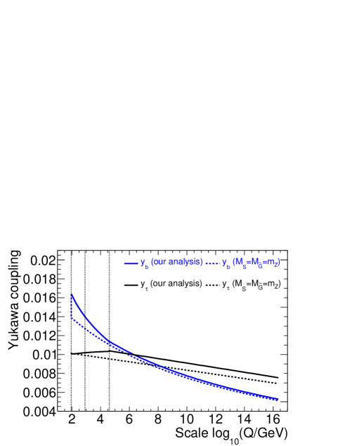
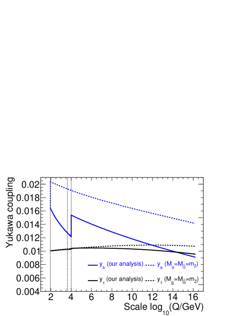
First, we show examples of the renormalization group runnings of the Yukawa coupling constants from the electroweak scale to the GUT scale. In Fig. 1, we show how the Yukawa coupling constants of $b$ and $\tau$ depend on the renormalization scale $Q$, taking $\tan\beta=3.95$, $m_{3/2}=50\ {\rm TeV}$, $m_{\bf 10}=m_{\bf\bar{5}}=m_{3/2}$, $m_{H{\bf 5}}=m_{H{\bf\bar{5}}}=0.8m_{3/2}$ and $\mu>0$ (left). If the $b$-$\tau$ unification is studied by directly matching the SM (after the electroweak symmetry breaking) to the MSSM at $Q=m_{Z}$, some of the effects of the renormalization-group runnings are not fully taken into account. In addition, with such a procedure, the effects of the wave function renormalization of the SM Higgs boson on the running of the Yukawa coupling constants of $b$ and $\tau$ may be nectlected. The renormalization group runnings of the Yukawa coupling constants with such an analysis are also shown in Fig. 1 to see the difference. We can see that the difference between the results of two analyses is sizable. With the present choice of parameters, we found that $R_{b\tau}\sim 0.7$ with our analysis which properly takes into account the mass splittings among MSSM particles, while $R_{b\tau}\sim 0.75$ with the analysis taking $M_{S}=M_{\tilde{G}}=m_{Z}$. In fact, we found that the difference becomes larger if we take larger value of $\tan\beta$. To see this, we also show the renormalization group runnings, taking $\tan\beta=40.0,\ m_{3/2}=250\ {\rm TeV}$, $m_{\bf 10}=12\ {\rm TeV}$, $m_{\bf\bar{5}}=7\ {\rm TeV}$, $m_{H{\bf 5}}=m_{H{\bf\bar{5}}}=2\ {\rm TeV}$ and $\mu>0$ (right). We can see a significant difference between the two results. This is due to the fact that, with large $\tan\beta$, the threshold correction to $y_{b}$ at $Q=M_{S}$ becomes large so that the GUT scale value of the Yukawa coupling constants becomes sensitive what kind of RGEs are used between $m_{Z}\leq Q\leq M_{S}$. The $R_{b\tau}$ parameter gives important information about the GUT scale values of the Yukawa coupling constants and the possible size of the threshold corrections to the Yukawa coupling constants at the GUT scale. Thus, an accurate calculation of $R_{b\tau}$ is important, for which, as we have seen, the use of proper effective theory at each energy scale is needed.

To see how $R_{b\tau}$ depends on various model parameters, we randomly choose $\sim 5\times 10^{4}$ sample points from the following parameter space:

• $1.1\leq\tan\beta\leq 60$,

• $40\,{\rm TeV}\leq m_{3/2}\leq 250\,{\rm TeV}$,

• $1\,{\rm TeV}\leq m_{X}\leq 100\,{\rm TeV}$ (with $X={\bf\bar{5}}$, ${H{\bf 5}}$, and ${H{\bf\bar{5}}}$),

• $\mu>0$,

and calculate $R_{b\tau}$. In the AMSB/PGM scenario, the soft SUSY breaking scalar mass squared parameters (i.e., $m_{\bf 10}^{2}$, $m_{\bf\bar{5}}^{2}$, $m_{H{\bf 5}}^{2}$, and $m_{H{\bf\bar{5}}}^{2}$ in the present set up) are expected to be of $O(m_{3/2}^{2})$. However, we also study the parameter regions where scalar masses and $m_{3/2}$ are hierarchical. As we will see in the following, the sign of the $\mu$-parameter is preferred to be positive to make $R_{b\tau}$ close to $1$. Thus, the scan is performed only in the parameter space with $\mu>0$.

Figure 2: The distribution of the sample points on $m_{\bf 10}$ vs. $\tan\beta$, $m_{\bf\bar{5}}$ vs. $\tan\beta$, $m_{3/2}$ vs. $\tan\beta$, and $m_{\tilde{B}}/m_{\tilde{W}}$ vs. $m_{\tilde{g}}/m_{\tilde{W}}$ planes. The colors of the dots indicate the smallest value of $|R_{b\tau}-1|$: $|R_{b\tau}-1|<0.1$ (red), $0.1<|R_{b\tau}-1|<0.2$ (green), and $|R_{b\tau}-1|>0.2$ (blue).

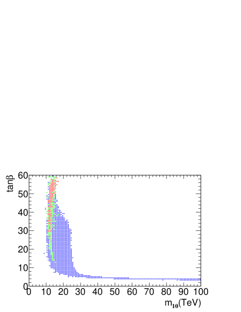
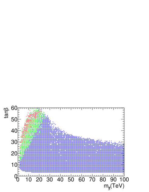
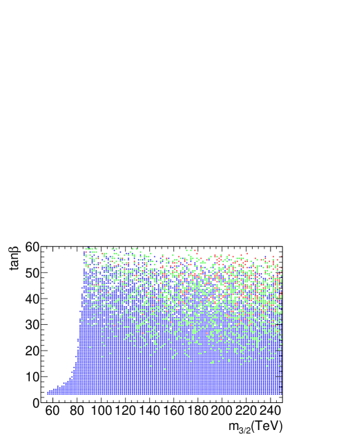
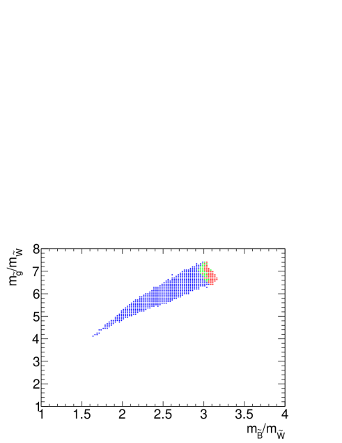
In Fig. 2, we show the distribution of the sample points we studied on $m_{\bf 10}$ vs. $\tan\beta$, $m_{\bf\bar{5}}$ vs. $\tan\beta$, $m_{3/2}$ vs. $\tan\beta$, and $m_{\tilde{B}}/m_{\tilde{W}}$ vs. $m_{\tilde{g}}/m_{\tilde{W}}$ planes (with $m_{\tilde{B}}$, $m_{\tilde{W}}$, and $m_{\tilde{g}}$ being the on-shell masses of Bino, Wino, and gluino, respectively). Here, we divide each plane into $120\times 100$ grids. Then, if at least one sample point falls into the grid, we put a dot on the grid. The colors of the dots indicate the smallest value of $|R_{b\tau}-1|$ we found: $|R_{b\tau}-1|<0.1$ (red), $0.1<|R_{b\tau}-1|<0.2$ (green), and $|R_{b\tau}-1|>0.2$ (blue). (Thus, the dots do not represent the sample points.)

From the plot on the $m_{\tilde{B}}/m_{\tilde{W}}$ vs. $m_{\tilde{g}}/m_{\tilde{W}}$ plane, we can see that the Wino becomes the lightest among the gauginos, and hence the Wino-like neutralino becomes the LSP in the parameter space we studied. We have imposed the following experimental constraints on the gaugino masses from the direct searches of gluino and long-lived Wino:

• $m_{\tilde{g}}>1.5\ {\rm TeV}$ [1, 2],

• $m_{\tilde{W}}>270\ {\rm GeV}$ [44, 45].

We show only the points consistent with the above constraints. Notice that, in the present model, all the sfermion masses are multi-TeV or larger so that the experimental bounds on them are unimportant.

From the scatter plot on the $m_{\bf 10}$ vs. $\tan\beta$ plane, one can see that $m_{\bf 10}$ and $\tan\beta$ are strongly correlated. This is because the lightest Higgs mass $m_{h}$ is mostly determined by these two parameters. In the MSSM, the lightest Higgs mass is predicted to be smaller than $m_{Z}|\cos 2\beta|$ at the tree level, and a sizable radiative correction is necessary to push the Higgs mass up to $\sim 125\ {\rm GeV}$. In general, there are two important sources of the radiative correction; one is the renormalization-group running of the quartic Higgs coupling from $M_{\rm S}$ to the weak scale, and the other is the threshold correction at $Q=M_{\rm S}$ due to stop-stop-Higgs tri-linear coupling constant. In the present model, the tri-linear coupling is one-loop suppressed so that the latter effect is insignificant. Consequently, the Higgs mass is mostly determined by the stop masses (which are determined by $m_{\bf 10}$) and $\tan\beta$; in particular, larger values of the stop masses are required to realize $m_{h}\simeq 125\ {\rm GeV}$ as $\tan\beta$ decreases. As a result, there are two regimes in the parameter space. One is with $m_{\bf 10}\lesssim 25\ {\rm TeV}$, resulting in hierarchical masses $(m_{\bf 10}/m_{3/2})^{2}\lesssim 10^{-2}$ and large $\tan\beta\gtrsim 10$; in such a region, $R_{b\tau}$ can be close to the unity. The other is with $m_{\bf 10}\gtrsim 25\ {\rm TeV}$, where $m_{\bf 10}$ can be of the same order of $m_{3/2}$ and $\tan\beta$ becomes $\sim O(1)$; in such a region, $R_{b\tau}$ is suppressed to be $\sim 0.7$.

Figure 3: The distribution of the sample points on $m_{\tilde{g}}$ vs. $R_{b\tau}$, $\tan\beta$ vs. $R_{b\tau}$, $m_{\bf 10}$ vs. $R_{b\tau}$, $m_{\bf\bar{5}}$ vs. $R_{b\tau}$, $(m_{\bf 10}/m_{3/2})^{2}$ vs. $R_{b\tau}$, and $(m_{\bf\bar{5}}/m_{3/2})^{2}$ vs. $R_{b\tau}$ planes. The colors of the dots show the largest value of $(m_{\bf 10}/m_{3/2})^{2}$: $(m_{\bf 10}/m_{3/2})^{2}>0.1$ (red), $0.01<(m_{\bf 10}/m_{3/2})^{2}<0.1$ (green), and $(m_{\bf 10}/m_{3/2})^{2}<0.01$ (blue).

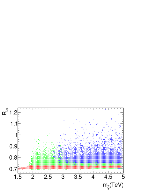
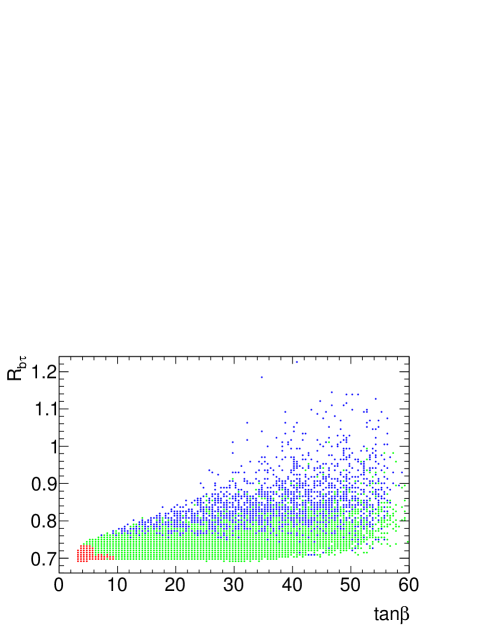
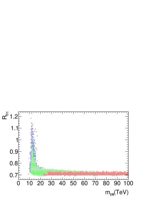
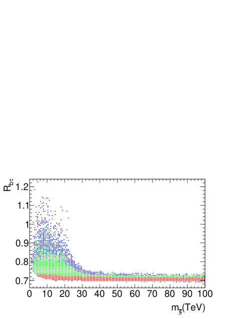
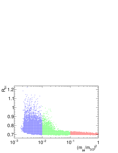
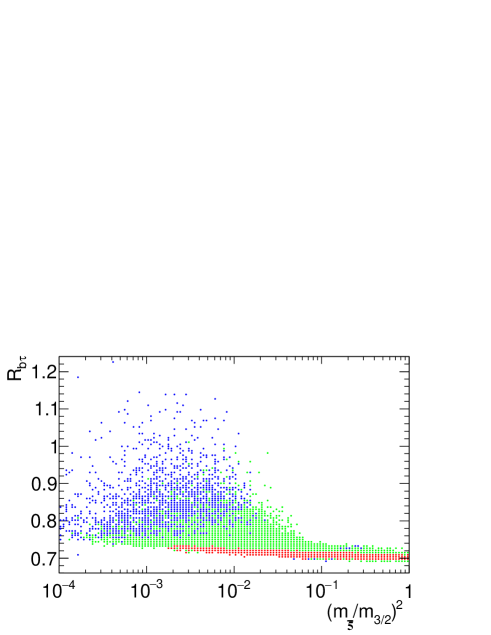
In Fig. 3, we show the result of our random scan on $m_{\tilde{g}}$ vs. $R_{b\tau}$, $\tan\beta$ vs. $R_{b\tau}$, $m_{\bf 10}$ vs. $R_{b\tau}$, $m_{\bf\bar{5}}$ vs. $R_{b\tau}$, $(m_{\bf 10}/m_{3/2})^{2}$ vs. $R_{b\tau}$, and $(m_{\bf\bar{5}}/m_{3/2})^{2}$ vs. $R_{b\tau}$ planes. As Fig. 2, we divide the planes into grids, and put a dot on the grid if there is at least one sample point falling into the grid. The colors of the dots show the largest value of $(m_{\bf 10}/m_{3/2})^{2}$ we found: $(m_{\bf 10}/m_{3/2})^{2}>0.1$ (red), $0.01<(m_{\bf 10}/m_{3/2})^{2}<0.1$ (green), and $(m_{\bf 10}/m_{3/2})^{2}<0.01$ (blue). We notice here that, on the $\tan\beta$ vs. $R_{b\tau}$ plane, the dots exist only for $\tan\beta\gtrsim 3$. This is because the scan is restricted to the parameter region of $m_{\bf 10}<100\ {\rm TeV}$, and hence the stop mass is at most $\sim 100\ {\rm TeV}$. If a larger value of $m_{\bf 10}$ is considered, smaller value of $\tan\beta$ is allowed.

From Fig. 3, it is suggested that, in order to make $R_{b\tau}$ close to $1$, (i) the scalar masses should be suppressed compared to $m_{3/2}$, (ii) $\tan\beta$ should be large, and (iii) $\mu>0$. This is because $R_{b\tau}$ becomes $\sim 0.7$ when the threshold correction $\Delta_{b}$ is negligible. In particular, we found that the renormalization-group effect between the weak scale and $M_{\rm S}$ significantly suppresses $y_{b}$, which makes $R_{b\tau}$ smaller. The conditions (i) and (ii) are necessary to enhance $\Delta_{b}$. In addition, the condition (iii) is necessary to make $\Delta_{b}$ negative. However, the condition (i) may conflict with the simple expectation from the AMSB/PGM scenario which requires the soft SUSY breaking scalar masses to be of $O(m_{3/2})$ [17]. The condition (ii), combined with $m_{h}\simeq 125\ {\rm GeV}$, suggests that $m_{\bf 10}\sim 10\ {\rm TeV}$, as can be seen in the plot on the $m_{\bf 10}$ vs. $\tan\beta$ plane of Fig. 2. From the plot on the $m_{\bf 5}$ vs. $\tan\beta$ plane, one can also see that the sample points with small $|R_{b\tau}-1|$ concentrate on the region with relatively small $m_{\bf\bar{5}}$. This is because $m_{H_{u}}^{2}(M_{\rm S})$ decreases for decreasing $m_{\bf\bar{5}}$ due to the renormalization group effect, and the small $m_{H_{u}}^{2}(M_{\rm S})$ enhances $\mu^{2}$ determined by the electroweak symmetry breaking condition. Since $\Delta_{b}$ is proportional to $\mu$, the small $m_{\bf\bar{5}}$ is favored.

Figure 4: $R_{b\tau}$ as a function of $m_{3/2}$, taking $m_{\bf\bar{5}}=m_{\bf 10}$, and $m_{H{\bf 5}}=m_{H{\bf\bar{5}}}=0.8m_{\bf 10}$ for $\mu>0$ (left), $\mu<0$ (right). The value of $\tan\beta$ is taken to be $2.4$, $3$, $4$, $6$, $10$, $20$, and $40$ as shown in the figure. The light gray (dotted) part of the lines correspond to the regions excluded by the Wino or gluino mass bounds. The marks on the lines show the points with $(m_{\bf 10}/m_{3/2})^{2}$ = 1.0($\bigstar$), 0.1($\blacktriangledown$), 0.03($\bullet$), 0.01($\blacksquare$), and 0.003($\blacktriangle$).

Figure 5: $R_{b\tau}$ as a function of $m_{3/2}$, taking $m_{\bf 10}=m_{\bf\bar{5}}=m_{3/2}$, and $m_{H{\bf 5}}=m_{H{\bf\bar{5}}}=0.8m_{3/2}$. The upper and lower lines are for $\mu>0$ and $\mu<0$, respectively. The light gray (dotted) part of the lines correspond to the regions excluded by the Wino or gluino mass bounds. The cross mark on each line shows the point with $m_{\tilde{W}}=3.0\ {\rm TeV}$. The other marks on the lines show the points with $\tan\beta$ = 4.0 ($\bigstar$), 3.5 ($\blacktriangledown$), 3.0 ($\bullet$), and 2.4($\blacksquare$).

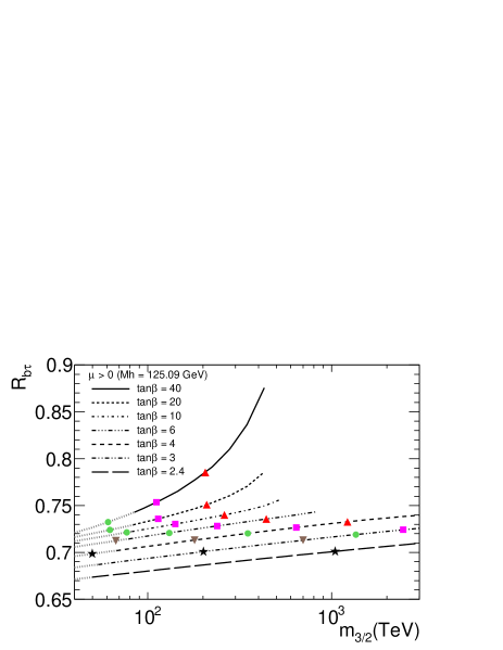
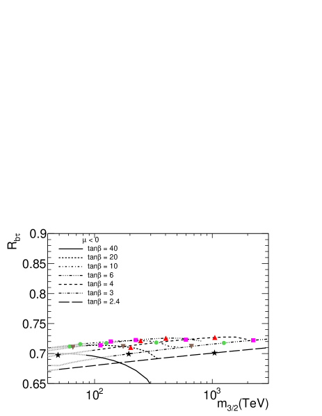
In order to see how $R_{b\tau}$ depends on the masses of SUSY particles, we calculate $R_{b\tau}$ by taking $m_{\bf\bar{5}}=m_{\bf 10}$, and $m_{H{\bf 5}}=m_{H{\bf\bar{5}}}=0.8m_{\bf 10}$. Then, with $\tan\beta$ being fixed, only one free parameter remains, which is chosen to be $m_{3/2}$. In Fig. 4, $R_{b\tau}$ is plotted as a function of $m_{3/2}$ for several values of $\tan\beta$. We also show the ratio of $m_{\bf 10}/m_{3/2}$ on each line. Some of the lines end at the middle of the figure. This is because, with $m_{\rm 10}^{2}$ being positive, the Higgs mass of $\sim 125\ {\rm GeV}$ cannot be realized if the gravitino mass is too large. For $\mu>0$, $R_{b\tau}$ becomes enhanced with larger $m_{3/2}$ or with larger $\tan\beta$; such a choice of parameters makes $\Delta_{b}$ being negative and sizable, resulting in the suppression of the bottom Yukawa coupling constant below $M_{\rm S}$. For $\mu<0$, on the contrary, $R_{b\tau}$ becomes suppressed with larger $m_{3/2}$ or larger $\tan\beta$ in the large $\tan\beta$ region ($\tan\beta\gtrsim 10$) since the sign of $\Delta_{b}$ is positive in this case. In the low $\tan\beta$ region ($\tan\beta\lesssim 10$) with $\mu<0$, this is not the case since the heavy Higgs contributions to $\Delta_{b}$, whose sign is uncorrelated to the sign of $\mu$, become comparable to the sbottom-gluino and stop-chargino contributions. We note here that, in Fig. 4, we consider the the gravitino mass up to a few PeV, with which the Wino mass becomes $\sim 3\ {\rm TeV}$. In such a parameter region, the neutral Wino is the LSP and hence the thermal relic density of the Wino becomes comparable to the dark matter density [16].

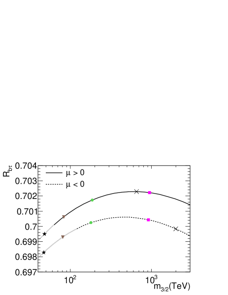
We can see that $R_{b\tau}\sim 0.7$ for both $\mu>0$ and $\mu<0$ when the scalar masses are of the same order of $m_{3/2}$. This fact indicates that, in the AMSB/PGM scenario, the threshold correction at the GUT scale needs to be sizable for successful Yukawa unification. To make this point clearer, we calculate $R_{b\tau}$ for the case where all the scalar masses are of the same order of $m_{3/2}$. In Fig. 5, we plot $R_{b\tau}$ as a function of $m_{3/2}$, taking $m_{\bf\bar{5}}=m_{\bf 10}=m_{3/2}$, and $m_{H{\bf 5}}=m_{H{\bf\bar{5}}}=0.8m_{3/2}$. In this case, masses of all the sfermions, including stops, are required to be much heavier than $\sim 10\ {\rm TeV}$, and hence relatively small $\tan\beta$ is needed. (See Fig. 2.) On each line, we show the value of $\tan\beta$. We can see that $R_{b\tau}\sim 0.7$ with such a choice of parameters; this is because $\Delta_{b}$ is suppressed due to the smallness of $\tan\beta$.

So far, we have seen that a significant hierarchy between the scalar masses and the gravitino mass is needed to make $R_{b\tau}$ close to $1$. If we require $|R_{b\tau}-1|<0.1$, for example, $m_{\bf 10}^{2}$ and $m_{\bf\bar{5}}^{2}$ are required to be of $O(1)\ \%$ of $m_{3/2}^{2}$. Because the supergravity effects are expected to make the SUSY breaking mass squared parameters to be of $O(m_{3/2}^{2})$, such a choice of $m_{\bf 10}^{2}$ and $m_{\bf\bar{5}}^{2}$ require the tuning of the parameters in the Kähler potential at the level of $O(1)\ \%$.

Figure 6: Same as Fig. 4 for $\mu>0$, except for $m_{h}=123.09\ {\rm GeV}$ (left) and $127.09\ {\rm GeV}$ (right).

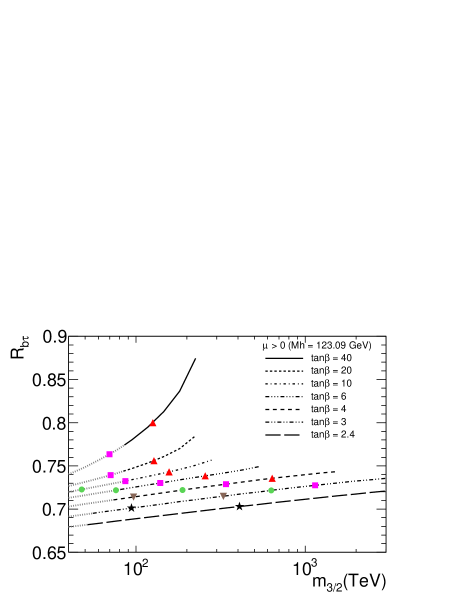
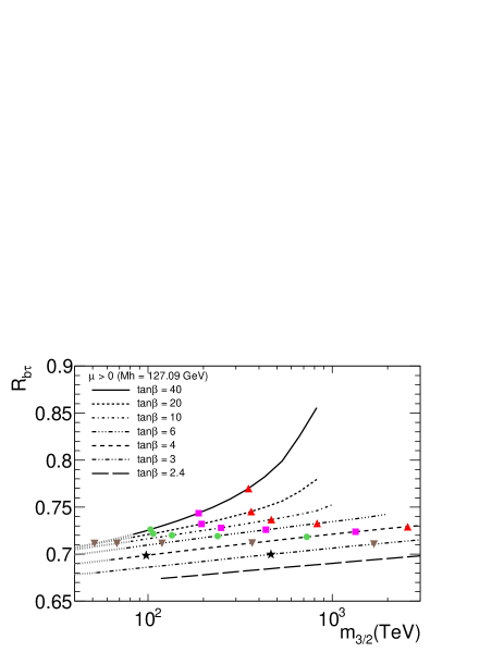
We would also like to comment on the effects of the uncertainty in the Higgs mass. Although, experimentally, the Higgs mass is determined with the accuracy of $0.21\ {\rm GeV}$, it is expected that the theoretical calculation of the Higgs mass has larger uncertainty of a few GeV. In order to see how our results change with the variation of the Higgs mass, we calculate $R_{b\tau}$ using $m_{h}=123.09\ {\rm GeV}$ and $127.09\ {\rm GeV}$, taking $m_{\bf\bar{5}}=m_{\bf 10}$, $m_{H{\bf 5}}=m_{H{\bf\bar{5}}}=0.8m_{\bf 10}$, and $\mu>0$. The results are shown in Fig. 6. Comparing with Fig. 4, we can see that, even if we vary the threoretical prediction of the Higgs mass within the theoretical uncertainty, $R_{b\tau}\sim 0.7$ when the gluino masses are much smaller than the sfermion masses. Thus, our main results are unchanged.

Before closing this section, we also study the difference between $y_{b}(M_{\rm GUT})$ and $y_{\tau}(M_{\rm GUT})$:

$$\delta y_{\bf\bar{5}}\equiv y_{b}(M_{\rm GUT})-y_{\tau}(M_{\rm GUT}).$$ (3.2)

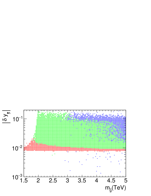
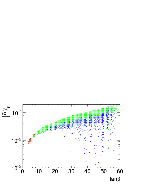
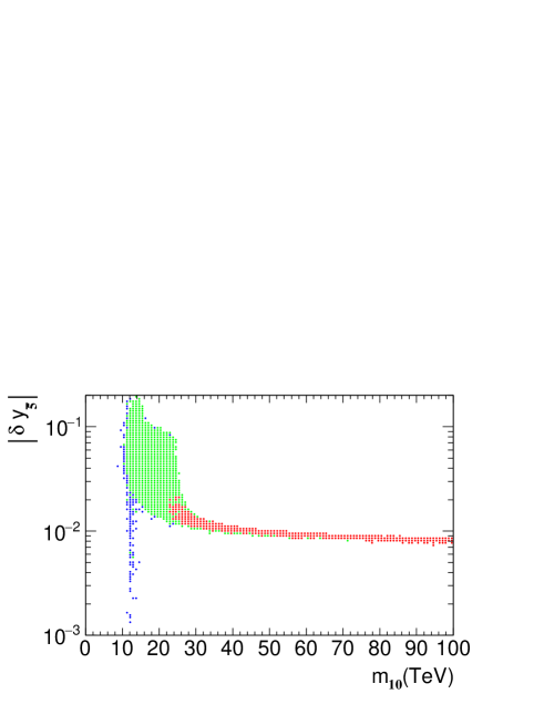
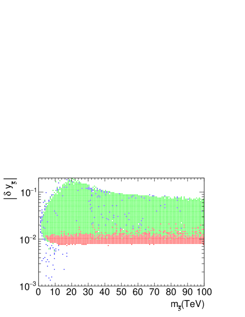
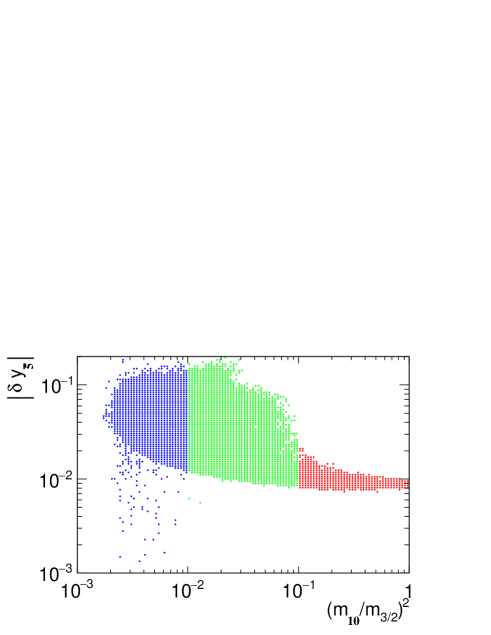
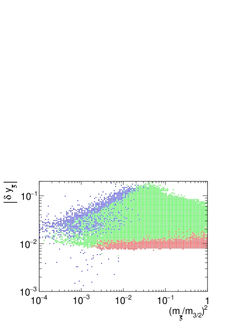
In order to see how large $\delta y_{\bf\bar{5}}$ is in the AMSB/PGM scenario, in Fig. 7, we show the distribution of $|\delta y_{\bf\bar{5}}|$ as a result of our scan. As one can see, $|\delta y_{\bf\bar{5}}|$ becomes smaller as $\tan\beta$ decreases; this is due to the smallness of $y_{b}$ and $y_{\tau}$ in the region with relatively small $\tan\beta$. Implication of this will be discussed in the next section.

Figure 7: The distribution of the sample points on $m_{\tilde{g}}$ vs. $|\delta y_{\bf\bar{5}}|$, $\tan\beta$ vs. $|\delta y_{\bf\bar{5}}|$, $m_{\bf 10}$ vs. $|\delta y_{\bf\bar{5}}|$, $m_{\bf\bar{5}}$ vs. $|\delta y_{\bf\bar{5}}|$, $(m_{\bf 10}/m_{3/2})^{2}$ vs. $|\delta y_{\bf\bar{5}}|$, and $(m_{\bf\bar{5}}/m_{3/2})^{2}$ vs. $|\delta y_{\bf\bar{5}}|$ planes. The meanings of the colors are the same as those in Fig. 3.

4 Implications

Let us now discuss implications of our numerical results. In particular, we consider how small $|R_{b\tau}-1|$ should be in order for the successful $b$-$\tau$ unification. If $y_{b}(M_{\rm GUT})\neq y_{\tau}(M_{\rm GUT})$, the difference is expected to be compensated by corrections at the GUT scale. The possible size of the corrections at the GUT scale is strongly model-dependent.

Due to the mass splitting of the particles at the GUT scale, $R_{b\tau}$ may deviate from $1$. We expect that the threshold correction due to such a mass splitting is estimated as

$$\delta y_{f}\sim\beta_{y_{f}}\log\frac{M_{\rm GUT}+\delta M_{\rm GUT}}{M_{\rm GUT}},$$ (4.1)

with $f=b$ and $\tau$, where $\beta_{y_{f}}$ denotes the $\beta$-function of $y_{f}$, and $\delta M_{\rm GUT}$ is the typical size of the mass splitting of the GUT-scale particles. As far as $\delta M_{\rm GUT}\sim O(M_{\rm GUT})$, such an effect results in $|R_{b\tau}-1|$ of $O(10^{-2})$, because $\beta_{y_{f}}$ is at most of the order of $y_{f}/16\pi^{2}$, and hence $R_{b\tau}\sim 0.7$ is hardly explained by this effect.

Another class of correction may come from the effective operators containing the fields which is responsible for the breaking of the GUT symmetry. Schematically, the superpotential responsible for such a correction, which is dimension-$5$ or higher, can be written as

$$W_{\rm Higher\,Dim.}=\frac{c}{M_{*}}\Sigma T\bar{F}\bar{H},$$ (4.2)

where $M_{*}$ is the mass scale of the mechanism generating $W_{\rm Higher\,Dim.}$, while $c$ is determined by the coupling constants in the model. Here, $\bar{F}$ and $T$ are superfield in ${\bf\bar{5}}$ and ${\bf 10}$ representations of $SU(5)$, which contain third generation quarks and leptons, and $\bar{H}$ is the superfield in ${\bf\bar{5}}$ representation containing down-type Higgs. In addition, $\Sigma$ is the field responsible for the breaking of $SU(5)\rightarrow SU(3)_{C}\times SU(2)_{L}\times U(1)_{Y}$; hereafter, to make our points clearer, $\Sigma$ is assumed to be in the adjoint representation of $SU(5)$.

The superpotential of the form of Eq. (4.2) may arise from an unknown non-perturbative dynamics at the cut-off scale (like the Planck or string scale, identifying $M_{*}$ as a cut-off scale), or by integrating out particles whose masses are above the GUT scale. Here, let consider a simple example of the latter. We introduce the following superpotential:

$$W^{\prime}=M_{*}F^{\prime}\bar{F}^{\prime}+\kappa\Sigma F^{\prime}\bar{F}+y_{\bf\bar{5}}^{\prime}T\bar{F}^{\prime}\bar{H}+y_{\bf\bar{5}}T\bar{F}\bar{H},$$ (4.3)

where $F^{\prime}$ and $\bar{F}^{\prime}$ are new superfields in ${\bf 5}$ and ${\bf\bar{5}}$ representations, respectively; with $M_{*}\gtrsim M_{\rm GUT}$, the superpotential of the form of Eq. (4.2) is obtained after integrating out $F^{\prime}$ and $\bar{F}^{\prime}$. We denote the vacuum expectation value of $\Sigma$ as $\langle\Sigma\rangle={\rm diag}(2\sigma,2\sigma,2\sigma,-3\sigma,-3\sigma)$, assuming that $\sigma\sim O(M_{\rm GUT})$. Then, with the superpotential given in Eq. (4.3), $b_{R}^{c}$ and $l_{L}$ are given by

$$b_{R}^{c} =\bar{F}_{3}\cos\theta_{b_{R}^{c}}+\bar{F}^{\prime}_{3}\sin\theta_{b_{R}^{c}},$$ (4.4)

$$l_{L} =\bar{F}_{2}\cos\theta_{l_{L}}+\bar{F}^{\prime}_{2}\sin\theta_{l_{L}},$$ (4.5)

where $\bar{F}_{3}^{(\prime)}$ and $\bar{F}_{2}^{(\prime)}$ are upper three and lower two components of $\bar{F}^{(\prime)}$, respectively, and

$$\tan\theta_{b_{R}^{c}}=-\frac{2\kappa\sigma}{M_{*}},~{}~{}~{}\tan\theta_{l_{L}}=\frac{3\kappa\sigma}{M_{*}}.$$ (4.6)

Then, the Yukawa coupling constants of $b$ and $\tau$ at the GUT scale are estimated as

$$y_{b}(M_{\rm GUT}) =y_{\bf\bar{5}}-2\epsilon y_{\bf\bar{5}}^{\prime}+O(\epsilon^{2}),$$ (4.7)

$$y_{\tau}(M_{\rm GUT}) =y_{\bf\bar{5}}+3\epsilon y_{\bf\bar{5}}^{\prime}+O(\epsilon^{2}),$$ (4.8)

with

$$\epsilon\equiv\frac{\kappa\sigma}{M_{*}},$$ (4.9)

and hence

$$R_{b\tau}=1-5\epsilon\frac{y_{\bf\bar{5}}^{\prime}}{y_{\bf\bar{5}}}+O(\epsilon^{2}).$$ (4.10)

In addition,

$$\delta y_{\bf\bar{5}}\simeq-5\epsilon y_{\bf\bar{5}}^{\prime}+O(\epsilon^{2}).$$ (4.11)

$R_{b\tau}$ may significantly deviate from $1$ in this set up. If $y_{\bf\bar{5}}^{\prime}\sim y_{\bf\bar{5}}$, $|R_{b\tau}-1|\sim O(0.1)$ requires $\epsilon\sim O(0.1)$. In such a case, the quarks and leptons, which are embedded into the same $SU(5)$ multiplet in the simplest scenario, are given by different admixture of the fields at the GUT scale or above. On the contrary, for $y_{\bf\bar{5}}^{\prime}\gg y_{\bf\bar{5}}$, $|R_{b\tau}-1|\sim O(0.1)$ is possible even with $\epsilon\ll O(0.1)$. In particular, when $\tan\beta$ is not so large, $y_{b}$ and $y_{\tau}$ are much smaller than $1$ and hence $\delta y_{\bf\bar{5}}\ll 1$ (see Fig. 7). Then, the $b$-$\tau$ unification may be realized with $M_{*}$ much larger than the GUT scale (like $M_{*}$ as large as the Planck scale). In such a case, however, the quarks and leptons have new Yukawa interactions much stronger than those in the MSSM, which may introduce new flavor and CP problems in SUSY model. In particular, it is unclear if the new field $F^{\prime}$ selectively couples to the third generation quarks and leptons. If the coupling between $F^{\prime}$ and first or second generation quarks and leptons is as strong as that to third generation ones, the hierarchy of the SM Yukawa coupling constants are easily spoiled. We also note here that, if non-trivial flavor mixings or CP violations exist in such new couplings, they may affect the SUSY breaking scalar mass squared parameters via the renormalization group runnings [46]. Such an effect may give sizable contributions to low energy flavor and CP violating observables.

5 Summary

We have studied the $b$-$\tau$ unification in SUSY model with the AMSB/PGM mass spectrum. In the model of our interest, sfermions as well as Higgsinos acquire masses from direct interactions with SUSY breaking fields while gaugino masses are from AMSB effect. Consequently, the gaugino masses (as well as the SUSY breaking tri-linear scalar coupling constants) are one-loop suppressed compared to the sfermion masses. In order for the accurate study of the renormalization group effects on coupling constants, we have considered three different effective theories, i.e., SM, $\tilde{G}$SM, and MSSM. We have used a numerical program in which the two-loop RGEs in these effective theories, as well as threshold corrections at the matching scales, are implemented, and calculated the Yukawa coupling constants at the GUT scale. In order to understand the viability of the Yukawa unification in the AMSB/PGM scenario, we have performed the parameter scan and calculated $y_{b}(M_{\rm GUT})$ and $y_{\tau}(M_{\rm GUT})$ for about $5\times 10^{4}$ sample points.

We have found that the naive mass spectrum of the AMSB/PGM scenario, in which the sfermion masses are of the order of the gravitino mass, predicts $y_{b}(M_{\rm GUT})\sim 0.7y_{\tau}(M_{\rm GUT})$, which conflicts with the $b$-$\tau$ Yukawa unification in the simple set up. In order to solve this discrepancy, one may consider sizable corrections at the GUT scale. In such a case, a non-trivial flavor structure is suggested at the GUT scale, which may affect low-energy flavor and CP violating observables. Another resolution may be to adopt suppressed sfermion masses compared to the gravitino mass. As a result of our parameter scan, we found sample points with $|R_{b\tau}-1|<0.1$, for example, when the sfermion mass squared parameters, $m_{\bf 10}^{2}$ and $m_{\bf\bar{5}}^{2}$, are of $O(1)\ \%$ of $m_{3/2}^{2}$. Because the expectation is that $m_{\bf 10}^{2}$ and $m_{\bf\bar{5}}^{2}$ are of $O(m_{3/2}^{2})$, this may suggest the $O(1)\ \%$ level tuning of the parameters in the Kähler potential to suppress the scalar masses.

Acknowledgements: The work of T.M. is supported by JSPS KAKENHI No. 26400239.

References

- [1] The ATLAS collaboration, ATLAS-CONF-2015-062.
- [2] V. Khachatryan et al. [CMS Collaboration], [arXiv:1602.06581 [hep-ex]].
- [3] Y. Okada, M. Yamaguchi and T. Yanagida, Prog. Theor. Phys. 85 (1991) 1.
- [4] Y. Okada, M. Yamaguchi and T. Yanagida, Phys. Lett. B 262, 54 (1991).
- [5] J. R. Ellis, G. Ridolfi and F. Zwirner, Phys. Lett. B 257 (1991) 83.
- [6] J. R. Ellis, G. Ridolfi and F. Zwirner, Phys. Lett. B 262, 477 (1991).
- [7] H. E. Haber and R. Hempfling, Phys. Rev. Lett. 66 (1991) 1815.
- [8] K. A. Olive et al. [Particle Data Group Collaboration], Chin. Phys. C 38 (2014) 090001.
- [9] E. Bagnaschi, G. F. Giudice, P. Slavich and A. Strumia, JHEP 1409 (2014) 092 [arXiv:1407.4081 [hep-ph]].
- [10] G. F. Giudice, M. A. Luty, H. Murayama and R. Rattazzi, JHEP 9812 (1998) 027 [hep-ph/9810442].
- [11] L. Randall and R. Sundrum, Nucl. Phys. B 557 (1999) 79 [hep-th/9810155].
- [12] M. Ibe, T. Moroi and T. T. Yanagida, Phys. Lett. B 644 (2007) 355 [hep-ph/0610277].
- [13] M. Ibe and T. T. Yanagida, Phys. Lett. B 709 (2012) 374 [arXiv:1112.2462 [hep-ph]].
- [14] N. Arkani-Hamed, A. Gupta, D. E. Kaplan, N. Weiner and T. Zorawski, arXiv:1212.6971 [hep-ph].
- [15] T. Moroi and L. Randall, Nucl. Phys. B 570 (2000) 455 [hep-ph/9906527].
- [16] J. Hisano, S. Matsumoto, M. Nagai, O. Saito and M. Senami, Phys. Lett. B 646 (2007) 34 [hep-ph/0610249].
- [17] K. Tobe and J. D. Wells, Nucl. Phys. B 663 (2003) 123 [hep-ph/0301015].
- [18] G. Ross and M. Serna, Phys. Lett. B 664 (2008) 97 [arXiv:0704.1248 [hep-ph]].
- [19] S. Antusch and M. Spinrath, Phys. Rev. D 78 (2008) 075020 [arXiv:0804.0717 [hep-ph]].
- [20] S. Antusch and M. Spinrath, Phys. Rev. D 79 (2009) 095004 [arXiv:0902.4644 [hep-ph]].
- [21] H. Baer, I. Gogoladze, A. Mustafayev, S. Raza and Q. Shafi, JHEP 1203 (2012) 047 [arXiv:1201.4412 [hep-ph]].
- [22] H. Baer, S. Raza and Q. Shafi, Phys. Lett. B 712 (2012) 250 [arXiv:1201.5668 [hep-ph]].
- [23] M. Badziak, Mod. Phys. Lett. A 27 (2012) 1230020 [arXiv:1205.6232 [hep-ph]].
- [24] A. S. Joshipura and K. M. Patel, Phys. Rev. D 86 (2012) 035019 [arXiv:1206.3910 [hep-ph]].
- [25] G. Elor, L. J. Hall, D. Pinner and J. T. Ruderman, JHEP 1210 (2012) 111 [arXiv:1206.5301 [hep-ph]].
- [26] H. Baer, S. Kraml and S. Kulkarni, JHEP 1212 (2012) 066 [arXiv:1208.3039 [hep-ph]].
- [27] A. Anandakrishnan, S. Raby and A. Wingerter, Phys. Rev. D 87 (2013) 055005 [arXiv:1212.0542 [hep-ph]].
- [28] M. A. Ajaib, I. Gogoladze, Q. Shafi and C. S. Un, JHEP 1405 (2014) 079 [arXiv:1402.4918 [hep-ph]].
- [29] D. J. Miller and A. P. Morais, JHEP 1412 (2014) 132 [arXiv:1408.3013 [hep-ph]].
- [30] I. Gogoladze, A. Mustafayev, Q. Shafi and C. S. Un, Phys. Rev. D 91 (2015) 096005 [arXiv:1501.07290 [hep-ph]].
- [31] L. J. Hall, R. Rattazzi and U. Sarid, Phys. Rev. D 50 (1994) 7048 [hep-ph/9306309, hep-ph/9306309].
- [32] M. Carena, M. Olechowski, S. Pokorski and C. E. M. Wagner, Nucl. Phys. B 426 (1994) 269 [hep-ph/9402253].
- [33] T. Blazek, S. Raby and S. Pokorski, Phys. Rev. D 52 (1995) 4151 [hep-ph/9504364].
- [34] B. C. Allanach, Comput. Phys. Commun. 143 (2002) 305 [hep-ph/0104145].
- [35] D. Buttazzo, G. Degrassi, P. P. Giardino, G. F. Giudice, F. Sala, A. Salvio and A. Strumia, JHEP 1312 (2013) 089 [arXiv:1307.3536 [hep-ph]].
- [36] M. Kawasaki, K. Kohri, T. Moroi and Y. Takaesu, Phys. Lett. B 751 (2015) 246 [arXiv:1509.03665 [hep-ph]].
- [37] B. Bhattacherjee, M. Ibe, K. Ichikawa, S. Matsumoto and K. Nishiyama, JHEP 1407 (2014) 080 [arXiv:1405.4914 [hep-ph]].
- [38] G. Giesen, M. Boudaud, Y. Genolini, V. Poulin, M. Cirelli, P. Salati and P. D. Serpico, JCAP 1509 (2015) 023 [arXiv:1504.04276 [astro-ph.HE]].
- [39] H. B. Jin, Y. L. Wu and Y. F. Zhou, Phys. Rev. D 92 (2015) 055027 [arXiv:1504.04604 [hep-ph]].
- [40] C. Evoli, D. Gaggero and D. Grasso, JCAP 1512 (2015) 039 [arXiv:1504.05175 [astro-ph.HE]].
- [41] M. Ibe, S. Matsumoto, S. Shirai and T. T. Yanagida, Phys. Rev. D 91 (2015) 111701 [arXiv:1504.05554 [hep-ph]].
- [42] K. Hamaguchi, T. Moroi and K. Nakayama, Phys. Lett. B 747 (2015) 523 [arXiv:1504.05937 [hep-ph]].
- [43] S. J. Lin, X. J. Bi, P. F. Yin and Z. H. Yu, arXiv:1504.07230 [hep-ph].
- [44] G. Aad et al. [ATLAS Collaboration], Phys. Rev. D 88 (2013) 112006 [arXiv:1310.3675 [hep-ex]].
- [45] V. Khachatryan et al. [CMS Collaboration], JHEP 1501 (2015) 096 [arXiv:1411.6006 [hep-ex]].
- [46] L. J. Hall, V. A. Kostelecky and S. Raby, Nucl. Phys. B 267 (1986) 415.