Law of large numbers for the largest component in a hyperbolic model of complex networks

Abstract

We consider the component structure of a recent model of random graphs on the hyperbolic plane that was introduced by Krioukov et al. The model exhibits a power law degree sequence, small distances and clustering, features that are associated with so-called complex networks. The model is controlled by two parameters $\alpha$ and $\nu$ where, roughly speaking, $\alpha$ controls the exponent of the power law and $\nu$ controls the average degree. Refining earlier results, we are able to show a law of large numbers for the largest component. That is, we show that the fraction of points in the largest component tends in probability to a constant $c$ that depends only on $\alpha,\nu$, while all other components are sublinear. We also study how $c$ depends on $\alpha,\nu$. To deduce our results, we introduce a local approximation of the random graph by a continuum percolation model on $\mathbb{R}^{2}$ that may be of independent interest.

keywords: random graphs, hyperbolic plane, giant component, law of large numbers

2010 AMS Subj. Class.: 05C80, 05C82; 60D05, 82B43

1 Introduction

The component structure of random graphs and in particular the size of the largest component has been a central problem in the theory of random graphs as well as in percolation theory. Already from the founding paper of random graph theory [15] the emergence of the giant component is a central theme that recurs, through the development of more and more sophisticated results.

In this paper, we consider a random graph model that was introduced recently by Krioukov et al. in [23]. The aim of that work was the development of a geometric framework for the analysis of properties of the so-called complex networks. This term describes a diverse class of networks that emerge in a range of human activities or biological processes and includes social networks, scientific collaborator networks as well as computer networks, such as the Internet, and the power grid – see for example [2]. These are networks that consist of a very large number of heterogeneous nodes (nowadays social networks such as the Facebook or the Twitter have billions of users), and they are sparse. However, locally they are dense - this is the clustering phenomenon which makes it more likely for two vertices that have a common neighbour to be connected. Furthermore, these networks are small worlds: almost all pairs of vertices that are in the same component are within a short distance from each other. But probably the most strikingly ubiquitous property they have is that their degree distribution is scale free. This means that its tail follows a power law, usually with exponent between 2 and 3 (see for example [2]). Further discussion on these characteristics can be found in the books of Chung and Lu [13] and of Dorogovtsev [14].

In the past decade, several models have appeared in the literature aiming at capturing these features. Among the first was the preferential attachment model. This term describes a class of models of randomly growing graphs whose aim is to capture the following phenomenon: nodes which are already popular retain their popularity or tend to become more popular as the network grows. It was introduced by Barabási and Albert [2] and subsequently defined and studied rigorously by Bollobás, Riordan and co-authors (see for example [9], [8]).

Another extensively studied model was defined by Chung and Lu [11], [12]. In some sense, this is a generalisation of the standard binomial model $G(n,p)$. Each vertex is equipped with a weight, which effectively corresponds to its expected degree, and every two vertices are joined independently of every other pair with probability that is proportional to the product of their weights. If the distribution of these weights follows a power law, then it turns out that the degree distribution of the resulting random graph follows a power law as well. This model is a special case of an inhomogeneous random graph of rank 1 [7].

All these models have their shortcomings and none of them incorporates all the above features. For example, the Chung–Lu model exhibits a power law degree distribution (provided the weights of the vertices are suitably chosen) and average distance of order $O(\log\log N)$ (when the exponent of the power law is between 2 and 3, see [11]), but it is locally tree like (around most vertices) and therefore it does not exhibit clustering. This is also the situation in the Barabási-Albert model.

For the the Chung-Lu model, this is the case as the pairs of vertices form edges independently. But for clustering to appear, it has to be the case that for two edges that share an endvertex the probability that their other two endvertices are joined must be higher compared to that where we assume nothing about these edges. This property is naturally present in random graphs that are created over metric spaces, such as random geometric graphs. In a random geometric graph, the vertices are a random set of points on a given metric space, with any two of them being adjacent if their distance is smaller than some threshold.

The model of Krioukov et al. [23] does exactly this. It introduces a geometric framework on the theory of complex networks and it is based on the hypothesis that hyperbolic geometry underlies these networks. In fact, it turns out that the power-law degree distribution emerges naturally from the underlying hyperbolic geometry. They defined an associated random graph model, which we will describe in detail in the next section, and considered some of its typical properties. More specifically, they observed a power-law degree sequence as well as clustering properties. These characteristics were later verified rigorously by Gugelmann et al. [18] as well as by the second author [16] and Candellero and the second author [10] (these two papers are on a different, but closely related model).

The aim of the present work is the study the component structure of such a random graph. More specifically, we consider the number of vertices that are contained in a largest component of the graph. In previous work [4] with M. Bode, we have determined the range of the parameters, in which the so-called giant component emerges. We have shown that in this model this range essentially coincides with the range in which the exponent of the power law is smaller than 3. What is more, when the exponent of the power law is larger than 3, the random graph typically consists of many relatively small components, no matter how large the average degree of the graph is. This is in sharp contrast with the classical Erdős-Rényi model (see [6] or [19]) as well as with the situation of random geometric graphs on Euclidean spaces (see [26]) where the dependence on the average degree is crucial.

In the present paper, we give a complete description of this range and, furthermore, we show that the order of the largest connected component follows a law of large numbers. Our proof is based on the local approximation of the random graph model by an infinite continuum percolation model on $\mathbb{R}^{2}$, which may be of independent interest. We show that percolation in this model coincides with the existence of a giant component in the model of Krioukov et al. We now proceed with the definition of the model.

1.1 The Krioukov-Papadopoulos-Kitsak-Vahdat-Boguñá model

Let us recall very briefly some facts about the hyperbolic plane $\mathbb{H}$. The hyperbolic plane is an unbounded 2-dimensional manifold of constant negative curvature $-1$. There are several representations of it, such as the upper half-plane model, the Beltrami-Klein disk model and the Poincaré disk model. The Poincaré disk model is defined if we equip the unit disk ${\mathbb{D}}:=\{(x,y)\in\mathbb{R}^{2}\ :x^{2}+y^{2}<1\}$ with the metric given by the differential form ${\operatorname{d}}s^{2}=4~{}\frac{dx^{2}+dy^{2}}{(1-x^{2}-y^{2})^{2}}$. For an introduction to hyperbolic geometry and the properties of the hyperbolic plane, the reader may refer to the book of Stillwell [27].

A very important property that differentiates the hyperbolic plane from the euclidean is the rate of growth of volumes. In $\mathbb{H}$, a disk of radius $r$ (i.e., the set of points at hyperbolic distance at most $r$ to a given point) has area equal to $2\pi(\cosh(r)-1)$ and length of circumference equal to $2\pi\sinh(r)$. Another basic geometric fact that we will use later in our proofs is the so-called hyperbolic cosine rule. This states that if $A,B,C$ are distinct points on the hyperbolic plane, and we denote by $a$ the distance between $B,C$, by $b$ the distance between $A,C$, by $c$ the distance between $A,B$ and by $\gamma$ the angle (at $C$) between the shortest $AC$- and $BC$-paths, then it holds that $\cosh(c)=\cosh(a)\cosh(b)-\cos(\gamma)\sinh(a)\sinh(b)$.

We can now introduce the model we will be considering in this paper. We call it the Krioukov-Papadopoulos-Kitsak-Vahdat-Boguñá-model, after its inventors, but for convenience we will abbreviate this to KPKVB-model. The model has three parameters: the number of vertices $N$, which we think of as the parameter that tends to infinity, and $\alpha,\nu>0$ which are fixed (that is, do not depend on $N$). Given $N,\nu,\alpha$, we set $R:=2\log(N/\nu)$. Consider the Poincaré disk representation and let $O$ be the origin of the disk. We select $N$ points independently at random from the disk of (hyperbolic) radius $R$ centred at $O$, which we denote by ${\mathcal{D}}_{R}$, according to the following probability distribution. If the random point $u$ has polar coordinates $(r,\theta)$, then $\theta,r$ are independent, $\theta$ is uniformly distributed in $(0,2\pi]$ and the cumulative distribution function of $r$ is given by:

$$F_{\alpha,R}(r)=\left\{\begin{array}[]{cl}0&\text{ if $r<0$, }\\ \frac{\cosh(\alpha r)-1}{\cosh(\alpha R)-1}&\text{ if }0\leq r\leq R,\\ 1&\text{ if $r>R$ }\end{array}\right.$$ (1)

Note that when $\alpha=1$, then this is simply the uniform distribution on ${\mathcal{D}}_{R}$. We label the random points as $1,\ldots,N$.

It can be seen that the above probability distribution corresponds precisely to the polar coordinates of a point taken uniformly at random from the disk of radius $R$ around the origin in the hyperbolic plane of curvature $-\alpha^{2}$. Indeed, a simple calculation shows that the area of disc of radius $r$ on the hyperbolic plane of curvature $-\alpha^{2}$ is equal to $\cosh(\alpha r)-1$. So the above distribution can be viewed as selecting the $N$ points uniformly on a disc of radius $R$ on the hyperbolic plane of curvature $-\alpha^{2}$ and then projecting them onto the hyperbolic plane of curvature -1, preserving polar coordinates. This is where we create the random graph. The set of the $N$ labeled points will be the vertex set of our random graph and we denote it by $\mathrm{V}$. The KPKVB-random graph, denoted $G(N;\alpha,\nu)$, is formed when we join each pair of vertices, if and only if they are within (hyperbolic) distance $R$. Note this is precisely the radius of the disk ${\mathcal{D}}_{R}$ that the points live on. Figures 1,2 show examples of such a random graph on $N=500$ vertices.

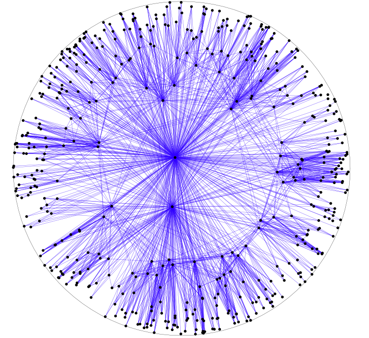
Figure 1: The random graph $G(N;\alpha,\nu)$ with $N=500$ vertices, $\nu=2$ and $\alpha=0.7$ and $3/2$.

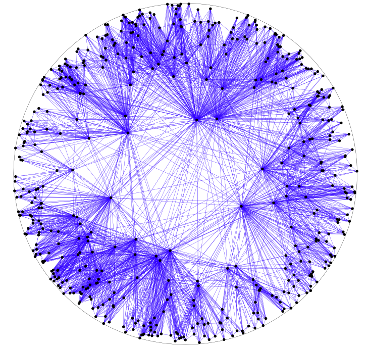
Figure 2: The random graph $G(N;\alpha,\nu)$ with $N=500$ vertices, $\alpha=1$ and $\nu=0.2$ and $10$.

Krioukov et al. [23] in fact defined a generalisation of this model where the probability distribution over the graphs on a given point set $\mathrm{V}$ of size $N$ is a Gibbs distribution which involves a temperature parameter. The model we consider in this paper corresponds to the limiting case where the temperature tends to 0.

Let us remark that the edge-set of $G(N;\alpha,\nu)$ is decreasing in $\alpha$ and increasing in $\nu$ in the following sense. We remind the reader that a coupling of two random objects $X,Y$ is a common probability space for a pair of objects $(X^{\prime},Y^{\prime})$ whose marginal distributions satisfy $X^{\prime}\hskip 0.86108pt\raisebox{-0.43057pt}{$=$}\raisebox{4.30554pt}{{$\scriptstyle d$}}\hskip 3.44444ptX,Y^{\prime}\hskip 0.86108pt\raisebox{-0.43057pt}{$=$}\raisebox{4.30554pt}{{$\scriptstyle d$}}\hskip 3.44444ptY$.

Lemma 1 ([4])

Let $\alpha,\alpha^{\prime},\nu,\nu^{\prime}>0$ be such that $\alpha\geq\alpha^{\prime}$ and $\nu\leq\nu^{\prime}$. For every $N\in\mathbb{N}$, there exists a coupling such that $G(N;\alpha,\nu)$ is a subgraph of $G(N;\alpha^{\prime},\nu^{\prime})$.

The proof can be found in our earlier paper [4] that was joint with Bode.

We should also mention that Krioukov et al. in fact had an additional parameter in their definition of the model. However, it turns out that this parameter is not necessary in the following sense. Every probability distribution (on labelled graphs) that is defined by some choice of parameters in the model with one extra parameter coincides with the probability distribution $G(N;\alpha,\nu)$ for some $N,\alpha,\nu$. This is Lemma 1.1 in [4].

Krioukov et al. [23] focus on the degree distribution of $G(N;\alpha,\nu)$, showing that when $\alpha>{1\over 2}$ this follows a power law with exponent $2\alpha+1$. They also discuss clustering on the generalised version we briefly described above. Their results on the degree distribution have been verified rigorously by Gugelmann et al. [18].

Note that when $\alpha=1$, that is, when the $N$ vertices are uniformly distributed in ${\mathcal{D}}_{R}$, the exponent of the power law is equal to 3. When ${1\over 2}<\alpha<1$, the exponent is between 2 and 3, as is the case in a number of networks that emerge in applications such as computer networks, social networks and biological networks (see for example [2]). When $\alpha={1\over 2}$ then the exponent becomes equal to 2. This case has recently emerged in theoretical cosmology [22]. In a quantum-gravitational setting, networks between space-time events are considered where two events are connected (in a graph-theoretic sense) if they are causally connected, that is, one is located in the light cone of the other. The analysis of Krioukov et al. [22] indicates that the tail of the degree distribution follows a power law with exponent 2.

As observed by Krioukov et al. [23] and rigorously proved by Gugelmann et al. [18], the average degree of the random graph can be “tuned” through the parameter $\nu$ : for $\alpha>\frac{1}{2}$, the average degree tends to $2\alpha^{2}\nu/\pi(\alpha-\frac{1}{2})^{2}$ in probability.

In [4], together with M. Bode we have showed that $\alpha=1$ is the critical point for the emergence of a “giant” component in $G(N;\alpha,\nu)$. More specifically, we have showed that when $\alpha<1$, the largest component contains a positive fraction of the vertices asymptotically with high probability, whereas if $\alpha>1$, then the largest component is sublinear. For $\alpha=1$, then the component structure depends on $\nu$. We show that if $\nu$ is large enough, then a “giant” component exists with high probability, whereas if $\nu$ is small enough, then with high probability all components have sublinear size.

Kiwi and Mitsche [21] showed that when $\alpha<1$ then the second largest component is sublinear with high probability.

In [5], together with M. Bode we studied the probability of being connected. We showed that when $\alpha<\frac{1}{2}$, then $G(N;\alpha,\nu)$ is connected with high probability, while if $\alpha>\frac{1}{2}$ the graph is disconnected with high probability. For $\alpha=\frac{1}{2}$, the probability of connectivity tends to a constant $c=c(\nu)$ that depends on $\nu$. Curiously, $c(\nu)$ equals one for $\nu\geq\pi$ while it increases strictly from zero to one as $\nu$ varies from $0$ to $\pi$.

1.2 Results

The results of this paper elaborate on the component structure of the KPKVB model, refining our previous results [4] with Bode. We show that the size of the largest component rescaled by $N$ (that is, the fraction of the vertices that belong to the largest component) converges in probability to a non-negative constant. We further determine this constant as the integral of a function that is associated with a percolation model on $\mathbb{R}^{2}$. We also show that the number of points in the second largest connected component is sublinear. When $\alpha=1$, we show that there exists a critical $\nu$ around which the constant changes from 0 to being positive. In other words, there is a critical value for $\nu$ around which the emergence of the giant component occurs. We let ${\mathscr{C}}_{(1)}$ and ${\mathscr{C}}_{(2)}$ denote the largest and second largest connected component (if the two have the same number of vertices, then the ordering is lexicographic using a labelling of the vertex set).

Theorem 2

For every $\nu,\alpha>0$ there exists a $c=c(\alpha,\nu)$ such that

$$\frac{|{\mathscr{C}}_{(1)}|}{N}\to c\quad\quad\text{ and }\quad\quad\quad\frac{|{\mathscr{C}}_{(2)}|}{N}\to 0\quad\quad\text{ in probability, }$$

as $N\to\infty$. The function $c(\alpha,\nu)$ has the following properties:

1. If $\alpha>1$ and $\nu$ arbitrary then $c=0$;

2. If $\alpha<1$ and $\nu$ arbitrary then $c>0$;

3. There exists a critical value $0<\nu_{\text{crit}}<\infty$ such that if $\alpha=1$ then

   1. if $\nu<\nu_{\text{crit}}$ then $c=0$;

   2. if $\nu>\nu_{\text{crit}}$ then $c>0$.

4. $c=1$ if and only if $\alpha\leq\frac{1}{2}$.

5. $c$ is continuous on $(0,\infty)^{2}\setminus\{1\}\times[\nu_{\text{crit}},\infty)$, and every point of $\{1\}\times(\nu_{\text{crit}},\infty)$ is a point of discontinuity.

6. $c$ is strictly decreasing in $\alpha$ on $(\frac{1}{2},1)\times(0,\infty)$ and strictly increasing in $\nu$ on $(\frac{1}{2},1)\times(0,\infty)\cup\{1\}\times(\nu_{\text{crit}},\infty)$.

The above theorem leaves open the case where $\alpha=1$ and $\nu=\nu_{\text{crit}}$. We do not know whether $c(1,\nu_{\text{crit}})$ is positive or 0. The latter would imply that $c(1,\nu)$ is continuous as a function of $\nu$. We however conjecture that $c(1,\nu_{\text{crit}})>0$.

Notation

For a sequence of real-valued random variables $X_{n}$ defined on a sequence of probability spaces, we write $X_{n}\stackrel{{\scriptstyle p}}{{\to}}a$, where $a\in\mathbb{R}$, to denote that the sequence $X_{n}$ converges to $a$ in probability. For a sequence of positive real numbers $a_{n}$, we write $X_{n}=o_{p}(a_{n})$, if $|X_{n}|/a_{n}\stackrel{{\scriptstyle p}}{{\to}}0$, as $n\to\infty$.

An event occurs almost surely (a.s.) if its probability is equal to 1. For a sequence of probability spaces $(\Omega_{n},\mathbb{P}_{n},\mathcal{F}_{n})$, we say that a sequence of measurable sets $\mathcal{E}_{n}\in\mathcal{F}_{n}$ occurs asymptotically almost surely (a.a.s.), if $\lim_{n\to\infty}\mathbb{P}_{n}(\mathcal{E}_{n})=1$.

1.2.1 Tools and outline

Roughly speaking, one can show that two vertices of radii $r_{1}$ and $r_{2}$, respectively, which are close to the periphery of ${\mathcal{D}}_{R}$ are adjacent if their relative angle is at most $e^{(y_{1}+y_{2})/2}/N$, where $y_{1}=R-r_{1}$ and $y_{2}=R-r_{2}$. Hence, conditional on $r_{1}$ and $r_{2}$, the probability that these two vertices are adjacent is proportional to $e^{(y_{1}+y_{2})/2}/N$.

We will map ${\mathcal{D}}_{R}$ onto $\mathbb{R}^{2}$ preserving $y$ and projecting the angle onto the $x$-axis scaling it by $N$. Hence, relative angle $e^{(y_{1}+y_{2})/2}/N$ between two vertices in ${\mathcal{D}}_{R}$ will project to two points in $\mathbb{R}^{2}$ whose $x$-coordinates differ by at most $e^{(y_{1}+y_{2})/2}$.

This gives rise to a continuum percolation model on $\mathbb{R}^{2}$, whose vertices are the points of an inhomogeneous Poisson point process and any two of them are joined if their positions satisfy the above condition. This continuum percolation model is a good approximation of $G(N;\alpha,\nu)$ close to the periphery of ${\mathcal{D}}_{R}$. As we shall see later in Section 4, we can couple the two using the aforementioned mapping so that the two graphs coincide close to the $x$-axis.

In Section 2, we determine the critical conditions for the parameters of the continuum percolation model that ensure the almost sure existence of an infinite component. Thereafter, in Section 4, we show how does this infinite model approximate $G(N;\alpha,\nu)$ and deduce the law of large numbers for the size of its largest and the second largest connected component. The fraction of vertices that are contained in the largest component converges in probability to a constant $c(\alpha,\nu)$. More specifically, we show that the function $c(\alpha,\nu)$ is given as the integral of the probability that a given point “percolates”, that is, it belongs to an infinite component, in the infinite model.

2 A continuum percolation model

Given a countable set of points $P=\{p_{1},p_{2},\dots\}\subset\mathbb{R}\times[0,\infty)$ in the upper half of the (euclidean) plane, we define a graph $\Gamma(P)$ with vertex set $P$ by setting

$$p_{i}p_{j}\in E(\Gamma(P))\text{ if and only if }|x_{i}-x_{j}|<e^{\frac{1}{2}(y_{i}+y_{j})}=:t(y_{i},y_{j}),$$

where we write $p_{i}=(x_{i},y_{i})$. For a point $p=(x,y)$, we let ${\mathcal{B}}(p)$ denote the ball around $p$, that is, the set $\{p^{\prime}=(x^{\prime},y^{\prime})\ :\ y^{\prime}>0,\ |x-x^{\prime}|<t(y,y^{\prime})\}$. Thus, ${\mathcal{B}}(p)$ contains all those points that would potentially connect to $p$. During our proofs, we will need the notion of the half-ball around $p$. More specifically, we denote by ${\mathcal{B}}^{+}(p)$ the set $\{p^{\prime}=(x^{\prime},y^{\prime})\ :\ y^{\prime}>0,\ 0<x^{\prime}-x<t(y,y^{\prime})\}$ and by ${\mathcal{B}}^{-}(p)$ the set $\{p^{\prime}=(x^{\prime},y^{\prime})\ :\ y^{\prime}>0,\ 0<x-x^{\prime}<t(y,y^{\prime})\}$. In other words, the ${\mathcal{B}}^{+}(p)$ consists of those points in ${\mathcal{B}}(p)$ that are located on the right of $p$ (i.e., they have larger $x$-coordinate) and ${\mathcal{B}}^{-}(p)$ consists of those points that are on the left of $p$. Finally, for a point $p\in\mathbb{R}^{2}$, we let $x(p)$ and $y(p)$ be its $x-$ and $y-$coordinates, respectively. We first make a few easy geometric observations that we will rely on in the sequel.

Lemma 3

The following hold for the graph $\Gamma(P)$ defined above.

1. If $p_{i}p_{j}\in E(\Gamma(P))$ and $p_{k}$ is above the line segment $[p_{i},p_{j}]$ (i.e. $[p_{i},p_{j}]$ intersects the vertical line though $p_{k}$ below $p_{k}$), then at least one of the edges $p_{k}p_{i},p_{k}p_{j}$ is also present in $\Gamma(P)$;

2. If $p_{i}p_{j},p_{k}p_{\ell}\in E(\Gamma(P))$ and the line segments $[p_{i},p_{j}],[p_{k},p_{\ell}]$ cross, then at least one of the edges $p_{i}p_{k},p_{i}p_{\ell},p_{j}p_{k},p_{j}p_{\ell}$ is also present in $\Gamma(P)$.

Proof of part (i): By symmetry, we can assume that $x_{i}\leq x_{k}\leq x_{j}$ and that $y_{i}\leq y_{j}$. That $p_{k}p_{i}\in E(\Gamma(P))$ now follows easily from $|x_{i}-x_{k}|\leq|x_{j}-x_{i}|\leq e^{\frac{1}{2}(y_{i}+y_{j})}\leq e^{\frac{1}{2}(y_{k}+y_{j})}$.

Proof of part (ii) Of course the projections of the two intervals onto the $x$-axis also intersect. We can assume without loss of generality that $x_{k}<x_{\ell},x_{i}<x_{j}$. (If one of the two segments is vertical then we are done by the previous part.) If $[x_{i},x_{j}]\subseteq[x_{k},x_{\ell}]$ then either $p_{i}$ or $p_{j}$ is above $[p_{k},p_{\ell}]$ (since the segments cross) and we are done by the previous lemma. Similarly, we are done if $[x_{k},x_{\ell}]\subseteq[x_{i},x_{j}]$. Up to symmetry, the remaining case is when $x_{i}<x_{k}\leq x_{j}<x_{\ell}$.

Suppose now that $y_{k}\geq y_{j}$. Then $|x_{i}-x_{k}|\leq|x_{i}-x_{j}|\leq e^{\frac{1}{2}(y_{i}+y_{j})}\leq e^{\frac{1}{2}(y_{i}+y_{k})}$. In other words, $p_{k}p_{i}\in E(\Gamma(P))$. In the case when $y_{k}<y_{j}$ we find similarly that $p_{j}p_{\ell}\in E(\Gamma(P))$. $\blacksquare$

We now consider a Poisson process on the upper half of the (Euclidean) plane $\mathbb{R}\times[0,\infty)$, with intensity function

$$f_{\alpha,\lambda}(x,y):=\lambda\cdot e^{-\alpha y}.$$ (2)

Here $\alpha,\lambda>0$ are parameters. Let us denote the points of this Poisson process by ${\mathcal{P}}_{\alpha,\lambda}:=\{p_{1},p_{2},\dots\}$, and let us write $p_{i}:=(x_{i},y_{i})$ for all $i$. We will be interested in the random countable graph $\Gamma_{\alpha,\lambda}:=\Gamma({\mathcal{P}}_{\alpha,\lambda})$ with $\Gamma(.)$ as defined above.

In what follows, we will make frequent use of the following two facts on ${\mathcal{P}}_{\alpha,\lambda}$. The following result is a direct consequence of the superposition theorem for Poisson processes (which can for instance be found in [20]).

Lemma 4

When $\alpha\geq\alpha^{\prime}$ and $\lambda\leq\lambda^{\prime}$, then ${\mathcal{P}}_{\alpha^{\prime},\lambda^{\prime}}$ is distributed like the union of ${\mathcal{P}}_{\alpha,\lambda}$ and an independent Poisson point process with intensity function $f_{\alpha^{\prime},\lambda^{\prime}}-f_{\alpha,\lambda}$.

We will also need to use the following related observation.

Lemma 5

The exists a coupling of all the Poisson processes ${\mathcal{P}}_{\alpha,\lambda}$ with $\alpha,\lambda>0$ simultaneously such that (almost surely) ${\mathcal{P}}_{\alpha,\lambda}\subseteq{\mathcal{P}}_{\alpha^{\prime},\lambda^{\prime}}$ whenever $\alpha\geq\alpha^{\prime}$ and $\lambda\leq\lambda^{\prime}$.

Proof: For completeness we spell out the straightforward proof. Let ${\mathcal{Q}}$ denote a Poisson process of intensity 1 on $\mathbb{R}\times(0,\infty)^{2}$, and let us define

$${\mathcal{Q}}_{\alpha,\lambda}:=\{(x,y,z)\in{\mathcal{Q}}:z<\lambda e^{-\alpha y}\},\quad{\mathcal{P}}_{\alpha,\lambda}^{\prime}:=\pi\left[{\mathcal{Q}}_{\alpha,\lambda}\right],$$

where $\pi$ denotes the projection on the first two coordinates. It is easily checked that ${\mathcal{P}}_{\alpha,\lambda}^{\prime}$ is a Poisson process with intensity $f_{\alpha,\lambda}$. By construction we have the desired inclusions ${\mathcal{P}}_{\alpha,\lambda}^{\prime}\subseteq{\mathcal{P}}_{\alpha^{\prime},\lambda^{\prime}}^{\prime}$ whenever $\alpha\geq\alpha^{\prime}$ and $\lambda\leq\lambda^{\prime}$. $\blacksquare$

2.1 Percolation

We say that percolation occurs if the resulting graph $\Gamma_{\alpha,\lambda}$ has an infinite component.

Theorem 6

For every $\alpha,\lambda>0$ it holds that ${\mathbb{P}}_{\alpha,\lambda}(\text{percolation})\in\{0,1\}$.

Proof: Observe that (the probability distribution of) ${\mathcal{P}}_{\alpha,\lambda}$ is invariant under horizontal translations. A standard argument (see for instance [24], Proposition 2.6) now shows that all events $E$ that are invariant under horizontal translations have probability ${\mathbb{P}}(E)\in\{0,1\}$. $\blacksquare$

In the sequel, we shall deal with following quantity:

$$\theta(y;\alpha,\lambda):={\mathbb{P}}(\text{$\Gamma(\{(0,y)\}\cup{\mathcal{P}}_{\alpha,\lambda})$ contains an infinite component visiting $(0,y)$}),$$ (3)

defined for all $y\geq 0$. This is often called the percolation function in the percolation literature. The following observations make the link between $\theta$ and the event that percolation occurs more explicit, and will be used in the sequel.

Lemma 7

We have, for all $\alpha,\lambda>0$:

1. ${\mathbb{P}}_{\alpha,\lambda}(\text{percolation})=1$ if and only if $\theta(y;\alpha,\lambda)>0$ for all $y\geq 0$;

2. ${\mathbb{P}}_{\alpha,\lambda}(\text{percolation})=0$ if and only if $\theta(y;\alpha,\lambda)=0$ for all $y\geq 0$.

Proof: Let us denote $E:=\{\text{percolation}\}$ and let $E_{y}$ denote the event that $(0,y)$ is in an infinite component of $\Gamma(\{(0,y)\}\cup{\mathcal{P}}_{\alpha,\lambda})$.

Let us first assume that ${\mathbb{P}}(E)=1$. For $i\in\mathbb{Z}$, let us denote

$$F_{i}:=\left\{\begin{array}[]{l}\text{$[i,i+1)\times[0,\infty)$ contains a point of ${\mathcal{P}}_{\alpha,\lambda}$ that }\\ \text{ belongs to an infinite component of $\Gamma[{\mathcal{P}}_{\alpha,\lambda}]$}\end{array}\right\}.$$

We clearly have

$$1={\mathbb{P}}(E)={\mathbb{P}}\left(\bigcup_{i\in\mathbb{Z}}F_{i}\right)\leq\sum_{i\in\mathbb{Z}}{\mathbb{P}}(F_{i}).$$

On the other hand, we must also have that ${\mathbb{P}}(F_{i})={\mathbb{P}}(F_{j})$ for all $i,j\in\mathbb{Z}$ (since the point process ${\mathcal{P}}_{\alpha,\lambda}$ is invariant under horizontal translations). It follows that ${\mathbb{P}}(F_{0})>0$. We now remark that $F_{0}\subseteq E_{y}$ for every $y\geq 0$, since if $(x^{\prime},y^{\prime})\in[0,1)\times[0,\infty)$ then $|x^{\prime}-0|\leq 1\leq e^{\frac{1}{2}(y^{\prime}+y)}$. This shows that if ${\mathbb{P}}(E)=1$, then ${\mathbb{P}}(E_{y})>0$ for all $y\geq 0$.

Let us now suppose that ${\mathbb{P}}(E_{y})>0$ for some $y\geq 0$. Let $G$ denote the event that at least one point of ${\mathcal{P}}_{\alpha,\lambda}$ falls inside $[0,1]\times[y+2\ln 2,\infty)$. By the FKG inequality for Poisson processes (see for instance [24], page 32), we have ${\mathbb{P}}(E_{y}\cap G)\geq{\mathbb{P}}(E_{y}){\mathbb{P}}(G)>0$. Now note that if $(x^{\prime},y^{\prime})\in\mathbb{R}\times(0,\infty)$ is such that $|x^{\prime}|\leq e^{(y+y^{\prime})/2}$, then we also have that $|x^{\prime}|+1\leq 2e^{(y+y^{\prime})/2}=e^{(y+2\ln 2+y^{\prime})/2}$. This means that, if $G$ holds then there is a point $p\in{\mathcal{P}}_{\alpha,\lambda}$ that is adjacent to every neighbour of $(0,y)$ in $\Gamma[\{(0,y)\}\cup{\mathcal{P}}_{\alpha,\lambda}]$. This implies that $E_{y}\cap G\subseteq E$. Thus, if ${\mathbb{P}}(E_{y})>0$ then also ${\mathbb{P}}(E)>0$ and in fact ${\mathbb{P}}(E)=1$ by Lemma 6.

The above observations show that ${\mathbb{P}}(E)=1\Leftrightarrow{\mathbb{P}}(E_{y})>0$ (for every $y$). This implies both part (i) and part (ii). $\blacksquare$

In the next lemma, we show that when $\alpha$ crosses the value $1/2$, then $\theta(y;\alpha,\lambda)$ drops below 1.

Lemma 8

We have

1. For $\alpha\leq\frac{1}{2}$, we have that $\theta(y;\alpha,\lambda)=1$ for all $y\geq 0$ and $\lambda>0$;

2. For $\alpha>\frac{1}{2}$, we have that $\theta(y;\alpha,\lambda)<1$ for all $y\geq 0$ and $\lambda>0$.

Proof: We start with the proof of (ii). Let $D$ denote the degree of $(0,y)$ in $\Gamma[\{(0,y)\}\cup{\mathcal{P}}_{\alpha,\lambda}]$. Then $D$ has a Poisson distribution with mean

$${\mathbb{E}}D=\int_{0}^{\infty}\int_{-e^{(y+y^{\prime})/2}}^{e^{(y+y^{\prime})/2}}\lambda e^{-\alpha y^{\prime}}{\operatorname{d}}x{\operatorname{d}}y^{\prime}=2\lambda e^{y/2}\int_{0}^{\infty}e^{(\frac{1}{2}-\alpha)y^{\prime}}{\operatorname{d}}y^{\prime}<\infty.$$ (4)

(Assuming that $\alpha<1/2$.) Hence $(0,y)$ is isolated with probability $e^{-{\mathbb{E}}D}>0$ and therefore $1-\theta(y;\alpha,\lambda)>0$.

For the proof of (i), we note that the computations (4) give that this time ${\mathbb{E}}D=\infty$. Hence, by the properties of the Poisson process, almost surely, $(0,y)$ has infinitely many neighbours and in particular lies in an infinite component. $\blacksquare$

We will now restrict our attention to the case $\alpha>1/2$ and we show that a nontrivial phase transition in $\lambda$ and $\alpha$ takes place. We begin with the case when $\alpha=1$.

Lemma 9

There exists a $\lambda^{-}>0$ such that if $\lambda<\lambda^{-}$ then ${\mathbb{P}}_{1,\lambda}(\text{percolation})=0$.

Proof: We will show that, provided that $\lambda$ is small enough, we have $\theta(0;1,\lambda)=0$. By Lemma 7 this will prove the result.

Let us thus consider the component of $(0,0)$ in $\Gamma[\{(0,0)\}\cup{\mathcal{P}}_{1,\lambda}]$. We will iteratively construct a sequence of points $(x_{0},y_{0}),(x_{1},y_{1}),\dots$. The sequence may be either infinite or finite and it will have the following properties:

• $x_{0}=y_{0}=0$;

• $x_{i}<x_{i+1}$;

• If the sequence is finite, then the component of $(0,0)$ is contained in $[-\max_{i}x_{i},\max_{i}x_{i}]\times[0,\infty)$.

For notational convenience we will write $p_{i}^{+}=(x_{i},y_{i})$ and $p_{i}^{-}=(-x_{i},y_{i})$.

Assume that $x_{i}$ and $y_{i}$ have been determined, for some $i\geq 0$. We consider the points $({\mathcal{B}}^{+}(p_{i}^{+})\cup{\mathcal{B}}^{-}(p_{i}^{-}))\cap{\mathcal{P}}_{1,\lambda}$, that is, the points of ${\mathcal{P}}_{1,\lambda}$ that either belong to the right half-ball around $p_{i}^{+}$ or the left half-ball around $p_{i}^{-}$. If there are no such points, then the construction stops (and $x_{j},y_{j}$ are not defined for $j\geq i+1$). Otherwise, we set

$$\begin{array}[]{l}x_{i+1}:=\max\{|x|\ :\ p^{\prime}=(x,y)\in({\mathcal{B}}^{+}(p_{i}^{+})\cup{\mathcal{B}}^{-}(p_{i}^{-}))\cap{\mathcal{P}}_{1,\lambda}\},\\ y_{i+1}:=\max\{y\ :\ p^{\prime}=(x,y)\in({\mathcal{B}}^{+}(p_{i}^{+})\cup{\mathcal{B}}^{-}(p_{i}^{-}))\cap{\mathcal{P}}_{1,\lambda}\}.\\ \end{array}$$

The conditions (p-i) and (p-ii) are clearly met by the construction. Let us remark that the points $p_{i}^{+}$ and $p_{i}^{-}$ may not belong to ${\mathcal{P}}_{1,\lambda}$ and that, by construction, there is no point among ${\mathcal{B}}^{+}(p_{i}^{+})\cap{\mathcal{P}}_{1,\lambda}$ that is higher than $p_{i+1}^{+}$ or to the right of it (and similarly for $p_{i}^{-}$).

Now suppose that $(x_{i},y_{i})$ is defined and there exist points $p^{\prime}\in{\mathcal{P}}_{1,\lambda}\setminus[-x_{i},x_{i}]\times[0,\infty)$ and $p^{\prime\prime}\in{\mathcal{P}}_{1,\lambda}\cap[-x_{i},x_{i}]\times[0,\infty)$ such that $p^{\prime}\in{\mathcal{B}}(p^{\prime\prime})$. We will show that in this case, the sequence does not terminate in step $i$, i.e., $(x_{i+1},y_{i+1})$ will be defined as well. This will prove our construction that satisfies condition (p-iii) above, since the sequence can only stop at step $i$ if the component of $(0,0)$ is contained in $[-x_{i},x_{i}]\times[0,\infty)$.

By symmetry, we can assume without loss of generality that $x(p^{\prime})>x_{i}$. Let $1\leq j\leq i$ be such that $x_{j-1}<|x(p^{\prime\prime})|\leq x_{j}$. (Note that a.s. there is no point in ${\mathcal{P}}_{\alpha,\lambda}$ with $x$-coordinate equal to 0, so $j$ is well-defined a.s.) Note that $y(p^{\prime\prime})\leq y_{j}$ by the definition of $y_{j}$. We see that

$$|x_{j}-x(p^{\prime})|\leq|x(p^{\prime\prime})-x(p^{\prime})|\leq e^{\frac{1}{2}(y(p^{\prime\prime})+y(p^{\prime}))}\leq e^{\frac{1}{2}(y_{j}+y(p^{\prime}))}.$$

In other words, $p^{\prime}\in\bigcup_{j=0}^{i}{\mathcal{B}}(p_{j}^{+})$. Since $x(p^{\prime})>x_{i}$ we must have $p^{\prime}\in{\mathcal{B}}_{+}(p_{i}^{+})$ – otherwise $x_{i}$ would be even bigger by definition of of the sequence $(x_{n},y_{n})$. Thus, $(x_{i+1},y_{i+1})$ is defined so that condition (p-iii) is indeed met.

Next, we will show that, provided that $\lambda$ is sufficiently small, almost surely the sequence $(x_{0},y_{0}),(x_{1},y_{1}),\dots$ is finite. That is, at some point in the construction, the set ${\mathcal{B}}^{-}(p_{i}^{-})\cup{\mathcal{B}}^{+}(p_{i}^{+})$ does not contain any point of ${\mathcal{P}}_{1,\lambda}$.

Suppose that we have already found $(x_{1},y_{1}),\dots,(x_{i},y_{i})$. Observe that, by construction, both ${\mathcal{B}}^{+}(p_{i}^{+})\cap\bigcup_{j=0}^{i-1}{\mathcal{B}}^{+}(p_{j}^{+})$ and ${\mathcal{B}}^{-}(p_{i}^{-})\cap\bigcup_{j=0}^{i-1}{\mathcal{B}}^{-}(p_{j}^{-})$ cannot contain any point of ${\mathcal{P}}_{1,\lambda}$ (for otherwise the value of $x_{i}$ would be even larger). Thus, $y_{i+1}$ is the maximum $y$-coordinate among points of ${\mathcal{P}}_{1,\lambda}$ inside $\left({\mathcal{B}}^{+}(p_{i}^{+})\setminus\bigcup_{j=0}^{i-1}{\mathcal{B}}^{+}(p_{j}^{+})\right)\cup\left({\mathcal{B}}^{-}(p_{i}^{-})\setminus\bigcup_{j=0}^{i-1}{\mathcal{B}}^{-}(p_{j}^{-})\right)$ (provided there is at least one such point – for convenience let us set $y_{i+1}=-\infty$ otherwise). The expected number $\mu(z|x_{1},y_{1},\dots,x_{i},y_{i})$ of points in $\left({\mathcal{B}}^{+}(p_{i}^{+})\setminus\bigcup_{j=0}^{i-1}{\mathcal{B}}^{+}(p_{j}^{+})\right)\cup\left({\mathcal{B}}^{-}(p_{i}^{-})\setminus\bigcup_{j=0}^{i-1}{\mathcal{B}}^{-}(p_{j}^{-})\right)$ with $y$-coordinate at least $z$ satisfies:

$$\begin{array}[]{rcl}\mu(z|x_{1},y_{1},\dots,x_{i},y_{i})&\leq&\displaystyle 2\int_{z}^{\infty}\int_{x_{i}}^{x_{i}+t(y^{\prime},y_{i})}f_{1,\lambda}(x^{\prime},y^{\prime})dx^{\prime}dy^{\prime}\\ &=&\displaystyle 2\lambda e^{\frac{y_{i}}{2}}\int_{z}^{\infty}e^{-\frac{y^{\prime}}{2}}dy^{\prime}\\ &=&4\lambda e^{(y_{i}-z)/2}.\end{array}$$

Thus

$${\mathbb{P}}(y_{i+1}\leq z|x_{1},y_{1},\dots,x_{i},y_{i})=e^{-\mu(z|x_{1},y_{1},\dots,x_{i},y_{i})}\geq e^{-4\lambda e^{(y_{i}-z)/2}}.$$ (5)

Writing $\Delta_{i}:=y_{i}-y_{i-1}$, we see that these increments $\Delta_{i}$ are stochastically dominated by an i.i.d. sequence $\{\hat{\Delta}_{i}\}_{i\in\mathbb{N}}$ with common cumulative distribution function

$$F_{\hat{\Delta}_{1}}(x)=e^{-4\lambda e^{-x/2}}=e^{-e^{-\frac{(x-2\ln(4\lambda))}{2}}}.$$

This is a Gumbel distribution, and it satisfies ${\mathbb{E}}\hat{\Delta}_{1}=2\ln(4\lambda)+2\gamma$, where $\gamma$ is Euler’s constant, and $\operatorname{Var}\hat{\Delta}_{1}=2\pi^{2}/3$ (see for example [25] p. 542). Observe that for $\lambda<e^{-\gamma}/4$ we have ${\mathbb{E}}\hat{\Delta}_{1}<0$. Let us thus fix such a $\lambda$. We have that

$${\mathbb{P}}(\text{$(x_{i},y_{i})$ exists})\leq{\mathbb{P}}(\hat{\Delta}_{1}+\dots+\hat{\Delta}_{i}\geq 0).$$

The law of large numbers now implies that the right hand side tends to zero as $i\to\infty$. It follows that the sequence $(x_{0},y_{0}),(x_{1},y_{1}),\dots$ is finite with probability one. Thus, with probability one, there is a $k\in\mathbb{N}$ such that the component of $(0,0)$ is contained in the strip $S_{k}:=[-k,k]\times[0,\infty)$. Let us remark that $|S_{k}\cap{\mathcal{P}}_{1,\lambda}|$ is a Poisson random variable with mean $2k\lambda<\infty$. Hence, almost surely, $|S_{k}\cap{\mathcal{P}}_{1,\lambda}|$ is finite for all $k$. So in particular the component of $(0,0)$ is also almost surely finite. This proves that $\theta(0;1,\lambda)=0$ when $\lambda<e^{-\gamma}/2$. $\blacksquare$

The above proof can be extended and show the fact that when $\alpha>1$, then for any $\lambda>0$ a.s. no percolation occurs. However, we shall not need to do this here as our goal is to study the largest component of the KPKVB model, and the corresponding case has already been covered in [4].

Next, we will show that for $\alpha=1$, there exists $\lambda^{+}>0$ such that when $\lambda>\lambda^{+}$, then percolation occurs with positive probability. As we shall see later (cf. Lemma 12), this fact together with Lemma 9 imply the existence of a critical value for the parameter $\lambda$ around which an infinite component emerges. Furthermore, we also prove that for any $\alpha<1$ and any $\lambda>0$ percolation occurs with positive probability.

The proofs of these facts follow the same strategy. More specifically, we will consider a discretisation of the model, by dividing the upper half-plane $\mathbb{R}\times[0,\infty)$ into rectangles that contain in expectation the same number of points from ${\mathcal{P}}_{1,\lambda}$. Furthermore, the rectangles are such that for any two rectangles that have intersecting sides any two points that are contained in them are adjacent in $\Gamma_{1,\lambda}$. We define rectangles

$$R_{i,j}:=\{(x,y):i\ln 2<y\leq(i+1)\ln 2,j2^{i-1}<x\leq(j+1)2^{i-1}\},$$ (6)

where $i\geq 0$ and $j\in\mathbb{Z}$. See Figure 3 for a depiction.

Figure 3: The dissection into the rectangles $R_{i,j}$.

Observe that for $i\geq 1$, the rectangle $R_{i,j}$ shares an edge (from below) with the rectangles $R_{i-1,2j}$ and $R_{i-1,2j+1}$ and (from above) with the rectangle $R_{i+1,\lfloor j/2\rfloor}$. It also shares its side edges with the rectangles $R_{i,j-1}$ and $R_{i,j+1}$. We assert that:

Lemma 10

For all $p\in R_{i,j}$ we have

$${\mathcal{B}}(p)\supseteq R_{i+1,\lfloor j/2\rfloor}\cup R_{i,j-1}\cup R_{i,j+1}\cup R_{i-1,2j}\cup R_{i-1,2j+1}.$$

Proof: Indeed, let $p^{\prime}\in R_{i,j+1}$. Then

$$|x(p)-x(p^{\prime})|\leq 2\cdot 2^{i-1}=e^{\frac{2i\ln 2}{2}}<e^{\frac{y(p)+y(p^{\prime})}{2}}.$$

By symmetry, the same holds if $p^{\prime}\in R_{i,j-1}$. If $p^{\prime}\in R_{i+1,\lfloor j/2\rfloor}$, then

$$|x(p)-x(p^{\prime})|\leq 2\cdot 2^{i-1}<2^{i+1}=e^{\frac{i\ln 2+(i+2)\ln 2}{2}}<e^{\frac{y(p)+y(p^{\prime})}{2}}.$$

Note that this also implies that for any $p\in R_{i,j}$ we have ${\mathcal{B}}(p)\supset R_{i-1,2j},R_{i-1,2j+1}$. This concludes the proof of the Lemma. $\blacksquare$

Phrased differently, Lemma 10 states that any two points of ${\mathcal{P}}_{\alpha,\lambda}$ that belong to adjacent boxes must be adjacent in $\Gamma_{\alpha,\lambda}$.

The general strategy here is to consider a graph (which we will denote by ${\mathscr{R}}$) whose vertex set consists of those boxes that contain at least one point and any pair of such boxes are adjacent in this graph, if they touch along a side (i.e. they share more than just a corner). The above lemma implies that if the graph ${\mathscr{R}}$ contains an infinite component, then $\Gamma_{\alpha,\lambda}$ percolates.

The following gives the expected number of points of ${\mathcal{P}}_{\alpha,\lambda}$ that fall inside $R_{i,j}$.

$${\mathbb{E}}|R_{i,j}\cap{\mathcal{P}}_{\alpha,\lambda}|=\lambda\int_{i\ln 2}^{(i+1)\ln 2}\int_{0}^{2^{i-1}}e^{-\alpha y}dxdy=\frac{\lambda}{\alpha}2^{i-1}\left(2^{-\alpha i}-2^{-\alpha(i+1)}\right).$$ (7)

We will use this formula below.

The next lemma uses this discretisation in order to show that when $\alpha=1$ and $\lambda$ is large enough, then percolation occurs with probability 1.

Lemma 11

There exists a $\lambda^{+}<\infty$ such that if $\lambda>\lambda^{+}$ then ${\mathbb{P}}_{1,\lambda}(\text{percolation})=1$.

Proof: We consider the above discretisation and declare active a rectangle that contains at least one point from ${\mathcal{P}}_{1,\lambda}$. We define the graph ${\mathscr{R}}$ whose vertex set is the (random) set of active rectangles and a pair of active rectangles share an edge if they touch along a side. The definition of the discretisation and, in particular, Lemma 10 implies that if the graph ${\mathscr{R}}$ contains an infinite connected component then $\Gamma_{\alpha,\lambda}$ contains one as well.

We will show that the probability that a rectangle is active can become as close to 1 as we please, if we make $\lambda$ large enough. In the light of Theorem 6 it thus suffices to show that, for $\lambda$ sufficiently large, the rectangle $R_{0,0}$ is in an infinite component of $A_{1,\lambda}$ with positive probability. Hence, to bound the probability that a point $(0,y)$ belongs to an infinite component is greater than 0, it suffices to show that the box wherein it is located belongs to an infinite component in ${\mathscr{R}}$ with positive probability, provided that $\lambda$ is large enough. Once we have shown this, the lemma will follow from Theorem 6.

By (7), for any $i\geq 0$ and $j\in\mathbb{Z}$, the expected number of points of ${\mathcal{P}}_{1,\lambda}$ in $R_{i,j}$ is

$${\mathbb{E}}|R_{i,j}\cap{\mathcal{P}}_{1,\lambda}|=\lambda 2^{i-1}\left(2^{-i}-2^{-i-1}\right)=\frac{\lambda}{4}.$$

Therefore, the probability that the rectangle is active is $p_{act}:=1-e^{-\frac{\lambda}{4}}$. We set $q_{act}:=1-p_{act}=e^{-\frac{\lambda}{4}}$.

Let $\overline{{\mathscr{R}}}$ (in some sense the complement of ${\mathscr{R}}$) denote the graph whose vertex set is the set of inactive rectangles where any two such rectangles are adjacent in this graph if they touch (either along a side or just in a a corner). Observe that if $R_{0,0}$ is not in an infinite component of ${\mathscr{R}}$ then either $R_{0,0}$ is not active, or there is a path in $\overline{{\mathscr{R}}}$ between a rectangle $R_{0,j^{-}}$ and a rectangle $R_{0,j^{+}}$ with $j^{-}<0<j^{+}$. This path must pass through some rectangle $R_{i,0}$ with $i>0$. Simplifying matters even further, we can say that if $R_{0,0}$ is not in an infinite component of ${\mathscr{R}}$ then either $R_{0,0}$ is not active or, for some $i>0$ there is a path of length $i$ starting in $R_{i,0}$. Since each rectangle touches at most 8 other rectangles, we see that

$${\mathbb{P}}(\text{component of $R_{0,0}$ is finite})\leq q_{act}+\sum_{i=1}^{\infty}(7q_{act})^{i}=q_{act}\cdot\left(1+\frac{7}{1-7q_{act}}\right).$$ (8)

It is clear that by choosing $\lambda$ sufficiently large, we can make $q_{act}$ as small as we like. And, it is also clear that for $q_{act}$ sufficiently small, the right hand side of (8) is smaller than 1. Thus, for sufficiently large $\lambda$, the probability that there is an infinite component in $\Gamma_{1,\lambda}$ is positive (and hence equals one). $\blacksquare$

At this point, we can deduce the existence of a critical $\lambda$, when $\alpha=1$.

Lemma 12

There exists a $\lambda_{\text{crit}}>0$ such that

$${\mathbb{P}}_{1,\lambda}(\text{percolation})=\left\{\begin{array}[]{cl}0&\text{ if $\lambda<\lambda_{\text{crit}}$, }\\ 1&\text{ if $\lambda>\lambda_{\text{crit}}$. }\end{array}\right.$$

Proof: This follows immediately from Theorem 6 and Lemmas 9, 11 together with the observation that ${\mathbb{P}}_{1,\lambda}(\text{percolation})$ is nondecreasing in $\lambda$ by Lemma 5. $\blacksquare$

The next lemma shows that percolation occurs always when $\alpha<1$, independently of the value of $\lambda$. The proof is an easy adaptation of the proof of Lemma 11.

Lemma 13

For every $\alpha<1$ and $\lambda>0$ we have ${\mathbb{P}}_{\alpha,\lambda}(\text{percolation})=1$.

Proof: We again consider the graph ${\mathscr{R}}$ defined in the proof of Lemma 11. Using (7), the expected number of points of ${\mathcal{P}}_{\alpha,\lambda}$ that fall inside the rectangle $R_{i,j}$ is

$$\mathbb{E}|R_{i,j}\cap{\mathcal{P}}_{\alpha,\lambda}|=\frac{\lambda}{2\alpha}(1-2^{-\alpha})2^{i(1-\alpha)}.$$ (9)

Note that this does not depend on $j$ and tends to infinity with $i$. Thus, for every $\varepsilon>0$ there is an $i_{0}=i_{0}(\varepsilon,\lambda,\alpha)$ such that ${\mathbb{P}}(R_{i,j}\cap{\mathcal{P}}_{\alpha,\lambda}=\emptyset)=e^{-\mathbb{E}|R_{i,j}\cap{\mathcal{P}}_{\alpha}|}<\varepsilon$ for all $i\geq i_{0}$ and all $j\in\mathbb{Z}$.

We fix a sufficiently small $\varepsilon$, to be made precise later, and we consider the corresponding $i_{0}$. Arguing as in the proof of Lemma 11, we observe that if $R_{i_{0},0}$ is not in an infinite component of ${\mathscr{R}}$ then either $R_{i_{0},0}$ is not active or for some $j>0$ there is a path of length $j$ in $\overline{{\mathscr{R}}}$ starting in $R_{i_{0}+j,0}$. Analogously to (8) we find

$${\mathbb{P}}(\text{$R_{i_{0},0}$ in a finite component})\leq\varepsilon\left(1+\frac{7}{1-7\varepsilon}\right)<1,$$

where the last inequality holds provided $\varepsilon$ was chosen sufficiently small. This proves the lemma. $\blacksquare$

Having identified the range of $\alpha$ and $\lambda$ where percolation occurs, we proceed with showing that if there is an infinite component, then it is a.s. unique.

Lemma 14

For every $0<\alpha\leq 1$ and $\lambda>0$, almost surely, there is at most one infinite component.

Proof: We consider the dissection of $\mathbb{R}\times[0,\infty)$ that was defined in (6). Consider the boxes $R_{i_{1},j_{1}}$ and $R_{i_{2},j_{2}}$. Let $i_{0}$ be the smallest $i$ such that $2^{i-1}>|j_{1}|2^{i_{1}-1},|j_{2}|2^{i_{2}-1}$. In other words, this is the smallest $i$ for which $R_{i,-1}$ and $R_{i,1}$ both lie above the two boxes. Note that $i_{0}>\max\{i_{1},i_{2}\}$.

As we have seen in the proof of Lemma 13, cf. (9), each box is active (that is, it contains at least one vertex) with probability at least $1-e^{-\frac{\lambda}{2\alpha}(1-2^{-\alpha})}=:p>0$. So for any $i>0$, the rectangles $R_{i,-2},R_{i,-1},R_{i,1},R_{i,2}$ are all active with probability at least $p^{4}$. Let $E_{i}$ denote this event. If $E_{i}$ is realised, then there are vertices $u_{0}\in R_{i,-2},u_{1}\in R_{i,-1},v_{1}\in R_{i,1}$ and $v_{0}\in R_{i,2}$ and by the definition of the boxes these four vertices form the path $u_{0}u_{1}v_{1}v_{0}$.

Now, if $i\geq i_{0}$, then these vertices lie above the boxes $R_{i_{1},j_{1}},R_{i_{2},j_{2}}$. Furthermore, with probability 1 there is an $i\geq i_{0}$ such that $E_{i}$ is realised.

Figure 4: The event $R_{i}$.

We claim that if an infinite path $P_{1}$ visits box $R_{i_{1},j_{1}}$ and an infinite path $P_{2}$ visits box $R_{i_{2},j_{2}}$, then they belong to same connected component. Indeed, consider the region defined by the segments $[u_{0},u_{1}],[u_{1},v_{1}],[v_{1},v_{0}]$, the lines $x=x(u_{0}),x=x(v_{0})$ and the $x$-axis - let $\mathcal{R}$ denote it. (See Figure 4 for a depiction.) Let $P_{1}$ be an infinite path that visits box $R_{i_{1},j_{1}}$, and consider an edge $e$ of $P_{1}$ that has one end inside $\mathcal{R}$ and one point outside. Observe that one of the following three options has to be the case : 1) $e$ crosses at least one of the edges $u_{0}u_{1},u_{1}v_{1},v_{1}v_{0}$, or 2) $e$ crosses the line $x=x(u_{0})$ below $u_{0}$, or 3) $e$ crosses the line $x=x(v_{0})$ below $v_{0}$. In all three cases Lemma 3 implies that $P_{1}$ is in the same component as the path $u_{0}u_{1}v_{1}v_{0}$. Completely analogously, $P_{2}$ is also in the same component as the path $u_{0}u_{1}v_{1}v_{0}$.

Thereby, we can conclude that $P_{1}$ and $P_{2}$ belong to the same component. $\blacksquare$

3 The function $c(\alpha,\nu)$

The function $c(\alpha,\nu)$ which appears in Theorem 2 is defined as follows.

$$c(\alpha,\nu):=\left\{\begin{array}[]{cl}\int_{0}^{\infty}\theta\left(y;\alpha,\nu\alpha/\pi\right)\alpha e^{-\alpha y}{\operatorname{d}}y&\text{ if }\alpha\leq 1,\\ 0&\text{ if }\alpha>1.\end{array}\right.$$ (10)

Property (i) holds by definition of $c$. Property (ii) follows immediately from Lemmas 13 and 7. Property (iii) follows immediately from Lemmas 12 and 7, where of course $\nu_{\text{crit}}=\pi\lambda_{\text{crit}}$. Property (iv) follows immediately from Lemma 8.

To deduce parts (vi) and (v) of Theorem 2, we will first deduce the monotonicity and continuity properties of $\theta(y;\alpha,\lambda)$. We will begin with the former, as they are slightly easier than the latter.

3.1 The monotonicity of $\theta(y;\alpha,\lambda)$

Property (vi) follows immediately from the next lemma.

Lemma 15

We have

1. If $\frac{1}{2}<\alpha<1$ and $\alpha^{\prime}<\alpha$ then $\theta(y;\alpha,\lambda)<\theta(y;\alpha^{\prime},\lambda)$ for all $y,\lambda$.

2. If $\frac{1}{2}<\alpha<1$ and $\lambda>0$ or if $\alpha=1$ and $\lambda>\lambda_{\text{crit}}$ then $\theta(y;\alpha,\lambda)<\theta(y;\alpha,\lambda^{\prime})$ for all $y$ and all $\lambda^{\prime}>\lambda$.

Proof: We start with (i). Using lemma 4, we write ${\mathcal{P}}_{\alpha^{\prime},\lambda}$ as the union of ${\mathcal{P}}_{\alpha,\lambda}$ and an independent Poisson point process ${\mathcal{P}}^{\prime}$ with intensity $g:=f_{\alpha^{\prime},\lambda}-f_{\alpha,\lambda}$.

Let $E$ denote the event that $(0,y)$ is in an infinite component of $\Gamma[\{(0,y)\}\cup{\mathcal{P}}_{\alpha,\lambda}]$. By Lemma 8 we have ${\mathbb{P}}(E)<1$.

If for $h>0$ we denote by $F_{h}$ the event that the box $[-h,h]\times[0,h]$ contains a vertex in an infinite component of $\Gamma_{\alpha,\lambda}$, we then have ${\mathbb{P}}(\cup_{h>0}F_{h})=1$ by Lemma 13. Hence, there is an $h>y$ such that ${\mathbb{P}}(E^{c}\cap F_{h})>0$.

Let $G_{h}$ denote the event that there is a point of ${\mathcal{P}}^{\prime}$ inside $[0,1]\times[2\log(h+1),\infty)$. Observe that $G_{h}$ is independent of $E,F_{h}$ and that ${\mathbb{P}}(G_{h})>0$ as $g$ is positive on $[0,1]\times[2\log(h+1),\infty)$. It follows that

$${\mathbb{P}}(E^{c}\cap F_{h}\cap G_{h})>0.$$

Next, observe that if $F_{h}\cap G_{h}$ holds, then $(0,y)$ is in an infinite component of $\Gamma[\{(0,y)\}\cup{\mathcal{P}}_{\alpha^{\prime},\lambda}]$. This gives

$$\theta(y;\alpha^{\prime},\lambda)\geq{\mathbb{P}}(E)+{\mathbb{P}}(E^{c}\cap F_{h}\cap G_{h})>{\mathbb{P}}(E)=\theta(y;\alpha,\lambda),$$

which proves part (i). The proof of (ii) is completely analogous. $\blacksquare$

3.2 The (dis-)continuity of $\theta(y;\alpha,\lambda)$

In this sub-section, we give a collection of results towards the proof of Theorem 2 (v). We will show that the percolation probability $\theta$ is continuous with respect to $\alpha,\lambda,y$ for many choices of these parameters. We begin with continuity in $y$.

Lemma 16

$\theta(y;\alpha,\lambda)$ is continuous in $y$.

Proof: If $\alpha\leq\frac{1}{2}$, then there is nothing to prove by Lemma 8. Let us thus suppose that $\alpha>\frac{1}{2}$, and let $y>y^{\prime}>0$ be arbitrary. Since every point of ${\mathcal{P}}_{\alpha,\lambda}$ that is adjacent to $(0,y^{\prime})$ will also be adjacent to $(0,y)$, it is clear that $\theta(y;\alpha,\lambda)\geq\theta(y^{\prime};\alpha,\lambda)$. Moreover, we have that

$$\theta(y;\alpha,\lambda)-\theta(y^{\prime};\alpha,\lambda)\leq{\mathbb{P}}(\text{There is a point of ${\mathcal{P}}_{\alpha,\lambda}$ that is adjacent to $(0,y)$ but not to $(0,y^{\prime})$})$$

Let $\mu$ denote the expected number of points of ${\mathcal{P}}_{\alpha,\lambda}$ that are adjacent to $(0,y)$ but not to $(0,y^{\prime})$. We have that

$$0\leq\theta(y;\alpha,\lambda)-\theta(y^{\prime};\alpha,\lambda)\leq\mu$$

Let us now compute that

$$\mu=\int_{0}^{\infty}2\left(e^{\frac{1}{2}(t+y)}-e^{\frac{1}{2}(t+y^{\prime})}\right)\cdot\lambda e^{-\alpha t}{\operatorname{d}}t=2\lambda\left(e^{y/2}-e^{y^{\prime}/2}\right)/(\alpha-\frac{1}{2}).$$

Thus $\mu$ can be made arbitrarily small by choosing $y,y^{\prime}$ sufficiently close to each other. It follows that $\theta$ is continuous in its first argument as claimed. $\blacksquare$

In the next lemma, we show that the probabilities of certain events under the measure ${\mathbb{P}}_{\alpha,\lambda}$ are continuous with respect to these two parameters. We will use this several times later on.

Lemma 17

Let $E$ be an event that depends only on the points inside a measurable set $A\subseteq\mathbb{R}\times[0,\infty)$, and suppose that $\alpha_{0}>0$ is such that $\int_{A}e^{-\alpha_{0}y}{\operatorname{d}}x{\operatorname{d}}y<\infty$. Then $(\alpha,\lambda)\mapsto{\mathbb{P}}_{\alpha,\lambda}(E)$ is continuous on $(\alpha_{0},\infty)\times(0,\infty)$.

Proof: We start with the continuity in $\lambda$. To this end, we pick $\alpha>\alpha_{0}$ and $0<\lambda^{\prime}<\lambda$. By Lemma 4, we can couple ${\mathcal{P}}_{\alpha,\lambda},{\mathcal{P}}_{\alpha,\lambda^{\prime}}$ and ${\mathcal{P}}_{\alpha,\lambda-\lambda^{\prime}}$ such that ${\mathcal{P}}_{\alpha,\lambda}$ is the superposition of ${\mathcal{P}}_{\alpha,\lambda^{\prime}}$ and an independent copy of ${\mathcal{P}}_{\alpha,\lambda-\lambda^{\prime}}$. Thus,

$$\begin{array}[]{rcl}|{\mathbb{P}}_{\alpha,\lambda}(E)-{\mathbb{P}}_{\alpha,\lambda^{\prime}}(E)|&\leq&{\mathbb{P}}(\text{there exists a point of ${\mathcal{P}}_{\alpha,\lambda-\lambda^{\prime}}$ that falls in $A$})\\ &\leq&|\lambda-\lambda^{\prime}|\int_{A}e^{-\alpha y}{\operatorname{d}}x{\operatorname{d}}y.\end{array}$$

Since $\int_{A}e^{-\alpha y}{\operatorname{d}}x{\operatorname{d}}y<\infty$ we can thus make the left-hand side arbitrarily small by taking $\lambda$ and $\lambda^{\prime}$ close enough.

Continuity in $\alpha$ is similar. Pick $\alpha>\alpha^{\prime}>\alpha_{0}$. By lemma 4 we can couple ${\mathcal{P}}_{\alpha,\lambda},{\mathcal{P}}_{\alpha^{\prime},\lambda}$ so that ${\mathcal{P}}_{\alpha^{\prime},\lambda}$ is the superposition of ${\mathcal{P}}_{\alpha,\lambda}$ with an independent Poisson process with density $g_{\alpha,\alpha^{\prime},\lambda}(x,y):=\lambda(e^{-\alpha^{\prime}y}-e^{-\alpha y})$. Reasoning as before, we see that

$$|{\mathbb{P}}_{\alpha,\lambda}(E)-{\mathbb{P}}_{\alpha,\lambda^{\prime}}(E)|\leq\int_{A}g_{\alpha,\alpha^{\prime},\lambda}(x,y){\operatorname{d}}x{\operatorname{d}}y.$$

Since $0\leq g_{\alpha,\alpha^{\prime},\lambda}(x,y)\leq\lambda e^{-\alpha_{0}y}$, it follows from the dominated convergence theorem that we can make the left-hand side arbitrarily small by choosing $\alpha,\alpha^{\prime}$ close. $\blacksquare$

The next lemma proves the continuity of $\theta(y;\alpha,\lambda)$ from above with respect to $\lambda$ and from below with respect to $\alpha$.

Lemma 18

For every $y\geq 0$ and $\alpha,\lambda>0$ we have that

$$\theta(y;\alpha,\lambda)=\lim_{\lambda^{\prime}\downarrow\lambda}\theta(y;\alpha,\lambda^{\prime})=\lim_{\alpha^{\prime}\uparrow\alpha}\theta(y;\alpha^{\prime},\lambda).$$

Proof: The result is clearly trivial when $\alpha\leq\frac{1}{2}$, by Lemma 8. Hence we can assume $\alpha>\frac{1}{2}$. Let us first remark that $\theta(y;\alpha,\lambda)$ is non-decreasing in $\lambda$. This follows from Lemma 4.

Let us fix $y,\lambda$. For any $K>0$ we define the event

$$E_{K}:=\{\text{there is a path in $\Gamma({\mathcal{P}}_{\alpha,\lambda}\cup\{(0,y)\})$ starting at $(0,y)$ that exits the box $[-K,K]\times[0,K]$}\}.$$

We have that $E_{K}\supseteq E_{K+1}$ for all $K$, and

$$\theta(y;\alpha,\lambda)={\mathbb{P}}_{\alpha,\lambda}(\bigcap_{K>y}E_{K})=\lim_{K\to\infty}{\mathbb{P}}_{\alpha,\lambda}(E_{K}).$$

Hence, for $\varepsilon>0$ arbitrary, we can find a $K$ such that ${\mathbb{P}}_{\alpha,\lambda}(E_{K})\leq\theta(y;\alpha,\lambda)+\varepsilon/2$. Now notice that the event $E_{K}$ depends only on the points of ${\mathcal{P}}_{\alpha,\lambda}$ in the set

$$\begin{array}[]{rcl}A_{K}&:=&\{(x^{\prime},y^{\prime}):\exists(x^{\prime\prime},y^{\prime\prime})\in[-K,K]\times[0,K]\text{ such that }(x^{\prime},y^{\prime})\in{\mathcal{B}}((x^{\prime\prime},y^{\prime\prime}))\}\\ &=&\{(x^{\prime},y^{\prime}):|x^{\prime}|\leq K+e^{\frac{1}{2}(y^{\prime}+K)}\}.\end{array}$$

(Every point that is connected by an edge to a point in $[-K,K]\times[0,K]$ must lie in $A_{K}$.) We pick an arbitrary $\alpha>\alpha_{0}>\frac{1}{2}$ and compute

$$\int_{A_{K}}e^{-\alpha_{0}t}{\operatorname{d}}s{\operatorname{d}}t=\int_{0}^{\infty}(K+e^{\frac{1}{2}(t+K)})e^{-\alpha_{0}t}{\operatorname{d}}t=(K+2e^{K/2})/(\alpha_{0}-\frac{1}{2})<\infty.$$

Hence, Lemma 17 applies. In particular, there exists a $\delta>0$ such that $\lambda<\lambda^{\prime}<\lambda+\delta$ implies that ${\mathbb{P}}_{\alpha,\lambda^{\prime}}(E_{K})\leq{\mathbb{P}}_{\alpha,\lambda}(E_{K})+\varepsilon/2$. Hence, for such $\lambda^{\prime}$, we have

$$\theta(y;\alpha,\lambda)\leq\theta(y;\alpha,\lambda^{\prime})\leq{\mathbb{P}}_{\alpha,\lambda^{\prime}}(E_{K})\leq\theta(y;\alpha,\lambda)+\varepsilon.$$

As $\varepsilon$ was arbitrary, we indeed see that $\displaystyle\theta(y;\alpha,\lambda)=\lim_{\lambda^{\prime}\downarrow\lambda}\theta(y;\alpha,\lambda^{\prime})$.

Completely analogously, there is a $\delta>0$ such that $\alpha>\alpha^{\prime}>\alpha-\delta$ implies that ${\mathbb{P}}_{\alpha^{\prime},\lambda}(E_{K})\leq{\mathbb{P}}_{\alpha,\lambda}(E_{K})+\varepsilon/2$ and hence

$$\theta(y;\alpha,\lambda)\leq\theta(y;\alpha^{\prime},\lambda)\leq{\mathbb{P}}_{\alpha^{\prime},\lambda}(E_{K})\leq\theta(y;\alpha,\lambda)+\varepsilon.$$

As $\varepsilon$ was arbitrary, we can again conclude that $\displaystyle\theta(y;\alpha,\lambda)=\lim_{\alpha^{\prime}\uparrow\alpha}\theta(y;\alpha^{\prime},\lambda)$. $\blacksquare$

To deduce the continuity with respect to $\alpha$ and $\lambda$ in the directions not covered by the previous lemma, we need to make a case distinction. This depends on whether or not the certain points around which we want to show continuity are points where percolation occurs.

Lemma 19

Let $\alpha,\lambda>0$. Suppose that there exists a $\lambda_{0}<\lambda$ such that ${\mathbb{P}}_{\alpha,\lambda_{0}}(\text{percolation})>0$. Then for all $y\geq 0$ we have $\lim_{\lambda^{\prime}\uparrow\lambda}\theta(y;\alpha,\lambda^{\prime})=\theta(y;\alpha,\lambda)$.

Similarly, if there exists an $\alpha_{0}>\alpha$ such that ${\mathbb{P}}_{\alpha_{0},\lambda}(\text{percolation})>0$, then $\lim_{\alpha^{\prime}\downarrow\alpha}\theta(y;\alpha^{\prime},\lambda)=\theta(y;\alpha,\lambda)$, for all $y\geq 0$.

Proof: The proof is an adaptation of a proof by Van den Berg and Keane [3] for standard bond percolation. (see also Lemma 8.10 in [17], p.204). Throughout the proof we consider the coupling provided by Lemma 5 that ensures that a.s. ${\mathcal{P}}_{\alpha^{\prime},\lambda^{\prime}}\subseteq{\mathcal{P}}_{\alpha^{\prime\prime},\lambda^{\prime\prime}}$ whenever $\alpha^{\prime}\geq\alpha^{\prime\prime}$ and $\lambda^{\prime}\leq\lambda^{\prime\prime}$.

We start by proving the first statement of the lemma. Let $E_{\lambda^{\prime}}$ denote the event that $(0,y)$ is in an infinite component of $\Gamma({\mathcal{P}}_{\alpha,\lambda^{\prime}}\cup\{(0,y)\})$. Observe that $E_{\lambda}\supseteq\bigcup_{\lambda^{\prime}<\lambda}E_{\lambda^{\prime}}$. Since $\lim_{\lambda^{\prime}\uparrow\lambda}{\mathbb{P}}(E_{\lambda^{\prime}})={\mathbb{P}}(\bigcup_{\lambda^{\prime}<\lambda}E_{\lambda^{\prime}})$, it suffices to show that

$${\mathbb{P}}(\bigcup_{\lambda^{\prime}<\lambda}E_{\lambda^{\prime}})={\mathbb{P}}(E_{\lambda}).$$

Aiming for a contradiction, let us assume that ${\mathbb{P}}(E_{\lambda}\cap\bigcap_{\lambda^{\prime}<\lambda}E_{\lambda^{\prime}}^{c})>0$, and let us consider a realization of our marked Poisson process ${\mathcal{P}}_{\alpha,\lambda}$ for which $E_{\lambda}\cap\bigcap_{\lambda^{\prime}<\lambda}E_{\lambda^{\prime}}^{c}$ holds.

Note that, a.s., in $\Gamma_{\alpha,\lambda_{0}}$ there is an infinite component. If $E_{\lambda}$ holds, then there is a finite path $p_{0}=(0,y),p_{1},\dots,p_{K}\in{\mathcal{P}}_{\alpha,\lambda}\cup\{(0,y)\}$ that connects $(0,y)$ with a vertex $p_{K}$ in the infinite component of $\Gamma_{\alpha,\lambda_{0}}$. (Note that by Lemma 14 there is only one infinite component in $\Gamma_{\alpha,\lambda}$, so such a path exists a.s.) If ${\mathcal{Q}}$ is the intensity one Poisson process on $\mathbb{R}\times[0,\infty)^{2}$ used in the construction of the coupling in Lemma 5, then there are points $(x_{1},y_{1},z_{1}),\dots,(x_{K},y_{K},z_{K})\in{\mathcal{Q}}$ such that $p_{i}=(x_{i},y_{i})$ and $z_{i}<\lambda e^{-\alpha y_{i}}$ for all $i=1,\dots,K$. So in particular, there must be a $\lambda_{0}\leq\lambda^{\prime}<\lambda$ such that $z_{i}<\lambda^{\prime}e^{-\alpha y_{i}}$ for all $i=1,\dots,K$. This implies that $p_{1},\dots,p_{K}\in{\mathcal{P}}_{\alpha,\lambda^{\prime}}$ and hence $E_{\lambda^{\prime}}$ holds for some $\lambda^{\prime}<\lambda$. Contradiction! This proves that ${\mathbb{P}}(E_{\lambda}\cap\bigcap_{\lambda^{\prime}<\lambda}E_{\lambda^{\prime}}^{c})=0$ after all, and hence the lemma.

The proof of the second part is completely analogous. $\blacksquare$

Finally, we need to consider the case where $\alpha=1,\lambda<\lambda_{\text{crit}}$ and $\alpha^{\prime}$ approaches $1$ from above. To this end, we will need a lemma in which we approximate the event that $(0,y)$ does not lie in an infinite component by the event that the component of $(0,y)$ induced within a large but bounded region is small.

More specifically, for $h\geq n\geq y\geq 0$ we define the event $U(y;n,h)$ as follows

$$U(y;n,h):=\left\{\begin{array}[]{l}\text{In $\Gamma\left(({\mathcal{P}}_{\alpha,\lambda}\cup\{(0,y)\})\cap[-e^{h},e^{h}]\times[0,h]\right)$, the component of $(0,y)$}\\ \text{ is contained in $[-n,n]\times[0,n]$ and has at most $n$ vertices}\end{array}\right\}.$$

Figure 5: The event $U(y;n,h)$.

Lemma 20

For every $\alpha>1/2,\lambda>0$ and $K,\varepsilon>0$, there exists an $n_{0}=n_{0}(\alpha,\lambda,K,\varepsilon)$ such that

$${\mathbb{P}}_{\alpha,\lambda}(U(y;n,h))\geq 1-\theta(y;\alpha,\lambda)-\varepsilon,$$

for all $h\geq n\geq n_{0}$ and all $0\leq y\leq K$.

Proof: Let $E(y)$ denote the event that $(0,y)$ is in a finite component of $\Gamma({\mathcal{P}}_{\alpha,\lambda}\cup\{(0,y)\})$, and let $E(y,n)$ be the event that this component has at most $n$ vertices and is contained in $[-n,n]\times[0,n]$. Clearly $E(y)=\bigcup_{n}E(y,n)$, so that there exists an $n_{0}=n_{0}(y)$ such that

$${\mathbb{P}}_{\alpha,\lambda}(E(y,n))\geq{\mathbb{P}}_{\alpha,\lambda}(E(y))-\varepsilon/3=1-\theta(y;\alpha,\lambda)-\varepsilon/3,$$

for all $n\geq n_{0}$. Recall that $\theta$ is continuous in $y$ by Lemma 16. By an almost verbatim repeat of the proof of Lemma 16, we have that $y\mapsto{\mathbb{P}}_{\alpha,\lambda}(E(y,n))$ is continuous in $y$ for all fixed $n$. Thus, for every $y\in[0,K]$ there is a $\delta(y)$ such that ${\mathbb{P}}(E(y^{\prime},n_{0}(y))\geq 1-\theta(y^{\prime};\alpha,\lambda)-2\varepsilon/3$ for all $y^{\prime}\in(y-\delta(y),y+\delta(y^{\prime}))$. By compactness, there exist $y_{1},\dots,y_{M}\in[0,K]$ such that $[0,K]\subseteq\bigcup_{i=1}^{M}(y_{i}-\delta(y_{i}),y_{i}+\delta(y_{i}))$. Let us now set $n_{0}:=\max(n_{0}(y_{1}),\dots,n_{0}(y_{M}))$. Then we have that, for every $n\geq n_{0}$ and all $0\leq y\leq K$, ${\mathbb{P}}_{\alpha,\lambda}(E(y,n))\geq 1-\theta(y;\alpha,\lambda)-2\varepsilon/3$. (Since each $y\in[0,K]$ is in some interval $(y_{i}-\delta(y_{i}),y_{i}+\delta(y_{i}))$ and hence ${\mathbb{P}}_{\alpha,\lambda}(E(y,n))\geq{\mathbb{P}}_{\alpha,\lambda}(E(y,n_{0}(y_{i}))\geq 1-\theta(y;\alpha,\lambda)-2\varepsilon/3$.)

To conclude the proof, we simply remark that $U(y,n,h)\supseteq E(y,n)$ for all every $h\geq n$. $\blacksquare$

Lemma 21

If ${\mathbb{P}}_{1,\lambda}(\text{percolation})=0$, then $\lim_{\alpha^{\prime}\to 1}\theta(y;\alpha^{\prime},\lambda)=\theta(y;1,\lambda)=0$ for all $y\geq 0$.

We remark that, since we do not know whether or not there is percolation a.s. when $\lambda=\lambda_{\text{crit}}$, we do not just want to change the prerequisite ${\mathbb{P}}_{1,\lambda}(\text{percolation})=0$ into $\lambda<\lambda_{\text{crit}}$. If in a future work, it turns out that there is no percolation a.s. at $\lambda=\lambda_{\text{crit}}$ then the lemma applies.

Proof: Let us fix some $y\geq 0$ and let $\varepsilon>0$ be arbitrary. Using the previous lemma, we select an $n$ such that ${\mathbb{P}}_{1,\lambda}(U(y,n,h))\geq 1-\varepsilon/3$ for all $h\geq n$. Let

$$\begin{array}[]{rcl}R_{h}&=&\{(x,y)\in\mathbb{R}\times[0,\infty)\setminus[-e^{h},e^{h}]\times[0,h]:\exists(x^{\prime},y^{\prime})\in[-n,n]\times[0,n]\text{ such that }|x-x^{\prime}|\leq e^{\frac{1}{2}(y+y^{\prime})}\}\\ &=&\{(x,y)\mathbb{R}\times[0,\infty)\setminus[-e^{h},e^{h}]\times[0,h]:|x|\leq n+e^{\frac{1}{2}(y+n)}\}.\end{array}$$

Note that, if we keep $n$ fixed and make $h$ sufficiently large, we have $n+e^{\frac{1}{2}(y+n)}<e^{h}$. Thus, for sufficiently large $h$, we have $R_{h}\subseteq\{y\geq h\}$. Denoting by $A_{h}$ the event that $R_{h}\cap{\mathcal{P}}_{\alpha,\lambda}\not=\emptyset$, we see that

$${\mathbb{P}}_{\alpha,\lambda}(A_{h})\leq{\mathbb{E}}|R_{t}\cap{\mathcal{P}}_{\alpha,\lambda}|\leq\int_{h}^{\infty}2(n+e^{\frac{1}{2}(n+t)})\lambda e^{-\alpha t}dt=\frac{2\lambda n}{\alpha}e^{-\alpha h}+\frac{2\lambda e^{n/2}}{\alpha-\frac{1}{2}}e^{(\frac{1}{2}-\alpha)h}.$$

Thus, we can fix a $h=h(\varepsilon,n,\lambda)$ sufficiently large for ${\mathbb{P}}_{\alpha,\lambda}(A_{h})<\varepsilon/2$ to hold uniformly for all $\alpha>.9$.

By Lemma 17, there exists a $\delta>0$ such that $|{\mathbb{P}}_{\alpha,\lambda}(U(y;n,h))-{\mathbb{P}}_{1,\lambda}(U(y;n,h))|\leq\varepsilon/2$ for all $\alpha\in(1-\delta,1+\delta)$. Let $E$ denote the event that $(0,y)$ is in an infinite component. Then $E\subseteq U(y;n,h)^{c}\cup A_{h}$. It follows that, for all $\alpha\in(1-\delta,1+\delta)$,

$${\mathbb{P}}_{\alpha,\lambda}(E)<\varepsilon.$$

Since $\varepsilon>0$ was arbitrary, the result follows. $\blacksquare$

The continuity of $c(\alpha,\nu)$.

Here we briefly spell out how part (v) of Theorem 2 follows from the lemmas we have proved in this section. That $c$ is continuous in the points claimed in property (v) follows from Lemmas 18, 19,  21 together with properties (i)–(iv), using the dominated convergence theorem. (To apply the dominated convergence theorem, we note that $\theta(y,\alpha,\nu\alpha/\pi)\alpha e^{-\alpha y}$ is continous in $y$ by Lemma 16, and hence measurable, and that it is majorized by the integrable function $e^{-\alpha_{0}y}$ with $0<\alpha_{0}<\alpha$.) That $c$ has a point of discontinuity on every $(\alpha,\nu)\in\{1\}\times(\nu_{\text{crit}},\infty)$ follows from the fact that $c(1,\nu)>0$ for $\nu>\nu_{\text{crit}}$ but $c(\alpha,\nu)=0$ for all $\alpha>1$.

4 Transferring to $G(N;\alpha,\nu)$: proof of Theorem 2

4.1 Finitary approximation of the percolation probability

In this section, we prove some preliminary lemmas that will enable us to transfer the behaviour of the continuum percolation model to the finite random graph $G(N;\alpha,\nu)$. Much as in Lemma 20 above, these lemmas approximate the probability $\theta(y;\alpha,\lambda)$ that the point $(0,y)$ belongs to an infinite component by events that are determined within a large but bounded domain.

For $y,w,h\geq 0$, we define the event $T(y;h,w)$ as follows

$$T(y;h,w):=\begin{array}[]{l}{\big{\{}}\text{In $\Gamma({\mathcal{P}}_{\alpha,\lambda}\cup\{(0,y)\})$, there is a path between $(0,y)$ and a point in $\mathbb{R}\times[h,2h]$,}\\ \text{ and all points of this path lie in $[-we^{h},we^{h}]\times[0,2h]$}{\big{\}}}\end{array}$$

See Figure 6 for an illustration of the event $T(y;h,w)$.

Figure 6: Illustration of the event $T(y;h,w)$.

Lemma 22

Fix $\frac{1}{2}<\alpha\leq 1$ and $\lambda>0$ such that ${\mathbb{P}}_{\alpha,\lambda}(\text{percolation})=1$. For every $K,\varepsilon>0$ there exist constants $w=w(\alpha,\lambda,K,\varepsilon),h_{0}=h_{0}(\alpha,\lambda,K,\varepsilon)>0$ such that

$${\mathbb{P}}_{\alpha,\lambda}(T(y;w,h))\geq\theta(y;\alpha,\lambda)-\varepsilon,$$

for all $0\leq y\leq K$ and all $h\geq h_{0}$.

Proof: For notational convenience we will denote $T(y;w,h)$ simply by $T$ in the proof. Let $E$ denote the event that there is an infinite path starting at $(0,y)$.

Let us denote by ${\mathcal{C}}$ the component of $(0,y)$ in the graph $\Gamma(({\mathcal{P}}_{\alpha,\lambda}\cup\{(0,y)\})\cap[-we^{h},we^{h}]\times[0,h])$, i.e. the subgraph induced by the points inside $[-we^{h},we^{h}]\times[0,h]$. We set $h^{\prime}:=h(2\alpha-1)+\ln(w/2)$, and

$$\begin{array}[]{rcl}A_{1}&:=&\left\{{\mathcal{C}}\subseteq[-we^{h}/2,we^{h}/2]\times[0,h^{\prime}]\right\},\\ A_{2}&:=&\left\{\exists p\in{\mathcal{C}}\text{ with }|x(p)|>we^{h}/2\right\},\\ A_{3}&:=&A_{1}^{c}\cap A_{2}^{c}.\end{array}$$

Clearly ${\mathbb{P}}(A_{1})+{\mathbb{P}}(A_{2})+{\mathbb{P}}(A_{3})=1$. As usual by new we let $E$ denote the event that $(0,y)$ belongs to an infinite component.

In the discussion which follows, it is helpful to think of the situation where we uncover ${\mathcal{P}}_{\alpha,\lambda}$ in two stages. First we reveal only the points inside $[-we^{h},we^{h}]\times[0,h]$ and then we reveal the rest of the points.

We first observe that if $A_{1}$, $E$ and $T^{c}$ all hold, then there must be a point of ${\mathcal{P}}_{\alpha,\lambda}$ in the set $U$ of all points in $\mathbb{R}\times[0,\infty)\setminus[-we^{h},we^{h}]\times[0,2h]$ that could possibly be connected to a point in $[-we^{h}/2,we^{h}/2]\times[0,h^{\prime}]$. We have

$$\begin{array}[]{rcl}U&=&[-we^{h},we^{h}]\times(2h,\infty)\cup\{(x,y)\in\mathbb{R}\times[0,\infty):we^{h}<|x|<e^{\frac{1}{2}(y+h^{\prime})}+we^{h}/2\}\\ &\subseteq&\{(x,y)\in\mathbb{R}\times[0,\infty):|x|<2e^{\frac{1}{2}(y+h^{\prime})},y>(3-2\alpha)h+\ln(w/2)\},\end{array}$$

using that $y=(3-2\alpha)h+\ln(w/2)$ solves the equation $e^{\frac{1}{2}(y+h^{\prime})}=we^{h}/2$, and that $(3-2\alpha)h+\ln(w/2)<2h$ if $h$ is sufficiently large with respect to $w$. Hence, for such $h$ and $w$, we have

$$\begin{array}[]{rcl}{\mathbb{E}}|U\cap{\mathcal{P}}_{\alpha,\lambda}|&\leq&\displaystyle 2\lambda\int_{(3-2\alpha)h+\ln(w/2)}^{\infty}e^{\frac{1}{2}(y+h^{\prime})}e^{-\alpha y}{\operatorname{d}}y\\ &=&\displaystyle 2\lambda e^{\frac{1}{2}h^{\prime}+(\frac{1}{2}-\alpha)((3-2\alpha)h+\ln(w/2))}/\left(\alpha-\frac{1}{2}\right)\\ &=&2\lambda e^{(2\alpha-1)(\alpha-1)h+(1-\alpha)\ln(w/2)}/\left(\alpha-\frac{1}{2}\right).\end{array}$$

Note that the coefficient of $h$ in the last expression is negative. It follows that, for every $w,\varepsilon$ we can find a $h_{0}=h_{0}(w,\varepsilon)$ such that

$${\mathbb{P}}(E\cap T^{c}|A_{1})\leq{\mathbb{E}}|U\cap{\mathcal{P}}_{\alpha,\lambda}|<\varepsilon,$$ (11)

for all $h\geq h_{0}(w,\varepsilon)$.

Next, we observe that if $A_{2}$ holds and there is at least one point in $[0,we^{h}/2]\times[h,2h]$ and at least one point in $[-we^{h}/2,0]\times[h,2h]$ then $T$ holds by part (i) of Lemma 3. This implies that

$${\mathbb{P}}(E\cap T^{c}|A_{2})\leq{\mathbb{P}}(T^{c}|A_{2})\leq 2\exp[-\lambda we^{h}(e^{-\alpha h}-e^{-2\alpha h})/2\alpha]=\exp[-\Omega(w)],$$ (12)

using that $\alpha\leq 1$ in the last equality. Hence, we can choose $w$ such that this conditional probability is strictly less than $\varepsilon$, no matter what the value of $h\geq 0$ is.

Suppose that $A_{3}$ holds, and let $p\in{\mathcal{C}}$ be a point with $y(p)\geq h^{\prime}$. Any point in $U:=[x(p)-e^{\frac{1}{2}(h^{\prime}+h)},x(p)+e^{\frac{1}{2}(h^{\prime}+h)}]\times[h,h+1]$ will be adjacent to $y(p)$. Note that this set is contained in $[-we^{h},we^{h}]\times[h,2h]$, since we must have $|x(p)|\leq we^{h}/2$ and $e^{\frac{1}{2}(h^{\prime}+h)}=\sqrt{w/2}e^{h}<we^{h}/2$. It thus follows that

$$\begin{array}[]{rcl}{\mathbb{P}}(E\cap T^{c}|A_{3})&\leq&{\mathbb{P}}(T^{c}|A_{3})\\ &\leq&\exp[-2\lambda e^{\frac{1}{2}(h^{\prime}+h)}e^{-\alpha h}(1-e^{-\alpha})/\alpha]\\ &=&\exp[-\Omega(e^{\frac{1}{2}\ln(w/2)})]\\ &=&\exp[-\Omega(\sqrt{w})],\end{array}$$ (13)

Again, we can choose $w$ such that this conditional probability is at most $\varepsilon$, no matter what the value of $h\geq 0$ is.

Combining (11), (12) and (13), we find that

$${\mathbb{P}}(E\cap T^{c})={\mathbb{P}}(E\cap T^{c}|A_{1}){\mathbb{P}}(A_{1})+{\mathbb{P}}(E\cap T^{c}|A_{2}){\mathbb{P}}(A_{2})+{\mathbb{P}}(E\cap T^{c}|A_{3}){\mathbb{P}}(A_{3})\leq\varepsilon,$$

for $w$ sufficiently large and all $h\geq h_{0}(w,\varepsilon)$. This in turn gives that, for such pairs $w,h$:

$$\begin{array}[]{rcl}{\mathbb{P}}(T)&\geq&{\mathbb{P}}(E\cap T)\\ &=&{\mathbb{P}}(E)-{\mathbb{P}}(E\cap T^{c})\\ &\geq&{\mathbb{P}}(E)-\varepsilon\\ &=&\theta(y;\alpha,\lambda)-\varepsilon.\end{array}$$

To conclude the proof, we simply note that each of the bounds (11), (12) and (13) holds uniformly over all $y\leq h_{0}$. $\blacksquare$

Let $C_{w,h}$ denote the event that there exists a path in $\Gamma({\mathcal{P}}_{\alpha,\lambda})$ starting at a point of ${\mathcal{P}}_{\alpha,\lambda}\cap[-we^{h},-(w-1)e^{h}]\times[0,h]$ and ending at a point of ${\mathcal{P}}_{\alpha,\lambda}\cap\{[(w-1)e^{h},we^{h}]\times[0,h]\}$, with all its points having $y$-coordinate at most $h$. See Figure 7 for a depiction.

Figure 7: Depiction of the event $C_{w,h}$ (not to scale).

We will show that if the parameters $\alpha$ and $\lambda$ are such that percolation occurs with probability 1, then as $h$ grows the probability of $C_{w,h}$ converges to 1. To this end, we will need the following lemma which states that the infinite component extends in all directions indefinitely.

Lemma 23

Suppose that $\alpha,\lambda$ is such that ${\mathbb{P}}_{\alpha,\lambda}(\text{percolation})=1$. Then, for every vertical line $\ell$, the unique infinite component contains points on either side of $\ell$.

Proof: We define

$$E_{n}:=\{\text{the unique infinite component is contained in the halfspace $\{x\geq n\}$}\}.$$

Let us write $c:={\mathbb{P}}(E_{0})$. Since the model is invariant under horizontal translations, we have ${\mathbb{P}}(E_{n})={\mathbb{P}}(E_{0})$ for all $n\in\mathbb{Z}$. Hence

$$c=\lim_{n\to\infty}{\mathbb{P}}(E_{n})={\mathbb{P}}\left(\bigcap_{n\in\mathbb{N}}E_{n}\right)=0,$$

as clearly $\bigcap_{n}E_{n}=\emptyset$. So ${\mathbb{P}}(E_{n})=0$ for all $n$.
In other words, almost surely, for every vertical line $\ell$, the infinite component contains points to the left of $\ell$. By symmetry, it also contains points to the right of every $\ell$ almost surely. $\blacksquare$

We can now proceed with the proof of the statement regarding $C_{w,h}$.

Lemma 24

Let $\alpha,\lambda>0$ be such that ${\mathbb{P}}_{\alpha,\lambda}(\text{percolation})=1$. For every (fixed) $w>1$, we have $\lim_{h\to\infty}{\mathbb{P}}_{\alpha,\lambda}(C_{w,h})=1$.

Proof: We begin with the case where $\alpha<1$. Here, we will show something stronger: with probability approaching 1 as $h\to\infty$ there is a path between two points of ${\mathcal{P}}_{\alpha,\lambda}$ whose $x$-coordinates belong to $[-we^{h},-(w-1)e^{h}]$ and $[(w-1)e^{h},we^{h}]$, respectively, and the remaining points have $y$-coordinates that are between $h-1$ and $h$. To this end, we define a collection of boxes $B_{i}=[ie^{h-1}/2,(i+1)e^{h-1}/2)\times[h-1,h]$, for $i=-\lfloor 2we\rfloor,\ldots,\lfloor 2we\rfloor$. Note that the leftmost and the rightmost boxes are such that the points of both have $x$-coordinates which belong to $[-we^{h},-(w-1)e^{h}]$ and $[(w-1)e^{h},we^{h}]$, respectively.

We will show that 1) any points of ${\mathcal{P}}_{\alpha,\lambda}$ that belong to adjacent boxes must be also adjacent and 2) with high probability all boxes contain at least one point.

To show 1), consider a point $p_{1}\in B_{0}$ and a point $p_{2}\in B_{1}$. Then $|x(p_{1})-x(p_{2})|\leq 2e^{h-1}/2=e^{h-1}\leq e^{\frac{y(p_{1})+y(p_{2})}{2}}$, since $y(p_{1}),y(p_{2})\geq h-1$.

Part 2) follows from a simple calculation. We have

$$\begin{split}{\mathbb{E}}|B_{0}\cap{\mathcal{P}}_{\alpha,\lambda}|&=\lambda\int_{-(h-1)}^{h}\int_{0}^{e^{h-1}/2}e^{-\alpha y}dxdy=\frac{\lambda}{2e}e^{h}\int_{-(h-1)}^{h}e^{-\alpha y}dy\\ &=\frac{\lambda}{2e\alpha}e^{h}(e^{-\alpha(h-1)}-e^{\alpha h})=\frac{\lambda}{2e\alpha}e^{(1-\alpha)h}(e^{\alpha}-1),\end{split}$$

whereby

$${\mathbb{P}}_{\alpha,\lambda}(|B_{0}\cap{\mathcal{P}}_{\alpha,\lambda}|=0)=\exp\left(-\frac{\lambda(e^{\alpha}-1)}{2e\alpha}e^{(1-\alpha)h}\right).$$

Hence, provided $\alpha<1$, the probability that at least one of these boxes does not contain a point is at most $(4we+1)\exp\left(-\frac{\lambda(e^{\alpha}-1)}{2e\alpha}e^{(1-\alpha)h}\right)\to 0,\ \mbox{as $h\to\infty$}$.

We now focus on the case where $\alpha=1$. Let $E_{h}$ denote the event that $[-h,h]\times[0,h]$ contains a point of the infinite component of $\Gamma_{\alpha,\lambda}$, and this component has a point $p_{1}$ with $x(p_{1})<-we^{h}$ and a point $p_{2}$ with $x(p_{2})>we^{h}$. By Lemma 23, we have $\bigcup_{h}E_{h}=\{\text{percolation}\}$. So, in particular,

$$\lim_{h\to\infty}{\mathbb{P}}_{\alpha,\lambda}(E_{h})=1.$$ (14)

Define $A_{h}:=\{(x,y):y\geq h,|x|\leq we^{h}+e^{\frac{1}{2}(h+y)}\}$. That is, $A_{h}$ is the set of all points with $y$-coordinate at least $h$ that could be adjacent to some point in $[-we^{h},we^{h}]\times[0,h]$. Similarly to what we did in the proof of Lemma 18, we compute:

$$\begin{array}[]{rcl}{\mathbb{E}}|{\mathcal{P}}_{1,\lambda}\cap A_{h}|&=&\lambda\int_{A_{h}}e^{-\alpha y}{\operatorname{d}}x{\operatorname{d}}y\\ &=&\lambda\int_{h}^{\infty}\int_{-(we^{h}+e^{\frac{1}{2}(h+y)}}^{(we^{h}+e^{\frac{1}{2}(h+y)}}e^{-y}{\operatorname{d}}x{\operatorname{d}}y\\ &=&\lambda\left(2we^{h}\int_{h}^{\infty}e^{-y}{\operatorname{d}}y+2e^{h/2}\int_{h}^{\infty}e^{-y/2}{\operatorname{d}}y\right)\\ &=&(2w+1)\lambda.\end{array}$$

Let $F_{h}$ denote the event that the area $A_{h}$ does not contain any point of ${\mathcal{P}}_{\alpha,\lambda}$. Then we have

$${\mathbb{P}}_{1,\lambda}(F_{h})=e^{-(2w+1)\lambda}.$$

Let us also remark that $E_{h}\cap F_{h}\subseteq C_{w,h}$. (If $E_{h}\cap F_{h}$ holds, then there is a path with all $y$-coordinates at most $h$, between a vertex $p_{1}$ with $x(p_{1})<we^{h}$ and a vertex $p_{2}$ with $x(p_{2})>we^{h}$. The $x$-coordinates of any two adjacent vertices of this path differ by no more than $e^{h}$, so there must be points in $[-we^{h},-(w-1)e^{h}]\times[0,h]$ and $[(w-1)e^{h},we^{h}]\times[0,h]$.) Observe that $C_{w,h}$ and $F_{h}$ are independent, since they depend on the points in disjoint parts of the plane. Thus,

$$\begin{array}[]{rcl}{\mathbb{P}}(C_{w,h})e^{-(2w+1)\lambda}&=&{\mathbb{P}}(C_{w,h}){\mathbb{P}}(F_{h})\\ &=&{\mathbb{P}}(C_{w,h}\cap F_{h})\\ &\geq&{\mathbb{P}}(E_{h}\cap F_{h})\\ &\geq&{\mathbb{P}}(E_{h})-(1-{\mathbb{P}}(F_{h}))\\ &=&{\mathbb{P}}(E_{h})+e^{-(2w+1)\lambda}-1.\end{array}$$

That $\lim_{h\to\infty}{\mathbb{P}}(C_{w,h})=1$ now follows immediately from (14). $\blacksquare$

4.2 Approximating the KPKVB model and the proof of Theorem 2

We are now ready to prove Theorem 2, by establishing the link between the continuum percolation model in the previous section and the KPKVB model. It only remains to show that, for all $\alpha,\nu>0$, we have that $|{\mathscr{C}}_{(1)}|/N\to c(\alpha,\nu),|{\mathscr{C}}_{(2)}|/N\to 0$ in probability, where ${\mathscr{C}}_{(1)}$ and ${\mathscr{C}}_{(2)}$ denote the largest and the second largest component of $G(N;\alpha,\nu)$. Note that for $\alpha>1$, we have already proved this in our ealier paper [4]. Let us also remark that, since $c$ is continuous for $\alpha<1$ and $c=1$ for $\alpha\leq 1/2$, by the monotonicity in $\alpha$ of $G=G(N;\alpha,\nu)$ (see Lemma 1.2 from [4]) it suffices to consider only the case $\alpha>\frac{1}{2}$. In the remainder of this section we shall thus always assume that $1/2<\alpha\leq 1$.

Let $G_{\text{Po}}=G_{\text{Po}}(N;\alpha,\nu)$ denote the random graph which is defined just as the original KPKVB-model $G=G(N;\alpha,\nu)$ with the only difference that now we drop $Z\hskip 0.86108pt\raisebox{-0.43057pt}{$=$}\raisebox{4.30554pt}{{$\scriptstyle d$}}\hskip 3.44444pt\operatorname{Po}(N)$ points onto the hyperbolic plane according to the $(\alpha,R)$-quasi uniform distribution, where $Z$ is of course independent of the locations of these points. Note that this also gives a natural coupling between $G$ and $G_{\text{Po}}$ : if $X_{1},X_{2},\dots$ is an infinite supply of points taken i.i.d. according to the $(\alpha,R)$-quasi uniform distribution, then $G$ has vertex set $\{X_{1},\dots,X_{N}\}$ while $G_{\text{Po}}$ has vertex-set $\{X_{1},\dots,X_{Z}\}$. The following lemma shows it is enough to show Theorem 2 with $G_{\text{Po}}$ in place of $G$.

Lemma 25

Suppose there is a constant $t$ such that $|{\mathscr{C}}_{(1)}(G_{\text{Po}})|=(t+o_{p}(1))N$ and $|{\mathscr{C}}_{(2)}(G_{\text{Po}})|=o_{p}(N)$. Then also $|{\mathscr{C}}_{(1)}(G)|=(t+o_{p}(1))N$ and $|{\mathscr{C}}_{(2)}(G)|=o_{p}(N)$.

Proof: Aiming for a contradiction, suppose that $\limsup_{N\to\infty}{\mathbb{P}}(|{\mathscr{C}}_{(1)}(G)|>(1+\varepsilon)t)>0$ for some $\varepsilon>0$. Recall that ${\mathbb{P}}(Z\geq N)=1/2+o(1)$ (by the central limit theorem, for example) and observe that whenever $Z\geq N$ we have that $G_{\text{Po}}\supseteq G$ (under the natural coupling specified just before the statement of this lemma). But then we also have

$$\limsup_{N\to\infty}{\mathbb{P}}\left(\frac{|{\mathscr{C}}_{(1)}(G_{\text{Po}})|}{N}>(1+\varepsilon)t\right)\geq\limsup_{N\to\infty}(1/2+o(1))\cdot{\mathbb{P}}\left(\frac{|{\mathscr{C}}_{(1)}(G)|}{N}>(1+\varepsilon)t\right)>0,$$

a contradiction!

Completely analogously, we cannot have that $\limsup_{N\to\infty}{\mathbb{P}}(|{\mathscr{C}}_{(1)}(G)|\cdot N^{-1}<(1-\varepsilon)t)>0$ for some $\varepsilon>0$. Applying the same argument to compare $|{\mathscr{C}}_{(1)}(G_{\text{Po}})\cup{\mathscr{C}}_{(2)}(G_{\text{Po}})|$ to $|{\mathscr{C}}_{(1)}(G)\cup{\mathscr{C}}_{(2)}(G)|$ completes the proof. $\blacksquare$

In the remainder of this section, we will thus restrict attention to proving Theorem 2 with $G_{\text{Po}}$ in place of $G$ (under the additional assumption that $1\geq\alpha>\frac{1}{2}$).

Next we define a correspondence between the continuum percolation model $\Gamma_{\alpha,\lambda}$ and $G_{\text{Po}}$. Let us define $\Psi:[0,R]\times(-\pi,\pi]\to(-\frac{\pi}{2}e^{R/2},\frac{\pi}{2}e^{R/2}]\times[0,R]$ by:

$$\Psi:(r,\vartheta)\mapsto(\vartheta\cdot\frac{e^{R/2}}{2},R-r).$$

We let $V$ denote the vertex set of $G_{\text{Po}}$, and we let $\tilde{V}$ denote ${\mathcal{P}}_{\alpha,\nu\alpha/\pi}\cap[-\frac{\pi}{2}e^{R/2},\frac{\pi}{2}e^{R/2}]\times[0,R]$. Let us denote by $\tilde{\Gamma}$ the graph with vertex set $\tilde{V}$ and an edge between $(x,y),(x^{\prime},y^{\prime})\in\tilde{V}$ if and only if $|x-x^{\prime}|_{\pi e^{R/2}}\leq e^{\frac{1}{2}(y+y^{\prime})}$. (In other words, $\tilde{\Gamma}$ is the supergraph of $\Gamma_{\alpha,\lambda}$ induced on $\tilde{V}$, together with some extra edges for “wrap around”.)

Lemma 26

There exists a coupling such that, a.a.s., $\tilde{V}=\Psi(V)$.

Proof: $V$ constitutes a Poisson process on $(-\pi,\pi]\times[0,R]$ with intensity function:

$$f_{V}(r,\vartheta):=N\cdot\frac{\alpha\sinh(\alpha r)}{\cosh(\alpha R)-1}\cdot\frac{1}{2\pi}=\frac{\nu\alpha}{2\pi}\cdot e^{R/2}\cdot\frac{\alpha\sinh(\alpha r)}{\cosh(\alpha R)-1}.$$

By the mapping theorem (see [20], page 18), $\Psi(V)$ is a Poisson process on $[-\frac{\pi}{2}e^{R/2},\frac{\pi}{2}e^{R/2}]\times[0,R]$ with intensity function

$$f_{\Psi(V)}(x,y):=f_{V}\left(\Psi^{-1}(x,y)\right)|\det(J)|,$$

where $J$ denotes the Jacobian of $\Psi^{-1}$. It is easily checked that $|\det(J)|=2e^{-R/2}$. We see that

$$\begin{array}[]{rcl}f_{\Psi(V)}(x,y)&=&\frac{\nu\alpha}{\pi}\frac{\frac{1}{2}(e^{\alpha(R-y)}-e^{\alpha(y-R)})}{\frac{1}{2}(e^{\alpha R}-e^{-\alpha R})-1}\\ &=&\frac{\nu\alpha}{\pi}e^{-\alpha y}\cdot\left(\frac{1-e^{2\alpha(y-R)}}{1-e^{-2\alpha R}-2e^{-\alpha R}}\right)\\ &=&\frac{\nu\alpha}{\pi}e^{-\alpha y}\cdot\left(1-O(e^{2\alpha(y-R)})+O(e^{-\alpha R})\right).\end{array}$$

Let us also recall that $\tilde{V}$ is a Poisson process with intensity $f_{\tilde{V}}(x,y)=\frac{\nu\alpha}{\pi}e^{-\alpha y}$ on $[-\frac{\pi}{2}e^{R/2},\frac{\pi}{2}e^{R/2}]\times[0,R]$. Let us write $f_{\min}:=\min\{f_{\Psi(V)},f_{\tilde{V}}\}$. Let ${\mathcal{P}}_{0},{\mathcal{P}}_{1},{\mathcal{P}}_{2}$ be independent Poisson processes, ${\mathcal{P}}_{0}$ with intensity $f_{\min}$, ${\mathcal{P}}_{1}$ with intensity $f_{\Psi(V)}-f_{\min}$ and ${\mathcal{P}}_{2}$ with intensity $f_{\tilde{V}}-f_{\min}$. We couple $\tilde{V},\Psi(V)$ by setting $\Psi(V)={\mathcal{P}}_{0}\cup{\mathcal{P}}_{1},\tilde{V}={\mathcal{P}}_{0}\cup{\mathcal{P}}_{2}$. (This clearly also defines a coupling between $V$ and $\tilde{V}$.) This way, the event $\tilde{V}=\Psi(V)$ coincides with the event ${\mathcal{P}}_{1}={\mathcal{P}}_{2}=\emptyset$. Comparing $f_{\Psi(V)}$ and $f_{\tilde{V}}$, we see that

$$\begin{array}[]{rcl}{\mathbb{E}}|{\mathcal{P}}_{1}|,{\mathbb{E}}|{\mathcal{P}}_{2}|&\leq&\pi e^{R/2}\cdot O\left(\int_{0}^{R}e^{\alpha y-2\alpha R}{\operatorname{d}}y+\int_{0}^{R}e^{-\alpha(y+R)}{\operatorname{d}}y\right)\\ &=&O\left(e^{R(1/2-\alpha)}\right)\\ &=&o(1),\end{array}$$

where we used the assumption that $\alpha>1/2$. This shows that, under the chosen coupling, ${\mathbb{P}}(\tilde{V}=\Psi(V))=1-o(1)$, as claimed. $\blacksquare$

Before we can continue studying $G_{\text{Po}}$ and $\tilde{\Gamma}$, we first derive some useful asymptotics.

Lemma 27

There exists a constant $K>0$ such that, for every $\varepsilon>0$ and for $R$ sufficiently large, the following holds. Let us write $\Delta(r,r^{\prime}):=\frac{1}{2}e^{R/2}\arccos\left((\cosh r\cosh r^{\prime}-\cosh R)/\sinh r\sinh r^{\prime}\right)$. For every $r,r^{\prime}\in[\varepsilon R,R]$ with $r+r^{\prime}\geq R$ we have that

$$\frac{1}{2}e^{\frac{1}{2}(y+y^{\prime})}-Ke^{-\frac{1}{2}\max\{y,y^{\prime}\}+\frac{3}{2}\min\{y,y^{\prime}\}-R}\leq\Delta(r,r^{\prime})\leq\frac{1}{2}e^{\frac{1}{2}(y+y^{\prime})}+Ke^{\frac{3}{2}(y+y^{\prime})-R},$$

where $y:=R-r,y^{\prime}:=R-r^{\prime}$.

Proof: We compute:

$$\begin{array}[]{rcl}\displaystyle\frac{\cosh r\cosh r^{\prime}-\cosh R}{\sinh r\sinh r^{\prime}}&=&\displaystyle\frac{\frac{1}{4}(e^{r+r^{\prime}}+e^{r-r^{\prime}}+e^{r^{\prime}-r}+e^{-(r+r^{\prime})})-\frac{1}{2}(e^{R}-e^{-R})}{\frac{1}{4}(e^{r+r^{\prime}}-e^{r-r^{\prime}}-e^{r^{\prime}-r}+e^{-(r+r^{\prime})})}\\ &=&\displaystyle 1+\frac{2(e^{r-r^{\prime}}+e^{r^{\prime}-r})}{e^{r+r^{\prime}}-e^{r-r^{\prime}}-e^{r^{\prime}-r}+e^{-(r+r^{\prime})}}\\ &&\displaystyle-\frac{2(e^{R}-e^{-R})}{e^{r+r^{\prime}}-e^{r-r^{\prime}}-e^{r^{\prime}-r}+e^{-(r+r^{\prime})}}\\ &=&\displaystyle 1+O\left(e^{-2\min\{r,r^{\prime}\}}\right)-2e^{R-(r+r^{\prime})}\left(1+O\left(e^{-2\min\{r,r^{\prime}\}}\right)\right)\\ &=&\displaystyle 1-2e^{R-(r+r^{\prime})}\left(1+O\left(e^{-2\min\{r,r^{\prime}\}}+e^{-2\min\{r,r^{\prime}\}+(r+r^{\prime})-R}\right)\right)\\ &=&\displaystyle 1-2e^{y+y^{\prime}-R}\left(1-O\left(e^{|y-y^{\prime}|-R}\right)\right),\end{array}$$

using that $r+r^{\prime}\geq R$ for the last line. Since $\arccos(1-x)\geq\sqrt{2x}$ for all $0\leq x\leq 1$ (for completeness we provide a detailed derivation as Lemma 35 in the appendix), we see that

$$\begin{array}[]{rcl}\Delta(r,r^{\prime})&\geq&\frac{1}{2}e^{R/2}\cdot 2e^{\frac{1}{2}(y+y^{\prime})-R/2}\cdot\sqrt{1-O\left(e^{|y-y^{\prime}|-R}\right)}\\ &=&e^{\frac{1}{2}(y+y^{\prime})}\cdot\left(1-O\left(e^{|y-y^{\prime}|-R}\right)\right)\\ &=&e^{\frac{1}{2}(y+y^{\prime})}-O\left(e^{-\frac{1}{2}\max\{y,y^{\prime}\}+\frac{3}{2}\min\{y,y^{\prime}\}-R}\right),\end{array}$$

where we have used that $\sqrt{1-x}=1-O(x)$ (see Lemma 33 in the appendix). This proves the lower bound in the lemma.

For the upper bound, we use that $\cos(1-x)\leq\sqrt{2x}+1000x^{3/2}$ (see Lemma 35 in the appendix). This shows that

$$\begin{array}[]{rcl}\Delta&\leq&e^{\frac{1}{2}(y+y^{\prime})}+\frac{1}{2}e^{R/2}\cdot 1000e^{\frac{3}{2}(y+y^{\prime}-R)}\\ &=&e^{\frac{1}{2}(y+y^{\prime})}+500e^{\frac{3}{2}(y+y^{\prime})-R}.\end{array}$$

$\blacksquare$

Let $X_{1}=(r_{1},\vartheta_{1}),X_{2}=(r_{2},\vartheta_{2}),\dots\in{\mathcal{D}}_{R}$ be an infinite supply of i.i.d. points drawn according to the $(\alpha,R)$-quasi uniform distribution, and set $\tilde{X}_{i}:=\Psi(X_{i})$ for $i=1,2,\dots$. For notational convenience, we will sometimes also write $\tilde{X}_{i}=:(x_{i},y_{i})$. If the coupling from Lemma 26 holds, we can write $V=\{X_{1},\dots,X_{Z}\},\tilde{V}=\{\tilde{X}_{1},\dots,\tilde{X}_{Z}\}$.

We will make use of the following result, which is also known as the Mecke formula and can be found in Penrose’s monograph [26], as Theorem 1.6.

Theorem 28 ([26])

Let ${\mathcal{P}}$ be a Poisson process on $\mathbb{R}^{d}$ with intensity function $f$, and suppose that $\mu:=\int f<\infty$. Suppose that $h({\mathcal{Y}},{\mathcal{X}})$ is a bounded measurable function, defined on pairs $({\mathcal{Y}},{\mathcal{X}})$ with ${\mathcal{Y}}\subseteq{\mathcal{X}}\subseteq\mathbb{R}^{d}$ and ${\mathcal{X}}$ finite, such that $h({\mathcal{Y}},{\mathcal{X}})=0$ whenever $|{\mathcal{Y}}|\neq j$ (for some $j\in\mathbb{N}$). Then

$${\mathbb{E}}\sum_{{\mathcal{Y}}\subseteq{\mathcal{P}}}h({\mathcal{Y}},{\mathcal{P}})=\frac{\mu^{j}}{j!}\cdot{\mathbb{E}}h(\{Y_{1},\dots,Y_{j}\},\{Y_{1},\dots,Y_{j}\}\cup{\mathcal{P}}),$$

where the $Y_{i}$ are i.i.d. random variables that are independent of ${\mathcal{P}}$ and have common probability density function $f/\mu$.

We shall be applying the above theorem letting $f$ be the density function induced by $f_{\alpha,\nu\alpha/\pi}$ on $[-\frac{\pi}{2}e^{R/2},\frac{\pi}{2}e^{R/2}]\times[0,R]$. Thereby $\mu=\frac{\nu\alpha}{\pi}\int_{-\frac{\pi}{2}e^{R/2}}^{\frac{\pi}{2}e^{R/2}}\int_{0}^{R}e^{-\alpha y}dydx=\nu e^{R/2}(1-e^{-\alpha R})=N(1-o(1))$.

Lemma 29

On the coupling space of Lemma 26, the following hold a.a.s.:

1. for all $i,j\leq Z$ we have $\tilde{X}_{i}\tilde{X}_{j}\in E(\tilde{\Gamma})\Rightarrow X_{i}X_{j}\in E(G_{\text{Po}})$.

2. for all $i,j\leq Z$ with $r_{i}+r_{j}\geq\frac{3}{2}R$, we have that $\tilde{X}_{i}\tilde{X}_{j}\in E(\tilde{\Gamma})\Leftrightarrow X_{i}X_{j}\in E(G_{\text{Po}})$

Proof: Note that if $r_{i}+r_{j}\leq R$ then $X_{i}X_{i}\in E(G_{\text{Po}})$ by the triangle inequality. So the lemma trivially holds for all pairs $i,j$ with $r_{i}+r_{j}\leq R$. Let us also remark that, a.a.s., there are no vertices $i$ with $r_{i}\leq\gamma R=:\frac{1}{2}(1-\frac{1}{2\alpha})R$. (Since the expected number of such vertices is $O(e^{R/2}e^{-\alpha(1-\gamma)R})=O(e^{(1/2-\alpha+\alpha\gamma)R})=O(e^{\frac{1}{2}\left(\frac{1}{2}-\alpha\right)R})=o(1)$.) In all the computations that follow we shall thus always assume that $r_{i},r_{j}\geq\gamma R$ and $r_{i}+r_{j}>R$.

By the hyperbolic cosine rule, we have $X_{i}X_{j}\in E(G_{\text{Po}})$ if and only if $|\vartheta_{i}-\vartheta_{j}|_{2\pi}\leq\Delta_{ij}:=\arccos\left((\cosh r_{i}\cosh r_{j}-\cosh R)/\sinh r_{i}\sinh r_{j}\right)$. In other words, $X_{i}X_{j}\in E(G_{\text{Po}})$ if and only if $|x_{i}-x_{j}|_{\pi e^{R/2}}\leq\Delta(r_{i},r_{j})$ with $\Delta(.,.)$ as in Lemma 27.

Let $A$ denote the number of pairs $\tilde{X}_{i},\tilde{X}_{j}\in\tilde{V}$ for which $y_{i}+y_{j}\leq R$ and $\Delta(r_{i},r_{j})<|x_{i}-x_{j}|_{\pi e^{R/2}}\leq e^{\frac{1}{2}(y_{i}+y_{j})}$. By Theorem 28 and Lemma 27, we see that

$$\begin{array}[]{rcl}{\mathbb{E}}A&=&\displaystyle\int_{-\frac{\pi}{2}e^{R/2}}^{\frac{\pi}{2}e^{R/2}}\int_{0}^{R}\int_{-\frac{\pi}{2}e^{R/2}}^{\frac{\pi}{2}e^{R/2}}\int_{0}^{R-y_{i}}{\bf 1}_{\{\Delta(r_{i},r_{j})<|x_{i}-x_{j}|_{\pi e^{R/2}}\leq e^{\frac{1}{2}(y_{i}+y_{j})}\}}\left(\frac{\nu\alpha}{\pi}\right)^{2}e^{-\alpha y_{i}}e^{-\alpha y_{j}}{\operatorname{d}}x_{j}{\operatorname{d}}y_{j}{\operatorname{d}}x_{i}{\operatorname{d}}y_{i}\\ &\leq&\displaystyle 2\pi e^{R/2}\int_{0}^{R}\int_{0}^{R-y_{i}}Ke^{-\frac{1}{2}\max\{y_{i},y_{j}\}+\frac{3}{2}\min\{y_{i},y_{j}\}-R}\left(\frac{\nu\alpha}{\pi}\right)^{2}e^{-\alpha y_{i}}e^{-\alpha y_{j}}{\operatorname{d}}y_{j}{\operatorname{d}}y_{i}\\ &=&\displaystyle O\left(e^{-R/2}\int_{0}^{R/2}\int_{t}^{R-t}e^{-(\frac{1}{2}+\alpha)s}e^{(\frac{3}{2}-\alpha)t}{\operatorname{d}}s{\operatorname{d}}t\right)\\ &=&\displaystyle O\left(e^{-R/2}\int_{0}^{R/2}e^{(1-2\alpha)t}{\operatorname{d}}t\right)\\ &=&\displaystyle O\left(e^{-R/2}\right)=o(1).\end{array}$$

This proves part (i).

Let $B$ denote the number of pairs $\tilde{X}_{i},\tilde{X}_{j}\in\tilde{V}$ for which $y_{i}+y_{j}\leq R/2$ and $e^{\frac{1}{2}(y_{i}+y_{j})}<|x_{i}-x_{j}|_{\pi e^{R/2}}\leq\Delta(r_{i},r_{j})$. Arguing as before, we see that

$$\begin{array}[]{rcl}{\mathbb{E}}B&\leq&\pi e^{R/2}\int_{0}^{R/2}\int_{0}^{R/2-t}Ke^{\frac{3}{2}(s+t)-R}\left(\frac{\nu\alpha}{\pi}\right)^{2}e^{-\alpha s}e^{-\alpha t}{\operatorname{d}}s{\operatorname{d}}t\\ &=&O\left(e^{-R/2}\int_{0}^{R/2}e^{(\frac{3}{2}-\alpha)R/2}{\operatorname{d}}t\right)\\ &=&O\left(R\cdot e^{(\frac{1}{2}-\alpha)R/2}\right)\\ &=&o(1),\end{array}$$

which proves part (ii). $\blacksquare$

Lemma 30

A.a.s., $G_{\text{Po}}$ has a component containing at least $(c(\alpha,\nu)-o(1))N$ vertices.

Proof: We assume without loss of generality that $c(\alpha,\nu)>0$ – otherwise there is nothing to prove. By part (i) of Lemma 29, it suffices to show $\tilde{\Gamma}$ has a component of the required size. Let $\varepsilon>0$ be arbitrary and choose $K=K(\varepsilon)$ such that $\int_{K}^{\infty}\alpha e^{-\alpha y}{\operatorname{d}}y<\varepsilon/2$. We now let $w=w(\alpha,\nu\alpha/\pi,K,\varepsilon/2)$ be as provided by Lemma 22. We choose $w_{1}$ fixed but much larger than $w$ (to be determined later in the proof), and we set $h:=R/2+\log(\pi/2)-\log w_{1}$. (Observe that, this way we have  $w_{1}e^{h}=\frac{\pi}{2}e^{R/2}$.) By Lemma 24, we have ${\mathbb{P}}_{\alpha,\lambda}(C_{w_{1},h})=1-o(1)$, as $h\to\infty$.

We now count the number $A$ of points $(x,y)\in\tilde{V}$ for which 1) $y\leq K$, 2) $|x|\leq(w_{1}-1-w)e^{h}=\frac{\pi}{2}e^{R/2}-(1+w)e^{h}$, and 3) there is a path in $\tilde{\Gamma}$ between $(x,y)$ and a point in $[x-we^{h},x+we^{h}]\times[h,2h]$ (that does not go outside of the box $[x-we^{h},x+we^{h}]\times[0,2h]$). Let us observe that, by Lemma 3, if $C_{w_{1},h}$ holds, then all the points counted by $A$ will belong to the same component.

For $(x,y)\in[-(w_{1}-1-w)e^{h},(w_{1}-1-w)e^{h}]\times[0,K]$ let us define $T_{x,y}$ as the event that 1), 2), 3) hold for $(x,y)$ with respect to the set of points $\{(x,y)\}\cup\tilde{V}$. By Theorem 28 and Lemma 22, we have (with $\lambda=\nu\alpha/\pi$)

$$\begin{array}[]{rcl}{\mathbb{E}}A&=&\displaystyle\int_{0}^{K}\int_{-(w_{1}-1-w)e^{h}}^{(w_{1}-1-w)e^{h}}{\mathbb{P}}_{\alpha,\lambda}(T_{x,y})\left(\frac{\nu\alpha}{\pi}\right)e^{-\alpha y}{\operatorname{d}}x{\operatorname{d}}y\\ &=&\displaystyle 2(w_{1}-1-w)e^{h}\int_{0}^{K}{\mathbb{P}}_{\alpha,\lambda}(T(y;h,w))\left(\frac{\nu\alpha}{\pi}\right)e^{-\alpha y}{\operatorname{d}}y\\ &=&\displaystyle\pi e^{R/2}\left(1-2(w+1)/w_{1}\right)\int_{0}^{K}{\mathbb{P}}_{\alpha,\lambda}(T(y;h,w))\left(\frac{\nu\alpha}{\pi}\right)e^{-\alpha y}{\operatorname{d}}y\\ &=&\displaystyle\nu e^{R/2}\left(1-\frac{2(w+1)}{w_{1}}\right)\int_{0}^{K}{\mathbb{P}}_{\alpha,\lambda}(T(y;h,w))\alpha e^{-\alpha y}{\operatorname{d}}y\\ &\geq&\displaystyle N\left(1-\varepsilon/2\right)\int_{0}^{K}{\mathbb{P}}_{\alpha,\lambda}(T(y;h,w))\alpha e^{-\alpha y}{\operatorname{d}}y\\ \end{array}$$ (15)

where $T(.;.,.)$ is as in Lemma 22 and the last line holds provided we chose $w_{1}$ sufficiently large. By Lemma 22 and the choice of $K$, we see that

$$\begin{array}[]{rcl}{\mathbb{E}}A&\geq&N(1-\varepsilon/2)\int_{0}^{K}(\theta(y;\alpha,\lambda)-\varepsilon/2)\alpha e^{-\alpha y}{\operatorname{d}}y\\ &\geq&N(1-\varepsilon/2)\left(\int_{0}^{\infty}\theta(y;\alpha,\lambda)\alpha e^{-\alpha y}{\operatorname{d}}y-\varepsilon/2\right)\\ &\geq&N(c(\alpha,\nu)-\varepsilon).\end{array}$$

We now consider ${\mathbb{E}}A(A-1)$. Using Theorem 28, we see that

$${\mathbb{E}}A(A-1)=\int_{0}^{K}\int_{-(w_{1}-1-w)e^{h}}^{(w_{1}-1-w)e^{h}}\int_{0}^{K}\int_{-(w_{1}-1-w)e^{h}}^{(w_{1}-1-w)e^{h}}{\mathbb{P}}_{\alpha,\lambda}(T_{x,y}\cap T_{x^{\prime},y^{\prime}})\left(\frac{\nu\alpha}{\pi}\right)^{2}e^{-\alpha y}e^{-\alpha y^{\prime}}{\operatorname{d}}x{\operatorname{d}}y{\operatorname{d}}x^{\prime}{\operatorname{d}}y^{\prime}.$$

Now we remark that $T_{x,y}$ and $T_{x^{\prime},y^{\prime}}$ are independent whenever $|x-x^{\prime}|>2we^{h}$. This gives that

$$\begin{array}[]{rcl}{\mathbb{E}}A(A-1)&\leq&\left({\mathbb{E}}A\right)^{2}+{\mathbb{E}}A\cdot\frac{4\nu}{\pi}we^{h}\\ &\leq&\left({\mathbb{E}}A\right)^{2}\left(1+O(\frac{we^{h}}{{\mathbb{E}}A})\right)\\ &=&\left({\mathbb{E}}A\right)^{2}\left(1+O(\frac{we^{h}}{w_{1}e^{h}})\right)\\ &\leq&\left({\mathbb{E}}A\right)^{2}\left(1+\varepsilon\right),\end{array}$$

where the last line holds provided we chose $w_{1}$ sufficiently large. Thus, we have $\operatorname{Var}(A)\leq(\varepsilon+o(1))\left({\mathbb{E}}A\right)^{2}$. By Chebyschev’s inequality we have

$${\mathbb{P}}_{\alpha,\lambda}(A<(1-\varepsilon^{1/4}){\mathbb{E}}A)\leq\frac{\varepsilon+o(1)}{\sqrt{\varepsilon}}=\sqrt{\varepsilon}+o(1).$$

Sending $\varepsilon$ to zero finishes the proof. $\blacksquare$

Lemma 31

A.a.s., in $G_{\text{Po}}$ there are at least $(1-c(\alpha,\nu)-o(1))N$ vertices that are in components of order $o(N)$.

Proof: Let $\varepsilon>0$ be arbitrary and choose $K=K(\varepsilon)$ such that $\int_{K}^{\infty}\alpha e^{-\alpha y}{\operatorname{d}}y<\varepsilon/4$. We now choose $n_{0}=n_{0}(\alpha,\nu\alpha/\pi,K,\varepsilon/4)$ according to Lemma 20.

Now, let $A$ denote the number of vertices $(x,y)$ of $\tilde{\Gamma}$ such that 1) $y\leq K$ and $x\in(-\frac{\pi}{2}e^{R/2}+e^{R/4},\frac{\pi}{2}e^{R/2}-e^{R/4})$ 2) the component of $(x,y)$ in $\Gamma[\tilde{V}\cap[x-e^{R/4},x+e^{R/4}]\times[0,R/4]]$ has at most $n$ vertices and is contained in $[x-n,x+n]\times[0,n]$.

For $(x,y)\in(-\frac{\pi}{2}e^{R/2}+e^{R/4},\frac{\pi}{2}e^{R/2}-e^{R/4})\times[0,K]$ let us denote by $U_{x,y}$ the event that the component of $(x,y)$ in $\Gamma[\{(x,y)\}\cup\tilde{V}\cap[x-e^{R/4},x+e^{R/4}]\times[0,R/4]]$ has at most $n$ vertices and is contained in $[x-n,x+n]\times[0,n]$. Similarly to (15), we find:

$$\begin{array}[]{rcl}{\mathbb{E}}A&=&\displaystyle\int_{0}^{K}\int_{-\frac{\pi}{2}e^{R/2}+e^{R/4}}^{\frac{\pi}{2}e^{R/2}-e^{R/4}}{\mathbb{P}}(U_{x,y})\left(\frac{\nu\alpha}{\pi}\right)e^{-\alpha y}{\operatorname{d}}x{\operatorname{d}}y\\ &=&\displaystyle\nu e^{R/2}\left(1-O(e^{-R/4})\right)\int_{0}^{K}{\mathbb{P}}_{\alpha,\nu\alpha/\pi}(U(y;n,R/4))\alpha e^{-\alpha y}{\operatorname{d}}y\\ &\geq&\displaystyle N(1-o(1))\int_{0}^{K}(1-\theta(y;\alpha,\nu\alpha/\pi)-\varepsilon/4)\alpha e^{-\alpha y}{\operatorname{d}}y\\ &\geq&N\left(1-c(\alpha,\nu)-\varepsilon/2-o(1)\right),\end{array}$$

where we used that $R/4\to\infty$ in the third line. Similarly to the proof of Lemma 30, we have

$${\mathbb{E}}A(A-1)=\int_{0}^{K}\int_{-\frac{\pi}{2}e^{R/2}+e^{R/4}}^{\frac{\pi}{2}e^{R/2}-e^{R/4}}\int_{0}^{K}\int_{-\frac{\pi}{2}e^{R/2}+e^{R/4}}^{\frac{\pi}{2}e^{R/2}-e^{R/4}}{\mathbb{P}}_{\alpha,\lambda}(U_{x,y}\cap U_{x^{\prime},y^{\prime}})\left(\frac{\nu\alpha}{\pi}\right)^{2}e^{-\alpha y}e^{-\alpha y^{\prime}}{\operatorname{d}}x{\operatorname{d}}y{\operatorname{d}}x^{\prime}{\operatorname{d}}y^{\prime}.$$

We remark that $U_{x,y},U_{x^{\prime},y^{\prime}}$ are independent if $|x-x^{\prime}|>2e^{R/4}$. This gives

$${\mathbb{E}}A(A-1)\leq\left({\mathbb{E}}A\right)^{2}+{\mathbb{E}}A\cdot\frac{2\nu}{\pi}e^{R/4}=\left({\mathbb{E}}A\right)^{2}(1+o(1)),$$

since ${\mathbb{E}}A=\Omega(N)$ and $e^{R/4}=O(\sqrt{N})$. Applying Chebyschev’s inequality we thus find that $A\geq(1-c(\alpha,\nu)-\varepsilon)N$ a.a.s.

Now suppose that $(x,y)\in\tilde{V}$ satisfies 1) and 2) above, and pick let $(x^{\prime},y^{\prime})\in\left(\mathbb{R}\setminus[x-e^{R/4},x+e^{R/4}]\right)\times[0,R/4]$ and $(x^{\prime\prime},y^{\prime\prime})\in[-n,n]\times[0,n]$. Then we have that $|x^{\prime\prime}-x^{\prime}|\geq e^{R/4}-n>e^{n/2+R/8}\geq e^{(y+y^{\prime})/2}$ for $N$ sufficiently large (using that $n$ is fixed and $R\to\infty$). This shows that every point $(x,y)$ counted by $A$ belongs to a component of size $\leq n$, unless there is an edge between one of the $\leq n$ points of the component of $(x,y)$ in the graph induced by $\tilde{V}\cap[x-e^{R/4},x+e^{R/4}]\times[0,R/4]$ and a point with $y$-coordinate bigger than $R/4$.

To finish the proof, it thus suffices to show that the number of edges $B$ of $G_{\text{Po}}$ that join a vertex with $y$-coordinate at least $R/4$ to a vertex of $y$-coordinate at most $n$ is $o_{p}(N)$ (using Lemma 27, and Theorem 28). To this end, it suffices to show that ${\mathbb{E}}B=o(N)$. The above claim, then, will follow from Markov’s inequality.

Thus, we compute, with $\Delta(.,.)$ as in Lemma 27:

$$\begin{array}[]{rcl}{\mathbb{E}}B&=&\left(\frac{\nu\alpha}{2\pi}\right)^{2}\pi e^{R/2}\int_{0}^{n}\int_{R/4}^{R}\Delta(y,y^{\prime})e^{-\alpha(y+y^{\prime})}{\operatorname{d}}y{\operatorname{d}}y^{\prime}\\ &=&O\left(e^{R/2}\int_{0}^{n}\int_{R/4}^{R}e^{(\frac{1}{2}-\alpha)(y+y^{\prime})}{\operatorname{d}}y{\operatorname{d}}y^{\prime}+e^{-R/2}\int_{R/4}^{R}e^{(\frac{3}{2}-\alpha)(y+y^{\prime})}{\operatorname{d}}y{\operatorname{d}}y^{\prime}\right)\\ &=&O\left(e^{R(\frac{1}{2}+\frac{1}{4}(\frac{1}{2}-\alpha))}+e^{R(1-\alpha)}\right)\\ &=&o(e^{R/2})=o(N),\end{array}$$

using Lemma 27 in the second line and $\alpha>\frac{1}{2}$ in the last line. By Markov’s inequality, this gives that, $B=o_{p}(N)$. Thus, at most $n\cdot o_{p}(N)=o_{p}(N)$ of the vertices counted by $A$ are usurped by long edges into large components. $\blacksquare$

We have now finished the proof of our main result, as Lemma 25, Lemma 30 and Lemma 31 together complete the proof of Theorem 2.

5 Discussion

We considered the emergence of the giant component in the KPKBV model of random graphs on the hyperbolic plane. We show that the number of vertices in the largest component of $G(N;\alpha,\nu)$ satisfies a law of large numbers and converges in probability to a constant $c(\alpha,\nu)$. We give this function as the integral of the probability that a point percolates in an infinite continuum percolation model, for (almost) all values of $\alpha$ and $\nu$. When $\alpha=1$, we show that there exists a critical value $\nu_{\text{crit}}$, such that when $\nu$ “crosses” $\nu_{\text{crit}}$, the giant component emerges with high probability. However, we do not know whether a giant component exists when $\nu=\nu_{\text{crit}}$. If the answer this question were negative then that would imply that $c(1,\nu)$ is continuous. We however conjecture that the answer is positive.

Conjecture 32

$c(1,\nu_{\text{crit}})>0$.

Or equivalently, we conjecture that $\Gamma_{1,\lambda_{\text{crit}}}$ percolates. We have no particular reason to believe that this is the case except that the standard arguments showing non-percolation at criticality in other models do not seem to work, and the fact that we are dealing with a model with arbitrarily long edges and there are long-range percolation models that do percolate at criticality (cf. [1]).

Another very natural question is for which values $(\alpha,\nu)$ the function $c(\alpha,\nu)$ is differentiable.

Appendix A Explicit bounds on $\arccos(1-x)$ and $\sqrt{1+x}$

For completeness, we spell out the derivation of some explicit bounds on $\arccos(1-x)$ and $\sqrt{1+x}$that we have used in the proof of Theorem 2.

Lemma 33

For $x\in[-1,1]$, we have $1+\frac{x}{2}-100x^{2}\leq\sqrt{1+x}\leq 1+\frac{x}{2}$.

Proof: The upper bound follows immediately from $(1+x/2)^{2}=1+x+x^{2}/4\geq 1+x$. For the lower bound, observe that this certainly holds when $x\leq-\frac{1}{10}$ or $x\geq\frac{1}{10}$. Squaring, we see that we need to show that, for all $-\frac{1}{10}<x<\frac{1}{10}$:

$$1-x\geq 1+x-(200-\frac{1}{4})x^{2}-100x^{3}+10^{4}x^{4},$$

which is equivalent to showing that, for all $-\frac{1}{10}\leq x<\frac{1}{10}$:

$$10^{4}x^{2}-100x-200+\frac{1}{4}\leq 0.$$

By convexity, it suffices to verify this only for $x=\pm\frac{1}{10}$. (Which is easily seen to hold.) $\blacksquare$

Lemma 34

For all $x\in[0,1]$, we have $1-\frac{x^{2}}{2}\leq\cos(x)\leq 1-\frac{x^{2}}{2}+\frac{x^{4}}{24}$.

Proof: This can be easily seen from the Taylor expansion for $\cos$. $\blacksquare$

Lemma 35

For $x\in[0,1]$, we have $\sqrt{2x}\leq\arccos(1-x)\leq\sqrt{2x}+1000x^{3/2}$.

Proof: Let us write $y:=\arccos(1-x)$. Using Lemma 34 we have

$$1-x=\cos(y)\geq 1-\frac{y^{2}}{2}.$$

Form this, the lower bound $y\geq\sqrt{2x}$ follows immediately. For the upper bound we use that (again by Lemma 34):

$$1-x\leq 1-\frac{y^{2}}{2}+\frac{y^{4}}{24},$$

or in other words:

$$\frac{y^{4}}{12}-y^{2}+2x\geq 0.$$

By the quadratic formula, this is equivalent to:

$$y^{2}\leq 6(1-\sqrt{1-\frac{2}{3}x})\text{ or }y^{2}\geq 6(1+\sqrt{1-\frac{2}{3}x}).$$

Since the range of $\arccos$ is $[-1,1]$, we see that we must be in the first of these two cases. Using Lemma 33, we see that

$$y^{2}\leq 6(1-(1-\frac{x}{3}-100\frac{4}{9}x^{2}))=2x+\frac{800}{3}x^{2}.$$

Since $y\geq 0$, we see that

$$y\leq\sqrt{2x}\cdot\sqrt{1+\frac{400}{3}x}\leq\sqrt{2x}\cdot(1+\frac{200}{3}x)\leq\sqrt{2x}+1000x^{3/2},$$

where we have used Lemma 33. $\blacksquare$

References

• [1] M. Aizenman and C. M. Newman. Discontinuity of the percolation density in one-dimensional $1/|x-y|^{2}$ percolation models. Comm. Math. Phys., 107(4):611–647, 1986.
• [2] R. Albert and A.-L. Barabási. Statistical mechanics of complex networks. Rev. Mod. Phys., 74(1):47–97, January 2002.
• [3] J. van den Berg and M. Keane. On the continuity of the percolation probability function. In Conference in modern analysis and probability (New Haven, Conn., 1982), volume 26 of Contemp. Math., pages 61–65. Amer. Math. Soc., Providence, RI, 1984.
• [4] M. Bode, N. Fountoulakis, and T. Müller. On the largest component of a hyperbolic model of complex networks. Electronic Journal of Combinatorics, 22(3), 2015. Paper P3.24, 43 pages.
• [5] M. Bode, N. Fountoulakis, and T. Müller. The probability that the hyperbolic random graph is connected. Random Structures and Algorithms, to appear, 30 pages, 2015.
• [6] B. Bollobás. Random graphs, volume 73 of Cambridge Studies in Advanced Mathematics. Cambridge University Press, Cambridge, second edition, 2001.
• [7] B. Bollobás, S. Janson, and O. Riordan. The phase transition in inhomogeneous random graphs. Random Structures and Algorithms, 31:3–122, 2007.
• [8] B. Bollobás and O. Riordan. The diameter of a scale-free random graph. Combinatorica, 24:5–34, 2004.
• [9] B. Bollobás, O. Riordan, J. Spencer, and G. Tusnády. The degree sequence of a scale-free random graph process. Random Structures and Algorithms, pages 279–290, 2001.
• [10] E. Candellero and N. Fountoulakis. Clustering and the geometry of complex networks. Internet Mathematics, to appear, 51 pages.
• [11] F. Chung and L. Lu. The average distances in random graphs with given expected degrees. Proc. Natl. Acad. Sci. USA, 99:15879–15882, 2002.
• [12] F. Chung and L. Lu. Connected components in random graphs with given expected degree sequences. Annals of Combinatorics, 6:125–145, 2002.
• [13] F. Chung and L. Lu. Complex Graphs and Networks. AMS, 2006.
• [14] S. N. Dorogovtsev. Lectures on Complex Networks. Oxford University Press, 2010.
• [15] P. Erdős and A. Rényi. On random graphs. I. Publ. Math. Debrecen, 6:290–297, 1959.
• [16] N. Fountoulakis. On a geometrization of the chung-lu model for complex networks. Journal of Complex Networks, 3:361–387, 2015.
• [17] G. Grimmett. Percolation, volume 321 of Grundlehren der Mathematischen Wissenschaften [Fundamental Principles of Mathematical Sciences]. Springer-Verlag, Berlin, second edition, 1999.
• [18] L. Gugelmann, K. Panagiotou, and U. Peter. Random hyperbolic graphs: Degree sequence and clustering. In Proceedings of the 39th International Colloquium Conference on Automata, Languages, and Programming - Volume Part II, ICALP’12, pages 573–585, Berlin, Heidelberg, 2012. Springer-Verlag.
• [19] S. Janson, T. Łuczak, and A. Rucinski. Random graphs. Wiley-Interscience Series in Discrete Mathematics and Optimization. Wiley-Interscience, New York, 2000.
• [20] J. F. C. Kingman. Poisson processes, volume 3 of Oxford Studies in Probability. The Clarendon Press Oxford University Press, New York, 1993. Oxford Science Publications.
• [21] M. A. Kiwi and D. Mitsche. A bound for the diameter of random hyperbolic graphs. In Robert Sedgewick and Mark Daniel Ward, editors, Proceedings of the Twelfth Workshop on Analytic Algorithmics and Combinatorics, ANALCO 2015, San Diego, CA, USA, January 4, 2015, pages 26–39. SIAM, 2015.
• [22] D. Krioukov, M. Kitsak, R.S. Sinkovits, D. Rideout, D. Meyer, and M. Boguñá. Network cosmology. Nature, 2:793, 2012.
• [23] D. Krioukov, F. Papadopoulos, M. Kitsak, A. Vahdat, and M. Boguñá. Hyperbolic geometry of complex networks. Phys. Rev. E (3), 82(3):036106, 18, 2010.
• [24] R. Meester and R. Roy. Continuum percolation, volume 119 of Cambridge Tracts in Mathematics. Cambridge University Press, Cambridge, 1996.
• [25] A.M. Mood, F.A. Graybill, and D.C. Boes. Introduction to the Theory of Statistics. McGraw-Hill, 1974.
• [26] M. D. Penrose. Random geometric graphs, volume 5 of Oxford Studies in Probability. Oxford University Press, Oxford, 2003.
• [27] J. Stillwell. Geometry of surfaces. Universitext. Springer-Verlag, New York, Berlin, Heidelberg, 1992.