On a collocation method for the time-fractional convection-diffusion equation with variable coefficients

Abstract

In this work, a new collocation approach using a combination of a wavelet operational matrix method and the exponential spline interpolation is proposed to solve the time-fractional convection-diffusion equation with variable coefficients. The operational matrix of fractional order integration is first derived based on sine-cosine wavelet functions, which helps to convert the underlying equation into a linear algebraic system. Then, an exponential B-spline method is introduced in spatial direction. On selecting a set of proper collocation points, the method in presence is evaluated on several test problems and the numerical results finally illustrate its validity and applicability.

1 Introduction

As a generalization of classic models, fractional differential equations are encountered in a broad range of individual disciplines recently, covering astrophysics, biology, electrochemistry, continuum mechanics, viscoelastic flows and so forth ref03 ; ref02 ; ref01 . These equations admit the non-local distributed effects and historical dependence, which well remedy the serious drawback that the integer models can not apply to some of the natural phenomena like anomalous diffusion. Due to the lack of analytic techniques and the closed form of true solutions, numerical algorithms are placed heavy reliance and have gradually emerged as an essential tool utilized to study them Re05 ; ref08 ; ref04 ; ref07 ; ref06 ; ref05 .

In this regard, our aim is to derive an efficient method for solving the following convection-diffusion equation

$$\frac{\partial^{\alpha}y(x,t)}{\partial t^{\alpha}}+a(x)\frac{\partial y(x,t)}{\partial x}+b(x)\frac{\partial^{2}y(x,t)}{\partial x^{2}}=f(x,t),\quad 0\leq x\leq\ell,\ 0<t\leq 1,$$ (1)

subjected to the initial and boundary conditions

$$y(x,0)=\varphi(x),\quad 0\leq x\leq\ell,$$ (2)

$$y(0,t)=g_{1}(t),\quad y(\ell,t)=g_{2}(t),\quad 0<t\leq 1,$$ (3)

where $0<\alpha<1$, $a(x)$, $b(x)$ do not equal to zero at the same time, and $\varphi(x)$, $g_{1}(t)$, $g_{2}(t)$, $f(x,t)$ are properly prescribed. In Eq. (1), the time-fractional derivative is defined in Caputo sense as

$$\frac{\partial^{\alpha}y(x,t)}{\partial t^{\alpha}}=\frac{1}{\Gamma(1-\alpha)}\int^{t}_{0}\frac{\partial y(x,\xi)}{\partial\xi}\frac{d\xi}{(t-\xi)^{\alpha}},$$

or alternatively by $J^{(1-\alpha)}\frac{\partial y(x,t)}{\partial t}$, where

$$J^{(\mu)}y(x,t)=\frac{1}{\Gamma(\mu)}\int^{t}_{0}\frac{y(x,\xi)d\xi}{(t-\xi)^{1-\mu}},$$ (4)

which defines the $\mu$-th Riemann-Liouville integration and coincides with the $n$-th classic integration of the form

$$J^{(n)}y(x,t) =\int^{t}_{0}d\xi_{1}\int^{\xi_{1}}_{0}d\xi_{2}\cdots\int^{\xi_{n-1}}_{0}y(x,\xi_{n})d\xi_{n},$$

when $\mu=n\in\mathbb{N}$. In particular, we note that Eq. (4) recovers to the common used definite integration with the integral range $[0,t]$ if $\mu=1$ is taken.

Apart from a few analytic approximations, many robust numerical algorithms have been designed and applied to solve Eqs. (1)-(3). In ref14 ; ref13 ; ref10 ; ref12 ; ref11 ; ref09 , the authors considered this problem of diffusion type with constant coefficients by using the implicit difference method, Legendre spectral method, high-order compact difference method, finite element method, direct discontinuous Galerkin method, and the moving least squares implicit meshless method, respectively. Chen et al. proposed a Haar wavelet operational matrix method for Eqs. (1)-(3) ref15 . Uddin and Haq used a radial basis interpolation method to deal with this equation with constant coefficients ref16 . In ref17 , a collocation technique using Sinc functions and shifted Legendre polynomials was established and a spectral method for Gegenbauer polynomials can be found in ref18 . In ref21 ; ref20 , the operational matrix methods based on 2D-Block Pulse and shifted Jacobi polynomial functions were proposed for the fractional partial differential equations. Luo et al.  developed a quadratic spline collocation method for the constant coefficient case without convection ref22 . Sayevand et al. considered the same type equation by a cubic B-spline collocation method ref23 . Pirkhedri and Javadi gave a collocation approach for the variable coefficient case via expanding its solution as the elements of Haar and Sinc functions ref24 . In this article, inspired by the works above, we tackle Eqs. (1)-(3) on the basis of sine-cosine wavelets and exponential spline trial functions via a collocation strategy. The wavelet operational matrix is derived and with it the weakly singular fractional integration is eliminated by reducing the original problem to those of solving a set of algebraic equations. The stated method calls for a low time cost and is apt to be realized by computer.

The layout is organized as follows. In Section 2, we describe the sine-cosine wavelet functions, exponential B-spline basis, and some of their basic properties. The sine-cosine wavelets operational matrix of fractional integration and the proposed collocation based method are investigated in Section 3 and Section 4. Illustrative examples are included in Section 5. The last section outlines conclusions.

2 Preliminaries

The following basic definitions will be very useful hereinafter.

2.1 Wavelets and sine-cosine wavelets

Wavelets are a sequence of rescaled functions constructed from dilation and translation of a scaling function called the mother wavelet. If the dilation and translation factors $a$, $b$ are continuous, we have the continuous wavelets ref25 :

$$\psi_{a,b}(t)=|a|^{-\frac{1}{2}}\psi\bigg{(}\frac{t-b}{a}\bigg{)},\quad a,b\in\mathbb{R},\quad a\neq 0,$$

whereas we have the discrete wavelets:

$$\psi_{k,n}(t)=|a_{0}|^{\frac{k}{2}}\psi(a_{0}^{k}t-nb_{0}),$$

if the factors $a$, $b$ are limited to discrete values as $a=a_{0}^{-k}$, $b=nb_{0}a_{0}^{-k}$, where $a_{0}>1$, $b_{0}>0$, and $n$, $k$ are positive integers. The discrete wavelets form a compact wavelet basis on $L^{2}(\mathbb{R})$ and contain an orthonormal basis as a special case when $a_{0}=2$ and $b_{0}=1$.

The orthonormal sine-cosine wavelets $\psi_{n,m}(t)$ are defined on $[0,1)$ as follow

$$\psi_{n,m}(t)=\left\{\begin{array}[]{lc}2^{\frac{k+1}{2}}\textrm{scw}_{m}(2^{k}t-n),&\quad\frac{n}{2^{k}}\leq t<\frac{n+1}{2^{k}},\\ 0,&\textrm{otherwise},\end{array}\right.$$

with

$$\qquad\quad\textrm{scw}_{m}(t)=\left\{\begin{array}[]{ll}\frac{1}{\sqrt{2}},&\quad m=0,\\ \textrm{cos}(2m\pi t),&\quad m=1,2,\ldots,M,\\ \textrm{sin}(2(m-M)\pi t),&\quad m=M+1,M+2,\ldots,2M,\end{array}\right.$$

where $n=0,1,\ldots,2^{k}-1$, $k\in\mathbb{N}\cup\{0\}$, $M\in\mathbb{Z}$ and $t$ is the normalized time.

2.2 Exponential spline functions

Given a set of equidistant knots $\{x_{j}\}_{j=0}^{N_{h}}$ on $[0,\ell]$ together with another six ghost knots $x_{j}$, $j=-3,-2,-1,N_{h}+1,N_{h}+2,N_{h}+3$ beyond $[0,\ell]$, we denote

$$h=\ell/N_{h},\quad p=\max\limits_{0\leq j\leq N_{h}}p_{j},\quad s=\sinh(ph),\quad c=\cosh(ph),$$

where $N_{h}\in\mathbb{Z}^{+}$ and $p_{j}$ is the value of $p(x)$ at $x_{j}$. The exponential splines are recognized as an extension of the semi-classic cubic splines, which also admit a basis of exponential B-splines $\{B_{j}(x)\}_{j=-1}^{N_{h}+1}$ as follows ref26

$$B_{j}(x)=\left\{\begin{aligned} &e(x_{j-2}-x)-\frac{e}{p}\sinh(p(x_{j-2}-x)),\,\qquad\quad\qquad\qquad\qquad x\in[x_{j-2},x_{j-1}],\\ &a+b(x_{j}-x)+c\exp(p(x_{j}-x))+d\exp(-p(x_{j}-x)),\quad x\in[x_{j-1},x_{j}],\\ &a+b(x-x_{j})+c\exp(p(x-x_{j}))+d\exp(-p(x-x_{j})),\quad x\in[x_{j},x_{j+1}],\\ &e(x-x_{j+2})-\frac{e}{p}\sinh(p(x-x_{j+2})),\,\qquad\quad\qquad\qquad\qquad x\in[x_{j+1},x_{j+2}],\\ &0,\quad\textrm{otherwise},\end{aligned}\right.$$

where

$$e=\frac{p}{2(phc-s)},\quad a=\frac{phc}{phc-s},\quad b=\frac{p}{2}\bigg{[}\frac{c(c-1)+s^{2}}{(phc-s)(1-c)}\bigg{]},$$

$$c=\frac{1}{4}\bigg{[}\frac{\exp(-ph)(1-c)+s(\exp(-ph)-1)}{(phc-s)(1-c)}\bigg{]},\quad d=\frac{1}{4}\bigg{[}\frac{\exp(ph)(c-1)+s(\exp(ph)-1)}{(phc-s)(1-c)}\bigg{]}.$$

The values of $B_{j}(x)$ at each knot are given as

$$B_{j}(x_{k})=\left\{\begin{aligned} &1,&\textrm{if}\ \ k=j,\\ &\frac{s-ph}{2(phc-s)},&\textrm{if}\ \ k=j\pm 1,\\ &0,&\textrm{if}\ \ k=j\pm 2.\end{aligned}\right.$$ (5)

The values of $B^{\prime}_{j}(x)$ and $B^{\prime\prime}_{j}(x)$ at each knot are given as

$$B^{\prime}_{j}(x_{k})=\left\{\begin{aligned} &0&\textrm{if}\ \ k=j,\\ &\frac{\mp p(1-c)}{2(phc-s)},&\textrm{if}\ \ k=j\pm 1,\\ &0,&\textrm{if}\ \ k=j\pm 2,\end{aligned}\right.$$ (6)

and

$$B^{\prime\prime}_{j}(x_{k})=\left\{\begin{aligned} &\frac{-p^{2}s}{phc-s},&\textrm{if}\ \ k=j,\\ &\frac{p^{2}s}{2(phc-s)},&\textrm{if}\ \ k=j\pm 1,\\ &0,&\textrm{if}\ \ k=j\pm 2.\end{aligned}\right.$$ (7)

It is noteworthy that $\{B_{j}(x)\}_{j=-1}^{N_{h}+1}$ form an exponential spline space on $[0,\ell]$, each of which is twice continuously differentiable in respect of $x$.

3 Operational matrix of fractional integration

In this part, let $N_{t}=2^{k}(2M+1)$ and

$$\mathbf{\Psi}(t)=[\psi_{0,0},\psi_{0,1},\ldots,\psi_{0,2M},\psi_{1,0},\ldots,\psi_{1,2M},\ldots,\psi_{2^{k}-1,2M}],$$

we shall derive a matrix $\textbf{J}^{\mu}_{N_{t}\times N_{t}}$ such that

$$J^{(\mu)}\mathbf{\Psi}(t)=\frac{1}{\Gamma(\mu)}\int^{t}_{0}\frac{\mathbf{\Psi}(\xi)d\xi}{(t-\xi)^{1-\mu}}\cong\mathbf{\Psi}(t)\textbf{J}^{\mu,T}_{N_{t}\times N_{t}},$$ (8)

termed the operational matrix of integration $J^{(\mu)}$. To begin with, we recall the $N_{t}$-set of Block-Pulse functions $b_{i}(t)$, $i=0,1,\ldots,N_{t}-1$, which equal to $1$ if $\frac{i}{N_{t}}\leq t<\frac{i+1}{N_{t}}$ and vanish otherwise. They are disjoint and orthogonal over $[0,1)$. For each $\psi_{n,m}(t)$, we now approximate it by the truncated series

$$\psi_{n,m}(t)\cong\sum_{i=0}^{N_{t}-1}Q_{i}b_{i}(t),\quad Q_{i}=N_{t}\int_{0}^{1}b_{i}(\xi)\psi_{n,m}(\xi)d\xi.$$

Using the compactness of $b_{i}(t)$, we have

$$Q_{i}=N_{t}\int_{i/N_{t}}^{(i+1)/N_{t}}b_{i}(\xi)\psi_{n,m}(\xi)d\xi\cong\psi_{n,m}\bigg{(}\frac{2i+1}{2N_{t}}\bigg{)},$$

Then, a relationship between the sine-cosine wavelets and Block-Pulse functions can be built, i.e.,

$$\mathbf{\Psi}^{T}(t)\cong\textbf{Q}\textbf{B}(t),$$ (9)

where $\textbf{Q}=\textrm{diag}(\textbf{Q}_{0},\textbf{Q}_{1},\ldots,\textbf{Q}_{2^{k}-1})$, $\textbf{B}(t)=[b_{0}(t),b_{1}(t),\ldots,b_{N_{t}-1}(t)]^{T}$, and

$$\textbf{Q}_{n}=\left(\begin{array}[]{ccccc}\psi_{n,0}\big{(}\frac{\tilde{n}+1}{2N_{t}}\big{)}&\psi_{n,0}\big{(}\frac{\tilde{n}+3}{2N_{t}}\big{)}&\cdots&\psi_{n,0}\big{(}\frac{\tilde{n}+4M+1}{2N_{t}}\big{)}\\ \psi_{n,1}\big{(}\frac{\tilde{n}+1}{2N_{t}}\big{)}&\psi_{n,1}\big{(}\frac{\tilde{n}+3}{2N_{t}}\big{)}&\cdots&\psi_{n,1}\big{(}\frac{\tilde{n}+4M+1}{2N_{t}}\big{)}\\ \psi_{n,2}\big{(}\frac{\tilde{n}+1}{2N_{t}}\big{)}&\psi_{n,2}\big{(}\frac{\tilde{n}+3}{2N_{t}}\big{)}&\cdots&\psi_{n,2}\big{(}\frac{\tilde{n}+4M+1}{2N_{t}}\big{)}\\ \vdots&\vdots&&\vdots&\\ \psi_{n,2M}\big{(}\frac{\tilde{n}+1}{2N_{t}}\big{)}&\psi_{n,2M}\big{(}\frac{\tilde{n}+3}{2N_{t}}\big{)}&\cdots&\psi_{n,2M}\big{(}\frac{\tilde{n}+4M+1}{2N_{t}}\big{)}\\ \end{array}\right),$$

with $n=0,1,\ldots,2^{k}-1$ and $\tilde{n}=2n(2M+1)$. $\textbf{Q}_{n}$ are a family of $(2M+1)\times(2M+1)$-dimensional matrices.

The Block-Pulse fractional operational matrix is as follow

$$J^{(\mu)}\mathbf{B}(t)\cong\textbf{F}^{\mu}_{N_{t}\times N_{t}}\mathbf{B}(t),$$ (10)

provided by Kilicman and Al Zhour ref19 , where

$$\textbf{F}^{\mu}_{N_{t}\times N_{t}}=\frac{1}{N_{t}^{\mu}}\frac{1}{\Gamma(\mu+2)}\left(\begin{array}[]{cccccc}1&\xi_{1}&\xi_{2}&\xi_{3}&\ldots&\xi_{N_{t}-1}\\ 0&1&\xi_{1}&\xi_{2}&\ldots&\xi_{N_{t}-2}\\ 0&0&1&\xi_{1}&\ldots&\xi_{N_{t}-3}\\ \vdots&&\ddots&&\ddots&\vdots\\ 0&0&\ldots&0&1&\xi_{1}\\ 0&0&0&\ldots&0&1\end{array}\right),$$

and $\xi_{k}=(k+1)^{\mu+1}-2k^{\mu+1}+(k-1)^{\mu+1}$. Then, we obtain

$$J^{(\mu)}\mathbf{\Psi}^{T}(t)\cong\textbf{Q}J^{(\mu)}\textbf{B}(t)\cong\textbf{Q}\textbf{F}^{\mu}_{N_{t}\times N_{t}}\textbf{B}(t)\cong\textbf{J}^{\mu}_{N_{t}\times N_{t}}\mathbf{\Psi}^{T}(t),$$

from Eqs. (8)-(10), which implies $\textbf{J}^{\mu}_{N_{t}\times N_{t}}=\textbf{Q}\textbf{F}^{\mu}_{N_{t}\times N_{t}}\textbf{Q}^{-1}$ finally. In particular, we have for $\mu=0.5$, $k=1$, and $M=1$, that

$$\textbf{J}^{0.5}_{6\times 6}=\left(\begin{array}[]{cccccc}0.5319&-0.0209&-0.1715&0.4407&0.0180&0.0821\\ -0.0209&0.1651&0.0991&0.0180&0.0061&0.0148\\ 0.1715&-0.0991&0.2243&-0.0821&-0.0148&-0.0449\\ 0&0&0&0.5319&-0.0209&-0.1715\\ 0&0&0&-0.0209&0.1651&0.0991\\ 0&0&0&0.1715&-0.0991&0.2243\end{array}\right).$$

4 Description of the proposed method

In the sequel, we propose a matrix method for Eqs. (1)-(3) by utilizing $\textbf{J}^{\mu}_{N_{t}\times N_{t}}$ and the exponential B-spline basis via a collocation technique.

4.1 Function approximation

Define $V_{N_{h}+3}=\textrm{span}\{B_{-1}(x),B_{0}(x),\ldots,B_{N_{h}+1}(x)\}$ as a $(N_{h}+3)$-dimensional exponential spline space on a uniform spatial partition with the knots $\{x_{j}\}_{j=-3}^{N_{h}+3}$ inside or outside $[0,\ell]$ as before. If $y(x,t)$ is the exact solution of Eqs. (1)-(3), then we can expand $\frac{\partial y(x,t)}{\partial t}$ into a finite series as

$$\frac{\partial y_{N}(x,t)}{\partial t}=\sum_{n=0}^{2^{k}-1}\sum_{m=0}^{2M}\sum_{l=-1}^{N_{h}+1}c_{n,m,l}\psi_{n,m}(t)B_{l}(x).$$ (11)

Integrating Eq. (11) from $0$ to $t$, an approximate solution in the form

$$y_{N}(x,t)=\sum_{n=0}^{2^{k}-1}\sum_{m=0}^{2M}\sum_{l=-1}^{N_{h}+1}c_{n,m,l}J^{(1)}\psi_{n,m}(t)B_{l}(x)+\varphi(x),$$ (12)

to the model problem is obtained and is sought on $L^{2}[0,1]\cap V_{N_{h}+3}$ with the unknown weights $c_{n,m,l}$ yet to be determined, where $\varphi(x)$ is the initial function. Along the same line, we can get

$$\frac{\partial^{\alpha}y_{N}(x,t)}{\partial t^{\alpha}} =\sum_{n=0}^{2^{k}-1}\sum_{m=0}^{2M}\sum_{l=-1}^{N_{h}+1}c_{n,m,l}J^{(1-\alpha)}\psi_{n,m}(t)B_{l}(x),$$ (13)

$$\frac{\partial y_{N}(x,t)}{\partial x} =\sum_{n=0}^{2^{k}-1}\sum_{m=0}^{2M}\sum_{l=-1}^{N_{h}+1}c_{n,m,l}J^{(1)}\psi_{n,m}(t)\frac{\partial B_{l}(x)}{\partial x}+\frac{\partial\varphi(x)}{\partial x},$$ (14)

$$\frac{\partial^{2}y_{N}(x,t)}{\partial x^{2}} =\sum_{n=0}^{2^{k}-1}\sum_{m=0}^{2M}\sum_{l=-1}^{N_{h}+1}c_{n,m,l}J^{(1)}\psi_{n,m}(t)\frac{\partial^{2}B_{l}(x)}{\partial x^{2}}+\frac{\partial^{2}\varphi(x)}{\partial x^{2}},$$ (15)

on acting the operators $J^{(1-\alpha)}$, $\frac{\partial}{\partial x}$, and $\frac{\partial^{2}}{\partial x^{2}}$ on both sides of Eq. (11) or Eq. (12), respectively. Let

$$\textbf{C}=[\textbf{C}_{-1},\textbf{C}_{0},\ldots,\textbf{C}_{N_{h}+1}]^{T},$$

$$\textbf{C}_{l}=[c_{0,0,l},c_{0,1,l},\ldots,c_{0,2M,l},c_{1,0,l},\ldots,c_{1,2M,l},\ldots,c_{2^{k}-1,2M,l}],$$

$$\textbf{H}(x)=[B_{-1}(x),B_{0}(x),\ldots,B_{N_{h}+1}(x)],$$

with $l=0,1,\ldots,N_{h}$. Then Eqs. (12)-(15) are reduced to

$$y_{N}(x,t)=\textbf{H}(x)\otimes\mathbf{\Psi}(t)\textbf{J}^{1,T}_{N_{t}\times N_{t}}\cdot\textbf{C}+\varphi(x),$$ (16)

$$\frac{\partial^{\alpha}y_{N}(x,t)}{\partial t^{\alpha}}=\textbf{H}(x)\otimes\mathbf{\Psi}(t)\textbf{J}^{1-\alpha,T}_{N_{t}\times N_{t}}\cdot\textbf{C},$$ (17)

$$\frac{\partial y_{N}(x,t)}{\partial x}=\frac{\partial\textbf{H}(x)}{\partial x}\otimes\mathbf{\Psi}(t)\textbf{J}^{1,T}_{N_{t}\times N_{t}}\cdot\textbf{C}+\frac{\partial\varphi(x)}{\partial x},$$ (18)

$$\frac{\partial^{2}y_{N}(x,t)}{\partial x^{2}}=\frac{\partial^{2}\textbf{H}(x)}{\partial x^{2}}\otimes\mathbf{\Psi}(t)\textbf{J}^{1,T}_{N_{t}\times N_{t}}\cdot\textbf{C}+\frac{\partial^{2}\varphi(x)}{\partial x^{2}},$$ (19)

in the matrix-vector forms thanks to the operational matrices $\textbf{J}^{1-\alpha}_{N_{t}\times N_{t}}$ and $\textbf{J}^{1}_{N_{t}\times N_{t}}$, where the symbol “$\otimes$” denotes the Kronecker product.

4.2 Construction of the collocation method

On inserting the collocation points

$$\begin{aligned} &t_{i}=\frac{2i-1}{2^{k}(2M+1)},\quad i=1,2,\ldots,N_{t},\\ &x_{j}=jh,\quad j=0,1,\ldots,N_{h},\end{aligned}$$ (20)

and Eqs. (17)-(19) into Eq. (1), we have

$$\textbf{H}(x_{j})\otimes\mathbf{\Psi}(t_{i})\textbf{J}^{1-\alpha,T}_{N_{t}\times N_{t}}\cdot\textbf{C}+a(x_{j})\frac{\partial\textbf{H}(x_{j})}{\partial x}\otimes\mathbf{\Psi}(t_{i})\textbf{J}^{1,T}_{N_{t}\times N_{t}}\cdot\textbf{C}$$

$$\ +b(x_{j})\frac{\partial^{2}\textbf{H}(x_{j})}{\partial x^{2}}\otimes\mathbf{\Psi}(t_{i})\textbf{J}^{1,T}_{N_{t}\times N_{t}}\cdot\textbf{C}=f(x_{j},t_{i})-a(x_{j})\frac{\partial\varphi(x_{j})}{\partial x}-b(x_{j})\frac{\partial^{2}\varphi(x_{j})}{\partial x^{2}},$$

which admits a set of algebraic equations

$$\textbf{A}\otimes\textbf{P}^{\alpha}\textbf{C}+\textrm{diag}(\textbf{a})\textbf{K}_{1}\otimes\textbf{P}\textbf{C}+\textrm{diag}(\textbf{b})\textbf{K}_{2}\otimes\textbf{P}\textbf{C}=\textbf{F}$$ (21)

due to the properties (5)-(7) of exponential B-spline basis, where

$$\textbf{a}=[a(x_{0}),a(x_{1}),\ldots,a(x_{N_{h}})],\ \ \textbf{b}=[b(x_{0}),b(x_{1}),\ldots,b(x_{N_{h}})],$$

$$\textbf{P}^{\alpha}=\left(\begin{array}[]{c}\mathbf{\Psi}(t_{1})\textbf{J}^{1-\alpha,T}_{N_{t}\times N_{t}}\\ \mathbf{\Psi}(t_{2})\textbf{J}^{1-\alpha,T}_{N_{t}\times N_{t}}\\ \mathbf{\Psi}(t_{3})\textbf{J}^{1-\alpha,T}_{N_{t}\times N_{t}}\\ \vdots\\ \mathbf{\Psi}(t_{N_{t}})\textbf{J}^{1-\alpha,T}_{N_{t}\times N_{t}}\end{array}\right),\ \ \textbf{P}=\left(\begin{array}[]{c}\mathbf{\Psi}(t_{1})\textbf{J}^{1,T}_{N_{t}\times N_{t}}\\ \mathbf{\Psi}(t_{2})\textbf{J}^{1,T}_{N_{t}\times N_{t}}\\ \mathbf{\Psi}(t_{3})\textbf{J}^{1,T}_{N_{t}\times N_{t}}\\ \vdots\\ \mathbf{\Psi}(t_{N_{t}})\textbf{J}^{1,T}_{N_{t}\times N_{t}}\end{array}\right),$$

$$\textbf{A}=\textrm{tri}\bigg{[}\frac{s-ph}{2(phc-s)},1,\frac{s-ph}{2(phc-s)}\bigg{]},$$

$$\textbf{K}_{1}=\textrm{tri}\bigg{[}\frac{p(1-c)}{2(phc-s)},0,-\frac{p(1-c)}{2(phc-s)}\bigg{]},$$

$$\textbf{K}_{2}=\textrm{tri}\bigg{[}\frac{p^{2}s}{2(phc-s)},-\frac{p^{2}s}{phc-s},\frac{p^{2}s}{2(phc-s)}\bigg{]},$$

and the right-hand vector

$$\textbf{F}=\textbf{f}-\textrm{diag}(\textbf{a})\boldsymbol{\varphi}_{x}\otimes\textbf{I}_{N_{t}\times 1}-\textrm{diag}(\textbf{b})\boldsymbol{\varphi}_{xx}\otimes\textbf{I}_{N_{t}\times 1},$$

$$\textbf{I}_{N_{t}\times 1}=[1,\ 1,\ \ldots,\ 1]^{T}_{N_{t}\times 1},$$

$$\boldsymbol{\varphi}_{x}=\bigg{[}\frac{\partial\varphi(x_{0})}{\partial x},\frac{\partial\varphi(x_{1})}{\partial x},\ldots,\frac{\partial\varphi(x_{N_{h}})}{\partial x}\bigg{]}^{T},$$

$$\boldsymbol{\varphi}_{xx}=\bigg{[}\frac{\partial^{2}\varphi(x_{0})}{\partial x^{2}},\frac{\partial^{2}\varphi(x_{1})}{\partial x^{2}},\ldots,\frac{\partial^{2}\varphi(x_{N_{h}})}{\partial x^{2}}\bigg{]}^{T},$$

$$\quad\textbf{f}=[f(x_{0},t_{1}),f(x_{0},t_{2}),\ldots,f(x_{0},t_{N_{t}}),f(x_{1},t_{1}),\ldots,f(x_{N_{h}},t_{N_{t}})]^{T}.$$

The “tri” means generating a tri-diagonal matrix of size $(N_{h}+1)\times(N_{h}+3)$.

However, the system (21) comprises $N_{t}(N_{h}+1)$ equations in of $N_{t}(N_{h}+3)$ unknowns, which is not solvable. In order to avoid this issue, the boundary conditions Eq. (3) is further utilized so that another $2N_{t}$ additional constraints can be derived. Taking $x=x_{0}$ and $x=x_{N_{h}}$ in Eq. (16) leads to

$$\textbf{H}(x_{0})\otimes\mathbf{\Psi}(t)\textbf{J}^{1,T}_{N_{t}\times N_{t}}\cdot\textbf{C}+\varphi(x_{0})=g_{1}(t),$$ (22)

$$\textbf{H}(x_{N_{h}})\otimes\mathbf{\Psi}(t)\textbf{J}^{1,T}_{N_{t}\times N_{t}}\cdot\textbf{C}+\varphi(x_{N_{h}})=g_{2}(t).$$ (23)

Inserting the collocation points into Eqs. (22)-(23), it turns out that

$$\textbf{Z}_{1}\otimes\textbf{P}\textbf{C} =\textbf{g}_{1}-\varphi(x_{0})\textbf{I}_{N_{t}\times 1},$$ (24)

$$\textbf{Z}_{2}\otimes\textbf{P}\textbf{C} =\textbf{g}_{2}-\varphi(x_{N_{h}})\textbf{I}_{N_{t}\times 1},$$ (25)

by making use of the properties (5)-(7), where

$$\textbf{g}_{\nu}=[g_{\nu}(t_{1}),g_{\nu}(t_{2}),\cdots,g_{\nu}(t_{N_{t}})]^{T},\quad\nu=1,2,$$

$$\textbf{Z}_{1}=\bigg{[}\frac{s-ph}{2(phc-s)},1,\frac{s-ph}{2(phc-s)},0,\ldots,0\bigg{]}_{1\times(N_{h}+3)},$$

$$\textbf{Z}_{2}=\bigg{[}0,\ldots,0,\frac{s-ph}{2(phc-s)},1,\frac{s-ph}{2(phc-s)}\bigg{]}_{1\times(N_{h}+3)}.$$

Recombining Eqs. (21), (24)-(25), C can thus be computed and being substituted into Eq. (16), an approximate solution to Eqs. (1)-(3) is finally obtained.

5 Illustrative examples

In this section, numerical examples are performed to illustrate the actual performance of our proposed method. In the tests, the errors are measured by

$$e_{2}(t,N_{h})=\sqrt{\frac{\ell}{N_{h}}\sum^{N_{h}-1}_{j=1}\Big{|}y(x_{j},t)-y_{N}(x_{j},t)\Big{|}^{2}},$$

$$e_{\infty}(t,N_{h})=\max\limits_{1\leq j\leq N_{h}-1}\Big{|}y(x_{j},t)-y_{N}(x_{j},t)\Big{|},$$

with a fixed $t$ and the convergent rates are computed by

$$\textrm{Cov. rate}=\textrm{log}_{2}\bigg{(}\frac{e_{\nu}(t,N_{h})}{e_{\nu}(t,2N_{h})}\bigg{)},\quad\nu=1,\infty.$$

The free parameter $p$ is chosen and its optimal value for a concrete problem is numerically studied. We implement the method as the following algorithm:

Algorithm
1.	Input $\alpha$, $p$, $k$, $M$, and $N_{h}$
2.	Initialize A, $\textbf{K}_{1}$, $\textbf{K}_{2}$, $\textbf{P}^{\alpha}$, P, and F
3.	Allocate the collocation points as (LABEL:eq21)
4.	Construct the operational matrices $\textbf{J}^{1-\alpha}_{N_{t}\times N_{t}}$ and $\textbf{J}^{1}_{N_{t}\times N_{t}}$
5.	Compute $\textbf{A}\otimes\textbf{P}^{\alpha}$, $\textbf{K}_{1}\otimes\textbf{P}$, $\textbf{K}_{2}\otimes\textbf{P}$, and F to get Eq. (21)
6.	Compute $\textbf{Z}\otimes\textbf{P}^{\alpha}$, $\textbf{Z}_{1}\otimes\textbf{P}$, $\textbf{g}_{1}$, and $\textbf{g}_{2}$ to get Eqs. (24)-(25)
7.	Reform Eqs. (21) and (24)-(25) and solve the system for C
8.	Output $y_{N}(x,t)=\textbf{H}(x)\otimes\mathbf{\Psi}(t)\textbf{J}^{1,T}_{N_{t}\times N_{t}}\cdot\textbf{C}+\varphi(x)$

Example 6.1 Let $a(x)=1$, $b(x)=-1$, $\ell=1$, and the initial-boundary values $y(x,0)=0$, $y(0,t)=0$, $y(\ell,t)=t^{3}$. The right-hand function is selected as

$$f(x,t)=\frac{6x^{2}t^{3-\alpha}}{\Gamma(4-\alpha)}-2t^{3}(1-x),$$

to give the exact solution $y(x,t)=t^{3}x^{2}$. Taking $\alpha=0.2$, $p=1$, and $N_{h}=20$, Fig. 1 and Table 1 show the behavior of the approximate solutions versus the variation of $t$ at $x=0.5$ contrasted to the exact solutions and the absolute errors on several nodal points at $t=0.25$ for various $k$, $M$, respectively.

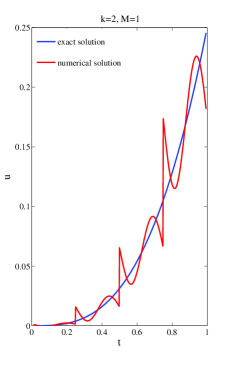
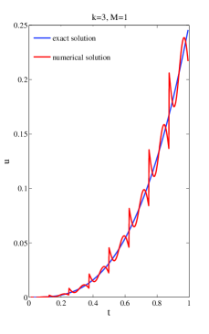
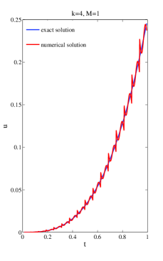
Figure 1: The comparison between exact and approximate solutions when $\alpha=0.2$, $x=0.5$.

Table 1: The absolute errors with $\alpha=0.2$ and various $k$, $M$ at $t=0.25$ for Example 6.1

x	$k=2$, $M=1$	$k=3$, $M=1$	$k=4$, $M=1$	$k=5$, $M=1$
0.1	4.7632e-04	1.7111e-04	7.1433e-05	3.2587e-05
0.2	1.9030e-03	6.8340e-04	2.8502e-04	1.2976e-04
0.3	4.2801e-03	1.5368e-03	6.4075e-04	2.9153e-04
0.4	7.6074e-03	2.7315e-03	1.1386e-03	5.1787e-04
0.5	1.1885e-02	4.2672e-03	1.7787e-03	8.0880e-04
0.6	1.7113e-02	6.1441e-03	2.5608e-03	1.1643e-03
0.7	2.3291e-02	8.3621e-03	3.4851e-03	1.5844e-03
0.8	3.0419e-02	1.0921e-02	4.5515e-03	2.0690e-03
0.9	3.8498e-02	1.3821e-02	5.7600e-03	2.6182e-03

Example 6.2 Let $a(x)=x$, $b(x)=-1$, $\ell=1$, and the initial-boundary values $y(x,0)=x-x^{3}$, $y(0,t)=y(\ell,t)=0$. The forcing term and exact solution are

$$f(x,t)=\frac{\Gamma(1+2\alpha)}{\Gamma(1+\alpha)}t^{\alpha}(x-x^{3})+(1+t^{2\alpha})(7x-3x^{3}),$$

and $y(x,t)=(1+t^{2\alpha})(x-x^{3})$, respectively. The code is run with $p=1$. Fig. 2 gives the numerical solutions for $\alpha=0.5$, $\alpha=0.9$ by using $k=4$, $M=1$, and $N_{h}=40$. Table 2 reports the absolute errors at $t=0.5$ for various $k$, $M$ with $\alpha=0.7$ and $N_{h}=10$. It is seen that our method is well convergent.

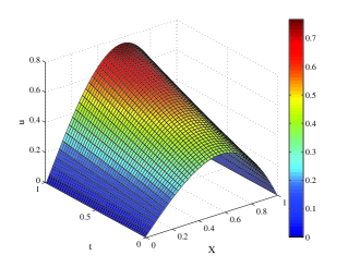
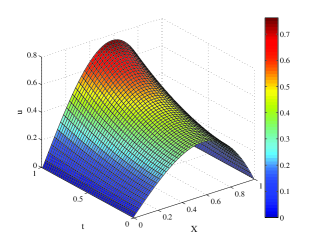
Figure 2: The numerical solutions with $k=4$, $M=1$, $N_{h}=40$ for $\alpha=0.5$ and $\alpha=0.9$.

Table 2: The absolute errors with $\alpha=0.7$ and various $k$, $M$ at $t=0.5$ for Example 6.2

x	$k=4$, $M=1$	$k=5$, $M=2$	$k=6$, $M=1$	$k=7$, $M=2$
0.1	3.3203e-03	1.6340e-03	8.0029e-04	3.8732e-04
0.2	6.4390e-03	3.1686e-03	1.5517e-03	7.5082e-04
0.3	9.1546e-03	4.5045e-03	2.2055e-03	1.0667e-03
0.4	1.1266e-02	5.5425e-03	2.7130e-03	1.3114e-03
0.5	1.2571e-02	6.1836e-03	3.0257e-03	1.4615e-03
0.6	1.2870e-02	6.3291e-03	3.0955e-03	1.4938e-03
0.7	1.1961e-02	5.8808e-03	2.8746e-03	1.3855e-03
0.8	9.6461e-03	4.7409e-03	2.3158e-03	1.1146e-03
0.9	5.7250e-03	2.8126e-03	1.3728e-03	6.5958e-04

Example 6.3 In this test, we consider Eqs. (1)-(3) with $a(x)=1$, $b(x)=-x$, $\ell=1$, and the initial-boundary values $y(x,0)=x^{3}$, $y(0,t)=0$, $y(\ell,t)=1+t^{2}$, and the forcing function

$$f(x,t)=\frac{2t^{2-\alpha}x^{3}}{\Gamma(3-\alpha)}-3(1+t^{2})x^{2}.$$

The exact solution is given by $y(x,t)=(1+t^{2})x^{3}$. In Fig. 3, we depict the global errors versus the variation of parameter $p$ for $\alpha=0.3$, $\alpha=0.6$ with $k=6$, $M=1$, and $N_{h}=20$. As the graph show, the optimal $p$ for this problem is roughly located on $[0.002,0.005]$. On taking $p=0.025$, the numerical solutions for $\alpha=0.1$ computed by using $k=3$, $M=1$, $N_{h}=20$ and $k=4$, $M=1$, $N_{h}=40$ are displayed in Fig. 4, and some numerical results at $t=t_{N_{t}}$ with $k=6$, $M=2$ are tabulated in Table 3, where the second-order convergent rates and good accuracy are observed and confirmed.

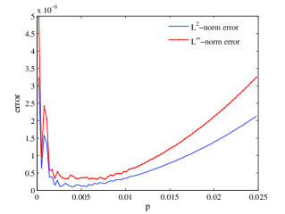
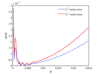
Figure 3: The global errors versus the variation of $p$ with $k=6$, $M=1$, $N_{h}=20$ for $\alpha=0.3$ and $\alpha=0.6$.

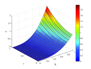
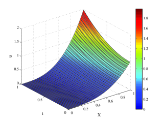
Figure 4: The numerical solutions with $k=3$, $M=1$, $N_{h}=20$ and $k=4$, $M=1$, $N_{h}=40$ for $\alpha=0.1$.

Table 3: The numerical results with $k=6$, $M=2$ and various $\alpha$ at $t=t_{N_{t}}$ for Example 6.3.

$\alpha$	$N_{h}$	$e_{2}(t_{N_{t}},N_{h})$	Cov. rate	$e_{\infty}(t_{N_{t}},N_{h})$	Cov. rate
$0.3$	5	3.4402e-07	-	5.0737e-07	-
	10	8.6712e-08	1.9882	1.3205e-07	1.9419
	20	2.1705e-08	1.9982	3.3023e-08	1.9996
	40	5.3797e-09	2.0125	8.2022e-09	2.0094
$0.6$	5	3.3183e-07	-	4.8881e-07	-
	10	8.3584e-08	1.9891	1.2771e-07	1.9364
	20	2.0960e-08	1.9956	3.2003e-08	1.9966
	40	5.2376e-09	2.0006	8.0132e-09	1.9978
$0.9$	5	3.1876e-07	-	4.6891e-07	-
	10	8.0489e-08	1.9856	1.2333e-07	1.9268
	20	2.0495e-08	1.9735	3.1339e-08	1.9765
	40	5.4419e-09	1.9131	8.3056e-09	1.9158

6 Conclusion

In this article, we have presented a numerical algorithm for the variable coefficient time-fractional convection-diffusion equation by approximating its solution as a truncated sine-cosine wavelets series in time and exponential spline interpolation in space. The method turns a differential model into a solvable algebraic system via the derived wavelet operational matrix of fractional integration and thereby is of significance to make the execution of program easier and more economic since the historical correlation of these models. The tested results of its codes on some illustrative examples have manifested that it can handle the given equations very effectively. It is certain that our method provides an alternative to simulate the other fractional problems.

- (1) Bhrawy, A., Zaky, M.: A fractional-order Jacobi Tau method for a class of time-fractional PDEs with variable coefficients. Math. Method Appl. Sci. 39(7), 1765–1779 (2016)
- (2) Chen, Y.M., Wu, Y.B., Cui, Y.H., Wang, Z.Z., Jin, D.M.: Wavelet method for a class of fractional convection-diffusion equation with variable coefficients. J. Comput. Sci. 1(3), 146–149 (2010)
- (3) Diethelm, K., Ford, N.J., Freed, A.D.: A predictor-corrector approach for the numerical solution of fractional differential equations. Nonlinear Dynam. 29(1-4), 3–22 (2002)
- (4) Ervin, V.J., Heuer, N., Roop, J.P.: Numerical approximation of a time dependent, nonlinear, space-fractional diffusion equation. SIAM J. Numer. Anal. 45(2), 572–591 (2007)
- (5) Esmaeili, S., Shamsi, M.: A pseudo-spectral scheme for the approximate solution of a family of fractional differential equations. Commun. Nonlinear Sci. Numer. Simul. 16(9), 3646–3654 (2011)
- (6) Gu, J.S., Jiang, W.S.: The Haar wavelets operational matrix of integration. Int. J. Syst. Sci. 27(7), 623–628 (1996)
- (7) Gu, Y.T., Zhuang, P., Liu, Q.: An advanced meshless method for time fractional diffusion equation. Int. J. Comp. Meth-Sing 8(4), 653–665 (2011)
- (8) Huang, C.B., Yu, X.J., Wang, C., Li, Z.Z., An, N.: A numerical method based on fully discrete direct discontinuous Galerkin method for the time fractional diffusion equation. Appl. Math. Comput. 264(1), 483–492 (2015)
- (9) Izadkhah, M.M., Saberi-Nadjafi, J.: Gegenbauer spectral method for time-fractional convection-diffusion equations with variable coefficients. Math. Method Appl. Sci. 38(15), 3183–3194 (2015)
- (10) Ji, C.C., Sun, Z.Z.: A high-order compact finite difference scheme for the fractional sub-diffusion equation. J. Sci. Comput. 64(3), 959–985 (2015)
- (11) Jiang, Y.J., Ma, J.T.: High-order finite element methods for time-fractional partial differential equations. J. Comput. Appl. Math. 235(11), 3285–3290 (2011)
- (12) Kilicman, A., Al-Zhour, Z.A.A.: Kronecker operational matrices for fractional calculus and some applications. Appl. Math. Comput. 187(1), 250–265 (2007)
- (13) Koeller, R.C.: Applications of fractional calculus to the theory of viscoelasticity. J. Appl. Mech. 51(2), 299–307 (1984)
- (14) Li, C.P., Chen, A., Ye, J.J.: Numerical approaches to fractional calculus and fractional ordinary differential equation. J. Comput. Phys. 230(9), 3352–3368 (2011)
- (15) Lin, Y.M., Xu, C.J.: Finite difference/spectral approximations for the time-fractional diffusion equation. J. Comput. Phys. 225(2), 1533–1552 (2007)
- (16) Luo, W.H., Huang, T.Z., Wu, G.C., Gu, X.M.: Quadratic spline collocation method for the time fractional subdiffusion equation. Appl. Math. Comput. 276, 252–265 (2016)
- (17) Mainardi, F.: Fractals and Fractional Calculus Continuum Mechanics. Springer, Verlag (1997)
- (18) McCartin, B.J.: Theory of exponential splines. J. Approx. Theory 66(1), 1–23 (1991)
- (19) Momani, S., Odibat, Z.: A novel method for nonlinear fractional partial differential equations: Combination of DTM and generalized Taylor’s formula. J. Comput. Appl. Math. 220(1-2), 85–95 (2008)
- (20) Pirkhedri, A., Javadi, H.H.S.: Solving the time-fractional diffusion equation via Sinc-Haar collocation method. Appl. Math. Comput. 257, 317–326 (2015)
- (21) Podlubny, I.: Fractional Differential Equations. Academic Press, London (1999)
- (22) Saadatmandi, A., Dehghan, M., Azizi, M.R.: The Sinc-Legendre collocation method for a class of fractional convection-diffusion equations with variable coefficients. Commu. Nonlinear Sci. Numer. Simul. 17(11), 4125–4136 (2012)
- (23) Sayevand, K., Yazdani, A., Arjang, F.: Cubic B-spline collocation method and its application for anomalous fractional diffusion equations in transport dynamic systems. J. Vib. Control 22(9), 2173–2186 (2016)
- (24) Sweilam, N.H., Khader, M.M., Al-Bar, R.F.: Numerical studies for a multi-order fractional differential equation. Phys. Lett. A 371(1-2), 26–33 (2007)
- (25) Uddin, M., Haq, S.: RBFs approximation method for time fractional partial differential equations. Commu. Nonlinear Sci. Numer. Simul. 16(11), 4208–4214 (2011)
- (26) Yi, M.X., Huang, J., Wei, J.X.: Block pulse operational matrix method for solving fractional partial differential equation. Appl. Math. Comput. 221, 121–131 (2013)
- (27) Zhuang, P.H., Liu, F.W.: Implicit difference approximation for the time fractional diffusion equation. J. Comput. Appl. Math. 22(3), 87–99 (2006)