The entropy of a classical thermally isolated Hamiltonian system is given by the logarithm of the measure of phase space enclosed by the constant energy hyper-surface, also known as volume entropy. It has been shown that on average the latter cannot decrease if the initial state is sampled from a classical passive distribution. Quantum extension of this result has been shown, but only for systems with a non-degenerate energy spectrum. Here we further extend to the case of possible degeneracies.
1 Introduction
Since the birth of statistical mechanics, it has been recognised that the logarithm of the volume of phase space enclosed by the constant energy surface of a classical thermally isolated systems (the so called volume entropy), is a good expression for its thermodynamic entropy. The mathematical and physical foundation of the volume entropy have been addressed various times in the history of statistical physics [1, 2, 3, 4, 5, 6, 7, 8, 9, 10, 11, 12, 13] and is currently the object of further investigation [14, 15, 16, 17].
One property of the volume entropy that matches the corresponding property of thermodynamic entropy is that, when the adiabatic theorem holds, it remains constant in time [4, 8]. The question then naturally arises of what happens to the volume entropy when the adiabatic theorem does not hold, e.g., if the timescale of variation of is not slow compared to the timescales in the system. Is it increasing as one expects for the thermodynamic entropy? A positive answer to this question has been given in [18] in a statistical sense. If the initial state is sampled randomly from a passive distribution [i.e., a distribution of the form , with a monotonic decreasing function, and the Hamiltonian at initial time], then the statistical expectation of the volume entropy at a time is larger than its initial expectation value.
A second question that arises regards how to extend the notion of volume entropy to the quantum case. The answer is not unique and at least two proposals exist in the literature. One proposal defines the quantum counterpart of the phase space volume as [14]. The other defines a “number operator” as that operator whose eigenvectors are the Hamiltonian eigenvectors and whose eigenvalues are the corresponding labels , that order the the eigen-energies in increasing fashion . The “volume entropy operator” is then the logarithm of the “number operator”[18, 19, 20]. An advantage of the latter definition is that it allows for a generalisation of the classical results mentioned above. A drawback is that it applies to systems with non-degenerate spectra only, thus excluding interesting physical scenarios, e.g. the joining of two identical systems [21], or their disjoining. The purpose of this work is accordingly to extend the notion of “volume entropy operator” to possibly degenerate spectra and to investigate its behaviour under a generic, non-necessarily adiabatic, quantum evolution.
2 Quantum volume entropy in presence of degenerate eigenenergies
We consider the entropy associated to a thermally isolated classical Hamiltonian system, with a parameter () dependent Hamiltonian in the expression given by Gibbs [3]:
(1)
where denotes the measure of the portion of phase space which at fixed parameter has energy below : , [22]. As mentioned it is an adiabatic invariant [4, 8], and when the adiabatic theorem is not satisfies, on average it cannot decrease if the initial state is sampled randomly from a classical passive distribution [i.e., a distribution of the form , with a monotonic decreasing function, here is the value taken by at time ].
An analogous result has been proven for quantum mechanical systems with non-degenerate spectrum in [18, 19]. The quantum mechanical treatment requires the introduction of a quantum mechanical counterpart of the classical volume . One possible choice is to consider the operator [18, 19, 20]
(2)
where is the dimension of the Hilbert space, denote the eigenvectors of the -dependent Hamilton operator
(3)
The spectrum is assumed to be non degenerate for all ’s, and the eigenvalues are ordered in an increasing fashion:
(4)
Accordingly, the expectation of the “number operator” on an energy eigenstate gives the ordering label , saying how many eigenstates exist with energy not above . This is in analogy with the quantity roughly saying how many shells of some unit measure exist at some fixed below the shell of energy . One defines accordingly the entropy operator as follows
(5)
Consider now the case when changes in time according to a time dependent protocol
(6)
The time dependent Hamiltonian generates a unitary evolution according to the Schrödinger equation
(7)
Consider an initial state and its evolved , and consider the expectation of the volume entropy operator at time
Let , , be two probability distributions. Let for .
Let be a non-decreasing real sequence. If there exists a doubly stochastic matrix with elements such that , then
(10)
The thesis of Theorem 1 follows by writing and and by noticing that the population of state at time is linked to the initial population by the expression where the quantum mechanical transition probabilities
form a doubly stochastic matrix.
Note that the non-degeneracy condition implies that no level crossing occurs during the dynamics. This implies that under the further condition of a slow driving the quantum adiabatic theorem [24] applies. In that case the inequality (9) turns into an equality.
In case the spectrum has possibly some degeneracies at a given
we order the eigenenergies in a non-decreasing fashion
(11)
Note the sign, accounting for the possibility that two or more states have the same energy. Let
(12)
be the set of all indices such that for a given the corresponding energy is equal to . Let , be its cardinality, namely the degree of degeneracy of the energy eigenvalue . Let be accordingly the number of states with energy not above . In analogy with the non-degenerate case one can define the “number operator” as and the entropy operator as . From the physical point of view the latter definition would however present a problem. Imagine the system is at equilibrium in a statistical mixture at some fixed where same energy states are equally populated: if . Imagine all states are non-degenerate apart from states , which are doubly degenerate. It is , and . Imagine now that an infinitesimal perturbation lifts the degeneracy, so that we have the new numbers , . While the populations and would be affected at most by terms of , the expectation of would change by the finite amount . We regard such finite jump associated to an arbitrarily small perturbation as unphysical. A definition of “volume entropy operator” that does not suffer from the degeneracy-lift issue is the following:
(13)
where
(14)
is the geometric average of over the set . Accordingly
is the arithmetic average of over the set . Note that in the case of a non-degenerate spectrum it is and one recovers the definition in Eq. (5).
With the definitions in (13,14) we can state the following
Theorem 2
Let for and all times .
If there exist a probability distribution such that , for and
then
(15)
Proof.
We first prove the thesis by assuming that at time the spectrum is non-degenerate, i.e. . It is .
Due to the assumption it is .
On the other hand . Since with forming a doubly stochastic matrix the thesis follows from Lemma 1.
Let us now consider the case when the spectrum at time possibly have degeneracies. Let us imagine for illustrative proposes that all states are non-degenerate apart from states , which are doubly degenerate. Their contribution to is . We can re-express that as , where . More generally, in case of many degenerate subspaces of arbitrary dimension, by introducing the new probabilities
(16)
the final entropy expectation reads . It now remains to be demonstrated that the are linked to the by a doubly stochastic matrix.
Using vector notation , . It is where is a block diagonal matrix whose blocks are of the form
(21)
with the dimension of the block. In the various blocks have the dimension of the corresponding degenerate subspaces. Each block is doubly stochastic (the sum of the elements in any row or column is ),
and so is the matrix itself. Let be the matrix whose elements are the transition probabilities and let . It is . Then .
Since both and are doubly stochastic, so is their product that is
(22)
where are the elements of the doubly stochastic matrix . The thesis then follows from Lemma 1.
3 Example
As an example we consider the sudden breaking of a XX spin chain of length into two identical XX spin chains of length . Studies regarding the joining of such spin chains were reported in [21, 25].
The pre-breaking Hamiltonian reads
(23)
where , , , denoting the Pauli matrices of the -th spin.
The post-breaking Hamiltonian reads:
(24)
where
(25)
(26)
The Hamiltonians all represent XX spin chains of different lengths .
The spectrum of the full chain is given by
[26, 27]
(27)
where , denotes the occupation of each fermionic mode, and
(28)
is the corresponding energy. The final spectrum is accordingly given by
(29)
where , with denoting the occupation of each fermionic mode in the left chain, and denoting the occupation of each fermionic mode in the right chain. Besides possible accidental degeneracies, the final spectrum has further systematic degeneracies due to the exchange symmetry.
We assume an initial Gibbs preparation , with , that is:
(30)
where denotes the full chain eigenvectors.
Ordering the initial eigenvalues in increasing fashion, amounts to establish a bijective application
(31)
(32)
such that if . Such application is not unique because the spectrum has degeneracies. We define the sets
(33)
of all indexes corresponding to the energy . The pre-quench volume entropy operator reads accordingly
(34)
where
(35)
The pre-quench expectation of volume entropy operator is therefore
(36)
Similarly for the post-quench quantities with the symbol replaced by , and
(37)
with the final eignevectors.
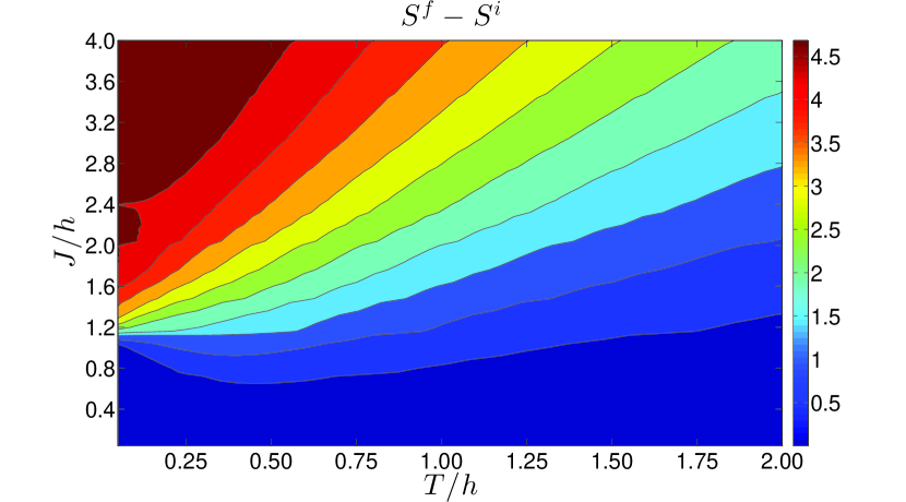
The explicit expression of the quantum mechanical transition probabilities is given in the appendix of Ref. [25]. With them we have computed and plotted the change in the expectation of the volume entropy operator as a function of and , for and fixed . This corresponds to a matrix of transition probabilities. The results are reported in Fig. 1. The computed values of are all non-negative in accordance with Theorem 2.
Figure 1: Change in the expectation of volume entropy operator for the sudden beak-up of a XX chain as a function of interaction strength and temperature .
4 Conclusion
We have extended the results of Ref. [18] to the case of possibly degenerate spectra, and have illustrated them using the break-up of a spin-chain as an example.
Ackowledgements
This research was supported by a Marie Curie Intra European Fellowship within the 7th European Community Framework Programme through the project NeQuFlux grant n. 623085 and by the COST action MP1209 “Thermodynamics in the quantum regime”.
References
References
[1]
Helmholtz H 1895 Wissenschaftliche Abhandlungen vol 3 ed Wiedemann G
(Leipzig: Johann Ambrosius Barth) pp 142–162, 163–178, 179–202
[2]
Boltzmann L 1909 über die eigenschaften monocyklischer und anderer damit
verwandter systeme Wissenschaftliche Abhandlungen vol 3 ed
Hasenöhrl F (Leipzig: Johann Ambrosius Barth Verlag) pp 122–152
[3]
Gibbs J 1902 Elementary Principles in Statistical Mechanics (New Haven:
Yale University Press)
[4]
Hertz P 1910 Ann. Phys. (Leipzig)338 225–274, 537–552
[5]
Einstein A 1911 Ann. Phys. (Leipzig)34 175
[6]
Schlüter A 1948 Z. Naturforsch. A3 350–360
[7]
Münster A 1969 Statistical Thermodynamics (Vol. 1) (Berlin:
Springer)
[8]
Berdichevsky V L 1997 Thermodynamics of Chaos and Order harlow, essex
ed (Addison-Wesley / Longman)
[9]
Pearson E M, Halicioglu T and Tiller W A 1985 Phys. Rev. A32
3030–3039
[10]
Adib A 2004 J. Stat. Phys.117 581–597
[11]
Campisi M 2005 Stud. Hist. Phil. Mod. Phys.36 275–290
[12]
Dunkel J and Hilbert S 2006 Physica A370 390–406
[13]
Campisi M and Kobe D H 2010 Am. J. Phys.78 608–615
[14]
Dunkel J and Hilbert S 2014 Nat. Phys.10 67–72
[15]
Hilbert S, Hänggi P and Dunkel J 2014 Phys. Rev. E90 062116