Estimating dimension of inertial manifold from unstable periodic orbits

Abstract

We provide numerical evidence that a finite-dimensional inertial manifold on which the dynamics of a chaotic dissipative dynamical system lives can be constructed solely from the knowledge of a set of unstable periodic orbits. In particular, we determine the dimension of the inertial manifold for Kuramoto-Sivashinsky system, and find it to be equal to the ‘physical dimension’ computed previously via the hyperbolicity properties of covariant Lyapunov vectors.

Dynamics in chaotic dissipative systems is expected to land, after a transient period of evolution, on a finite-dimensional object in state space called the inertial manifold Constantin et al. (1989); Temam (2013, 1990); Foias et al. (1988); Robinson (1995). This is true even for infinite-dimensional systems described by partial differential equations, and offers hope that their asymptotic dynamics may be represented by a finite set of ordinary differential equations, a drastically simplified description. The existence of a finite-dimensional inertial manifold has been established for systems such as the Kuramoto-Sivashinsky, the complex Ginzburg-Landau, and some reaction-diffusion systems Temam (2013). For the Navier-Stokes flows its existence remains an open problem Temam (1990), but dynamical studies, such as the determination of sets of periodic orbits embedded in a turbulent flows Gibson et al. (2008); Willis et al. (2016), strengthen the case for a geometrical description of turbulence. However, while mathematical approaches may provide rigorous bounds on dimensions of inertial manifolds, a constructive description of inertial manifolds remains a challenge.

Recent progress towards this aim comes from the viewpoint of linearized stability analysis of spatio-temporally chaotic flows Yang et al. (2009); Takeuchi et al. (2011). Specifically, numerical investigations of the dynamics of covariant Lyapunov vectors, made possible by the algorithm developed in refs. Ginelli et al. (2007, 2013), have revealed that the tangent space of a generic spatially-extended dissipative system is split into two hyperbolically decoupled subspaces: a finite-dimensional subspace of “entangled” or “physical” Lyapunov modes (referred to in what follows as the “physical manifold”), which is presumed to capture all long-time dynamics, and the remaining infinity of transient (“isolated,” “spurious”) Lyapunov modes. Covariant Lyapunov vectors span the Oseledec subspaces Oseledec (1968); Eckmann and Ruelle (1985) and thus indicate the intrinsic directions of growth or contraction at every point on the physical manifold. The dynamics of the vectors that span the physical manifold is entangled, with frequent tangencies between them. The transient modes, on the other hand, are damped so strongly by the dissipation, that they are isolated - at no time do they couple by tangencies to the entangled modes that populate the physical manifold. In refs. Yang et al. (2009); Takeuchi et al. (2011) it was conjectured that the physical manifold provides a local linear approximation to the inertial manifold at any point on the attractor, and that the dimension of the inertial manifold is given by the number of the entangled Lyapunov modes. Further support for this conjecture was provided by ref. Yang and Radons (2012), which verified that the vectors connecting pairs of recurrent points –points on the chaotic trajectory far apart in time but nearby each other in state space– are confined within the local tangent space of the physical manifold.

These simulations of long time chaotic trajectories have been successful in establishing that the physical manifold, defined everywhere along a chaotic trajectory by locally flat tangent space, captures the finite dimensionality of the inertial manifold, but they do not tell us much about how this inertial manifold is actually laid out in state space.

In this letter, we go one important step further and show that the finite-dimensional physical manifold can be precisely embedded in its infinite-dimensional state space, thus opening a path towards its explicit construction. The key idea Cvitanović et al. (2016) is to populate the inertial manifold by an infinite hierarchy of unstable time-invariant solutions, such as periodic orbits, an invariant skeleton which, together with the local “tiles” obtained by linearization of the dynamics, fleshes out the physical manifold. Chaos can then be viewed as a walk on the inertial manifold, chaperoned by the nearby unstable solutions embedded in the physical manifold. Such unstable periodic orbits have already been used to compute global averages over chaotic dynamics, also for spatially-extended systems, such as the Kuramoto-Sivashinsky Christiansen et al. (1997); Lan and Cvitanović (2008); Cvitanović et al. (2010) and Navier-Stokes Gibson et al. (2008) spatiotemporally chaotic flows.

In principle there are infinitely many unstable orbits, and each of them possesses infinitely many Floquet modes. While in the example that we study here we do not have a detailed understanding of the organization of periodic orbits (their symbolic dynamics), we do have sufficiently many of them to be able to show that one only needs to consider a finite number of unstable orbits to tile the physical manifold to a reasonable accuracy. We also show, for the first time, that each local tangent tile spanned by the Floquet vectors of an unstable periodic orbit splits into a set of entangled Floquet modes and the remaining set of transient modes. Furthermore, we verify numerically that the entangled Floquet manifold coincides locally with the physical manifold determined by the covariant Lyapunov vectors approach.

Throughout this letter, we focus on the one-dimensional Kuramoto-Sivashinsky equation Kuramoto and Tsuzuki (1976); Sivashinsky (1977), chosen here as a prototypical dissipative partial differential equation that exhibits spatiotemporal chaos Cross and Hohenberg (1993); Holmes et al. (1996),

$$u_{t}+u_{x}u+u_{xx}+u_{xxxx}=0,\quad x\in[0,L],$$ (1)

with a real-valued ‘velocity’ field $u(x,t)$, and the periodic boundary condition $u(x,t)=u(x+L,t)$. Following ref. Cvitanović et al. (2010), we fix the size at $L=22$, which is small enough so that unstable orbits are still relatively easy to determine numerically, and large enough for the Kuramoto-Sivashinsky equation to exhibit essential features of spatiotemporal chaos Hyman and Nicolaenko (1986). Dynamical evolution traces out a trajectory in the $\infty$-dimensional state space, $\mathrm{\mathbf{x}}(t)=f^{t}(\mathrm{\mathbf{x}}(0)$), with $\mathrm{\mathbf{x}}(t)\equiv{}u(x,t)$, where the time-forward map $f^{t}$ is obtained by integrating $\dot{\mathrm{\mathbf{x}}}=\mathrm{\mathbf{v}}(\mathrm{\mathbf{x}})$ up to time $t$. The linear stability of the trajectory is described by the Jacobian matrix $J^{t}(\mathrm{\mathbf{x}}(0))=\partial\mathrm{\mathbf{x}}(t)/\partial\mathrm{\mathbf{x}}(0)$, obtained by integrating $\dot{J}=A\,J$, where $A$ is the stability matrix $A(\mathrm{\mathbf{x}})=\partial\mathrm{\mathbf{v}}(\mathrm{\mathbf{x}})/\partial\mathrm{\mathbf{x}}$ . We integrate the system (1) numerically, by a pseudo-spectral truncation Cox and Matthews (2002); Kassam and Trefethen (2005) of $u(x,t)=\sum_{k=-\infty}^{+\infty}a_{k}(t)e^{iq_{k}x}\,,\;q_{k}=2\pi\,k/L$ to a finite number of Fourier modes. For the numerical accuracy required here we found $31$ Fourier modes (62-dimensional state space) sufficient. All orbits used here are found by a multiple shooting method and the Levenberg-Marquardt algorithm (see ref. Cvitanović et al. (2010) for details). A high accuracy computation of all Floquet exponents and vectors for this finite-dimensional state space (the key to all numerics presented here) has been made possible by the algorithm recently developed in ref. Ding and Cvitanović (2016). In our analysis, we use 200 pre-periodic orbits $\overline{ppo}_{{T_{p}}}$ and 200 relative periodic orbits $\overline{rpo}_{{T_{p}}}$, labelled by their periods ${T_{p}}$. These are the shortest period orbits taken from the set of over 60 000 determined in ref. Cvitanović et al. (2010) by near-recurrence searches. The method preferentially finds orbits embedded in the long-time attracting set, but offers no guarantee that all orbits up to a given period have been found.

The system is invariant under the Galilean transformations $u(x,t)\to{}u(x-ct,t)+c$, reflection $u(x,t)\to-u(-x,t)\equiv\sigma\,u(x,t)$, and spatial translations $u(x,t)\to{}u(x+\ell,t)\equiv{}g(\theta)\,u(x,t)$, where $\theta=2\pi\ell/L$, and ${\sigma}$ is the reflection operator. The Galilean symmetry is reduced by setting the mean velocity $\int\!dx\,u(x,t)$, a conserved quantity, to zero. Due to the $\textrm{O}(2)$ equivariance of Eq. (1), this system can have two types of ‘relative’ recurrent orbits (referred to collectively as “orbits” in what follows): pre-periodic orbits $u(x,0)={\sigma}u(x,{T_{p}})$ and relative periodic orbits $u(x,0)=g(\theta_{p})\,u(x,{T_{p}})$, where $g(\theta_{p})$ is the spatial translation by distance $\ell_{p}=L\theta_{p}/2\pi$. They are fixed points of maps ${\sigma}f^{{T_{p}}}$ and $g(\theta_{p})f^{{T_{p}}}$, respectively. Their Floquet multipliers $\Lambda_{j}$ and vectors $\bm{e}_{j}(\mathrm{\mathbf{x}})$ are the eigenvalues and eigenvectors of Jacobian matrix $J_{p}={\sigma}J^{{T_{p}}}$ or $J_{p}=g(\theta_{p})J^{{T_{p}}}$ for pre-periodic or relative periodic orbits, respectively. The Floquet exponents $\lambda_{j}$ (if complex, we shall only consider their real parts, with multiplicity 2) are related to multipliers by $\lambda_{j}=\ln|\Lambda_{j}|/{T_{p}}$. For an orbit $(\lambda_{j},\bm{e}_{j})$ denotes the $j$th Floquet (exponent, vector); for a chaotic trajectory it denotes the $j$th Lyapunov (exponent, vector).

Figure 1: (Color online) (a) Floquet exponents for $\overline{ppo}_{10.25}$ (circles), $\overline{rpo}_{16.31}$ (squares), and Lyapunov exponents of a chaotic trajectory (crosses). The inset shows a close-up of the 8 leading exponents. The number of the vanishing exponents is always two. Fourth Lyapunov exponent is small but strictly negative, $\lambda_{4}=-0.003$. (b) Time series of local Floquet exponents $\lambda_{j}(\mathrm{\mathbf{x}}(t))$ for $\overline{ppo}_{10.25}$. (c) Close-up of (b) showing the 8 leading exponents. Dashed lines indicate degenerate exponent pairs corresponding to complex Floquet multipliers.

Fig. 1 (a) shows the Floquet exponents spectra for the two shortest orbits, $\overline{ppo}_{10.25}$ and $\overline{rpo}_{16.31}$, overlaid on the Lyapunov exponents computed from a chaotic trajectory. The basic structure of this spectrum is shared by all 400 orbits used in our study Kaz (a). For chaotic trajectories, hyperbolicity between an arbitrary pair of Lyapunov modes can be characterized by a property called the domination of Oseledec splitting (DOS) Pugh et al. (2004); Bochi and Viana (2004). Consider a set of finite-time Lyapunov exponents

$$\lambda_{j}^{\tau}(\mathrm{\mathbf{x}})\equiv\frac{1}{\tau}\ln||J^{\tau}(\mathrm{\mathbf{x}})\bm{e}_{j}(\mathrm{\mathbf{x}})||\,,$$ (2)

with $L^{2}$ normalization $||\bm{e}_{j}(\mathrm{\mathbf{x}})||=1$. A pair of modes $j<\ell$ is said to fulfill ‘DOS strict ordering’ if $\lambda_{j}^{\tau}(\mathrm{\mathbf{x}})>\lambda_{\ell}^{\tau}(\mathrm{\mathbf{x}})$ along the entire chaotic trajectory, for $\tau$ larger than some lower bound $\tau_{0}$. Then this pair is guaranteed not to have tangencies Pugh et al. (2004); Bochi and Viana (2004). For chaotic trajectories, DOS turned out to be a useful tool to distinguish entangled modes from hyperbolically decoupled transient modes Yang et al. (2009); Takeuchi et al. (2011). Periodic orbits are by definition the infinite-time orbits ($\tau$ can be any repeat of ${T_{p}}$), so generically all nondegenerate pairs of modes fulfill DOS. Instead, we find it useful to define, by analogy to the ‘local Lyapunov exponent’ Bosetti and Posch (2014), the ‘local Floquet exponent’ as the action of the strain rate tensor Landau and Lifshitz (1959) $2\,D(\mathrm{\mathbf{x}})={A(\mathrm{\mathbf{x}})}{}^{\top}+A(\mathrm{\mathbf{x}})$ (where $A$ is the stability matrix) on the normalized $j$th Floquet eigenvector,

$$\lambda_{j}(\mathrm{\mathbf{x}})={\bm{e}_{j}(\mathrm{\mathbf{x}})}{}^{\top}D(\mathrm{\mathbf{x}})\,\bm{e}_{j}(\mathrm{\mathbf{x}})=\lim_{\tau\rightarrow 0}\lambda_{j}^{\tau}(\mathrm{\mathbf{x}})\,.$$ (3)

We find that time series of local Floquet exponents $\lambda_{j}(\mathrm{\mathbf{x}}(t))$ indicate a decoupling of the leading ‘entangled’ modes from the rest of the strictly ordered, strongly negative exponents [fig. 1 (b) and (c)]. Perhaps surprisingly, for every one of the 400 orbits we analyzed, the number of the entangled Floquet modes was always 8, equal to the previously reported number of the entangled Lyapunov modes for this system Yang and Radons (2012); Kaz (a). This leads to our first surmise: (1) each individual orbit embedded in the attracting set carries enough information to determine the dimension of the physical manifold.

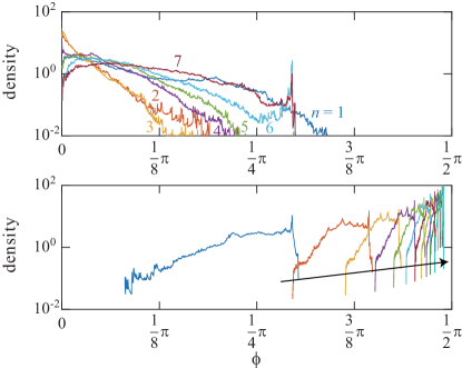
Figure 2: (Color online) A histogram of the principal angles $\phi$ between $S_{n}$ (the subspace spanned by the $n$ leading Floquet vectors) and $\bar{S}_{n}$ (the subspace spanned by the remaining $d-n$ Floquet vectors), accumulated over the 400 orbits used in our analysis. (top panel) For $n=1,2,\cdots,7$ ($S_{n}$ within the entangled manifold) the angles can be arbitrarily small. (bottom panel) For $n=8,10,12,\cdots,28$ (in the order of the arrow), for which all entangled modes are contained in $S_{n}$, the angles are bounded away from unity.

For an infinite-time chaotic trajectory, hyperbolicity can be assessed by measuring the distribution of minimal principal angles Björck and Golub (1973); Knyazev and Argentati (2002) between any pair of subspaces spanned by Lyapunov vectors Ginelli et al. (2007); Yang et al. (2009); Takeuchi et al. (2011). Numerical work indicates that as the entangled and transient modes are hyperbolically decoupled, the distribution of the angles between these subspaces is bounded away from zero, and that observation yields a sharp entangled-transient threshold.

This strategy cannot be used for individual orbits, as each one is of a finite period, and the minimal principal angle reached by a pair of Floquet subspaces remains strictly positive. Instead, we measure the angle distribution for a collection of orbits, and find that the entangled-transient threshold is as sharp as for a long chaotic trajectory: fig. 2 shows the principal angle distribution between two subspaces $S_{n}$ and $\bar{S}_{n}$, with $S_{n}$ spanned by the leading $n$ Floquet vectors and $\bar{S}_{n}$ by the rest. As in the covariant Lyapunov vectors analysis of long chaotic trajectories Yang et al. (2009), the distributions for small $n$ indicate strictly positive density as $\phi\to 0$. In contrast, the distribution is strictly bounded away from zero angles for $n\geq 8$, the number determined above by the local Floquet exponents analysis. This leads to our second surmise: (2) The distribution of principal angles for collections of periodic orbits enables us to identify a finite set of entangled Floquet modes, the analogue of the chaotic trajectories’ entangled covariant Lyapunov vector modes.

It is known, at least for low-dimensional chaotic attractors, that a dense set of periodic orbits constitutes the skeleton of a strange attractor Cvitanović et al. (2016). Chaotic trajectories meander around these orbits, approaching them along their stable manifolds, and leaving them along their unstable manifolds. If long-time trajectories are indeed confined to a finite-dimensional physical manifold, such shadowing events should take place within the subspace of entangled Floquet modes of the shadowed orbit. To analyze such shadowing, we need to measure the distances between the chaotic trajectories and the invariant orbits: the essential step here is symmetry reduction, i.e., replacement of a group orbit of states identical up to a symmetry transformation by a single state. Since translation $u(x,t)\to{}u(x+\ell,t)$ on a periodic domain implies a rotation $a_{k}(t)\to{}e^{iq_{k}\ell}a_{k}(t)$ in Fourier space, we choose to send both trajectories and orbits to the hyperplane $\operatorname{Im}(a_{1})=0,\operatorname{Re}(a_{1})>0$, called the first Fourier-mode slice Budanur et al. (2015), and measure the distances therein. This transformation reads

$$\hat{u}(x,t)=g(-\theta(t))u(x,t)$$ (4)

with $\theta(t)=\arg{}a_{1}(t)$. In the slice, both relative periodic orbits and pre-periodic orbits are reduced to periodic orbits. From Eq. (4), one easily finds how infinitesimal perturbations $\delta{}u(x,t)$ are transformed Kaz (b). This allows us to define the symmetry-reduced tangent space, with the in-slice perturbations $\delta\hat{u}(x,t)$, Jacobian matrix $\hat{J}^{t}(\hat{a})$, Floquet matrix $\hat{J}_{p}(\hat{a})$ and Floquet vectors $\hat{\bm{e}}_{j}(\hat{a})$. The dimension of the slice subspace is one less than the full state space: slice eliminates the marginal translational direction, while the remaining Floquet multipliers $\Lambda_{j}$ are unchanged by the transformation. Therefore, for the system studied here, there are only seven entangled modes, with one marginal mode (time invariance) in the in-slice description, instead of eight and two, respectively, in the full state space description. A shadowing of an orbit $u_{p}(x,t^{\prime})$ by a nearby chaotic trajectory $u(x,t)$ is then characterized by the in-slice separation vector

$$\Delta\hat{u}(x,t)\equiv\hat{u}(x,t)-\hat{u}_{p}(x,t_{p}),$$ (5)

where $t_{p}$ is chosen to minimize the in-slice distance $||\Delta\hat{u}||$.

Now we test whether the separation vector $\Delta{}\hat{u}(x,t)$ is confined to the tangent space spanned by the entangled in-slice Floquet vectors. To evaluate this confinement, one needs to take into account the nonlinearity of the stable and unstable manifolds for finite amplitude of $\Delta\hat{u}(x,t)$. We decompose the separation vector as

$$\Delta\hat{u}(x,t)=\hat{v}_{n}(x,t)+\hat{w}_{n}(x,t),$$ (6)

where $\hat{v}_{n}(x,t)$ is a vector in the subspace $\hat{S}_{n}$ spanned by the leading $n$ in-slice Floquet vectors and $\hat{w}_{k}(x,t)$ is in the orthogonal complement of $\hat{S}_{n}$. If $n$ is large enough so that $\hat{S}_{n}$ contains the local approximation of the inertial manifold, we expect $||\hat{w}_{n}||\sim||\hat{v}_{n}||^{2}\sim||\Delta\hat{u}||^{2}$ because of the smoothness of the inertial manifold; otherwise $||\hat{w}_{n}||$ does not vanish as $||\Delta\hat{u}||\to{}0$. In terms of the angle $\varphi_{n}$ between $\hat{S}_{n}$ and $\Delta\hat{u}$, $\sin\varphi_{n}\sim||\hat{w}_{n}||/||\hat{v}_{n}||\sim||\Delta\hat{u}||$ for $n$ above the threshold, while $\sin\varphi_{n}$ remains non-vanishing otherwise.

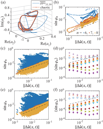
Figure 3: (Color online) (a) Shadowing event between a chaotic trajectory and $\overline{ppo}_{33.39}$, drawn over $2\,{T_{p}}$. (b) Parametric plot of $\sin\varphi_{n}(t)$ vs $||\Delta\hat{u}(x,t)||$ during the single shadowing event shown in (a), for $n=6,7,8$. (c) Same as (b), but a total of 230 shadowing events of $\overline{ppo}_{33.39}$ are used. (d) Average of $\sin\varphi_{n}$ collected from the 230 shadowing events, taken within each bin of the abscissa, for $n=4,5,6,7,9,11,17,21,25$ from top to bottom. (e)(f) Same as (c)(d), respectively, but for 217 shadowing events with $\overline{rpo}_{34.64}$. The dashed lines show $\sin\varphi_{n}\propto||\Delta\hat{u}||$ in all panels.

Following this strategy, we collected segments of a long-time chaotic trajectory during which it stayed sufficiently close to a specific orbit for at least one period of the orbit. Fig. 3 (a) illustrates such shadowing event with respect to $\overline{ppo}_{33.39}$. A parametric plot of $\sin\varphi_{n}(t)$ vs. $||\Delta\hat{u}(x,t)||$ during this event is shown in fig. 3 (b) for $n=6,7,8$ (blue circles, red squares, orange triangles, respectively). We can already speculate from such a single shadowing event that $\sin\varphi_{n}$ does not necessarily decrease with $||\Delta\hat{u}||$ for $n<7$, while it decreases linearly with $||\Delta\hat{u}||$ for $n\geq 7$. This threshold is clearly identified by accumulating data for all the recorded shadowing events with $\overline{ppo}_{33.39}$, fig. 3 (c): $\sin\varphi_{n}$ is confined below a line that depends linearly on $||\Delta\hat{u}||$ if and only if $n\geq 7$. We can see similarly clear separation in the average of $\sin\varphi_{n}$ taken within each bin of the abscissa [fig. 3 (d)]. This indicates that for $n<7$ (empty symbols), typical shadowing events manifest significant deviation of $\Delta\hat{u}$ from the subspace $\hat{S}_{n}$, whereas for $n\geq 7$ (solid symbols) $\Delta\hat{u}$ is always confined to $\hat{S}_{n}$. We therefore conclude that shadowing events are confined to the subspace spanned by the leading 7 in-slice Floquet vectors, or equivalently, by all the 8 entangled Floquet vectors in the full state space. The same conclusion was drawn for $\overline{rpo}_{34.64}$ [fig. 3 (e) and (f)] and five other orbits (not shown). We also verified that, when a chaotic trajectory approaches an orbit, the subspace spanned by all entangled Floquet modes of the orbit coincides with that spanned by all entangled Lyapunov modes of the chaotic trajectory. This implies our third surmise: the entangled Floquet manifold coincides locally with the entangled Lyapunov manifold, with either capturing the local structure of the inertial manifold.

In summary, we have used here the Kuramoto-Sivashinsky system to demonstrate by six independent calculations that the tangent space of a dissipative flow splits into entangled vs. transient subspaces, and to determine the dimension of its inertial manifold. The Lyapunov modes approach of refs. Ginelli et al. (2007); Yang et al. (2009); Yang and Radons (2012); Takeuchi et al. (2011); Kaz (a), applied here to Kuramoto-Sivashinsky on $L=22$ domain, identifies (1) the “entangled” Lyapunov exponents, by the dynamics of finite-time Lyapunov exponents, Eq. (2); and (2) the “entangled” tangent manifold, or “physical manifold,” by measuring the distributions of angles between covariant Lyapunov vectors. The Floquet modes approach Ding and Cvitanović (2016) developed here shows that (3) Floquet exponents of each individual orbit separate into entangled vs. transient, Fig. 1; (4) for ensembles of orbits, the principal angles between hyperplanes spanned by Floquet vectors separate the tangent space into entangled vs. transient, fig. 2; (5) for a chaotic trajectory shadowing a given orbit the separation vector lies within the orbit’s Floquet entangled manifold, fig. 3; and (6) for a chaotic trajectory shadowing a given orbit the separation vector lies within the chaotic trajectories covariant Lyapunov vectors’ entangled manifold.

All six approaches yield the same inertial manifold dimension, reported in earlier work Yang and Radons (2012); Kaz (a). The Floquet modes / unstable periodic orbits approach is constructive, in the sense that periodic points should enable us, in principle (but not attempted in this letter), to tile the global inertial manifold by local tangent spaces of an ensemble of such points. Moreover, and somewhat surprisingly, our results on individual orbits’ Floquet exponents, fig. 1 (b) and (c), and on shadowing of chaotic trajectories, fig. 3, suggest that each individual orbit embedded in the attracting set contains sufficient information to determine the entangled-transient threshold. However, the computation and organization of unstable periodic orbits is still a major undertaking, and can currently be carried out only for rather small computational domains Cvitanović et al. (2010); Willis et al. (2016). The good news is that the entangled Lyapunov modes approach Yang et al. (2009) suffices to determine the inertial manifold dimension, as Lyapunov modes calculations only require averaging over long chaotic trajectories, are much easier to implement, and can be scaled up to much larger domain sizes than $L=22$ considered here.

We hope the computational tools introduced in this letter can eventually contribute to solving outstanding issues of dynamical systems theory, such as the existence of an inertial manifold in the transitional turbulence regime of the Navier-Stokes equations, as well as to provide a practical guide to numerically accurate truncations of infinite-dimensional systems described by partial differential equations.