Optimal initial condition of passive tracers for their maximal mixing in finite time

Abstract

The efficiency of a fluid mixing device is often limited by fundamental laws and/or design constraints, such that a perfectly homogeneous mixture cannot be obtained in finite time. Here, we address the natural corollary question: Given the best available mixer, what is the optimal initial tracer pattern that leads to the most homogeneous mixture after a prescribed finite time? For ideal passive tracers, we show that this optimal initial condition coincides with the right singular vector (corresponding to the smallest singular value) of a suitably truncated Perron-Frobenius (PF) operator. The truncation of the PF operator is made under the assumption that there is a small length-scale threshold $\ell_{\nu}$ under which the tracer blobs are considered, for all practical purposes, completely mixed. We demonstrate our results on two examples: a prototypical model known as the sine flow and a direct numerical simulation of two-dimensional turbulence. Evaluating the optimal initial condition through this framework only requires the position of a dense grid of fluid particles at the final instance and their preimages at the initial instance of the prescribed time interval. As such, our framework can be readily applied to flows where such data is available through numerical simulations or experimental measurements.

1 Introduction

Given a fluid velocity field $\mathbf{u}(\mathbf{x},t)$, a passive tracer satisfies the linear advection equation

$$\partial_{t}\rho+\mathbf{u}\cdot\boldsymbol{\nabla}\rho=0,\quad\rho(\mathbf{x},t_{0})=f(\mathbf{x})$$ (1)

where the scalar field $\rho(\mathbf{x},t)$ denotes the concentration of the tracer at time $t$ and $f$ is its initial concentration at time $t_{0}$. Aref (1984) pointed out that laminar unsteady velocity fields can, over time, develop complex tracer patterns consisting of ever smaller scales. This observation has inspired the successful development of many stirring protocols to enhance mixing in engineered devices (see, e.g., Stroock et al. (2002); Gouillart et al. (2006); Mathew et al. (2007); Singh et al. (2008); Thiffeault et al. (2008); Gubanov and Cortelezzi (2010); Foures et al. (2014)).

Systematic classification of mixing efficiency of fluid flow, however, is relatively recent. This classification was initiated by Lin et al. (2011) who derived rigorous bounds on the mixing efficiency of velocity fields with a prescribed stirring energy or stirring power budget. A notable outcome of their program is the rather remarkable discovery of a finite-energy velocity field ($\|\mathbf{u}\|_{L^{2}}=const.<\infty$) that achieves perfect mixing in finite time (Lunasin et al., 2012). It was shown later, however, that any such velocity field must have infinite viscous dissipation, i.e. $\|\boldsymbol{\nabla}\mathbf{u}\|_{L^{2}}=\infty$ (Seis, 2013; Iyer et al., 2014).

Besides this fundamental limitation, the implementation of mathematically obtained optimal stirring strategies in a mixing device is not always feasible due to, for instance, geometric constraints. The problem is more acute in natural fluid flow (such as geophysical flows or the blood stream) over which we have virtually no control.

In light of the above discussion, the natural question is:

(Q) Given an unsteady velocity field, what is the optimal initial tracer pattern that leads to the most homogeneous mixture after a prescribed finite time?

In spite of its importance, this question has received relatively little attention. Hobbs and Muzzio (1997) carried out a case study where the effect of the tracer injection location in a Kenics mixer is examined. They find that, at least for short time horizons, the mixing efficiency depends significantly on the injection location. A similar case study is carried out by Gubanov and Cortelezzi (2009) who studied the mixing efficiency of five different initial tracer patterns in a two-dimensional nonlinear model, known as the sine flow.

Thiffeault and Pavliotis (2008) addressed an analogous question: the asymptotic mixing of passive tracers advected under a steady velocity field where the tracer is injected continuously into the flow via source terms. Through a variational approach, they determined the optimal distribution of the sources (also see Okabe et al. (2008), for related numerical results).

Here, we address the finite-time mixing of passive tracers advected by fully unsteady velocity fields, as formulated in (1). Specifically, we seek the optimal initial condition $f$ that leads to the most homogeneous mixture after a given finite time. To the best of our knowledge, a rigorous method for determining this optimal initial condition is missing.

Problem (Q) can, in principle, be formulated and solved as an infinite-dimensional optimization problem, where the optimal initial condition coincides with the minimizer of an appropriate cost functional. Such minimizers are typically obtained by iterative methods of adjoint-based optimization (Protas, 2008; Farazmand et al., 2011). This is, however, computationally prohibitive since it requires the backward-time integration of an adjoint partial differential equation (PDE) at each iteration.

Here, we show that under reasonable assumptions, the problem reduces to a finite-dimensional one that can be readily solved at a relatively low computational cost. To obtain this finite-dimensional reduction, we assume that tracer blobs smaller than a small, prescribed length-scale $\ell_{\nu}$ are considered completely mixed for all practical purposes. This assumption, that is made precise in Section 3, results in a natural Galerkin truncation of the Perron–Frobenius (PF) operator associated with the advection equation (1). We show that the optimal initial condition $f$ then coincides with a singular vector of the truncated PF operator.

Our results complement the transfer operator-based methods for detecting finite-time coherent sets in unsteady fluid flows (Froyland (2013); also see Dellnitz and Junge (1999); Froyland et al. (2007, 2010); Williams et al. (2015)). Coherent sets refer to subsets of the fluid which exhibit minimal deformation under advection and therefore inhibit efficient mixing of tracers with the surrounding fluid. Our aim here is the opposite, namely, initially large-scale structures that under advection deform mostly into small-scale filaments.

The remainder of the paper is organized as follows. In section 2, we introduce some basic notation and definitions. Section 3 contains our main results and section 4 details their numerical implementation. In section 5, the results are demonstrated on two examples.

2 Preliminaries

Consider an unsteady, incompressible velocity field $\mathbf{u}(\mathbf{x},t)$ defined over a bounded open subset $\mathcal{D}\subset\mathbb{R}^{d}$ where $d=2$ or $d=3$ for two- and three-dimensional flows, respectively. The trajectories $\mathbf{x}(t;t_{0},\mathbf{x}_{0})$ of the fluid particles satisfy the ordinary differential equation

$$\dot{\mathbf{x}}=\mathbf{u}(\mathbf{x},t),\quad t\in\mathbb{R},$$ (2)

where $\mathbf{x}(t;t_{0},\mathbf{x}_{0})$ denotes the time–$t$ position of the particle starting from the initial position $\mathbf{x}_{0}$ at time $t_{0}$. If the velocity field is sufficiently smooth, there exists a two-parameter family of homeomorphisms $\varphi_{s}^{t}$ (the flow map) such that $\mathbf{x}(t;s,\mathbf{x}_{0})=\varphi_{s}^{t}(\mathbf{x}_{0})$ for all times $t$ and $s$. As our interest here is in finite-time mixing, we restrict our attention to a prescribed finite time interval $[t_{0},t_{0}+T]$ of interest. The flow map $\varphi_{t_{0}}^{t_{0}+T}$ takes the initial position $\mathbf{x}_{0}$ of a fluid particle at time $t_{0}$ to its final position at time $t_{0}+T$. Since the finite time interval is fixed, we drop the dependence of the flow map on $t_{0}$ and $t_{0}+T$, and write $\varphi$ for notational simplicity.

Let $\rho(\mathbf{x},t)$ denote the concentration of a passive tracer, i.e. $\rho$ satisfies equation (1). Since the passive tracer is conserved along fluid trajectories, we have

$$\rho(\mathbf{x},t_{0}+T)=\rho(\varphi^{-1}(\mathbf{x}),t_{0})=f\circ\varphi^{-1}(\mathbf{x}),$$ (3)

for all $\mathbf{x}\in\mathcal{D}$. Note that since the flow map is a homeomorphisms, the inverse $\varphi^{-1}$ is well-defined. Equation (3) motivates the definition of the Perron-Frobenius (PF) operator.

Definition 1 (Perron–Frobenius operator).

The Perron–Frobenius operator associated with the flow map $\varphi:\mathcal{D}\to\mathcal{D}$ is the linear transformation $\mathcal{P}:L^{2}(\mathcal{D})\to L^{2}(\mathcal{D})$ such that, for all $f\in L^{2}(\mathcal{D})$,

$$(\mathcal{P}f)(\mathbf{x})=f\circ\varphi^{-1}(\mathbf{x}),\quad\forall\mathbf{x}\in\mathcal{D}.$$ (4)

The evolution of passive tracers can be described by the action of the PF operator on their initial conditions. More specifically, for the passive tracer $\rho$ described above, we have

$$\rho(\mathbf{x},t_{0}+T)=(\mathcal{P}f)(\mathbf{x}),$$ (5)

for all $\mathbf{x}\in\mathcal{D}$ (cf. equation (3)).

We point out that there is a more general definition of the PF operator applicable to non-invertible dynamics (see Definition 3.2.3 of Lasota and Mackey (1994)). In the special case where the flow map $\varphi$ is invertible and volume-preserving, the general definition is equivalent to Definition 4 above (Corollary 3.2.1 in Lasota and Mackey (1994); Froyland and Padberg (2009)).

For incompressible flow, the PF operator is a unitary transformation with respect to the $L^{2}(\mathcal{D})$ inner product $\langle\cdot,\cdot\rangle_{L^{2}}$. As a consequence, the $L^{2}$-norm $\|\rho(\cdot,t)\|_{L^{2}}$ of the tracer remains invariant under advection. Furthermore, the spatial average of the tracer is an invariant. Without loss of generality, one can assume that this spatial average vanishes, $\int_{\mathcal{D}}\rho(\mathbf{x},t)\mathrm{d}\mathbf{x}=0$ (Lin et al., 2011).

There has been several attempts to detect coherent structures in unsteady fluid flows using approximations of the PF operator (Froyland et al., 2007; Santitissadeekorn et al., 2010; Froyland et al., 2010). Froyland (2013) puts these approaches on a mathematically rigorous basis by composing the PF operator with diffusion operators. The resulting diffusive PF operator is compact and has a well-defined singular value decomposition (SVD). Froyland (2013) shows that a singular vector, corresponding to the largest non-unit singular value of the diffusive PF operator, can reveal minimally dispersive subsets of the fluid that remain coherent and thereby inhibit mixing (also see Froyland and Padberg-Gehle (2014)). Our goal here, however, is the opposite as we seek passive tracer initial conditions that mix most efficiently with their surrounding fluid.

3 Optimal initial conditions

3.1 Physical considerations

Given an initial tracer distribution, a reasonable mixer will generically deform the tracer through stretching and folding of material elements such that, over time, it develops ever smaller length scales. It is, therefore, desirable to release the tracer initially into smallest possible scales. In practice, the initially available range of scales into which the tracer may be released is limited to relatively large scales. We denote this large length-scale limit by $\ell_{I}$ (see figure 1, for an illustration). It is left then to the fluid flow to transform the initially large-scale blobs of tracer to small filaments through a stretch-and-fold mechanism.

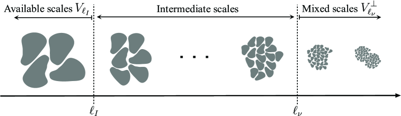
Figure 1: An illustration of the initially available scales (larger than $\ell_{I}$) and the mixed scales (smaller than $\ell_{\nu}$).

On the other hand, we assume that there is a small length scale threshold $\ell_{\nu}\ll\ell_{I}$, under which the tracer is considered, for all practical purposes, completely mixed. An efficient mixer, therefore, transfers the tracer distribution from large, initially available scales $\ell\geq\ell_{I}$ to the mixed scales $\ell<\ell_{\nu}$. In the next section, we make these statements precise.

3.2 Mathematical formulation

We consider a set of functions $\{\phi_{j}\}_{j\geq 1}$ forming a complete, orthonormal basis for the space of square integrable functions $L^{2}(\mathcal{D})$. That is $\langle\phi_{i},\phi_{j}\rangle_{L^{2}}=\delta_{ij}$ and for any $f\in L^{2}(\mathcal{D})$ there are constants $\alpha_{j}\in\mathbb{R}$ such that $\lim_{k\to\infty}\|f-\sum_{j=1}^{k}\alpha_{j}\phi_{j}\|_{L^{2}}=0$.

We also assume that there is a length scale $\ell_{j}$ associated to each function $\phi_{j}$, and that they are ordered such that the sequence $(\ell_{1},\ell_{2},\cdots)$ is decreasing. In other words, the length scale associated with the function $\phi_{j}$ decreases as $j$ increases. Such a basis can be taken, for instance, to be Fourier modes or wavelets (Walnut, 2013).

With this basis, we can mathematically model the subspace of initial conditions $V_{I}$. The subspace $V_{I}$ consists of all scalar functions $f$ whose smallest length scale is larger than or equal to $\ell_{I}$. Since the basis $\{\phi_{j}\}_{j\geq 1}$ is ordered, there is a positive integers $n$ such that

$$V_{I}=\mbox{span}\{\phi_{1},\phi_{2},\cdots,\phi_{n}\}=\{\mbox{Initially available length scales}\ \ell\geq\ell_{I}\}.$$ (6)

The subspace of unmixed length scales $V_{\nu}$ can be modeled similarly using a basis $\{\psi_{i}\}_{i\geq 1}$ for $L^{2}(\mathcal{D})$. We assume that this basis is also orthonormal, complete and associated with a decreasing sequence of length scales. The subspace $V_{\nu}$ consists of all scalar functions whose smallest length scale is larger than or equal to the unmixed length scale $\ell_{\nu}$. Therefore, there is $N\gg n$ such that

$$V_{\nu}=\mbox{span}\{\psi_{1},\psi_{2},\cdots,\psi_{N}\}=\{\mbox{Unmixed length scales}\ \ell\geq\ell_{\nu}\}.$$ (7)

Note that the bases $\{\psi_{i}\}_{i\geq 1}$ and $\{\phi_{i}\}_{i\geq 1}$ can be taken to be identical, but this is not necessary here.

We denote the orthogonal complement of $V_{\nu}$ by $V_{\nu}^{\perp}$. In terms of the basis functions, we have

$$V_{\nu}^{\perp}=\overline{\mbox{span}\{\psi_{N+1},\psi_{N+2},\cdots\}}=\{\mbox{Mixed length scales}\ \ell<\ell_{\nu}\},$$ (8)

where the overline denotes closure in the $L^{2}$ topology. The space $V_{\nu}^{\perp}$ consists of functions that only contain the mixed scales, that is scales smaller than $\ell_{\nu}$ (see figure 1).

3.3 Main result

Given an initial condition $f\in V_{I}$ for the tracer, its advected image $\mathcal{P}f\in L^{2}$ at the final time can potentially contain all length scales $\ell_{j}$. The flow redistributes the ‘energy’ budget of the tracer among various scales in such a way that the $L^{2}$-norm is conserved, i.e.,

$$\|f\|_{L^{2}}=\|\mathcal{P}f\|_{L^{2}}=\underbrace{\sum_{i=1}^{N}|\langle\mathcal{P}f,\psi_{i}\rangle_{L^{2}}|^{2}}_{\text{unmixed}}+\underbrace{\sum_{i=N+1}^{\infty}|\langle\mathcal{P}f,\psi_{i}\rangle_{L^{2}}|^{2}}_{\text{mixed}}.$$ (9)

A tracer is better mixed if more of its energy budget is transfered to the mixed scales $\ell<\ell_{\nu}$. Therefore, we seek optimal initial conditions $f\in V_{I}$ such that the energy budget of its image $\mathcal{P}f$ is mostly stored in the mixed scales, maximizing $\sum_{i=N+1}^{\infty}|\langle\mathcal{P}f,\psi_{i}\rangle|^{2}$. To make these statements more precise we introduce the following truncation of the PF operator.

Definition 2 (Truncated Perron–Frobenius operator).

We define the truncated PF operator $\mathcal{P}_{p}:V_{I}\to V_{\nu}$ as the linear map $\mathcal{P}_{p}=\Pi_{N}\circ\mathcal{P}$, where $\Pi_{N}$ is the orthogonal projection onto the $N$-dimensional subspace $V_{\nu}$. We also define the remainder operator $\mathcal{P}^{\perp}_{p}:V_{I}\to V_{\nu}^{\perp}$ as $\mathcal{P}^{\perp}_{p}=\mathcal{P}-\mathcal{P}_{p}$.

It follows from Parseval’s identity that $\|\mathcal{P}f\|_{L^{2}}^{2}=\|\mathcal{P}_{p}f\|_{L^{2}}^{2}+\|\mathcal{P}_{p}^{\perp}f\|_{L^{2}}^{2}$ (see equation (9)). The quantity $\|\mathcal{P}_{p}f\|_{L^{2}}^{2}$ represents the portion of the energy budget of the tracer that remains unmixed after advection to the final time $t_{0}+T$. The quantity $\|\mathcal{P}_{p}^{\perp}f\|_{L^{2}}^{2}$, on the other hand, represents the portion of the tracer that is completely mixed. We, therefore, seek initial conditions $f\in V_{I}$ that maximize the mixed energy budget $\|\mathcal{P}_{p}^{\perp}f\|_{L^{2}}^{2}$.

Since the truncated PF operator $\mathcal{P}_{p}$ is a linear transformation between finite-dimensional vector spaces $V_{I}$ and $V_{\nu}$, it can be represented by a matrix $P_{p}\in\mathbb{R}^{N\times n}$. More specifically, for any $f\in V_{I}$, there are scalars $\{\alpha_{1},\cdots,\alpha_{n}\}$ and $\{\beta_{1},\cdots,\beta_{N}\}$ such that

$$f=\sum_{j=1}^{n}\alpha_{j}\phi_{j}\quad\mbox{and}\quad\mathcal{P}_{p}f=\sum_{i=1}^{N}\beta_{i}\psi_{i}.$$ (10)

The matrix $P_{p}$ maps $\boldsymbol{\alpha}=(\alpha_{1},\cdots,\alpha_{n})^{\top}$ into $\boldsymbol{\beta}=(\beta_{1},\cdots,\beta_{N})^{\top}$, that is $\boldsymbol{\beta}=P_{p}\,\boldsymbol{\alpha}$. It follows from elementary linear algebra that the entries $[P_{p}]_{ij}$ of the matrix $P_{p}$ are given by

$$[P_{p}]_{ij}=\langle\mathcal{P}\phi_{j},\psi_{i}\rangle_{L^{2}},\quad i\in\{1,2,\cdots,N\},\quad j\in\{1,2,\cdots,n\}.$$ (11)

With this prelude, we can now state our main result.

Theorem 1.

Consider the function spaces $V_{I}$ and $V_{\nu}$ and their associated truncated PF operator defined above. The solution of

$$\arg\max\|\mathcal{P}_{p}^{\perp}f\|_{L^{2}},$$

with the maximum taken over all $f\in V_{I}$ with $\|f\|_{L^{2}}=1$, is given by $f_{\mbox{\tiny opt}}=\sum_{j=1}^{n}\alpha_{j}\phi_{j}$, where $\boldsymbol{\alpha}=(\alpha_{1},\alpha_{2},\cdots,\alpha_{n})^{\top}$ is a right singular vector of the truncated PF matrix (11) corresponding to its smallest singular value.

Proof.

Since $\|\mathcal{P}_{p}^{\perp}f\|_{L^{2}}^{2}=\|\mathcal{P}f\|_{L^{2}}^{2}-\|\mathcal{P}_{p}f\|_{L^{2}}^{2}=1-\|\mathcal{P}_{p}f\|_{L^{2}}^{2}$, maximizing $\|\mathcal{P}_{p}^{\perp}f\|_{L^{2}}^{2}$ is equivalent to minimizing $\|\mathcal{P}_{p}f\|^{2}$. Since $f$ belongs to the subspace $V_{I}$, the initial condition $f$ and its image $\mathcal{P}_{p}f$ can be expressed by the series (10) with $\boldsymbol{\beta}=P_{p}\,\boldsymbol{\alpha}$. Denoting the standard Euclidean norm by $|\cdot|$, we have $|\boldsymbol{\alpha}|^{2}=\|f\|_{L^{2}}^{2}=1$ and $|\boldsymbol{\beta}|^{2}=|P_{p}\,\boldsymbol{\alpha}|^{2}=\|\mathcal{P}_{p}f\|_{L^{2}}^{2}$. Therefore,

$$\min_{f\in V_{I},\|f\|=1}\|\mathcal{P}_{p}f\|_{L^{2}}=\min_{|\boldsymbol{\alpha}|=1}|P_{p}\,\boldsymbol{\alpha}|.$$ (12)

The minimum on the right hand side is well-known to coincide with the smallest singular value of the matrix $P_{p}$ (Stewart, 1998). The minimum is attained at the corresponding right singular vector of the matrix $P_{p}$. This completes the proof. ∎

Once the PF matrix $P_{p}$ is formed, the evaluation of the optimal initial condition $f_{\mbox{\tiny opt}}$, from the above theorem, is straightforward. We outline the computation of the truncated PF matrix $P_{p}$ in section 4.

Remark 1.

Note that if the matrix $P_{p}$ is not full-rank, there are initial conditions $f$ of the form (10) with $|\boldsymbol{\alpha}|=1$, such that $|P_{p}\,\boldsymbol{\alpha}|=0$. Such initial conditions result in ‘perfect mixing’ since their advected image $\mathcal{P}f$ belongs entirely to the mixed scales $\ell<\ell_{\nu}$, i.e., $\mathcal{P}f\in V_{\nu}^{\perp}$. In the examples studied in Section 5, such perfect finite-time mixing was not observed. In other words, the matrices $P_{p}$ are full-rank in these examples.

Remark 2.

We emphasize that the truncated PF operator $\mathcal{P}_{p}$ is not used as an approximation of the full PF operator $\mathcal{P}$. Instead, the truncation $\mathcal{P}_{p}$ followed naturally from the physical assumption that length scales $\ell<\ell_{\nu}$ are completely mixed. As is clear from equation (11), to evaluate the truncation $\mathcal{P}_{p}$, one still needs to utilize the full PF operator to evaluate the terms $\mathcal{P}\phi_{j}$.

4 Numerical implementation

Numerical computation of the optimal initial condition $f_{\mbox{\tiny opt}}$ relies on the scale-dependent bases $\{\phi_{i}\}_{i\geq 1}$ and $\{\psi_{i}\}_{i\geq 1}$. For completeness, we discuss two such bases: the Fourier basis and the Haar wavelet basis. Since the examples considered in Section 5 below are defined on equilateral two-dimensional domains, $\mathcal{D}=[0,L]\times[0,L]$, we focus on this special case. The generalization to the rectangular domain and to the three-dimensional case is straightforward.

4.1 Fourier basis

For periodic boundary conditions, it is natural to use the Fourier basis to define the spaces $V_{I}$ and $V_{\nu}$. The orthonormal Fourier basis associated with the two-dimensional domain $\mathcal{D}=[0,L]\times[0,L]$ consist of functions $(1/L)\exp\left[\mbox{i}(2\pi/L)(\mathbf{k}\cdot\mathbf{x})\right]$ where $\mathbf{k}\in\mathbb{Z}^{2}$ denotes the wave vector. The length scale associated to each Fourier mode is inversely proportional to the wave number, $|\mathbf{k}|\sim\ell^{-1}$. We take the space of available initial scalar fields to be the functions whose Fourier modes contain at most a prescribed wave number $k_{I}\sim\ell_{I}^{-1}$, i.e.,

$$V_{I}=\mbox{span}\left\{\frac{1}{L}\exp\left[\mbox{i}\frac{2\pi}{L}(\mathbf{k}\cdot\mathbf{x})\right]:\mathbf{k}=(k_{x},k_{y})\in\mathbb{Z}^{2},|k_{x}|\leq k_{I},|k_{y}|\leq k_{I}\right\}.$$ (13)

Similarly, the space of unmixed scales $V_{\nu}$ is the functions whose Fourier modes contain at most a prescribed wave number $k_{\nu}\sim\ell_{\nu}^{-1}\gg k_{I}$, i.e.,

$$V_{\nu}=\mbox{span}\left\{\frac{1}{L}\exp\left[\mbox{i}\frac{2\pi}{L}(\mathbf{k}\cdot\mathbf{x})\right]:\mathbf{k}=(k_{x},k_{y})\in\mathbb{Z}^{2},|k_{x}|\leq k_{\nu},|k_{y}|\leq k_{\nu}\right\}.$$ (14)

More generally, one could define the space $V_{I}$ (and similarly $V_{\nu}$) with independent upper bounds $k_{I_{x}}$ and $k_{I_{y}}$ on the wave-numbers $|k_{x}|$ and $|k_{y}|$, respectively. Since the domain is equilateral, and for simplicity, we choose the same upper bounds in both directions, $k_{I}=k_{I_{x}}=k_{I_{y}}$.

Since the tracer concentration is real-valued, the complex conjugate basis functions in $V_{I}$ and $V_{\nu}$ are redundant. Also, the basis with $\mathbf{k}=\mathbf{0}$ (corresponding to constant functions) is unnecessary since we assumed that the tracer has zero mean. Excluding these redundant functions, the effective dimension of the vector spaces $V_{I}$ and $V_{\nu}$ are $n=\dim V_{I}=2k_{I}(k_{I}+1)$ and $N=\dim V_{\nu}=2k_{\nu}(k_{\nu}+1)$, respectively.

4.2 Wavelet basis

While the above Fourier basis is a convenient choice, it restricts its applicability to the periodic boundary conditions. More general boundary conditions can be handled with an alternative basis, such as Haar wavelets. Such wavelet bases have the added advantage that they can be localized in space in addition to scale. This property renders wavelets particularly attractive in applications where the tracer can only be released into a subset of the fluid domain $\mathcal{D}$ due to geometric or design constraints. Contrast this with the global nature of the Fourier basis.

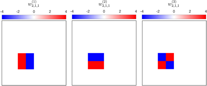
Figure 2: Three examples of the wavelet functions (17c) with $j=2$, $i_{x}=i_{y}=1$. The domain is $\mathcal{D}=[0,1]\times[0,1]$

Here, we consider the Haar wavelet basis. For completeness, we briefly review the construction of this basis in two dimensions. Denote the one-dimensional Haar scaling function with $s(x)=\mathds{1}_{[0,1)}(x)$ and the corresponding wavelet with $h(x)=\mathds{1}_{[0,1/2)}(x)-\mathds{1}_{[1/2,1)}(x)$ where $\mathds{1}_{A}$ is the indicator function of the set $A$. By dilations and translations, we obtain

$$s_{j,i}(x)=2^{j/2}s\left(2^{j}\frac{x}{L}-i\right),\quad j\geq 0,\quad i\in\{0,1,\cdots,2^{j}-1\},$$ (15a)

$$h_{j,i}(x)=2^{j/2}h\left(2^{j}\frac{x}{L}-i\right),\quad j\geq 0,\quad i\in\{0,1,\cdots,2^{j}-1\},$$ (15b)

where $0\leq x\leq L$ for a domain of size $L$. The collection of the wavelets $h_{j,i}$ forms an orthogonal basis for mean-zero functions in $L^{2}([0,L])$ (Daubechies, 1992). The integer $j$ determines the size of the support of $h_{j,i}$ (or $s_{j,i}$) which is $L\times 2^{-j}$. Since the wavelets with larger $j$ resolve finer structures (or smaller length scales), the integer $j$ is referred to as the scale of the wavelet. The integer $i$, on the other hand, introduces a translation in the support of each wavelet, introducing a space dependence at each scale $j$.

The functions $s_{j,i}$ and $h_{j,i}$ serve as the building blocks of multidimensional wavelet bases (Daubechies, 1992; Farge et al., 1999). For instance, a complete orthonormal basis for mean-zero functions in $L^{2}(\mathcal{D})$, with $\mathcal{D}=[0,L]\times[0,L]$, is formed by the set of functions

$$\big{\{}w^{(\mu)}_{j,i_{x},i_{y}}:\ 1\leq\mu\leq 3,\ 0\leq j,\ 0\leq i_{x}\leq 2^{j}-1,\ 0\leq i_{y}\leq 2^{j}-1\big{\}},$$ (16)

where

$$w_{j,i_{x},i_{y}}^{(1)}(x,y)=\frac{1}{L}h_{j,i_{x}}(x)s_{j,i_{y}}(y),$$ (17a)

$$w_{j,i_{x},i_{y}}^{(2)}(x,y)=\frac{1}{L}s_{j,i_{x}}(x)h_{j,i_{y}}(y),$$ (17b)

$$w^{(3)}_{j,i_{x},i_{y}}(x,y)=\frac{1}{L}h_{j,i_{x}}(x)h_{j,i_{y}}(y).$$ (17c)

The prefactor $1/L$ ensures that each basis function is of unit norm. The integer $j$ determine the scale in both $x$ and $y$ directions, while the integers $i_{x}$ and $i_{y}$ introduce the corresponding translations. Figure 2 shows three examples of the two-dimensional wavelet functions (17c) with $j=2$. The construction of two-dimensional wavelet bases from one-dimensional wavelets is not unique. For an alternative wavelet basis see, e.g., Chapter 10 of Daubechies (1992).

Using the wavelet basis (16), we define the subspace of initial conditions $V_{I}$ as

$$V_{I}=\mbox{span}\big{\{}w^{(\mu)}_{j,i_{x},i_{y}}:\ 1\leq\mu\leq 3,\ 0\leq j\leq J_{I}-1$$

$$0\leq i_{x}\leq 2^{j}-1,\ 0\leq i_{y}\leq 2^{j}-1\big{\}},$$ (18)

where the integer $J_{I}$ sets the initially available length scales. Roughly speaking, the wavelet subspace $V_{I}$ contains tracer blobs of size $\ell_{I}=L\times 2^{-J_{I}}$ or larger. Similarly, we define the subspace of unmixed length scales by

$$V_{\nu}=\mbox{span}\big{\{}w^{(\mu)}_{j,i_{x},i_{y}}:\ 1\leq\mu\leq 3,\ 0\leq j\leq J_{\nu}-1$$

$$0\leq i_{x}\leq 2^{j}-1,\ 0\leq i_{y}\leq 2^{j}-1\big{\}},$$ (19)

containing the unmixed tracer blobs of size $\ell_{\nu}=L\times 2^{-J_{\nu}}$ or larger. For given positive integers $J_{I}$ and $J_{\nu}$, we have $n=\dim V_{I}=4^{J_{I}}-1$ and $N=\dim V_{\nu}=4^{J_{\nu}}-1$.

Recall that the basis functions $\phi_{i}$ spanning the domain $V_{I}$ of the truncated PF operator $\mathcal{P}_{p}$ need not to be identical to the basis functions $\psi_{i}$ spanning its range $V_{\nu}$. As a result, the Fourier-based subspaces (13) and (14) can be used in conjunction with the wavelet-based subspaces (18) and  (19). In the following, we consider examples with both Fourier-based and wavelet-based subspaces (13) and (18) for defining the domain $V_{I}$. For the range $V_{\nu}$, however, we only consider the Fourier-based subspace (14) in order to achieve speedup in the computations by taking advantage of the fast Fourier transform FFTW.

Once the choice of bases is made, the truncated PF matrix (11) can be computed by evaluating the integral,

$$[P_{p}]_{ij}=\langle\mathcal{P}\phi_{j},\psi_{i}\rangle_{L^{2}}:=\int_{\mathcal{D}}(\mathcal{P}\phi_{j})(\mathbf{x})[\psi_{i}(\mathbf{x})]^{\ast}\mathrm{d}\mathbf{x},$$ (20)

where $\ast$ denotes the complex conjugation. We approximate this integral using the standard trapezoidal rule (Press et al., 2007). To ensure the accuracy of the approximation, the results reported in section 5 are computed using a dense uniform grid $\mathcal{G}$ of $2048\times 2048$ collocation points over the domain $\mathcal{D}=[0,L]\times[0,L]$. The terms $\mathcal{P}\phi_{j}$ are computed from the definition of the PF operator (Definition 4), i.e., $(\mathcal{P}\phi_{j})(\mathbf{x}_{0})=\phi_{j}(\varphi^{-1}(\mathbf{x}_{0}))$ for any $\mathbf{x}_{0}\in\mathcal{G}$. (see Dellnitz et al. (2001), for more accurate numerical methods).

5 Examples and discussion

5.1 A time-periodic model

As the first example, we consider the time-periodic sine flow (Liu et al., 1994; Pierrehumbert, 1994). This model is simple enough to unambiguously demonstrate our results, yet it can exhibit complex dynamics with simultaneous presence of chaotic mixing and coherent vortices.

The sine flow has a spatially sinusoidal velocity field on the domain $(x,y)\in[0,1]\times[0,1]$ with periodic boundary conditions. The temporal period of the flow is $2\tau$ for some $\tau>0$. During the first $\tau$ time units, the velocity field is $\mathbf{u}=(0,\sin(2\pi x))^{\top}$ and switches instantly to $\mathbf{u}=(\sin(2\pi y),0)^{\top}$ for the second $\tau$ time units. This process repeats iteratively.

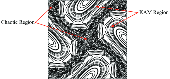
Figure 3: Two hundred iterations of the sine map (21) with $\tau=0.25$ starting from $16\times 16$ initial conditions distributed uniformly over the domain $[0,1]\times[0,1]$. The domain is periodic in both directions.

The sine flow generates a reversible map $T$ that, over one period, maps points $(x,y)$ to $T(x,y)$. The inverse of the map $T$ is given explicitly by (Gubanov and Cortelezzi, 2010)

$$T^{-1}:\begin{pmatrix}x\\ y\end{pmatrix}\mapsto\begin{pmatrix}x-\tau\sin(2\pi y)\\ y-\tau\sin\big{(}2\pi(x-\tau\sin(2\pi y))\big{)}\end{pmatrix}\mod{1}.$$ (21)

Figure 3 shows $200$ iterations of this map with $\tau=0.25$ launched from a uniform grid of initial conditions. The map $T^{-1}$ has two hyperbolic fixed points located at $(0,0)$ and $(0.5,0.5)$ whose tangle of stable and unstable manifolds creates a chaotic mixing region. In addition, the map has two elliptic fixed points located at $(0.5,0)$ and $(0,0.5)$. These elliptic fixed points are surrounded by invariant Kolmogorov–Arnold-Moser (KAM) tori with quasi-periodic motion that inhibit mixing (Arnold and Khesin, 1998).

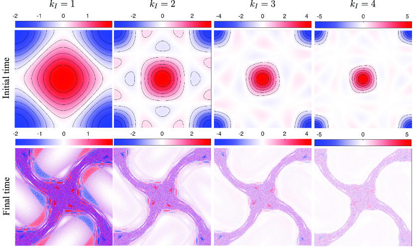
Figure 4: The optimal initial conditions $f_{\mbox{\tiny opt}}\in V_{I}$ for the sine map, with $V_{I}$ being the Fourier-based subspace defined in (13). Four optimal initial conditions with $k_{I}=1$, $2$ , $3$ and $4$ are shown in the top panel. The range of the truncated PF operator $\mathcal{P}_{p}$ is the Fourier-based subspace $V_{\nu}$ with $k_{\nu}=256$. The bottom panel shows their corresponding advected image $\mathcal{P}f_{\mbox{\tiny opt}}$ under $200$ iterations of the sine map. All figures show the entire domain $\mathcal{D}=[0,1]\times[0,1]$.

It is known that mixing is more efficient around the hyperbolic fixed points due to their tangle of stable and unstable manifolds (Aref, 1984). The KAM regions, in contrast, form islands of coherent motion that inhibit efficient mixing of passive tracers. Therefore, it is desirable to release the tracer blobs around the hyperbolic fixed points, avoiding the KAM region. Here, we examine whether the optimal initial condition given by Theorem 1 agrees with this intuitive assessment.

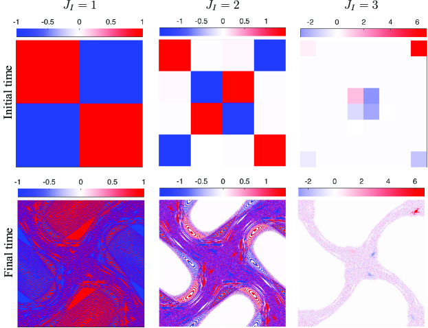
Figure 5: The optimal initial conditions $f_{\mbox{\tiny opt}}\in V_{I}$ for the sine map. Four optimal initial conditions with $J_{I}=1$, $2$ , $3$ are shown in the top panel. The bottom panel shows their corresponding advected images $\mathcal{P}f_{\mbox{\tiny opt}}$ under $200$ iterations of the sine map. The range of the truncated PF operator $\mathcal{P}_{p}$ is the Fourier-based subspace $V_{\nu}$ with $k_{\nu}=256$. All figures show the entire domain $\mathcal{D}=[0,1]\times[0,1]$.

For the finite-time analysis, we consider the flow under $200$ iterations of the sine map, i.e. we set the flow map $\varphi=T^{200}$. First, we consider the Fourier-based initial subspace $V_{I}$ defined in (13). Figure 4 shows the optimal initial conditions obtained from Theorem 1 with $k_{I}=1,2,3$ and $4$. For all parameter values $k_{I}$, the optimal initial condition consists of two prominent blobs centered at the hyperbolic fixed points $(0,0)$ and $(0.5,0.5)$. For $k_{I}=1$, only very large scales are available for the distribution of the tracer blob and therefore some intersection with the KAM region is inevitable. As the number of available wave numbers $k_{I}$ (or equivalently, available initial length scales) increases the blobs become more concentrated at the hyperbolic fixed points.

Even for $k_{I}=4$, the optimal initial condition has very small but non-zero concentration in the KAM regions. This is due to the global nature of the Fourier modes which inhibits the perfect localization around the hyperbolic fixed points. The wavelet-bases subspace (18) does not suffer from this drawback. Figure 5, for instance, shows three optimal initial conditions in this wavelet-based subspace. For $J_{I}=1$, where only the largest scales are available, intersection with the KAM region is inevitable (similar to the case of $k_{I}=1$ in figure 4). As the smaller scales become available, the optimal initial condition $f_{\mbox{\tiny opt}}$ concentrates around the hyperbolic fixed points with no concentration at the KAM regions.

The results in figures 4 and 5 are computed using the Fourier-based subspace $V_{\nu}$ with $k_{\nu}=256$. To ensure the insensitivity of the results to perturbations, we recomputed them by varying the cut-off wavenumber in the interval $250\leq k_{\nu}\leq 260$ and obtained almost identical optimal initial conditions.

5.2 Two-dimensional turbulence

As the second example, we consider a fully unsteady flow obtained from a direct numerical simulation of the two-dimensional Navier–Stokes equation,

$$\partial_{t}\mathbf{u}+\mathbf{u}\cdot\boldsymbol{\nabla}\mathbf{u}=-\boldsymbol{\nabla}p+\nu\Delta\mathbf{u}+\mathbf{F},\quad\boldsymbol{\nabla}\cdot\mathbf{u}=0,$$ (22)

with the dimensionless viscosity $\nu=10^{-5}$ and a band-limited stochastic forcing $\mathbf{F}$. The flow domain is the box $\mathcal{D}=[0,2\pi]\times[0,2\pi]$ with periodic boundary conditions. A standard pseudo-spectral code with 2/3 dealiasing was used to numerically solve the Navier–Stokes equations (see Section 6.2 of Farazmand and Haller (2016) for further computational details).

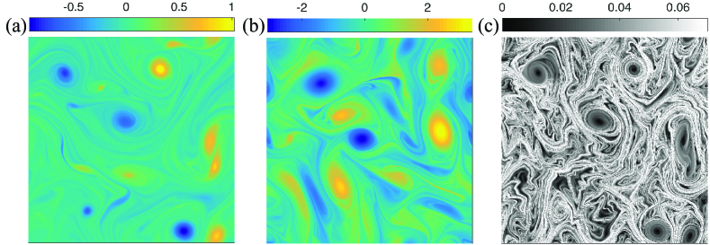
Figure 6: (a) The vorticity field at the initial time $t_{0}$. (b) The vorticity field at the final time $t_{0}+T$. (c) The forward-time FTLE field corresponding to the time interval $[t_{0},t_{0}+T]$. Here, $T$ is $100$ time units.

Starting from a random-phase initial condition, we numerically integrate the Navier–Stokes equation. After $1000$ time units the flow has reached a statistically steady turbulent state with Reynolds number $4.1\times 10^{3}$. We set this time as the initial time $t_{0}$ for the mixing analysis. The final time instance is set to $t_{0}+T$ with $T=100$. Figures 6(a,b) show the vorticity fields at these initial and final times.

As is typical of two-dimensional turbulence, the flow contains several coherent vortices that exhibit minimal material deformation over the time interval $[t_{0},t_{0}+T]$ (McWilliams, 1984). These coherent vortices are signaled by the islands of small finite-time Lyapunov exponent (FTLE) shown in figure 6(c). The FTLE field is computed as $\log[\lambda(\mathbf{x})]/(2T)$ for all $\mathbf{x}\in\mathcal{D}$, with $\lambda(\mathbf{x})$ being the largest eigenvalue of the Cauchy–Green strain tensor $[\mathrm{d}\varphi(\mathbf{x})]^{\top}\mathrm{d}\varphi(\mathbf{x})$, and $\mathrm{d}\varphi$ denoting the Jacobian of the flow map (Voth et al., 2002). Outside the coherent vortices the flow is mostly chaotic, dominated by the stretching and folding of material lines.

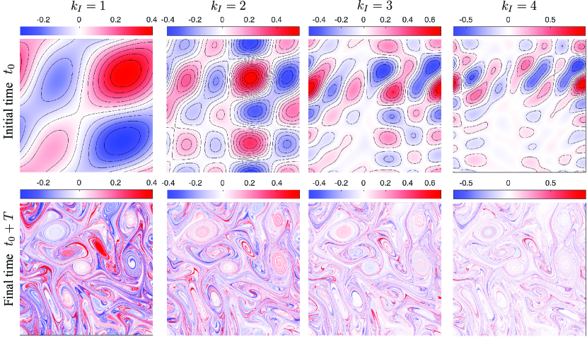
Figure 7: Optimal initial tracers $f_{\mbox{\tiny opt}}\in V_{I}$ (upper panel) in the turbulent flow with $k_{I}=1,2,3$ and $4$. Their corresponding advected images $\mathcal{P}f_{\mbox{\tiny opt}}$ at the final time $t_{0}+T$ are shown in the lower panel. In all four cases shown here, the mixed wavenumber is $k_{\nu}=256$ (see equation (14)). All panels show the entire domain $\mathcal{D}=[0,2\pi]\times[0,2\pi]$.

Next we compute the optimal initial conditions $f_{\mbox{\tiny opt}}$. Unlike the sine map, the preimages $\varphi^{-1}(\mathbf{x}_{0})$ are not explicitly known here. We numerically evaluate the preimages by integrating the ODE (2) backwards in time from the final time $t_{0}+T$ to the initial time $t_{0}$, for each initial condition $\mathbf{x}_{0}\in\mathcal{G}$. This numerical integration is carried out by the fifth-order Runge-Kutta scheme of Dormand and Prince (1980). Since the velocity field $\mathbf{u}$ is stored on a discrete spatiotemporal grid, it needs to be interpolated for the particle advection. Here, we use cubic splines for the spatial interpolation of the velocity field together with a linear interpolation in time.

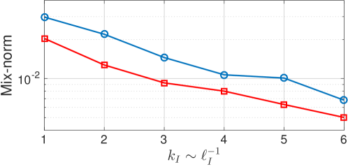
Figure 8: Red line (squares): The mix-norm $\|\mathcal{P}f_{\mbox{\tiny opt}}\|_{H^{-1}}$ for the optimal initial concentrations $f_{\mbox{\tiny opt}}\in V_{I}$. The optimal initial conditions for $k_{I}=1$, $2$, $3$ and $4$ are shown in figure 7. Blue line (circles): The mix-norm $\|\mathcal{P}f\|_{H^{-1}}$ for the initial concentrations $f(x,y)=\cos(k_{I}x)\cos(k_{I}y)/\pi$.

Figure 7 shows the optimal initial tracer patterns $f_{\mbox{\tiny opt}}$ for $k_{I}=1,2,3$ and $4$, which belong to the corresponding Fourier-based subspaces $V_{I}$ as defined in equation (13). As opposed to the simple model considered in Section 5.1, the optimal tracer patterns here have fairly complicated structures. This is to be expected as the turbulent flow itself has a complex spatiotemporal structure.

Ideally, the tracer should concentrate outside the coherent vortices to achieve better mixing. Similar to the sine flow, for $k_{I}=1$, where only the very large scales are available for the release of the tracer, there is some inevitable overlap between the coherent vortices and the tracer. This results in the visibly unmixed blobs in the advected tracers $\mathcal{P}f_{\mbox{\tiny opt}}$ shown in the lower panel of figure 7. Theorem 1, however, guarantees that the optimal initial condition $f_{\mbox{\tiny opt}}$ is such that the unmixed blobs are minimal. As smaller scales become available ($k_{I}>1$), the intersection of the high initial tracer concentration and the coherent vortices becomes smaller, leading to a more homogeneous mixture after advection to the final time $t_{0}+T$.

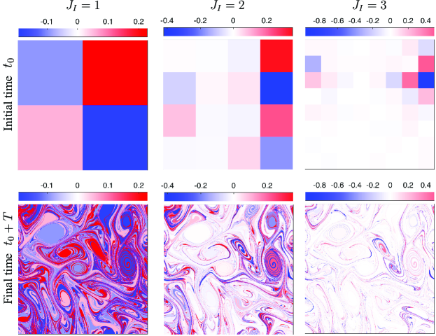
Figure 9: Optimal initial tracers $f_{\mbox{\tiny opt}}\in V_{I}$ (upper panel) in the turbulent flow with $J_{I}=1,2$ and $3$. Their corresponding advected images $\mathcal{P}f_{\mbox{\tiny opt}}$ at the final time $t_{0}+T$ are shown in the lower panel. In all four cases shown here, the mixed wavenumber is $k_{\nu}=256$ (see equation (14)). All panels show the entire domain $\mathcal{D}=[0,2\pi]\times[0,2\pi]$.

To quantify the mixture qualities, we compute the mix-norm of the advected tracers proposed by Shaw et al. (2007). This mix-norm is the Sobolev $H^{-1}$ norm,

$$\|\rho\|_{H^{-1}}=\sqrt{\sum_{\mathbf{k}\neq\mathbf{0}}|\widehat{\rho}(\mathbf{k})|^{2}/|\mathbf{k}|^{2}},$$ (23)

where the hat sign denotes the Fourier transform. Mathew et al. (2007) proposed the alternative Sobolev norm $H^{-1/2}$ for quantifying the mixture quality. The motivation for using such Sobolev norms is that the density of homogeneous mixtures are concentrated at ever smaller scales or equivalently larger wave numbers $|\mathbf{k}|$. As a result, more homogeneous mixtures have smaller mix-norms.

The mix-norm $\|\mathcal{P}f_{\mbox{\tiny opt}}\|_{H^{-1}}$ is shown in figure 8 for the optimal initial conditions $f_{\mbox{\tiny opt}}\in V_{I}$ with $1\leq k_{I}\leq 6$. As $k_{I}$ increases, more homogeneous mixtures are obtained, as is also visible in figure 7. For comparison, we also show the mix-norm $\|\mathcal{P}f\|_{H^{-1}}$ for the non-optimal initial conditions $f(x,y)=\cos(k_{I}x)\cos(k_{I}y)/\pi\in V_{I}$. The non-optimal initial conditions result into a larger mix-norm, showing that they do not mix as well as the optimal initial conditions $f_{\mbox{\tiny opt}}$ do. Figure 5 shows the optimal initial conditions found in the wavelet-based subspace (18). Their mix-norms exhibit a similar behavior as the one shown in figure 8.

6 Concluding remarks

The design of mixing devices has primarily been concerned with the stirring protocols that enhance mixing. The optimality of these protocols are limited by design constraints and fundamental physics (Lin et al., 2011). On the other hand, for a given stirring protocol, the final mixture quality also depends on the initial configuration of the tracer. The optimal initial condition for the release of the tracer has received far less attention.

Here, we proposed a rigorous framework for determining the optimal initial tracer configuration to achieve maximal mixing under finite-time passive advection. We showed that, under reasonable assumptions, the problem reduces to a finite-dimensional optimization problem. The optimal initial condition then coincides with a singular vector of a truncated Perron–Frobenius (PF) operator. This truncation is not an approximation of the infinite-dimensional PF operator; it rather follows naturally from our simplifying assumption that the tracer blobs smaller than a prescribed critical length scale $\ell_{\nu}$ are completely mixed.

We discussed two numerical implementations of the optimization problem using Fourier modes and Haar wavelets. While the Fourier modes are convenient for the spatially periodic flows considered here, the wavelets are more suitable for handing more complicated geometries and boundary conditions. Wavelets also allow for optimal initial conditions that are local in both space and scale. The space localization is crucial in many applications where the tracer can only be released into a subset of the flow domain duo to geometric constraints.

We restricted our attention here to ideal passive tracers. Future work will expand the framework to account for diffusion and the presence of sinks and sources. Diffusion, in particular, dictates a dissipative length scale $\ell_{\nu}$ for mixed blobs which, in the absence of diffusion, was prescribed here in an ad-hoc manner.

Acknowledgments: I would like to thank Daniel Karrasch for pointing out the correct terminology in Definition 4 and bringing a number of relevant references to my attention. I am also grateful to Charles Doering, Gary Froyland, George Haller and Christopher Miles for their comments on this manuscript.

References

- Aref (1984) H. Aref. Stirring by chaotic advection. J. Fluid Mech., 143:1–21, 1984.
- Arnold and Khesin (1998) V. I. Arnold and B. A. Khesin. Topological methods in hydrodynamics, volume 125. Springer, 1998.
- Daubechies (1992) I. Daubechies. Ten Lectures on Wavelets, volume 61. SIAM, 1992.
- Dellnitz and Junge (1999) M. Dellnitz and O. Junge. On the approximation of complicated dynamical behavior. SIAM Journal on Numerical Analysis, 36(2):491–515, 1999.
- Dellnitz et al. (2001) M. Dellnitz, G. Froyland, and O. Junge. The algorithms behind GAIO–set oriented numerical methods for dynamical systems. In Ergodic theory, analysis, and efficient simulation of dynamical systems, pages 145–174. Springer, 2001.
- Dormand and Prince (1980) J. R. Dormand and P. J. Prince. A family of embedded Runge–Kutta formulae. J. Comp. App. Math., 6(1):19 – 26, 1980.
- Farazmand and Haller (2016) M. Farazmand and G. Haller. Polar rotation angle identifies elliptic islands in unsteady dynamical systems. Physica D, 315:1–12, 2016.
- Farazmand et al. (2011) M. Farazmand, N. K.-R. Kevlahan, and B. Protas. Controlling the dual cascade of two-dimensional turbulence. J. Fluid Mech., 668:202–222, 2011.
- Farge et al. (1999) M. Farge, K. Schneider, and N. Kevlahan. Non-gaussianity and coherent vortex simulation for two-dimensional turbulence using an adaptive orthogonal wavelet basis. Phys. Fluids, 11(8):2187–2201, 1999.
- Foures et al. (2014) D. P. G. Foures, C. P. Caulfield, and P. J. Schmid. Optimal mixing in two-dimensional plane Poiseuille flow at finite Péclet number. J. Fluid Mech., 748:241–277, 2014.
- Froyland (2013) G. Froyland. An analytic framework for identifying finite-time coherent sets in time-dependent dynamical systems. Physica D, 250:1–19, 2013.
- Froyland and Padberg (2009) G. Froyland and K. Padberg. Almost-invariant sets and invariant manifolds—connecting probabilistic and geometric descriptions of coherent structures in flows. Physica D, 238(16):1507–1523, 2009.
- Froyland and Padberg-Gehle (2014) G. Froyland and K. Padberg-Gehle. Almost-invariant and finite-time coherent sets: directionality, duration, and diffusion. In Ergodic Theory, Open Dynamics, and Coherent Structures, pages 171–216. Springer, 2014.
- Froyland et al. (2007) G. Froyland, K. Padberg, M. H. England, and A. M. Treguier. Detection of coherent oceanic structures via transfer operators. Phys. Rev. Lett., 98(22):224503, 2007.
- Froyland et al. (2010) G. Froyland, N. Santitissadeekorn, and A. Monahan. Transport in time-dependent dynamical systems: Finite-time coherent sets. Chaos, 20(4):043116, 2010.
- Gouillart et al. (2006) E. Gouillart, J.-L. Thiffeault, and M. D. Finn. Topological mixing with ghost rods. Phys. Rev. E, 73(3):036311, 2006.
- Gubanov and Cortelezzi (2009) O. Gubanov and L. Cortelezzi. Sensitivity of mixing optimization to the geometry of the initial scalar field. In L. Cortelezzi and I. Mezić, editors, Analysis and Control of Mixing with an Application to Micro and Macro Flow Processes, pages 369–405. Springer, Vienna, 2009.
- Gubanov and Cortelezzi (2010) O. Gubanov and L. Cortelezzi. Towards the design of an optimal mixer. J. Fluid Mech., 651:27–53, 2010.
- Hobbs and Muzzio (1997) D. M. Hobbs and F. J. Muzzio. Effects of injection location, flow ratio and geometry on Kenics mixer performance. AIChE, 43(12):3121–3132, 1997.
- Iyer et al. (2014) G. Iyer, A. Kiselev, and X. Xu. Lower bounds on the mix norm of passive scalars advected by incompressible enstrophy-constrained flows. Nonlinearity, 27(5):973, 2014.
- Lasota and Mackey (1994) A. Lasota and M. C. Mackey. Chaos, fractals, and noise: Stochastic aspects of dynamics, volume 97 of Applied Mathematical Sciences. Springer, second edition, 1994. New York.
- Lin et al. (2011) Z. Lin, J.-L. Thiffeault, and C. R. Doering. Optimal stirring strategies for passive scalar mixing. J. Fluid Mech, 675:465–476, 2011.
- Liu et al. (1994) M. Liu, F. J. Muzzio, and R. L. Peskin. Quantification of mixing in aperiodic chaotic flows. Chaos, Solitons & Fractals, 4(6):869–893, 1994.
- Lunasin et al. (2012) E. Lunasin, Z. Lin, A. Novikov, A. Mazzucato, and C. R. Doering. Optimal mixing and optimal stirring for fixed energy, fixed power, or fixed palenstrophy flows. J. Math. Phys., 53(11):115611, 2012.
- Mathew et al. (2007) G. Mathew, I. Mezić, S. Grivopoulos, U. Vaidya, and L. Petzold. Optimal control of mixing in Stokes fluid flows. J. Fluid Mech, 580:261–281, 2007.
- McWilliams (1984) J. C. McWilliams. The emergence of isolated coherent vortices in turbulent flow. J. Fluid Mech., 146:21–43, 1984.
- Okabe et al. (2008) T. Okabe, B. Eckhardt, J.-L. Thiffeault, and C. R. Doering. Mixing effectiveness depends on the source–sink structure: simulation results. Journal of Statistical Mechanics: Theory and Experiment, 2008(07):P07018, 2008.
- Pierrehumbert (1994) R. T. Pierrehumbert. Tracer microstructure in the large-eddy dominated regime. Chaos, Solitons & Fractals, 4(6):1091–1110, 1994.
- Press et al. (2007) W. H. Press, S. A. Teukolsky, W. T. Vetterling, and B. P. Flannery. Numerical recipes: The art of scientific computing. Cambridge University Press, third edition, 2007.
- Protas (2008) B. Protas. Adjoint-based optimization of PDE systems with alternative gradients. J. Comp. Physics, 227(13):6490 – 6510, 2008.
- Santitissadeekorn et al. (2010) N. Santitissadeekorn, G. Froyland, and A. Monahan. Optimally coherent sets in geophysical flows: A transfer-operator approach to delimiting the stratospheric polar vortex. Physical Review E, 82(5):056311, 2010.
- Seis (2013) C. Seis. Maximal mixing by incompressible fluid flows. Nonlinearity, 26(12):3279, 2013.
- Shaw et al. (2007) T. A. Shaw, J.-L. Thiffeault, and C. R. Doering. Stirring up trouble: Multi-scale mixing measures for steady scalar sources. Physica D, 231(2):143 – 164, 2007.
- Singh et al. (2008) M. K. Singh, P. D. Anderson, M. F. M. Speetjens, and H. E. H. Meijer. Optimizing the rotated arc mixer. AIChE, 54(11):2809–2822, 2008.
- Stewart (1998) G. W. Stewart. Matrix Algorithms. SIAM, 1998.
- Stroock et al. (2002) A. D. Stroock, S. K. W. Dertinger, A. Ajdari, I. Mezić, H. A. Stone, and G. M. Whitesides. Chaotic mixer for microchannels. Science, 295(5555):647–651, 2002.