Strengths and weaknesses of weak-strong cluster problems:
A detailed overview of state-of-the-art classical heuristics vs quantum approaches

Abstract

To date, a conclusive detection of quantum speedup remains elusive. Recently, a team by Google Inc. [V. S. Denchev et al., Phys. Rev. X 6, 031015 (2016)] proposed a weak-strong cluster model tailored to have tall and narrow energy barriers separating local minima, with the aim to highlight the value of finite-range tunneling. More precisely, results from quantum Monte Carlo simulations, as well as the D-Wave 2X quantum annealer scale considerably better than state-of-the-art simulated annealing simulations. Moreover, the D-Wave 2X quantum annealer is $\sim 10^{8}$ times faster than simulated annealing on conventional computer hardware for problems with approximately $10^{3}$ variables. Here, an overview of different sequential, nontailored, as well as specialized tailored algorithms on the Google instances is given. We show that the quantum speedup is limited to sequential approaches and study the typical complexity of the benchmark problems using insights from the study of spin glasses.

Section I Introduction

Adiabatic quantum optimization (QA) Nielsen and Chuang (2000); Nishimori (2001); Finnila et al. (1994); Kadowaki and Nishimori (1998); Brooke et al. (1999); Farhi et al. (2000); Roland and Cerf (2002); Santoro et al. (2002); Das and Chakrabarti (2005); Santoro and Tosatti (2006); Lidar (2008); Das and Chakrabarti (2008); Morita and Nishimori (2008); Mukherjee and Chakrabarti (2015), the quantum version of classical simulated annealing (SA) Kirkpatrick et al. (1983), has caused considerable controversy and interest since the introduction of the D-Wave Inc. com (a) quantum annealing machines Johnson et al. (2011). Although there is increasing evidence that quantum effects do play a role in the optimization process of these machines, there is still no consensus as to if the machine is able to outperform classical optimization heuristics on silicon-based computer hardware. Multiple teams Dickson et al. (2013); Pudenz et al. (2014); Smith and Smolin (2013); Boixo et al. (2013); Rønnow et al. (2014a); Katzgraber et al. (2014); Lanting et al. (2014); Santra et al. (2014); Shin et al. (2014); Boixo et al. (2014a); Albash et al. (2015a, b); Katzgraber et al. (2015); Martin-Mayor and Hen (2015); Pudenz et al. (2015); Hen et al. (2015); Venturelli et al. (2015); Vinci et al. (2015); Zhu et al. (2016) have scrutinized this first commercially available programmable analog quantum optimizer [the current version being the D-Wave 2X (DW2X) with up to $1152$ quantum bits wired on a chimera topology Bunyk et al. (2014)] and tried to understand its advantages and disadvantages over classical technologies, as well as improve its performance via, e.g., quantum error correction Lidar and Brun (2013); Pudenz et al. (2015); Vinci et al. (2015) (at the price of having too few logical qubits for a scaling analysis) or fine-tuning of the device Perdomo-Ortiz et al. (2015a, b).

In an effort to determine the thermodynamic (large number of qubits $n$) scaling advantage of a quantum annealer over conventional algorithms, it is of importance to use the largest possible number of qubits on any device. As such, embedded problems (that might require an overhead due to the embedding) are sub-optimal for scaling analyses. Native problems, such as spin-glass-like systems Binder and Young (1986); Stein and Newman (2013) that use all qubits of the system, are thus optimal to tickle out any putative quantum advantage from quantum annealing machines. Unfortunately, results have been inconclusive so far Rønnow et al. (2014a) and there is strong evidence that random spin-glass problems are not well suited for benchmarking purposes Katzgraber et al. (2014, 2015). Thus, efforts have shifted to tailored problems, such as carefully-crafted spin-glass instances Katzgraber et al. (2015); Zhu et al. (2016) that are robust to the intrinsic noise of analog machines. In particular, Ref. Katzgraber et al. (2015) suggested a slight quantum advantage over classical simulated annealing Isakov et al. (2015, 2014) using the $512$-qubit D-Wave 2 quantum annealer com (b). However, no scaling analysis was performed because systems of approximately $n\sim 500$ qubits are just at the brink of the scaling regime.

Despite all these efforts, a “killer” application or problem domain has yet to be found, where quantum annealing outperforms notably classical simulational approaches. In particular, given that many well-known optimization problems from the traveling salesman problem to constraint-satisfaction and vertex cover problems can be mapped onto Ising spin-glass-like Hamiltonians Lucas (2014), there is great interest from both science and industry to find efficient optimization approaches to tackle spin-glass-like Hamiltonians – the main forte of the DW2X  device. Most recently, however, a team by Google Inc. Denchev et al. (2016) showed for carefully-crafted problems that quantum annealing on the DW2X  can outperform classical simulated annealing by approximately eight orders of magnitude. Furthermore, the scaling of quantum approaches (both on the DW2X  and using quantum Monte Carlo Suzuki (1993)) is considerably better than for classical simulated annealing. We believe this is the first notable “success story” for quantum annealing. However, numerical comparisons were performed against one of the commonly-known least-efficient optimization methods, namely simulated annealing. While this seems to be a fair comparison because both QA and SA are sequential optimization methods where a control parameter (quantum fluctuations in the former and thermal fluctuations in the latter) is decreased monotonically until reaching a target value, it is unclear if this favorable scaling will persist for state-of-the art optimization methods (see, for example, Refs. Hartmann and Rieger (2001); Elf et al. (2001); Hartmann and Rieger (2004); Zhu et al. (2015) for some examples). We do emphasize, however, that the Google Inc. studies Boixo et al. (2014b); Denchev et al. (2016); Boixo et al. (2016) shed, for the first time, some light on the structure of problems where quantum annealing might excel. In particular, by carefully crafting weak-strong cluster problems (see Sec. III for details), they can show that there is a sign of finite-range quantum tunneling, at least within the basic building blocks of the DW2X  device, known as a $\text{K}_{4,4}$ cell Denchev et al. (2016).

In this work, we complement the study of Ref. Denchev et al. (2016): first, we expand the notion of “limited quantum speedup” Rønnow et al. (2014a) to take into account different classes of algorithms (see Sec. II) and thus attempt to present a fair assessment of any sequential quantum annealer. In particular, we introduce the notion of “limited sequential quantum speedup” which refers to speedup with respect to any algorithm that optimizes sequentially such as, for example, simulated annealing. Furthermore, we distinguish two types of state-of-the-art optimization methods: “tailored” and “nontailored” algorithms. Tailored algorithms exploit the structure of the studied optimization problem; we thus feel this might pose an unfair advantage. Nontailored algorithms are generic, and thus present the state of the art when studying a wide variety of optimization problems. Our results show that sequential quantum approaches (DW2X  quantum annealer and quantum Monte Carlo) clearly outperform any other currently-available sequential methods, but fall short of outperforming nontailored (as well as tailored) algorithms. We thus herewith raise the bar for any quantum optimization approach. Second, we illustrate with a simple two-energy level model with noise, how a suboptimal annealing time for small problem sizes can lead to a change in slope of the scaling analysis, as observed in Ref. Denchev et al. (2016) for the DW2X  machine. Finally, we study the energy landscape of the instances and show that the spin-glass backbone of the weak-strong cluster network dominates and thus might negatively impact the scaling of this class of problem for future larger chips and/or system sizes.

The paper is structured as follows. In Sec. II, we introduce a classification for the concept of “quantum speedup”, in order to better assess the comparison between classical and quantum devices. In Sec. III, we briefly describe the weak-strong cluster model, followed by a summary of our results in Sec. IV. Concluding remarks are summarized in Sec. V. All the algorithms used in this study are outlined in the Appendix.

Section II Limited quantum speedup redefined

Given the intrinsic differences between classical and quantum heuristics, it is impossible to define a simple recipe to quantify “quantum speedup.” In Ref. Rønnow et al. (2014b), the authors discuss in detail the meaning of quantum speedup, defining different “classes” of speedup to better quantify any putative speedup of a quantum device com (c). More precisely, they classify quantum heuristics in four different classes, ranging from the class with the strongest proof of quantum enhancement to the class with the weakest proof, as follows:

Provable quantum speedupi. It is rigorously proven that no classical algorithm can scale better than a given quantum algorithm. For example, the Grover algorithm (assuming an oracle) Grover (1997) belongs to this class.

Strong quantum speedup. Originally defined in Ref. Papageorgiou and Traub (2013), strong quantum speedup refers to a comparison with the best classical algorithm, regardless if the algorithm exists or not. Note, however, that the “best classical algorithm” might not be known or there might be no consensus as to what the best classical algorithm is. For example, the well-known Shor quantum algorithm for the factorization of prime numbers Shor (1997) belongs to this class.

Potential quantum speedup. Refers to speedup when comparing to a specific classical algorithm or a set of classical algorithms. In this case, any potential quantum speedup might be short lived if a better classical algorithm is developed. An example is the simulation of the time evolution of a quantum system, where the propagation of the wave function on a quantum computer would be exponentially faster than the direct integration of the Schrödinger equation.

Limited quantum speedup. Speedup obtained by comparing the algorithmic approach used in a quantum computer to the closer classical counterpart. Usually, quantum Monte Carlo (QMC) is used for the comparison with adiabatic quantum optimization Santoro et al. (2002); Boixo et al. (2014a); Rønnow et al. (2014b).

The introduction of the aforementioned categories has helped enormously in ensuring that there are no misunderstandings when referring to quantum speedup. Indeed, these general categories have the advantage that they cover a broad class of quantum computing paradigms. However, given that, at the moment, analog quantum annealing machines dominate this field of research, it might be of importance to introduce definitions for quantum speedup tailored towards these machines. Therefore, to be able to perform a fair assessment of speedup for quantum annealing machines, we introduce the following definitions that complement the notion of “limited quantum speedup:”

Limited sequential quantum speedup. Speedup obtained by comparing a quantum annealing algorithm or machine to any sequential algorithm [e.g., simulated annealing (SA) Kirkpatrick et al. (1983), or population annealing (PA) Monte Carlo Hukushima and Iba (2003); Machta (2010); Wang et al. (2015a, b)] where a control parameter is monotonously tuned until a certain threshold is reached (e.g., the temperature in SA or the transverse field in QA). While sequential methods might not necessarily be the best classical optimization algorithm, they are the classical counterpart to quantum annealing.

Limited nontailored quantum speedup. Speedup obtained by comparing a quantum annealing algorithm or machine to the best-known generic classical optimization algorithm that is not tailored to a particular problem and does not exploit particular knowledge of the problem to be optimized [e.g., isoenergetic cluster optimizers (ICM) Zhu et al. (2015), or the groups method Zintchenko et al. (2015)].

Limited tailored quantum speedup. Speedup obtained by comparing a quantum annealing algorithm or machine to the best-known tailored classical optimization algorithm that explicitly exploits the structure of the problem to be optimized and will perform in a sub-optimal fashion (if work at all) on any other type of optimization problem [examples are hybrid cluster moves (HCM) Venturelli et al. (2015) or the Hamze–de-Freitas–Selby (HFS) algorithm Hamze and de Freitas (2004); Selby (2014)].

Given the sequential nature of transverse-field quantum annealing, limited sequential quantum speedup is naturally the fairest comparison to classical counterparts. However, this might not be of much use if classical sequential algorithms are slow compared to other classical optimization methods. A comparison to tailored algorithms is slightly unfair, because the structure of the problem is being exploited, i.e., the developer of the algorithm knows a priori how to design the algorithm to outperform quantum annealing. We do emphasize that it might be misleading to compare limited tailored quantum speedup to potential quantum speedup because the classical algorithm is specifically designed to outperform the quantum counterpart. However, comparing to nontailored classical algorithms is similar to potential quantum speedup. The classical approach is generic and widely applicable and makes no assumptions about the studied problem. In addition, it should be the currently fastest optimizer available com (d).

Finally quantum annealing with a transverse field is the simplest possible quantum-enhanced algorithm. Going beyond more complex driving Hamiltonians (e.g., non-stoquastic Matsuda et al. (2009), different initial states Crosson et al. (2014), the insertion of Hamiltonians during the annealing Perdomo-Ortiz et al. (2011), or schedule randomization com (e)), one could easily imagine implementing far more complex quantum algorithms that exploit the current advantages of classical methods. For example, quantum cluster updates can be implemented by suitably coupling two systems with the same target Hamiltonian together, or quantum population annealing by running multiple quantum chips in parallel and culling the least fit copies of the target Hamiltonian. Once the field of quantum optimization has reached this stage of development, the aforementioned defined categories will require adjustments to take into account these advances.

Section III Weak-Strong cluster model

The weak-strong cluster network is a tailored model designed to exploit quantum tunneling in quantum optimizers and, therefore, to demonstrate how finite-range tunneling can provide a computational advantage over classical heuristics Denchev et al. (2016). The model is composed by highly-connected and ferromagnetically coupled clusters ($J=1$) (corresponding to the unit cells of the chimera graph Bunyk et al. (2014)) that interact with each other (see Fig. 1). These clusters can be divided in two classes: “strong” clusters, which form the spin-glass bulk of the model, and “weak” clusters, which are ferromagnetically coupled to strong clusters. To complete the model, an external field is applied to all the spins of the system: a “strong” negative external field $h_{1}=-1$ to those spins belonging to strong clusters and a “weak” positive external field $h_{2}=-\lambda h_{1}=0.44<1/2$ to those spins belonging to weak clusters. The ground state of the system is therefore the configuration with all spins of both weak and strong clusters pointing along the direction of the strong local field. Individual weak-strong clusters are coupled by a spin-glass backbone where the interactions between the clusters can take values $\{\pm 1\}$. Note that the interactions between weak-strong clusters only occur between sites in the strong cluster. See Figure 3 of Ref. Denchev et al. (2016) for the actual graphs simulated on the DW2X  quantum annealer. The peculiarity of the weak-strong cluster model is that there exists a bifurcation point during both the classical and quantum annealing where the system is forced to follow a “wrong” path leading to a local minimum, namely the configuration with spins in weak clusters pointing toward the weak external field. However, quantum annealers, unlike classical annealers, can tunnel earlier to the “correct” path and, eventually, reach the true ground state of the system.

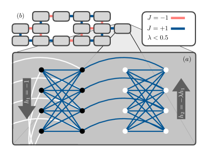
Figure 1: Sketch of the weak-strong clusters and networks. (a) Structure of a weak-strong cluster. Two $\text{K}_{4,4}$ cells of the chimera lattice are connected ferromagnetically (blue lines, $J=1$), as well as all spins within each $\text{K}_{4,4}$ cell. Black dots correspond to qubits in the strong cluster with a biasing magnetic field $h_{1}=-1$. The white dots represent the weak cluster, where each site is coupled to a weaker field $h_{2}=-\lambda h_{1}$ with $\lambda=0.44<0.5$ in the opposite direction. The white lines represent the connections from the strong cluster to neighboring strong clusters of a weak-strong pair. (b) Weak-strong cluster network: each rectangle represents a weak-strong cluster. The different weak-strong clusters are connected via a spin-glass backbone where the interactions can take values $J_{\bar{x}\bar{x}^{\prime}}=\pm 1$. Here, red lines represent $J=-1$. Note that the connections between clusters only occur between the strong clusters.

The Hamiltonian describing the weak-strong cluster model is composed of four main terms: the Hamiltonian describing the strong (weak) clusters $\mathcal{H}_{1}$ ($\mathcal{H}_{2}$) and the Hamiltonians describing either the interaction between strong clusters $\mathcal{H}_{1,1}$ or the interaction between strong and weak clusters $\mathcal{H}_{1,2}$ (see Ref. Denchev et al. (2016) for details). Each pair of weak-strong cluster can be seen as a single functional cluster [i.e. a single gray box in Figure 1(b)], labeled by a two-dimensional spatial position $\bar{x}$. Strong clusters belonging to two different functional cluster are then linked with random couplings ($J_{\bar{x}\bar{x}^{\prime}}=\pm 1$) following a pre-determined backbone $\mathcal{B}$. Note that the weak clusters only couple to the strong cluster within a given weak-strong cluster. More precisely, for $\ell=\{1,\,2\}$ the aforementioned Hamiltonians have the form

$${\mathcal{H}}^{\bar{x}}_{\ell}=-J\sum_{i,j\in{\mathcal{V}_{\bar{x}}}}\sigma_{\ell,i}^{z}\sigma_{\ell,j}^{z}-\sum_{i\in{\mathcal{V}}_{\bar{x}}}h_{\ell}\sigma_{\ell,i}^{z}$$ (1)

and

$${\mathcal{H}}_{1,1}^{\bar{x},\bar{x}^{\prime}} =-\sum_{j\in{{\mathcal{V}}}_{\bar{x},\bar{x}^{\prime}}}J_{\bar{x},\bar{x}^{\prime}}\sigma_{1,j}^{z}\sigma_{1,j}^{z},$$ (2a)

$${\mathcal{H}}_{1,2}^{\bar{x}} =-J\sum_{j\in\tilde{{\mathcal{V}}}_{\bar{x}}}\sigma_{1,j}^{z}\sigma_{2,j}^{z},$$ (2b)

where $\mathcal{V}_{\bar{x}}$ represents the eight vertices in one $\text{K}_{4,4}$ unit cell of the chimera graph for the functional cluster in the position $\bar{x}$. The set ${\mathcal{V}}_{\bar{x},\bar{x}^{\prime}}$ represents the vertices on the left-hand side which couple two adjacent strong clusters while the set $\tilde{{\mathcal{V}}}_{\bar{x}}$ represents the vertices of the right-hand side of the strong and weak clusters that are linked by a ferromagnetic interaction $J=1$. Putting together Eqs. (1) and (2), the final problem Hamiltonian for the weak-strong cluster model assumes the form:

$$\mathcal{H}=\sum_{\bar{x}\in\mathcal{B}}\Big{[}\mathcal{H}^{\bar{x}}_{1}+\mathcal{H}^{\bar{x}}_{2}+\mathcal{H}^{\bar{x}}_{1,2}\Big{]}+\sum_{(\bar{x},\bar{x}^{\prime})\in\mathcal{B}}\mathcal{H}_{1,1}^{\bar{x},\bar{x}^{\prime}},$$ (3)

with $(\bar{x},\bar{x}^{\prime})$ indicating two functional clusters which are adjacent in the given backbone $\mathcal{B}$. Because of imperfections in the DW2X  device, the embedding of the weak-strong cluster network in the chimera topology is nontrivial. However, systems of up to $n=945$ qubits have been studied.

The main result of Ref. Denchev et al. (2016) is to show, either experimentally (by using the DW2X  quantum optimizer) or numerically (by using quantum Monte Carlo simulations), that quantum co-tunneling effects play a fundamental role in adiabatic optimization. Note that quantum Monte Carlo is the closest classical algorithm to quantum annealing on the DW2X. The results of Ref. Denchev et al. (2016) on the DW2X  chip are approximately $10^{8}$ times faster than simulated annealing Kirkpatrick et al. (1983) and considerably faster than quantum Monte Carlo despite both the DW2X  quantum annealer and quantum Monte Carlo having a similar scaling (similar slope of the curves in Fig. 4 of Ref. Denchev et al. (2016) for quantum Monte Carlo and the DW2X). While this, indeed, represents the first solid evidence that the DW2X  machine might have capabilities that classical optimization approaches do not possess, it is important to perform a comprehensive comparison to a wide variety of state-of-the-art optimization methods. Within the categories defined in Sec. II, the results of Ref. Denchev et al. (2016) for the DW2X  clearly outperform any sequential optimization methods, however, fall short of outperforming tailored and nontailored optimization methods. We feel, however, that knowingly exploiting the structure of a problem does not amount to a fair comparison. However, our results shown below clearly suggest that generic optimization methods still outperform the DW2X. One might thus question the importance of the results of Ref. Denchev et al. (2016). We emphasize that this is the first study that undoubtedly shows that the DW2X  machine has finite-range tunneling and gives clear hints towards the class of problems where analog quantum annealing machines might excel.

In addition to showing here that a variety of either “tailored” to the weak-strong cluster structure or more “generic” classical heuristics can achieve similar performances of the DW2X  chip, we also study the energy landscape of the weak-strong cluster networks. The latter provides valuable insights about the limitations of finite-range tunneling for this class of problems. Our analysis suggests that the scaling advantage of finite-range cotunneling over sequential algorithms could be lost for instances with problem sizes beyond the ones considered in Ref. Denchev et al. (2016).

In the next section we further discuss the performance of DW2X  compared to tailored and nontailored classical heuristics in detail.

Section IV Results

In this section, we present our main results. In the first part, we compare the performance of the DW2X  device against general (nontailored) and tailored classical algorithms. The description of the used algorithms is in the Appendix. In the second part, we analyze in depth the scaling behavior of the DW2X  device by varying the number of used qubits. The aim is to better understand the role of nonoptimal annealing times for a noisy analog device to the asymptotic scaling of the computational time. Finally, we study the energy landscape, as proposed in Ref. Katzgraber et al. (2015), and show that for increasing problem size the spin-glass backbone of the weak-strong cluster network dominates and the advantages of finite-range tunneling diminish for increasing system sizes.

IV.1 Analysis of the computational scaling

In order to compare heuristics which are fundamentally different from each other, it is necessary to define a metric which is not only fair, but that gives a quantitative measure of the speedup. In this work, and to compare on equal footing with the results in Ref. Denchev et al. (2016), we follow the time-to-solution metric introduced in Refs. Boixo et al. (2014a); Rønnow et al. (2014b). This metric is defined as the time to find the ground state with $99\%$ of confidence after a given number of repeated runs, namely,

$$T_{\text{tts}}=T_{\text{ann}}R=T_{\text{ann}}\frac{\log_{10}(1-0.99)}{\log_{10}[1-p_{\text{succ}}(T_{\text{ann}})]},$$ (4)

where $T_{\text{ann}}$ is the annealing (running) time of the quantum (classical) heuristic and $R$ is the number of repetitions needed to reach a confidence $s$. For the current generation of the DW2X, the total annealing time $T_{\text{ann}}$ cannot be arbitrarily small. For the experiments described here, $T_{\text{ann}}$ was set to the minimum time allowed in the device ($20\,\mu$s). In the next section, we better describe the consequences imposed by this limitation to correctly extrapolate the asymptotic limit of the computational time.

In general, we are interested in the asymptotic limit of the computational time $T_{\text{tts}}$ to understand what would be the true scaling for large systems. For the weak-strong cluster network, it is expected that $T_{\text{tts}}$ grows exponentially with the system size (up to a polynomial correction) as:

$$T_{\text{tts}}\approx\text{poly}(n)\,10^{a+b\,\sqrt{n}}=10^{a+b\,\sqrt{n}+c\log_{10}\left(\sqrt{n}\right)},$$ (5)

with $n^{c/2}$ the dominant term of the polynomial prefactor $\text{poly}(n)$. Observe that, for the scaling in Eq. (5), we choose $\sqrt{n}$ rather than $n$. This choice has been made for two main reasons. On one hand, it is well known that optimization problems on xhimera Hamiltonians have a computational scaling that it is well approximated by a stretched exponential Boixo et al. (2014a); Rønnow et al. (2014a). On the other hand, the graph underlying the chimera Hamiltonian is almost planar with a treewidth equal to $\sqrt{n}$ (as a two-dimensional lattice) rather than $n$ (as a fully connected graph) Selby (2014). Hence, it is expected that typical collective excitations involve a number of qubits of the order of $\sqrt{n}$. Among all the parameters in Eq. (5), the most important parameter is $b$ because it represents the dominant term in the limit of large systems. In order to determine the values of parameters $a$, $b$, and $c$ in Eq. (5), it is possible to either use a linear fit of the form

$$f(x)=a+b\,\sqrt{n},$$ (6)

i.e. it is assumed that the term $c$ is negligible, or a log-corrected fit of the form

$$f(x)=a+b\,\sqrt{n}+c\log_{10}\left(\sqrt{n}\right).$$ (7)

The advantage of a linear fit is that less parameters have to be determined. However, it is more affected by finite-size effects. The log-corrected regression, on the contrary, takes into account eventual finite-size effects but the regression could display a “non-physical” scaling behavior for small system sizes where the fit increased for $n\to 0$ (see, for instance, the top-left panel of Fig. 7).

In Fig. 2, we report the computational scaling of the various classical and quantum heuristics considered in this paper (top panel), as well as the asymptotic parameter $b$ (bottom panel). The results show that sequential quantum approaches (DW2X  and QMC) clearly outperform classical sequential algorithms [simulated annealing (SA) and population annealing(PA)], having a smaller asymptotic scaling exponent $b$. Nevertheless, both tailored [hybrid cluster method (HCM), Hamze–de-Freitas–Selby (HFS) and the super-spin approximation (SS)] and nontailored classical algorithms [isoenergetic cluster moves (ICM) combined with either parallel tempering (PT+ICM) or replica Monte Carlo (RMC+ICM)] have a better performance.

We emphasize that these results are specific to the DW2X  quantum annealer and its underlying chimera topology. Certain nontailored algorithms might not perform as well on different topologies or other problem classes. For example, the general classical ICM algorithm in its native implementation Zhu et al. (2015) would not be as efficient for highly connected graphs. Therefore, future quantum annealing machines with denser connectivities might again outperform the current classical state of the art, at which point, hopefully, more efficient classical methods will be developed.

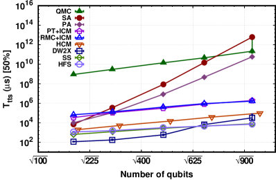
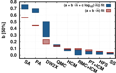
Figure 2: Top panel: computational scaling (for 99% success) for different classical algorithms compared with the experimental results using the DW2X  chip Denchev et al. (2016). As one can see, both general classical algorithms [isoenergetic cluster moves (ICM) either using parallel tempering (PT) or replica Monte Carlo (RMC)] and tailored classical algorithms for the weak-strong cluster model [hybrid cluster moves (HCM), super-spin approximation (SS), Hamze–de-Freitas–Selby (HFS)] have a comparable scaling with the quantum inspired classical algorithm [quantum Monte Carlo (QMC)] and the DW2X  device. com (f). Moreover, for the classical tailored algorithms, the overall scaling prefactor is also comparable with the DW2X  device. For HCM, random instances with no broken qubits have been used. Bottom panel: analysis of the scaling factors by using either linear regression, or a log-corrected regression for $\log_{10}T_{\text{ann}}$. In the figure, bars represent the confidence intervals. For the scaling analysis, we used a stretched exponential that fits better the numerical data (see Appendix A). Interestingly, the general-purposes classical algorithm ICM, together with the chimera-optimized classical algorithm (HFS) and the cluster-optimized algorithms (HCM and SS) have the best scaling. (QMC and SA data taken from Ref. Denchev et al. (2016).) All the simulations (excluding HCM) have been run on the same instances used in Denchev et al. (2016).

IV.2 Non-optimal annealing time and “double scaling”

In the previous section, we analyzed the performance of the various classical and quantum heuristics by looking at the computational scaling. More precisely, we are interested in the asymptotic behavior of the time to solution [see Eq. (4)] that it is expected to be exponential in the limit of large systems:

$$T_{\text{tts}}\approx e^{-b\sqrt{n}},$$ (8)

where $b$ is the asymptotic scaling exponent. However, how large should the system be in order to extrapolate the asymptotic scaling $b$? Many factors such as the annealing schedule Roland and Cerf (2002); Mandrà et al. (2015), as well as the intrinsic noise of the system Mandrà et al. (2015); Shenvi et al. (2003); Roland and Cerf (2005); Amin et al. (2008), can affect the scaling behavior of the computational time. To address the above question, we show in this section that the use of a non-optimal annealing schedule can lead to a “double-scaling” effect where the true asymptotic scaling is hidden by a fictitious (but more favorable) scaling.

It is well known that the computational scaling of a quantum annealer represents only an upper bound of the true scaling if a non-optimal schedule is used Rønnow et al. (2014a); Hen et al. (2015). For instance, consider the case of a fixed schedule but with a very large annealing time. In this case, the computational scaling would be a flat curve because the probability of success would be one for almost all system sizes available for examination. Therefore, very large systems are required to extrapolate to the correct asymptotic scaling.

The DW2X  quantum annealer has a fixed schedule and, as previously mentioned, a minimum annealing time of $20\,\mu$s. Furthermore, the DW2X  chip is affected by an unavoidable intrinsic noise Venturelli et al. (2015); Katzgraber et al. (2015); Zhu et al. (2016); Perdomo-Ortiz et al. (2015a) that can alter the computational scaling.

To better understand the scaling behavior of the DW2X  for the weak-strong cluster model, we compare its scaling with the scaling behavior of a noisy two-energy level model with a fixed (linear) schedule and a non-optimal annealing time. More precisely, we use the following Hamiltonian Roland and Cerf (2002):

$$\mathcal{H}_{\rm 2LV}(t)=-(1-t/T_{\text{ann}})\left|\psi\rangle\!\langle\psi\right|-t/T_{\text{ann}}\left|\omega\rangle\!\langle\omega\right|,$$ (9)

where $T_{\text{ann}}$ is the total annealing time, and $\left|\psi\right\rangle$ and $\left|\omega\right\rangle$ are the equal superposition of all the states and the target states one wants to find, respectively. The system in Eq. (9) can be reduced to an effective $2\times 2$ matrix and, then, it can be exactly solved Roland and Cerf (2002); Mandrà et al. (2015). To simulate the presence of local noise, we assume that each spin has a probability $q$ to be oriented in the wrong direction after the annealing of the system Mandrà et al. (2015). Therefore, the effective noisy Hamiltonian has a probability equal to $(1-q)^{n}$ that its ground state $\omega^{\prime}$ is effectively the desired target state $\omega$. Assuming that the level of noise is small enough compared to the probability of success $p_{\text{succ}}(n,\,T_{\text{ann}})$ of the perfect annealer (namely, when $T_{\text{ann}}$ is much larger than the optimal annealing time), the probability of success of the noisy two-energy level Hamiltonian can be written as:

$$p^{\prime}_{\text{succ}}(n,T_{\text{ann}},\,\,q)=(1-q)^{n}p_{\text{succ}}(n,\,T_{\text{ann}}).$$ (10)

Figure 3 shows the comparison between the computational scaling $T_{\text{tts}}$ for the DW2X  chip Denchev et al. (2016) and the two-energy level model described above (for the numerical details, see Appendix G). For the latter, the computational scaling is expressed in arbitrary units in order to ease the comparison. As expected, the ideal two-energy level model without noise (2LV, $q=0$) has a plateau for small systems and, only for large systems, the computational time shows the asymptotic scaling. When the noise is added to the two-energy level model (2LV, $q=0.1$) a “double scaling” phenomenon appears: for small systems, the scaling is dominated by the noise while, for large systems, the scaling is dominated by the asymptotic scaling. Interestingly, the same phenomenon can be clearly observed for the DW2X  scaling, indicating that the total annealing time of $20\,\mu s$ is non-optimal for systems up to $\sqrt{400}$ spins.

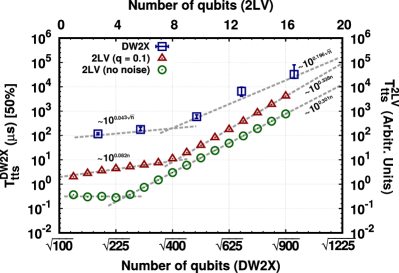
Figure 3: Double-scaling effect produced by the combination of a noisy system and a non-optimal annealing time. We display data for the DW2X  device (as in Denchev et al. (2016)) compared to the annealing of a noisy two-energy level model (2LV) with a non-optimal (linear) annealing schedule and a fixed total annealing time ($T_{\text{ann}}=500$). The numerical study shows that, for small systems, the scaling is mainly dominated by the noise while, for large systems, the scaling is mainly dominated by the asymptotic behavior.

IV.3 Analysis of the energy landscape

An important ingredient in assessing the value of weak-strong cluster problems to detect quantum speedup is to study in detail the dominant characteristics of the energy landscape. In Refs. Yucesoy et al. (2013); Katzgraber et al. (2015) it was shown that the structure of the overlap distribution of spin glasses Binder and Young (1986); Stein and Newman (2013) mirrors salient features in the energy landscape. Because there is no spatial order in spin glasses, “order” is measured by comparing two copies of the system with the same disorder (i.e., the same set of interactions between the qubits and the same magnetic fields), but simulated with independent Markov chains (i.e., each copy starts from a different random initial condition). The spin overlap is defined as

$$q=\frac{1}{n}\sum_{j=1}^{n}\sigma_{j}^{z,\alpha}\sigma_{j}^{z,\beta},$$ (11)

where the sum is over all sites $n$ on the network and $\alpha$ and $\beta$ represent the two copies of the system. For a given set of disorder $J_{\bar{x}\bar{x}^{\prime}}$, the overlap distribution $P(q)$ will have a unique structure at low, but finite temperatures $T\ll J$, $T>0$. Generally speaking, the number of peaks roughly mirrors the number of dominant valleys in the (free-) energy landscape Stein and Newman (2013). The distance between peaks, as well as their width, can be associated with the Hamming distance between dominant valleys and their width, respectively. As shown in Ref. Yucesoy et al. (2013), the more structure the distribution has, the larger the typical computational complexity is. Furthermore, as shown in Ref. Melchert et al. (2016), when the distribution only has one dominant peak, there is either one dominant valley in the energy landscape or a set of strongly-overlapping valleys separated by thin but tall barriers. In the latter case, the barriers are so thin that the features in $P(q)$ overlap strongly, i.e., the distribution cannot differentiate the different valleys. However, if there are multiple well-defined features, dominant valleys in the energy landscape are separated by thick barriers.

Using parallel tempering Monte Carlo at low temperatures Katzgraber et al. (2015), we have computed the overlap distribution for the different weak-strong cluster networks. Because of the added fields, there is no spin-reversal symmetry and the distributions only show peaks for $q>0$. We find two characteristic shapes shown in Figure 4: either the problems have a single dominant narrow peak (compared to random spin-glass problems Katzgraber et al. (2015)), or multiple well-separated peaks. While the latter have energy barriers that are too thick for any finite-range quantum tunneling to be effective, the former potentially have thin enough barriers to allow for finite-range tunneling in the DW2X. Therefore, only problems that have single narrow peaks might benefit from any finite-range tunneling. With better statistics, it would be instructive to study the scaling of both problem classes separately with QMC and SA for systems considerably larger than the DW2X.

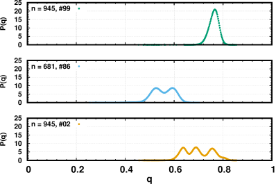
Figure 4: Three representative overlap distributions $P(q)$ for different problem sizes $n$. The $y$-axes are in arbitrary units and rescaled such that $\int_{0}^{1}P(q)=1$. While some instances have either one dominant narrow valley or valleys with thin barriers that allow for finite-range tunneling (top), others have multiple structures (middle and bottom) suggesting that the valleys are separated by barriers that might be too wide for any finite-range tunneling to be beneficial during the optimization.

Figure 5 shows the fraction of problems with multiple peaks against problems with single peaks. The fraction of multi-peak instances (problems with wide barriers in the energy landscape) grows considerably with the problem size $n$, i.e., for large systems the spin-glass backbone dominates and thus, asymptotically, finite-range tunneling becomes inefficient on the DW2X. Loosely extrapolating the data in Fig. 5, we estimate that this class of problem might show a change in scaling already for the next D-Wave chip generation of approximately $2000$ qubits.

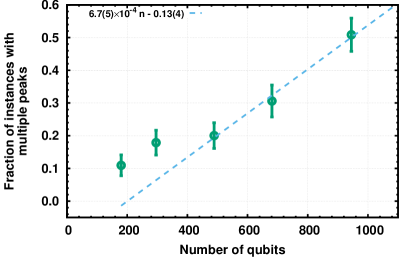
Figure 5: Ratio of single peak to multi-peak overlap distributions as a function of the number of qubits $n$. For increasing system size, multi-peak instances with barriers too wide for finite-range tunneling increase due to the influence of the spin-glass backbone. Note that already for the largest system size studied, multi-valley instances dominate.

Section V Conclusions

In this work, we study in detail and complement recent results by Google Inc. Denchev et al. (2016) on the DW2X  quantum annealer. Their results show for the first time that a quantum annealing machine can outperform conventional computing technologies for a particular class of problems. However, to enable a more detailed comparison, we first expand the notion of “limited quantum speedup” introduced in Ref. Rønnow et al. (2014a). In particular, to perform a fair assessment of the results of Ref. Denchev et al. (2016), we introduce the notion of “limited sequential quantum speedup” which refers to a speedup over the best-known sequential algorithms, as well as“tailored and nontailored quantum speedup.” The latter categories encompass numerical approaches that are not sequential and either exploit the (known) structure of the optimization problem to be solved or are generic. A strong yet fair indication for limited quantum speedup would be to outperform the best-known generic algorithm. In the case of the DW2X  when optimizing the weak-strong cluster networks, our results show that while the DW2X  (as well as quantum Monte Carlo) has a better scaling compared to sequential methods, tailored (as well as nontailored) algorithms show a better asymptotic scaling.

Furthermore, as part of the study, we show that the role of the noise is not marginal in the extrapolation of the asymptotic computational scaling for large system sizes. More precisely, we explain the sudden change of scaling of the computational time of the DW2X  device (and the consequent effect of a “double scaling”) by comparing the quantum annealer with a noisy two-energy level model with a non-optimal annealing schedule. In both cases, the true asymptotic scaling is hidden by an initial (and more favorable) scaling, that later turns to the true asymptotic scaling.

Finally, we study the dominant features in the energy landscape of the weak-strong cluster network problems. Our results suggest that the spin-glass backbone might dominate the scaling already for systems with twice as many qubits as the current-generation DW2X  machine. As such, the favorable speedup currently found both on quantum Monte Carlo simulations as well as the DW2X  device might asymptotically approach towards the scaling of the other sequential methods.

While one might see the results of Ref. Denchev et al. (2016) post a detailed analysis presented in this paper as discouraging, we emphasize that this is a careful study that has shown strong results in favor of quantum annealing approaches both on analog quantum annealing machines, as well as quantum simulations. Although there is a clear evidence that random problems (e.g., spin glasses Rønnow et al. (2014a)) might not be well suited for quantum annealing to excel, tailored problems Katzgraber et al. (2015) are of clear importance in the quest of quantum speedup. Determining the application domain where quantum annealing machines will surpass the capabilities of current silicon-based technologies is of paramount importance across disciplines, and the work by the Google Inc. team has given the first strong indications in which directions to search.

Appendix A Analysis of the computational scaling

In the main text we define the computational time $T_{\text{tts}}$ for a given classical or quantum heuristic as the time to find a solution with $99\%$ probability Rønnow et al. (2014b); Boixo et al. (2014a) as:

$$T_{\text{tts}}=T_{\text{ann}}\frac{\log_{10}(1-s)}{\log_{10}[1-p_{\text{succ}}(T_{\text{ann}})]},$$ (12)

where $s=0.99$, $T_{\text{ann}}$ is annealing/running time and $p_{\text{succ}}(T_{\text{ann}})$ is the probability of success at a given $T_{\text{ann}}$. For the weak-strong cluster model, it is expected that $T_{\text{tts}}$ will scale exponentially with the system size $n$ as

$$T_{\text{tts}}\approx\text{poly}(n)\,10^{a+b\,\sqrt{n}}=10^{a+b\,\sqrt{n}+c\log_{10}\left(\sqrt{n}\right)},$$ (13)

with $n^{c/2}$ is the dominant term of the polynomial prefactor $\text{poly}(n)$. To determine the values of parameters $a$, $b$, and $c$ in Equation (12) we either use a linear fit $f(x)=a+b\,\sqrt{n}$, i.e., it is assumed that the term $c$ is negligible, or a log-corrected fit $f(x)=a+b\,\sqrt{n}+c\log_{10}\left(\sqrt{n}\right)$. In Figure 2 of the main text we report the dominant asymptotic scaling exponent $b$ of $T_{\text{tts}}$ in Equation (4) for the classical or quantum heuristics presented in this paper, while in Fig. 6 we report the values of the parameters $a$ and $c$. Figures 7 and 8 show how well either the linear regression or the log-corrected regression fit the experimental and numerical data, respectively.

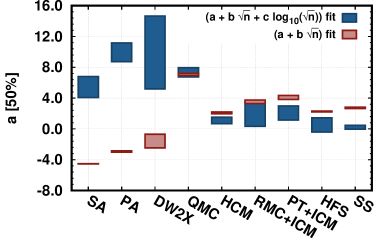
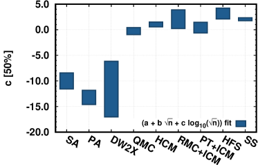
Figure 6: Values for the remaining fit parameters $a$ and $c$ for either the log-corrected fit $a+b\sqrt{n}+c\log_{10}(\sqrt{n})$ or the linear fit $a+b\sqrt{n}$. In the panels, bars represent the confidence interval.

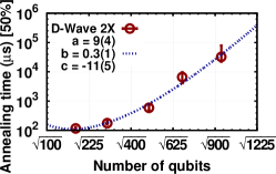
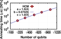
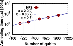
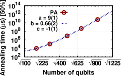
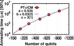
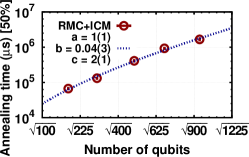
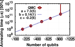
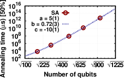
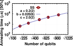
Figure 7: Scaling analysis of $\log_{10}T_{\text{ann}}$ by using a log-corrected fit of the form $f(n)=a+b\sqrt{n}+c\log_{10}(\sqrt{n})$, where $n$ is the number of qubits. The panels show the values of the fit parameters and how well the function $f(n)$ fits the data.

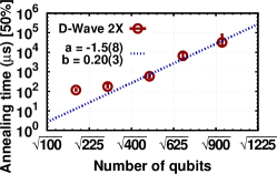
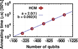
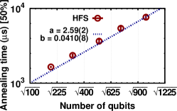
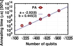
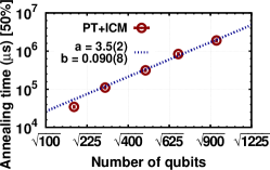
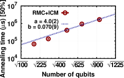
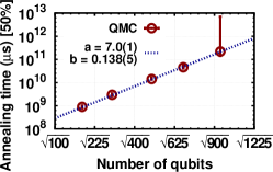
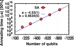
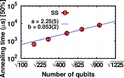
Figure 8: Scaling analysis of $\log_{10}T_{\text{ann}}$ by using a linear fit of the form $f(n)=a+b\sqrt{n}$, where $n$ is the number of qubits. The panels show the values of the fit parameters and how well $f(n)$ fits the data. For the fit, only the last three data points are used.

Appendix B Hybrid Cluster Method (HCM)

The hybrid cluster method (HCM) is a Metropolis sampling technique where “clusters” are updated instead of single spins. The outline of HCM is simple: given a set of connected $K$ spin-domains $\{\mathcal{D}_{i}\}_{i=1,\,\ldots,\,K}$ such that their union is the whole system, clusters are created using the Wolff rule Wolff (1989) inside a randomly-chosen domain $\mathcal{D}_{i}$. Then the cluster is flipped by following a Metropolis updated by considering only couplings outside the selected domain (see Ref. Venturelli et al. (2015) for more details). HCM was initially developed to improve the thermalization of highly-structured systems such as embedded systems because it preserves the detailed balance Venturelli et al. (2015) condition. Additionally, HCM can be used as a random heuristics for finding ground states efficiently.

In the weak-strong cluster model, domains $\mathcal{D}_{i}$ are identified as unit cells of the chimera graph. Because spins inside unit cells are ferromagnetically coupled, they are likely to act as a single cluster in the low-temperature regime. The system is therefore started from an initial high temperature $1/T_{\text{ini}}=\beta_{\text{ini}}=0.5$ and then cooled to the final temperature $1/T_{\text{end}}=\beta_{\text{end}}=3$. For the simulations, a linear schedule (in the inverse temperature $\beta$) with $M$ steps has been used, where $M$ is optimized by minimizing Eq. (12). At each step, a full update of the system is made.

Table 1 lists the simulation parameters used to compute the time to solution in Fig. 2 of the main text.

Table 1: Parameters of the simulation using the hybrid cluster method (HCM) on the chimera topology. $M$ represents the optimal number of inverse temperature steps for the thermal annealing.

System size ($n$)	$\beta_{\text{ini}}$	$\beta_{\text{end}}$	$M$
$192$	$0.5$	$3$	$5$
$300$	$0.5$	$3$	$6$
$520$	$0.5$	$3$	$8$
$720$	$0.5$	$3$	$11$
$992$	$0.5$	$3$	$14$

Appendix C Isoenergetic Cluster Algorithm (ICM)

The isoenergetic cluster method (ICM) is a rejection-free cluster algorithm for spin glasses that greatly improves thermalization Zhu et al. (2015). The main idea of ICM consists in restricting Houdayer cluster moves Houdayer (2001) to temperatures where cluster percolation is hampered by the interplay of frustration and temperature. As such, one is able to extend the Houdayer cluster algorithm from two-dimensional spin glasses (for which the Houdayer algorithm was originally designed for) to any topology and/or space dimension. More precisely, $M$ copies of the system are run at the same temperature. The $q$-space intersection between two random replicas $\alpha$ and $\beta$ is then defined as $q_{j}=\sigma^{z,\alpha}_{j}\sigma^{z,\beta}_{j}$ Zhu et al. (2015). Within the overlap space ($q$-space) the system has two domains: sites with $q_{j}=1$ and the sites with $q_{j}=-1$. In ICM, clusters are defined as the connected parts of these domains. Once the clusters are created, a random site with $q_{j}=-1$ is chosen and the corresponding cluster flipped. Because the total energy of the two copies of the system is unchanged by this transformation, the acceptance of the cluster move is rejection free. One of the main advantages of ICM is that it allows for a more extensive exploration of the energy landscape by classically teleporting across energy barriers. Note that the cluster updates obey detailed balance and are only ergodic after being combined with Monte Carlo lattice sweeps. The method is used to improve the sampling of parallel tempering Monte Carlo (PT) Hukushima and Nemoto (1996); Katzgraber et al. (2004); Katzgraber (2009) which is the current state-of-the-art simulation method for spin glasses.

Although the aforementioned approach is designed to quickly thermalize a frustrated system at finite temperatures, the method can be adjusted to act as a heuristic to find ground state configurations Katzgraber and Young (2003); Moreno et al. (2003) (PT+ICM). To do this, the lowest temperature of the simulation is chosen low enough such that the different copies of the system at different temperatures occasionally dip into the ground state. To verify whether the true ground state has been reached, two criteria are adopted: first, the same minimum-energy state has to be reached from four replicas at the minimum temperature $T_{\rm min}$. Second, this state has to be reached during the first $25$% of the sweeps in all four copies. These conditions are satisfied for the parameters listed in Table 2.

We have also combined ICM with the replica Monte Carlo algorithm (RMC+ICM) Wang and Swendsen (2005). The RMC algorithm is based on three basic steps: first, $R$ replicas of the system are run at different temperatures $\{T_{1},T_{2},...,T_{R}\}$. Second, a site is picked at random and the associated cluster (which is defined through the overlap of the systems at nearby temperatures) is created. Third, a Metropolis update is performed to flip the cluster. Replica Monte Carlo is extremely efficient in two-dimensional or quasi-two-dimensional spin glasses, reducing the correlation time enormously compared to single spin flips Wang and Swendsen (2005). However, in higher space dimensions, its performance is comparable to parallel tempering Monte Carlo. The parameters for the simulations are reported in Table 2.

Table 2: Parameters of the simulation using the isoenergetic cluster method (ICM) on the chimera topology. $T_{\text{min}}$ [$T_{\text{max}}$] is the lowest [highest] temperature simulated, and $N_{T}$ is the total number of temperatures used in the parallel tempering and replica Monte Carlo methods. Isoenergetic cluster moves only occur for the lowest $N_{\text{c}}$ temperatures simulated.

System size ($n$)	$T_{\text{min}}$	$T_{\text{max}}$	$N_{T}$	$N_{\text{c}}$
$180,\,296,\,489,\,681,\,945$	$0.2279$	$2.5000$	$21$	$5$

Appendix D Population Annealing Monte Carlo (PA)

Population annealing (PA) Monte Carlo is a sequential Monte Carlo algorithm to compute equilibrium states of systems with rugged energy landscapes Hukushima and Iba (2003); Machta (2010); Machta and Ellis (2011); Wang et al. (2015a, b). PA is closely related to simulated annealing in that the system is prepared at a high temperature and then annealed to a low target temperature. However, instead of simulating one system, in population annealing $R$ copies of the system are simulated in parallel. At each temperature step the population of replicas is resampled such that they represent (at any temperature) a faithful Boltzmann distribution for that given temperature. Once the replicas have been resampled, replicas are updated using Metropolis sampling. In Ref. Wang et al. (2015a) it was shown that PA can be used as an optimization heuristic that clearly outperforms simulated annealing.

Table 3: Simulation parameters for population annealing Monte Carlo (PA): number of spins $n$, working population size $R$, number of temperatures $N_{T}$, and number of independent runs $M$. For all the simulations, temperatures are evenly chosen in the interval $\beta=[0,\,1]$ and the number of sweeps applied to each replica is fixed to $N_{S}=10$.

System size ($n$)	$R$	$N_{T}$	$M$
$180$	$10^{2}$	$100$	$200$
$296$	$3\cdot 10^{2}$	$100$	$200$
$489$	$10^{4}$	$200$	$200$
$681$	$10^{5}$	$300$	$200$
$945$	$3\cdot 10^{6}$	$300$	$\phantom{2}55$

In the actual simulations we simulate each problem at a working population of size $R$ and measure the success probability $p$ to find the ground states via $M$ independent runs. The probability $p$ is then used to calculate the critical population size $R_{c}$ for a $99\%$ success probability as $R_{c}=R\,\ln(0.01)/\ln(1-p)$. This can be further transformed to the amount of work in Monte Carlo lattice sweeps, and thus a physical time. Here, we use $N_{T}$ temperatures evenly distributed in $\beta=1/T\in[0,\,1]$, and at each temperature, $N_{S}=10$ Monte Carlo sweeps are applied to each replica. Table 3 lists the parameters of the simulation.

Appendix E Super-spin heuristic (SS)

The weak-strong cluster model introduced in Ref. Denchev et al. (2016) is a highly-structured problem. In particular, $\text{K}_{4,4}$ unit cells of the chimera graph are ferromagnetically coupled and biased by a strong external field. Hence, spins belonging to the same unit cell are likely to be aligned in the ground state. The super-spin (SS) approach takes advantage of the structure of the weak-strong clusters by identifying a single $\text{K}_{4,4}$ cell as a “super-spin”. The resulting “logical” model is therefore a considerably smaller two-dimensional spin-glass problems with external fields. Each of these logical spins is then coupled to an external local field. For the example shown in Figure 1, the original problem size of $n=224$ spins is reduced to a spin-glass problem of only $224/8=28$ spins that is trivial to optimize.

The time-to-solution of the SS approximation is then computed by applying the ICM+PT heuristic introduced in Appendix C. Because the SS approximation does not take into account the detailed structure of the strong-weak clusters, it is expected to be the fastest among the different heuristics used. Indeed, as shown in Fig. 2, results using SS are not only the fastest, but also represent the algorithm with the best computational scaling.

Appendix F Other algorithms used (QMC, SA, and HFS)

For details on the quantum Monte Carlo (QMC) and simulated annealing (SA) results, simulation parameters and algorithmic details we refer the reader to Ref. Denchev et al. (2016). The Hamze–de-Freitas–Selby (HFS) algorithm Hamze and de Freitas (2004); Selby (2014) is explained in detail in Ref. com (g).

Appendix G Two-energy level system

The calculation of the probability of success $p_{\text{succ}}(n,\,T_{\text{ann}})$ for the two-energy level model in Eq. (9) has been done by a numerical integration of the Schrödinger equation using a a non-optimal (linear) schedule with a total annealing time of $T_{\text{ann}}=500$. For the integration, we have discretized the time using $\delta t=0.01$ for all the system sizes $n={1,\,2,\,\ldots,\,16}$. The time discretization has been chosen so that there were no appreciable changes in $p_{\text{succ}}(n,\,T_{\text{ann}})$ by decreasing $\delta t$. Table 4 reports the parameters used for the two-energy level model.

Table 4: Parameters used for the numerical integration of the Schrödinger equation of the two-energy level model in Equation (9).

System size ($n$)	Schedule	$T_{\text{max}}$	$\delta t$
$1,\,2,\,\ldots,\,16$	linear	$500$	$0.01$

References

- Nielsen and Chuang (2000) M. A. Nielsen and I. L. Chuang, Quantum Computation and Quantum Information (Cambridge University Press, Cambridge, 2000).
- Nishimori (2001) H. Nishimori, Statistical Physics of Spin Glasses and Information Processing: An Introduction (Oxford University Press, New York, 2001).
- Finnila et al. (1994) A. B. Finnila, M. A. Gomez, C. Sebenik, C. Stenson, and J. D. Doll, Quantum annealing: A new method for minimizing multidimensional functions, Chem. Phys. Lett. 219, 343 (1994).
- Kadowaki and Nishimori (1998) T. Kadowaki and H. Nishimori, Quantum annealing in the transverse Ising model, Phys. Rev. E 58, 5355 (1998).
- Brooke et al. (1999) J. Brooke, D. Bitko, T. F. Rosenbaum, and G. Aepli, Quantum annealing of a disordered magnet, Science 284, 779 (1999).
- Farhi et al. (2000) E. Farhi, J. Goldstone, S. Gutmann, and M. Sipser, Quantum Computation by Adiabatic Evolution (2000), arXiv:quant-ph/0001106.
- Roland and Cerf (2002) J. Roland and N. J. Cerf, Quantum search by local adiabatic evolution, Phys. Rev. A 65, 042308 (2002).
- Santoro et al. (2002) G. Santoro, E. Martoňák, R. Tosatti, and R. Car, Theory of quantum annealing of an Ising spin glass, Science 295, 2427 (2002).
- Das and Chakrabarti (2005) A. Das and B. K. Chakrabarti, Quantum Annealing and Related Optimization Methods (Edited by A. Das and B.K. Chakrabarti, Lecture Notes in Physics 679, Berlin: Springer, 2005).
- Santoro and Tosatti (2006) G. E. Santoro and E. Tosatti, TOPICAL REVIEW: Optimization using quantum mechanics: quantum annealing through adiabatic evolution, J. Phys. A 39, R393 (2006).
- Lidar (2008) D. A. Lidar, Towards Fault Tolerant Adiabatic Quantum Computation, Phys. Rev. Lett. 100, 160506 (2008).
- Das and Chakrabarti (2008) A. Das and B. K. Chakrabarti, Quantum Annealing and Analog Quantum Computation, Rev. Mod. Phys. 80, 1061 (2008).
- Morita and Nishimori (2008) S. Morita and H. Nishimori, Mathematical Foundation of Quantum Annealing, J. Math. Phys. 49, 125210 (2008).
- Mukherjee and Chakrabarti (2015) S. Mukherjee and B. K. Chakrabarti, Multivariable optimization: Quantum annealing and computation, Eur. Phys. J. Special Topics 224, 17 (2015).
- Kirkpatrick et al. (1983) S. Kirkpatrick, C. D. Gelatt, Jr., and M. P. Vecchi, Optimization by simulated annealing, Science 220, 671 (1983).
- com (a) URL http://www.dwavesys.com.
- Johnson et al. (2011) M. W. Johnson, M. H. S. Amin, S. Gildert, T. Lanting, F. Hamze, N. Dickson, R. Harris, A. J. Berkley, J. Johansson, P. Bunyk, et al., Quantum annealing with manufactured spins, Nature 473, 194 (2011).
- Dickson et al. (2013) N. G. Dickson, M. W. Johnson, M. H. Amin, R. Harris, F. Altomare, A. J. Berkley, P. Bunyk, J. Cai, E. M. Chapple, P. Chavez, et al., Thermally assisted quantum annealing of a 16-qubit problem, Nat. Commun. 4, 1903 (2013).
- Pudenz et al. (2014) K. L. Pudenz, T. Albash, and D. A. Lidar, Error-corrected quantum annealing with hundreds of qubits, Nat. Commun. 5, 3243 (2014).
- Smith and Smolin (2013) G. Smith and J. Smolin, Putting “Quantumness” to the Test, Physics 6, 105 (2013).
- Boixo et al. (2013) S. Boixo, T. Albash, F. M. Spedalieri, N. Chancellor, and D. A. Lidar, Experimental signature of programmable quantum annealing, Nat. Commun. 4, 2067 (2013).
- Rønnow et al. (2014a) T. F. Rønnow, Z. Wang, J. Job, S. Boixo, S. V. Isakov, D. Wecker, J. M. Martinis, D. A. Lidar, and M. Troyer, Defining and detecting quantum speedup (2014a), (arXiv:quant-phys/1401.2910).
- Katzgraber et al. (2014) H. G. Katzgraber, F. Hamze, and R. S. Andrist, Glassy Chimeras Could Be Blind to Quantum Speedup: Designing Better Benchmarks for Quantum Annealing Machines, Phys. Rev. X 4, 021008 (2014).
- Lanting et al. (2014) T. Lanting, A. J. Przybysz, A. Y. Smirnov, F. M. Spedalieri, M. H. Amin, A. J. Berkley, R. Harris, F. Altomare, S. Boixo, P. Bunyk, et al., Entanglement in a quantum annealing processor, Phys. Rev. X 4, 021041 (2014).
- Santra et al. (2014) S. Santra, G. Quiroz, G. Ver Steeg, and D. A. Lidar, Max 2-SAT with up to 108 qubits, New J. Phys. 16, 045006 (2014).
- Shin et al. (2014) S. W. Shin, G. Smith, J. A. Smolin, and U. Vazirani, How “Quantum” is the D-Wave Machine? (2014), (arXiv:1401.7087).
- Boixo et al. (2014a) S. Boixo, T. F. Rønnow, S. V. Isakov, Z. Wang, D. Wecker, D. A. Lidar, J. M. Martinis, and M. Troyer, Evidence for quantum annealing with more than one hundred qubits, Nat. Phys, 10, 218 (2014a).
- Albash et al. (2015a) T. Albash, W. Vinci, A. Mishra, P. A. Warburton, and D. A. Lidar, Consistency Tests of Classical and Quantum Models for a Quantum Device, Phys. Rev. A 91, 042314 (2015a).
- Albash et al. (2015b) T. Albash, T. F. Rønnow, M. Troyer, and D. A. Lidar, Reexamining classical and quantum models for the D-Wave One processor, Eur. Phys. J. Spec. Top. 224, 111 (2015b).
- Katzgraber et al. (2015) H. G. Katzgraber, F. Hamze, Z. Zhu, A. J. Ochoa, and H. Munoz-Bauza, Seeking Quantum Speedup Through Spin Glasses: The Good, the Bad, and the Ugly, Phys. Rev. X 5, 031026 (2015).
- Martin-Mayor and Hen (2015) V. Martin-Mayor and I. Hen, Unraveling Quantum Annealers using Classical Hardness (2015), (arXiv:1502.02494).
- Pudenz et al. (2015) K. L. Pudenz, T. Albash, and D. A. Lidar, Quantum Annealing Correction for Random Ising Problems, Phys. Rev. A 91, 042302 (2015).
- Hen et al. (2015) I. Hen, J. Job, T. Albash, T. F. Rønnow, M. Troyer, and D. A. Lidar, Probing for quantum speedup in spin-glass problems with planted solutions, Phys. Rev. A 92, 042325 (2015).
- Venturelli et al. (2015) D. Venturelli, S. Mandrà, S. Knysh, B. O’Gorman, R. Biswas, and V. Smelyanskiy, Quantum Optimization of Fully Connected Spin Glasses, Phys. Rev. X 5, 031040 (2015).
- Vinci et al. (2015) W. Vinci, T. Albash, G. Paz-Silva, I. Hen, and D. A. Lidar, Quantum annealing correction with minor embedding, Phys. Rev. A 92, 042310 (2015).
- Zhu et al. (2016) Z. Zhu, A. J. Ochoa, F. Hamze, S. Schnabel, and H. G. Katzgraber, Best-case performance of quantum annealers on native spin-glass benchmarks: How chaos can affect success probabilities, Phys. Rev. A 93, 012317 (2016).
- Bunyk et al. (2014) P. Bunyk, E. Hoskinson, M. W. Johnson, E. Tolkacheva, F. Altomare, A. J. Berkley, R. Harris, J. P. Hilton, T. Lanting, and J. Whittaker, Architectural Considerations in the Design of a Superconducting Quantum Annealing Processor, IEEE Trans. Appl. Supercond. 24, 1 (2014).
- Lidar and Brun (2013) D. A. Lidar and T. A. Brun, eds., Quantum Error Correction (Cambridge University Press, Cambride, UK, 2013).
- Perdomo-Ortiz et al. (2015a) A. Perdomo-Ortiz, B. O’Gorman, J. Fluegemann, R. Biswas, and V. N. Smelyanskiy, Determination and correction of persistent biases in quantum annealers (2015a), (arXiv:quant-phys/1503.05679).
- Perdomo-Ortiz et al. (2015b) A. Perdomo-Ortiz, J. Fluegemann, R. Biswas, and V. N. Smelyanskiy, A Performance Estimator for Quantum Annealers: Gauge selection and Parameter Setting (2015b), (arXiv:quant-phys/1503.01083).
- Binder and Young (1986) K. Binder and A. P. Young, Spin Glasses: Experimental Facts, Theoretical Concepts and Open Questions, Rev. Mod. Phys. 58, 801 (1986).
- Stein and Newman (2013) D. L. Stein and C. M. Newman, Spin Glasses and Complexity, Primers in Complex Systems (Princeton University Press, 2013).
- Isakov et al. (2015) S. V. Isakov, I. N. Zintchenko, T. F. Rønnow, and M. Troyer, Optimized simulated annealing for Ising spin glasses, Comput. Phys. Commun. 192, 265 (2015), (see also ancillary material to arxiv:cond-mat/1401.1084).
- Isakov et al. (2014) S. V. Isakov, I. N. Zintchenko, T. F. Rønnow, and M. Troyer, Optimized simulated annealing for Ising spin glasses (2014), (ancillary material to arxiv:cond-mat/1401.1084).
- com (b) Note that the “slight” advantage found in Ref. Katzgraber et al. (2015) for the D-Wave Two quantum annealer over classical simulated annealing has to be seen in a relative sense. While the D-Wave Two quantum annealer failed to solve most problems, it performed better for problems with thinner energy barriers. Furthermore, if the criterion for success is relaxed to include the lowest energy states, the performance of the D-Wave Two improved noticeably in comparison to classical simulated annealing.
- Lucas (2014) A. Lucas, Ising formulations of many NP problems, Front. Physics 12, 5 (2014).
- Denchev et al. (2016) V. S. Denchev, S. Boixo, S. V. Isakov, N. Ding, R. Babbush, V. Smelyanskiy, J. Martinis, and H. Neven, What is the Computational Value of Finite Range Tunneling?, Phys. Rev. X 6, 031015 (2016).
- Suzuki (1993) M. Suzuki, Quantum Monte Carlo Methods in Condensed Matter Physics (World Scientific, Singapore, 1993).
- Hartmann and Rieger (2001) A. K. Hartmann and H. Rieger, Optimization Algorithms in Physics (Wiley-VCH, Berlin, 2001).
- Elf et al. (2001) M. Elf, C. Gutwenger, M. Jünger, and G. Rinaldi, Lecture notes in computer science 2241, in Computational Combinatorial Optimization, edited by M. Jünger and D. Naddef (Springer Verlag, Heidelberg, 2001), vol. 2241.
- Hartmann and Rieger (2004) A. K. Hartmann and H. Rieger, New Optimization Algorithms in Physics (Wiley-VCH, Berlin, 2004).
- Zhu et al. (2015) Z. Zhu, A. J. Ochoa, and H. G. Katzgraber, Efficient Cluster Algorithm for Spin Glasses in Any Space Dimension, Phys. Rev. Lett. 115, 077201 (2015).
- Boixo et al. (2014b) S. Boixo, V. N. Smelyanskiy, A. Shabani, S. V. Isakov, M. Dykman, V. S. Denchev, M. Amin, A. Smirnov, M. Mohseni, and H. Neven, Computational Role of Collective Tunneling in a Quantum Annealer (2014b), arXiv:1411.4036.
- Boixo et al. (2016) S. Boixo, V. N. Smelyanskiy, A. Shabani, S. V. Isakov, M. Dykman, V. S. Denchev, M. H. Amin, A. Y. Smirnov, M. Mohseni, and H. Neven, Computational multiqubit tunnelling in programmable quantum annealers, Nat. Comm. 7, 10327 (2016).
- Rønnow et al. (2014b) T. F. Rønnow, Z. Wang, J. Job, S. Boixo, S. V. Isakov, D. Wecker, J. M. Martinis, D. A. Lidar, and M. Troyer, Defining and detecting quantum speedup, Science 345, 420 (2014b).
- com (c) A simple analogy is the following: Suppose the reader wants to compare two motorbikes. Surely, it would make no sense to race a dirt bike against a superbike on a dirt road, because the slicks on the superbike would have no traction on dirt. Similarly, racing the dirt bike against a superbike on a paved racetrack would be futile, because the dirt bike would have little to no grip on the pavement. Therefore, it is important to introduce categories where the individual types of motorbikes are compared, i.e., motocross and the superbike series.
- Grover (1997) L. K. Grover, Quantum mechanics helps in searching for a needle in a haystack, Phys. Rev. Lett. 79, 3258 (1997).
- Papageorgiou and Traub (2013) A. Papageorgiou and J. F. Traub, Measures of quantum computing speedup, Phys. Rev. A 88, 022316 (2013).
- Shor (1997) P. W. Shor, Polynomial-time algorithms for prime factorization and discrete logarithms on a quantum computer, SIAM J. Comp. 26, 1484 (1997).
- Hukushima and Iba (2003) K. Hukushima and Y. Iba, in The Monte Carlo method in the physical sciences: celebrating the 50th anniversary of the Metropolis algorithm, edited by J. E. Gubernatis (AIP, 2003), vol. 690, p. 200.
- Machta (2010) J. Machta, Population annealing with weighted averages: A Monte Carlo method for rough free-energy landscapes, Phys. Rev. E 82, 026704 (2010).
- Wang et al. (2015a) W. Wang, J. Machta, and H. G. Katzgraber, Comparing Monte Carlo methods for finding ground states of Ising spin glasses: Population annealing, simulated annealing, and parallel tempering, Phys. Rev. E 92, 013303 (2015a).
- Wang et al. (2015b) W. Wang, J. Machta, and H. G. Katzgraber, Population annealing: Theory and application in spin glasses, Phys. Rev. E 92, 063307 (2015b).
- Zintchenko et al. (2015) I. Zintchenko, M. B. Hastings, and M. Troyer, From local to global ground states in Ising spin glasses, Phys. Rev. B 91, 024201 (2015).
- Hamze and de Freitas (2004) F. Hamze and N. de Freitas, in Proceedings of the 20th Conference on Uncertainty in Artificial Intelligence (AUAI Press, Arlington, Virginia, United States, 2004), UAI ’04, p. 243, ISBN 0-9749039-0-6.
- Selby (2014) A. Selby, Efficient subgraph-based sampling of Ising-type models with frustration (2014), (arXiv:cond-mat/1409.3934).
- com (d) Note that some algorithms might share elements from multiple categories. In this case, it will be difficult to define the type of speedup. However, one should keep in mind that the goal is to make the fairest comparison possible.
- Matsuda et al. (2009) Y. Matsuda, H. Nishimori, and H. G. Katzgraber, Ground-state statistics from annealing algorithms: quantum versus classical approaches, New J. Phys. 11, 073021 (2009).
- Crosson et al. (2014) E. Crosson, E. Farhi, C. Yen-Yu Lin, H.-H. Lin, and P. Shor, Different Strategies for Optimization Using the Quantum Adiabatic Algorithm (2014), (arXiv:quant-phys/1401.7320).
- Perdomo-Ortiz et al. (2011) A. Perdomo-Ortiz, S. E. Venegas-Andraca, and A. Aspuru-Guzik, A study of heuristic guesses for adiabatic quantum computation, Quant, Inf. Proc. 10, 33 (2011).
- com (e) M. Troyer, private communication.
- com (f) Simulations using the groups approach Zintchenko et al. (2015) show a similar scaling to HCM and ICM, but are slower than the HFS and SS algorithms.
- Mandrà et al. (2015) S. Mandrà, G. G. Guerreschi, and A. Aspuru-Guzik, Adiabatic quantum optimization in the presence of discrete noise: Reducing the problem dimensionality, Phys. Rev. A 92, 062320 (2015).
- Shenvi et al. (2003) N. Shenvi, K. R. Brown, and K. B. Whaley, Effects of noisy oracle on search algorithm complexity, Phys. Rev. A 68, 052313 (2003).
- Roland and Cerf (2005) J. Roland and N. J. Cerf, Noise resistance of adiabatic quantum computation using random matrix theory, Phys. Rev. A 71, 032330 (2005).
- Amin et al. (2008) M. H. S. Amin, P. J. Love, and C. J. S. Truncik, Thermally assisted adiabatic quantum computation, Phys. Rev. Lett 100, 060503 (2008).
- Yucesoy et al. (2013) B. Yucesoy, J. Machta, and H. G. Katzgraber, Correlations between the dynamics of parallel tempering and the free-energy landscape in spin glasses, Phys. Rev. E 87, 012104 (2013).
- Melchert et al. (2016) O. Melchert, H. G. Katzgraber, and M. A. Novotny, Site- and bond-percolation thresholds in -based lattices: Vulnerability of quantum annealers to random qubit and coupler failures on chimera topologies, Phys. Rev. E 93, 042128 (2016).
- Wolff (1989) U. Wolff, Collective Monte Carlo updating for spin systems, Phys. Rev. Lett. 62, 361 (1989).
- Houdayer (2001) J. Houdayer, A cluster Monte Carlo algorithm for 2-dimensional spin glasses, Eur. Phys. J. B. 22, 479 (2001).
- Hukushima and Nemoto (1996) K. Hukushima and K. Nemoto, Exchange Monte Carlo method and application to spin glass simulations, J. Phys. Soc. Jpn. 65, 1604 (1996).
- Katzgraber et al. (2004) H. G. Katzgraber, S. Trebst, D. Huse, and M. Troyer, Feedback-optimized parallel tempering Monte Carlo (2004), (unpublished).
- Katzgraber (2009) H. G. Katzgraber, Introduction to Monte Carlo Methods (2009), (arXiv:0905.1629).
- Katzgraber and Young (2003) H. G. Katzgraber and A. P. Young, Monte Carlo studies of the one-dimensional Ising spin glass with power-law interactions, Phys. Rev. B 67, 134410 (2003).
- Moreno et al. (2003) J. J. Moreno, H. G. Katzgraber, and A. K. Hartmann, Finding low-temperature states with parallel tempering, simulated annealing and simple Monte Carlo, Int. J. Mod. Phys. C 14, 285 (2003).
- Wang and Swendsen (2005) J.-S. Wang and R. H. Swendsen, Replica Monte Carlo Simulation (Revisited), Prog. Theor. Phys. Supplement 157, 317 (2005).
- Machta and Ellis (2011) J. Machta and R. Ellis, Monte Carlo Methods for Rough Free Energy Landscapes: Population Annealing and Parallel Tempering, J. Stat. Phys. 144, 541 (2011).
- com (g) URL http://wp.me/PRVXj-4g.