Multiple network alignment via multiMAGNA++

Abstract

Motivation: Network alignment (NA) aims to find a node mapping between molecular networks of different species that identifies topologically or functionally similar network regions. Analogous to genomic sequence alignment, NA can be used to transfer biological knowledge from well- to poorly-studied species between aligned network regions. Pairwise NA (PNA) finds similar regions between two networks while multiple NA (MNA) can align more than two networks. We focus on MNA. Existing MNA methods aim to maximize total similarity over all aligned nodes (node conservation). Then, they evaluate alignment quality by measuring the amount of conserved edges, but only after the alignment is constructed. Directly optimizing edge conservation during alignment construction in addition to node conservation may result in superior alignments.
Results: Thus, we present a novel MNA approach called multiMAGNA++ that can achieve this. Indeed, multiMAGNA++ generally outperforms or is on par with the existing MNA methods, while often completing faster than the existing methods. That is, multiMAGNA++ scales well to larger network data and can be parallelized effectively. During method evaluation, we also introduce new MNA quality measures to allow for more complete alignment characterization as well as more fair MNA method comparison compared to using only the existing alignment quality measures.
Code availability: Code is available upon request.
Contact: tmilenko@nd.edu

1 Introduction

Networks can model a variety of real-world systems, including biological ones. Many networks are relevant to biological systems, such as protein-protein interaction (PPI) (Breitkreutz et al., 2008), gene co-expression (Stuart et al., 2003), or metabolic (Jeong et al., 2000) networks. In PPI networks, nodes are proteins and edges are physical interactions between the proteins. The interactions between the proteins control and carry out complex cellular functions, and hence, studying PPI networks is important. Biotechnological advances have made PPI network data available for many species (Breitkreutz et al., 2008). Functions of many proteins in many species remain unknown (Sharan et al., 2007; Mulder et al., 2014), and hence, there is need for across-species transfer of existing functional knowledge from well-studied species to poorly-studied ones. Typically, genomic sequence alignment has been used for this purpose (Ye et al., 2006). However, since proteins interact in the cell to carry out cellular function and since PPI networks model these interactions (whereas sequence alignment studies genes in isolation), biological network alignment (NA) can be used for this knowledge transfer too, in order to complement the biological insights that have already been gained via sequence alignment.

NA aims to find a node mapping between networks that identifies topologically or functionally similar network regions. As such, NA can be used to transfer biological knowledge across species between the species’ conserved (aligned) PPI network regions (Sharan and Ideker, 2006a). While we focus on NA of PPI networks and on the domain of computational biology (Sharan and Ideker, 2006b; Clark and Kalita, 2014; Faisal et al., 2015), NA is applicable to any network type (e.g., gene regulatory or metabolic networks) and a wide number of fields (e.g., pattern recognition (Conte et al., 2004; Torresani et al., 2008), language processing (Bayati et al., 2009), social networks (Koutra et al., 2013; Kollias et al., 2012), and computer vision (Duchenne et al., 2011)).

NA is related to the subgraph isomorphism problem, which asks whether one network (or graph) is an exact subgraph of another network. The subgraph isomorphism problem is NP-complete, meaning that there is no efficient method to solve it exactly for large input networks. NA is a more general problem as it asks how to best “fit” one network into another network, even if the first network is not an exact subgraph of the second one. It is not obvious how to measure the quality of the fit of one network into another one. But a measure that is widely used quantifies the amount of conserved (aligned) edges, or in other words, the size of the common conserved subgraph between the aligned networks. Maximizing edge conservation is NP-hard (Kuchaiev and Pržulj, 2011). Thus, heuristic methods need to be sought for NA.

NA can be either local or global (see Meng et al. (2015); Faisal et al. (2015); Elmsallati et al. (2015) for a review). Initial NA focus was on local NA, which finds smaller, highly conserved regions, e.g., biological pathways or protein complexes, among networks. However, local NA does not generally capture large conserved subgraphs, and the aligned regions can overlap, leading to an ambiguous (from a mathematical perspective) many-to-many node mapping. More recent efforts have focused on global NA, which maps entire networks to each other. Since global NA can find large conserved subgraphs shared by the aligned networks, and since large conserved subgraphs have been argued to be more helpful in aiding transfer of knowledge between networks (Milenković et al., 2010; Patro and Kingsford, 2012), we focus on global NA.

NA can be classified in another way: as pairwise NA (PNA) or multiple NA (MNA). PNA finds similar regions between two networks while MNA can align more than two networks. PNA typically produces an injective (one-to-one) node mapping between two networks, which results in aligned node pairs. MNA produces an alignment consisting of aligned node clusters. Given an alignment of multiple networks, if an aligned cluster contains more than one node from a single network, it is a many-to-many MNA. If there is a maximum of one node per network in every aligned cluster, it is a one-to-one MNA. While MNA may lead to deeper biological insights compared to PNA since it captures at once functional knowledge that is common to multiple species, which is why we focus on MNA, MNA is computationally much harder than PNA since the complexity of the NA problem increases exponentially with the number of networks to be aligned.

Existing global NA methods are typically two-stage aligners: they first calculate similarity (with respect to some node cost function) between nodes from different networks, and then they use an alignment strategy to identify high scoring alignments with respect to the total similarity over all aligned nodes (also known as node conservation). Examples of two-stage PNA methods are IsoRank (Singh et al., 2007), GHOST (Patro and Kingsford, 2012), and the GRAAL family of methods (Kuchaiev et al., 2010; Milenković et al., 2010; Kuchaiev and Pržulj, 2011). Examples of two-stage MNA methods are IsoRankN (Liao et al., 2009), MI-Iso (Faisal et al., 2014), SMETANA (Sahraeian and Yoon, 2013), BEAMS (Alkan and Erten, 2014), NetCoffee (Hu et al., 2014), CSRW (Jeong and Yoon, 2015), and FUSE (Gligorijević et al., 2015). For an overview of these methods, see Section A.

Faisal et al. (2014) and Crawford et al. (2015) pointed out a key issue with two-stage NA methods. Namely, they evaluated these methods by mixing and matching their node cost functions and alignment strategies. They showed that node cost function of one method and alignment strategy of another method can (and typically do) yield a new superior method. This finding highlighted the need for properly evaluating a new two-stage NA method against the existing ones, by using the above mix-and-match strategy, in order to determine whether it is the new method’s node cost function or its alignment strategy (or both) that leads to its potential superiority.

Another important issue that exists with the two-stage NA methods is as follows. Once the two-stage NA methods generate an alignment that has high node conservation, they typically evaluate the quality of the alignment using some other measure that is different from the node conservation measure used to guide the alignment construction. As already noted, they evaluate alignment quality with respect to the amount of conserved edges. That is, the two-stage methods align similar nodes between networks hoping to conserve many edges, but they calculate the amount of conserved edges only after the alignment is constructed. Even the two-stage NA methods that optimize the best measures of node conservation, which are based on topological similarity of extended network neighborhoods of nodes in question (Faisal et al., 2014; Crawford et al., 2015), cannot increase edge conservation directly.

To address this issue, we recently introduced MAGNA (Saraph and Milenković, 2014) to directly optimize edge conservation while the alignment is constructed. MAGNA is a search-based (rather than a two-stage) PNA approach. Search-based aligners can directly optimize edge conservation or any other alignment quality measure. Intuitively, MAGNA uses a novel crossover function, which creates a child alignment by combining two parent alignments, and a genetic algorithm, in order to simulate a population of alignments that evolve over multiple generations. We note that we used a genetic algorithm within MAGNA simply as a proof of concept that even such a simple heuristic algorithm, when used to directly optimize edge conservation during alignment construction, would result in superior alignments when compared to two-stage network aligners. Using a more advanced approach instead of a genetic algorithm would likely even further improve alignment quality. Indeed, in systematic evaluations against state-of-the-art two-stage methods (IsoRank, MI-GRAAL, and GHOST), on networks with known and unknown node mappings, MAGNA outperformed all of the existing methods, in terms of both node and edge conservation as well as both topological and functional alignment accuracy. Importantly, in addition to constructing its own superior alignments from scratch, owing to its powerful crossover function, MAGNA can combine alignments of existing methods to further improve them. Because simultaneously maximizing both node and edge conservation could further improve alignment quality (Crawford and Milenković, 2015; Sun et al., 2015; Neyshabur et al., 2013), even more recently we extended MAGNA into a new MAGNA++ PNA framework (Vijayan et al., 2015). Indeed, when we used MAGNA++ to optimize both node and edge conservation, we improved alignment quality compared to optimizing node conservation only (as existing two-stage aligners do) or edge conservation only (as MAGNA does). Additional search-based PNA methods that have appeared in parallel to or since MAGNA++ are NABEECO (Ibragimov et al., 2013b), GEDEVO (Ibragimov et al., 2013a), and Optnetalign (Clark and Kalita, 2015).

In this paper, we introduce multiMAGNA++, an extension of MAGNA++ from PNA to MNA. That is, we propose multiMAGNA++ as a novel global one-to-one MNA algorithm. We want to show that directly optimizing edge conservation in addition to node conservation using a genetic algorithm as a proof-of-concept results in superior alignments for MNA compared to MNA algorithms that optimize node conservation only. Like MAGNA++, multiMAGNA++ is a search-based method that directly optimizes both edge and node conservation while the alignment is constructed. The key computational novelties of multiMAGNA++ compared to MAGNA++ are (i) our representation of an MNA using permutations, and (ii) a new crossover function for producing child alignments from parent alignments that allows for aligning multiple networks (unlike the crossover function of MAGNA++, which allows for aligning only two networks).

Of the existing MNA methods, all are two-stage aligners except GEDEVO-M, where the latter is a search-based MNA equivalent of PNA-based GEDEVO. In evaluations against the existing MNA methods (IsoRankN, MI-Iso, GEDEVO-M, BEAMS, and FUSE), multiMAGNA++ overall outperforms or is comparable to the existing methods with respect to multiple alignment quality measures and on multiple datasets. In the process of method evaluation, we also introduce new alignment quality measures for MNA, to allow for more fair method comparisons compared to using only the existing alignment quality measures.

The paper is organized as follows. In Section 2.1, we describe our new multiMAGNA++. In Section 2.2, we describe how we evaluate multiMAGNA++ against the existing MNA methods. In Section 3, we discuss our results. In Section 4, we conclude our study.

2 Methods

2.1 MultiMAGNA++

MultiMAGNA++ is a genetic algorithm (GA) (Bäck, 1996) that maximizes an alignment quality measure by evolving a population of alignments over time. We use a GA only as a proof-of-concept that directly optimizing edge conservation in addition to node conservation would result in superior alignments when compared to the existing methods that optimize node conservation only. Below, we introduce GA-related terminology needed to understand multiMAGNA++ (Section 2.1.1), our alignment representation of an MNA using permutations (Section 2.1.2), our novel crossover function that relies on the permutation-based MNA representation for producing a new child alignment from parent alignments (Section 2.1.3), and our fitness function that we optimize while crossing and evolving alignments (Section 2.1.4). Then, we describe multiMAGNA++’s parameter values (Section 2.1.5) and its time complexity (Section 2.1.6).

2.1.1 Genetic algorithm (GA)

A GA is a search heuristic that optimizes a fitness function (in our case, an alignment quality measure) using a population of members (in our case, alignments). Associated with each member is its fitness value, which is calculated using the fitness function. Beginning with a population of members for the first generation, the GA creates a new population in every generation by keeping an elite fraction of the population (i.e., the fraction of the population with the best fitness) from the previous generation and filling the remainder of the population with members produced by crossovers. A crossover of two parent members produces a new child member that ideally resembles both of the parents. The GA selects parent members for crossover using a selection algorithm that chooses parents from the population of members with probability in proportion to the members’ fitness. Since the GA keeps the elite members of each generation, the optimal fitness does not decrease from one generation to the next. As the GA produces newer generations, the optimal fitness will ideally increase until it reaches a stopping criterion. We take the fittest member from the final generation as the result of the optimization process.

2.1.2 Our representation of an MNA

To calculate the fitness of an alignment and the crossover of two alignments, the GA requires an explicit representation of an alignment. MAGNA++ represents a PNA of two networks using a single permutation. For multiMAGNA++, we extend this to represent an MNA of $k$ networks using $k-1$ permutations.

First, we describe how to represent a PNA using a single permutation. Let $G_{1}(V_{1},E_{1})$ and $G_{2}(V_{2},E_{2})$ be two networks, with node and edge sets $V_{l}$ and $E_{l}$, respectively, where $l=1,2$. Without loss of generality, assume that $m\leq n$, where $m=\lvert V_{1}\rvert$ and $n=\lvert V_{2}\rvert$. A PNA of $G_{1}$ to $G_{2}$ is a total injective mapping $f\colon V_{1}\mapsto V_{2}$; that is, every element in $V_{1}$ is matched uniquely with an element in $V_{2}$. If $m=n$, then $f$ is a bijective mapping. We need this constraint of $m=n$ to be satisfied in order to be able to represent a PNA as a permutation (as described below), and we can easily achieve this without making any special assumptions (Section B.1.1). Given the above definitions, the resulting mapping $f$ is a set of aligned pairs $\{(v,f(v))\,|\,v\in V_{1}\}$. Now, how to represent $f$ using a permutation? A permutation is a bijective mapping between two sets of integers: $\{1,2,\ldots,n\}$ and $\{1,2,\ldots,n\}$. Given this, and given that $f$ is a bijective mapping between nodes of two networks, $f$ can be represented as a permutation by fixing the ordering of the nodes in each of the two networks (Saraph and Milenković, 2014). For this reason, henceforth, we refer to a PNA, an injective mapping, and a permutation as synonyms.

Second, we describe how we extend the above notion to allow for representing an MNA of $k$ networks using $k-1$ permutations. Let $G_{1}(V_{1},E_{1})$, $G_{2}(V_{2},E_{2})$, $\ldots$, $G_{k}(V_{k},E_{k})$ be $k$ networks, with node and edge sets $V_{l}$ and $E_{l}$, respectively, where $l=1,\ldots,k$. Without loss of generality, assume that the networks are ordered in terms of the number of nodes from the smallest to the largest one. A one-to-one MNA of $k$ networks is a set of disjoint clusters where each cluster is represented as a tuple $(a_{1},a_{2},\ldots,a_{k})$, such that: (i) $a_{l}\subseteq V_{l}$, (ii) $a_{l}\cap b_{l}=\varnothing$ for two different clusters $(a_{1},a_{2},\ldots,a_{k})$ and $(b_{1},b_{2},\ldots,b_{k})$, and (iii) $\lvert a_{l}\rvert\leq 1$, for $l=1,\ldots,k$. That is, a one-to-one MNA is a set of disjoint clusters, each of which can contain at most one node from each network. On the other hand, if we omit the third condition above, so that $\lvert a_{l}\rvert$ can be larger than 1, then the clusters would form a many-to-many (rather than one-to-one) MNA. However, the focus of our work is on one-to-one MNA, and henceforth, we refer to such an alignment simply as an MNA. Now, how to represent an MNA of $k$ networks using $k-1$ permutations? We achieve this as follows. We represent an MNA using permutations $f_{2},\ldots,f_{k}$, which are bijective mappings between pairs of networks that are adjacent when ordered by size, such that $V_{1}\xmapsto{f_{2}}V_{2}\xmapsto{f_{3}}\ldots\xmapsto{f_{k-1}}V_{k-1}\xmapsto{f_{k}}V_{k}$. The permutations correspond to a set of disjoint node clusters that cover (not necessarily all) nodes in the $k$ networks (Figure 1). The cluster set can be denoted as $\{(a_{1},a_{2},\ldots,a_{k})\,|\,a_{l}=a_{l}(v),\,l=1,\ldots,k,\,v\in V_{k}\}$, where $a_{l}(v)$ is defined as (i) $a_{l}(v)=\{v\}\mbox{ if }l=k$, (ii) $a_{l}(v)=\{u\}\mbox{ if }l<k\mbox{ and }f_{l+1}(u)\in a_{l+1}\mbox{ for some }u\in V_{l}$, and (iii) $a_{l}(v)=\varnothing\mbox{ otherwise}$. So, an MNA of $k$ networks can be represented using a tuple $f$ of $k-1$ permutations, $f=(f_{2},\ldots,f_{k})$, which we call a multi-permutation. Thus, henceforth, we refer to an MNA and a multi-permutation as synonyms.

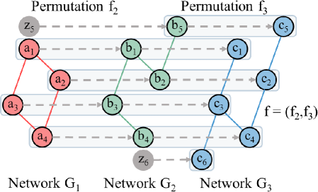
Figure 1: An example of how an MNA of three networks is represented using two permutations. Networks $G_{1}(V_{1},E_{1}),G_{2}(V_{2},E_{2})$, and $G_{3}(V_{3},E_{3})$ are ordered in terms of the number of nodes from the smallest to the largest one. Since $\lvert V_{2}\rvert=5$ and $\lvert V_{3}\rvert=6$, $f_{2}$ and $f_{3}$ are permutations of size 5 and 6, respectively. (Here, nodes $z_{5}$ and $z_{6}$ are dummy nodes added to $V_{1}$ and $V_{2}$, respectively, intended to enforce the $m=n$ constraint described in the text, i.e., to ensure that $\lvert{\bar{V}_{1}}\rvert=\lvert V_{2}\rvert=5$ and $\lvert{\bar{V}_{2}}\rvert=\lvert V_{3}\rvert=6$; Section S2.1.1). The permutations create disjoint clusters in this toy example that cover all the nodes in the networks. For example, the cluster created through the mapping $a_{1}\mapsto b_{1}\mapsto c_{1}$ is $(\{a_{1}\},\{b_{1}\},\{c_{1}\})$, and the cluster created through the mapping $b_{5}\mapsto c_{5}$ is $(\varnothing,\{b_{5}\},\{c_{5}\})$.

2.1.3 Crossover function

The core of a GA is the crossover function, which creates a child alignment from two parent alignments (Bäck, 1996). A crossover function such that the child alignment has characteristics of both parents results in better GA performance. MAGNA++ made use of a novel crossover function for PNA, which used the concept of a Cayley graph to create a child permutation (see below). Here, we extend MAGNA++’s crossover function by formulating a notion of a Cayley graph for MNA.

First, we describe MAGNA++’s crossover function using its notion of a Cayley graph in the context of PNA. Recall that we can represent a PNA of $G_{1}$ to $G_{2}$ using a permutation $f$ of size $n$. Let $S_{n}$ denote the set of all permutations of size $n$. A transposition of a permutation is a new permutation that fixes every element of the original permutation except two elements, which are swapped. The transposition of a permutation and the original permutation are of similar alignment quality since a small perturbation of a permutation is not expected to greatly affect alignment quality. Thus, in order to design a crossover function, a graph can be created whose topology takes advantage of the fact that a transposition of a permutation does not greatly affect its alignment quality. MAGNA++ constructs such a graph so that its node set is $S_{n}$ and so that there is an edge between nodes $f\in S_{n}$ and $g\in S_{n}$ if and only if there is a transposition $\nu$ such that $f=\nu g$, i.e. if and only if the permutations $f$ and $g$ differ by a transposition. The resulting graph is the PNA-based Cayley graph. This graph has the desired property that, given permutations $f$ and $g$, the child permutation $f\otimes g$ will be the midpoint of the geodesic (shortest) path between $f$ and $g$, and as such, it is expected to share approximately half of its aligned pairs with each of $f$ and $g$ (Saraph and Milenković, 2014).

Second, we define our crossover function using the formulation of the Cayley graph in the context of MNA. Let $n_{l}=\lvert V_{l}\rvert$ for $l=1,\ldots,k$ and let $S_{n_{l}}$ denote the set of all permutations of size $n_{l}$. Recall that we can represent an MNA of $k$ networks using a multi-permutation $f=(f_{2},f_{3},\ldots,f_{k})$ containing permutations of sizes $n_{2},n_{3},\ldots,n_{k},$ respectively. Thus, $S=S_{n_{2}}\times S_{n_{3}}\times\ldots\times S_{n_{k}}$ is the set of all multi-permutations (i.e., MNAs) of the $k$ networks. Analogous to the PNA-based Cayley graph above, we can create a graph whose topology takes advantage of the fact that a transposition of a single permutation in a multi-permutation does not greatly affect its alignment quality. We construct such a graph so that its node set is $S$ and so that there is an edge between $(f_{2},\ldots,f_{k})\in S$ and $(g_{2},\ldots,g_{k})\in S$ if and only if there is a transposition $\nu$ such that $f_{l^{\prime}}=\nu g_{l^{\prime}}$ for some $l^{\prime}\in\{2,\ldots,k\}$ and $f_{l}=g_{l}$ for $l\neq l^{\prime}$, i.e., if and only if only one pair of permutations in the two multi-permutations differs only by a transposition. The resulting graph is the MNA-based Cayley graph. This graph allows us to design a crossover function as follows. Given multi-permutations $f\in S$ and $g\in S$, let $f\otimes g$ be the midpoint of the geodesic path between $f$ and $g$. The permutations in a multi-permutation are independent of each other in the sense that changing one permutation does not affect another permutation. So, $f\otimes g=(f_{2}\otimes g_{2},f_{3}\otimes g_{3},\ldots,f_{k}\otimes g_{k})$, where $f_{l}\otimes g_{l}$ is MAGNA++’s crossover function for two permutations. $f\otimes g$ will share characteristics with both $f$ and $g$ since each permutation $f_{l}\otimes g_{l}$ in the multi-permutation $f\otimes g$ will have characteristics of both permutations $f_{l}$ and $g_{l}$ for $l=1,\ldots,k$. Thus, if we let the midpoint $f\otimes g$ be the crossover, then we can expect that the child MNA shares characteristics of each of the two parent MNAs.

2.1.4 Fitness function

The fitness function that multiMAGNA++ directly optimizes is a combined measure of both edge and node conservation that we define below. We optimize this combined measure intentionally, because we aim to find out whether directly optimizing edge conservation in addition to node conservation would result in superior alignments when compared to the existing methods, most of which optimize node conservation only (but then they evaluate the resulting alignments based on their edge conservation; Section 1). The alignment quality measure that we use is a convex combination of an edge conservation measure, $S_{E}$, and a node conservation measure, $S_{N}$: $\alpha S_{E}+(1-\alpha)S_{N}$. The $\alpha$ parameter varies from $0$ to $1$ and controls for the influence of edge vs. node conservation. The edge and node conservation measures that we use are as follows.

The edge conservation measure that we use is conserved interaction quality (CIQ) (Alkan and Erten, 2014). CIQ is a weighted sum of edge conservation between all pairs of aligned clusters. It is a generalization of the established S³ (Saraph and Milenković, 2014) edge conservation measure from PNA to MNA. CIQ is calculated as follows. Given clusters $a$ and $b$, let $\lvert E_{a,b}\rvert$ be the number of edges that connect the clusters. Let $r(a,b)$ be the number of networks that the edges which connect the clusters belong to. Let $s(a,b)$ be the number of networks that contain at least one node in both clusters. Let the edge conservation between two clusters be $cs(a,b)$, where either (i) $cs(a,b)=0\mbox{ if }r(a,b)\leq 1$ or (ii) $cs(a,b)=\frac{r(a,b)}{s(a,b)}\mbox{ otherwise}$. That is, $cs(a,b)$ is 0 if no edges connect the two clusters or if the edges that connect the clusters belong to only one network. Otherwise, $cs(a,b)$ is the fraction of networks that the edges connecting the two clusters belong to. Given edge conservation between all pairs of clusters, total edge conservation is $S_{E}=\mbox{CIQ}=\frac{\sum_{a,b}\lvert E_{a,b}\rvert cs(a,b)}{\sum_{a,b}\lvert E_{a,b}\rvert}$.

The node conservation measure that we use is an MNA quality measure that we propose as our contribution. Node conservation refers to internal cluster quality, meaning that in a good alignment, nodes in each cluster should be highly similar to each other with respect to some node cost function – see below). We measure a cluster’s internal quality as mean node similarity across all node pairs in the cluster. To account for all clusters, we take the mean of the above measure across all clusters. Formally, let $s(u,v)$ be the similarity between nodes $u$ and $v$ with respect to some node cost function (we discuss below the specific node cost functions that we use). Then, given the aligned clusters $a_{i}$, $i=1,\ldots,n$, the node conservation measure is $S_{N}=\frac{1}{n}\sum_{i=1}^{n}{\frac{1}{{\lvert a_{i}\rvert\choose 2}}\sum_{(u,v)\in\mathcal{P}(a_{i})}s(u,v)},$ where $\lvert a_{i}\rvert$ is the size of $a_{i}$, and $\mathcal{P}(a_{i})$ is the set of all pairs of nodes in $a_{i}$. Since multiMAGNA++ maximizes a convex combination of edge and node conservation measures, the values of $S_{N}$ should ideally be in the same range as the values of $S_{E}$. Given that CIQ score lies between 0 to 1, in order to let $S_{N}$ also lie in that range, each $s(u,v)$ needs to lie between 0 and 1. MultiMAGNA++, like MAGNA++, allows for using any kind of node cost function to compute node conservation.

An NA method can use network topology alone in the alignment construction process, or it can also include biological information external to network topology, such as sequence information, while constructing alignments. We study the effect on alignment quality when constructing alignments using only network topology versus also including sequence information. When constructing topology-only alignments, we let multiMAGNA++ optimize a combination of CIQ (corresponding to edge conservation $S_{E}$) and graphlet degree vector similarity (GDVS) (corresponding to $s(u,v)$ that is needed to compute node conservation $S_{N}$), where GDVS is a sensitive measure of topological similarity of extended neighborhoods of two nodes (Milenković and Pržulj, 2008). To combine $S_{E}$ and $S_{N}$, we use $\alpha=0.5$, to give equal contribution to edge conservation and node conservation. When constructing topology+sequence alignments, we let multiMAGNA++ optimize a convex combination of: 1) the fitness function that we optimize for topology-only alignments (i.e., $0.5\times\mbox{CIQ}+0.5\times\mbox{GDVS}$) and 2) BLAST sequence similarity as captured by E-value (Ye et al., 2006), as follows: $0.5\times(0.5\times\mbox{CIQ}+0.5\times\mbox{GDVS})+0.5\times\mbox{E-value}$, where E-value is a commonly used node cost function for protein similarity (Liao et al., 2009; Alkan and Erten, 2014; Gligorijević et al., 2015). This way, when constructing topology+sequence alignments, we give equal contribution to the topological part (i.e., CIQ and GDVS combined) and the sequence part (i.e., E-value) of the fitness function. Here, GDVS already lies in the [0,1] range, as required, but E-value does not. So, we convert E-value into a measure of similarity that lies between 0 and 1 (Section B.1.2), before we combine this measure with GDVS.

2.1.5 Tying the GA together

We have discussed the components of our multiMAGNA++ that are needed to optimize the above fitness function using a population of MNAs. Additional parameters are: 1) how to generate the initial population; 2) which population size to use; 3) how to choose which individuals of the population to cross; and 4) how many generations to run the algorithm for. For our choices of these parameters’ values, see Section B.1.3; we rely on our comprehensive evaluation of the optimal parameter values conducted in our previous MAGNA++ work.

2.1.6 Running time and complexity

MAGNA++ and multiMAGNA++ evolve a population of $p$ alignments over $N$ generations. For every generation, the methods perform two significant computations: (1) alignment quality for $p$ alignments with respect to both node and edge conservation, and (2) crossover of $O(p)$ pairs of parent alignments. Given two networks $G_{1}(V_{1},E_{1})$ and $G_{2}(V_{2},E_{2})$, where $|V_{1}|\leq|V_{2}|$, MAGNA++ has a time complexity of $O(Np|V_{2}|+Np(|E_{1}|+|E_{2}|))$, since computing node conservation takes $O(|V_{2}|)$, computing edge conservation takes $O(|E_{1}|+|E_{2}|)$, and computing crossover takes $O(|V_{2}|)$. MAGNA++ improved upon the time complexity of MAGNA (Vijayan et al., 2015), and MAGNA improved upon the complexity of existing (PNA) methods (Saraph and Milenković, 2014). Hence, it is likely that multiMAGNA++ will be faster than existing MNA methods, most of which are also MNA-equivalents of their PNA versions, just as multiMAGNA++ is an MNA-equivalent of MAGNA++. In particular, let $G_{1}(V_{1},E_{1}),\ldots,G_{k}(V_{k},E_{k})$ be $k$ networks ordered by size as above, where $|E|=\sum_{l=1}^{k}|E_{l}|$. Then, the time complexity of multiMAGNA++ is $O(Npk|V_{k}|+Np|E|)$, since computing node conservation takes $O(k|V_{k}|)$, computing edge conservation takes $O(|E|)$, and computing crossover takes $O(k|V_{k}|)$. Clearly, the time complexity of multiMAGNA++ scales linearly with the total number of nodes and edges. Also, unlike with the existing MNA methods, the complexity of multiMAGNA++ scales linearly (rather than exponentially in, for example, GEDEVO-M’s case) with the number of networks. Importantly, since calculating alignment quality tends to be a bottleneck for multiMAGNA++, and since alignment quality can be calculated independently for each alignment, we parallelize this calculation in order to achieve a further speedup. For multiMAGNA++, this results in speedup that is almost linear in terms of the number of CPU cores used.

2.2 Evaluation

2.2.1 Dataset

We use five PPI network sets: a network set with known true node mapping and four network sets with unknown node mapping.

Networks with known node mapping. This network set, Yeast+%LC, has been used by many existing studies (Kuchaiev et al., 2010; Milenković et al., 2010; Kuchaiev and Pržulj, 2011; Patro and Kingsford, 2012; Saraph and Milenković, 2014). It contains a high-confidence S. cerevisiae (yeast) PPI network with 1,004 proteins and 8,323 PPIs (Collins et al., 2007), along with five yeast lower-confidence networks that add PPIs of decreasing confidence to the high-confidence network. We align all six networks at once. We know the true node mapping since the networks contain the same nodes. Thus, we can evaluate how accurately each MNA method reconstructs this mapping (Section 2.2.3).

Networks with unknown node mapping. The four network sets with unknown node mapping are PHY1, PHY2, Y2H1 and Y2H2 (Meng et al., 2015). Each network set contains PPI data of four species, S. cerevisiae (yeast/Y), D. melanogaster (fly/F), C. elegans (worm/W), and H. sapiens (human/H), obtained from BioGRID (Breitkreutz et al., 2008) in November 2014. The networks in the four sets were extracted based on the following interaction types and confidence levels of the PPIs: (i) all physical PPIs supported by at least one publication (PHY1), (ii) all physical PPIs supported by at least two publications (PHY2), (iii) only yeast two-hybrid physical PPIs supported by at least one publication (Y2H1), and (iv) only yeast two-hybrid physical PPIs supported by at least two publications (Y2H2). Just as in our recent work (Meng et al., 2015), we use network sets with different PPI types (all physical vs. only yeast two-hybrid) to test the robustness of our approach to the choice of PPI data type. We use network sets with PPIs supported by at least two publications since those PPIs are believed to be more reliable than PPIs supported by only one publication (Cusick et al., 2009). For each of the networks, we use only its largest connected component (Table A3). The largest connected component of the fly and worm networks in the PHY2 and Y2H2 sets are too small (53-331 nodes) for analyses. Thus, we remove the fly and worm networks from both PHY2 and Y2H2, resulting in each of the two sets containing only two networks. Since we cannot measure how accurately the aligners reconstruct the true node mapping when aligning networks with unknown node mapping, we use alternative alignment accuracy measures (Section 2.2.4).

Some of these alternative measures rely on Gene Ontology (GO) annotations of proteins (The Gene Ontology Consortium, 2000). We use GO data obtained from the Gene Ontology database in January 2016. We use only GO annotations that were obtained experimentally.

2.2.2 Existing methods we evaluate against

The methods we evaluate against are all existing MNA methods for which the code is available and could be run without errors. Namely, we comprehensively evaluate against: i) IsoRankN (Liao et al., 2009), ii) MI-Iso (Faisal et al., 2014), iii) GEDEVO-M (Ibragimov et al., 2014), iv) BEAMS (Alkan and Erten, 2014), and FUSE (Gligorijević et al., 2015). Also, we evaluate our approach and each of the existing approaches against their corresponding random MNA counterparts, to ensure statistical significance of each result (see below). We tried to evaluate against SMETANA (Sahraeian and Yoon, 2013), but were unable to do so due to SMETANA’s high memory usage and high runtime on the larger network sets. Similarly, we tried to evaluate against NetCoffee (Hu et al., 2014), but we were unable to do so on our machines, because of incompatibility of NetCoffee’s library dependencies. Finally, we do not evaluate against the remaining existing method, CSRW (Jeong and Yoon, 2015), since its publication does not make available the code for this method.

To fairly evaluate the methods, we study the effect on alignment quality of (i) using only network topology while constructing alignments (resulting in topology-only alignments) versus (ii) also including sequence information into the alignment construction process (resulting in topology+sequence alignments). For topology-only alignments, we set method parameters to ignore any sequence information (Table A4). All methods except BEAMS and FUSE can be run in the topology-only mode. For topology+sequence alignments, we set method parameters to include BLAST sequence information (Section 2.1.4 and Table A4). All methods but GEDEVO-M can be run in the topology+sequence mode.

The MNA methods that we evaluate are classified into one-to-one (1-1) and many-to-many (m-m) aligners. Of the methods, GEDEVO-M, FUSE, and multiMAGNA++ are 1-1 aligners while IsoRankN, MI-Iso, and BEAMS are m-m aligners. Since 1-1 and m-m aligners result in different outputs, meaning that the aligned clusters produced by 1-1 aligners contain at most one node from each network while m-m aligners have no such restriction, it is more fair to compare 1-1 aligners with other 1-1 aligners, and m-m aligners with other m-m aligners. Comparison of 1-1 aligners with m-m aligners needs to be taken with caution due to their different output types. Yet, we include such comparison, since only two of the existing methods (GEDEVO-M and FUSE) are 1-1, i.e., is of the same type as our proposed multiMAGNA++ approach, and we want to include more MNA approaches into the comparison to properly demonstrate the superiority of our approach.

To allow for as fair as possible comparison of 1-1 and m-m aligners, we compute the statistical significance of each approach’s alignment quality score, in order to compare the resulting $p$-values between the different MNA approaches instead of (or at least in addition to) comparing the approaches’ raw alignment quality scores. Namely, for each approach and each of its alignments (depending on the input networks), we construct a set of 10,000 corresponding random alignments (10,000 is what was practically possible given the relatively large running time of computing the functional alignment quality scores), under a null model that accounts for characteristics of both the given approach and the input networks. That is, each random alignment conserves the number of clusters and the cluster size distribution of the corresponding actual alignment. Then, we compute the $p$-value of the given alignment quality score as the frequency of obtaining equal or better score among the 10,000 random alignments. This way, by comparing $p$-values of the different approaches instead of (or in addition to, in case $p$-values of the different approaches are tied) the approaches’ raw scores, where the $p$-values account for the null model of each approach, we are aiming to account for the differences between output types of 1-1 and m-m MNA approaches, in order to allow for their more fair comparison. We consider an alignment score to be significant if its $p$-value is less than 0.001. Note that we obtain qualitatively identical results when we use a more flexible $p$-value threshold of 0.01.

2.2.3 Topological alignment quality measures

We propose three new measures of topological alignment quality for MNA, as described below. Whenever we calculate alignment quality (here or in Section 2.2.4), we only consider aligned clusters with at least two nodes, unless specified otherwise.

Adjusted node correctness (NCV-MNC). A good MNA approach should find aligned clusters that are internally consistent with respect to protein labels. For networks with known node mapping, labels correspond to protein names. In this case, we use an existing notion of node correctness (MNC, defined below) to measure internal cluster consistency, and we consider this to be a topological alignment quality measure. First, we use an existing notion of normalized entropy (NE) to measure how likely it is to observe in a given cluster, at random, the same or higher level of internal consistency with respect to protein names. Given cluster $c$, $\textrm{NE}(c)=-\frac{1}{\log d}\sum_{i=1}^{d}{p_{i}\log p_{i}}$, where $d$ is the number of unique protein names in $c$, and $p_{i}$ is the fraction of nodes in $c$ with protein name $i$. The lower the NE, the more consistent the cluster. Then, we let MNC be one minus the mean of NEs across all clusters in the alignment. For networks with unknown node mapping, protein labels correspond to their GO terms. In this case, since GO terms capture proteins’ functional information, we consider the corresponding measure of internal cluster consistency to be a functional alignment quality measure, and we describe this measure in more detail in Section 2.2.4.

A good MNA approach should also align (or cover) many of the proteins from the aligned networks. So, we combine the above notion of cluster consistency (i.e. MNC) with an existing notion of node coverage (NCV, defined below) into a new measure that we call adjusted node correctness. NCV is the fraction of all nodes that are part of the alignment (i.e., of the aligned clusters with two or more nodes) out of all nodes in the networks. Then, we define adjusted node correctness as: $\textrm{NCV-MNC}=\sqrt{(\textrm{NCV})(\textrm{MNC})}$. This geometric mean penalizes alignments that have a low alignment quality score with respect to at least one of NCV or MNC.

Adjusted cluster interaction quality (NCV-CIQ). Further, a good MNA approach should find a large amount of network structure that is common to many (ideally all) of the aligned networks, which is typically referred to as edge conservation. Here, we rely on the existing CIQ measure, which we have already defined in Section 2.1.4. CIQ can be seen as a generalization of the established S³ (Saraph and Milenković, 2014) edge conservation measure from PNA to MNA. Just as above, since we want the conserved edges to cover many nodes, we combine CIQ with NCV into a new measure, adjusted cluster interaction quality, as follows: $\textrm{NCV-CIQ}=\sqrt{(\textrm{NCV})(\textrm{CIQ})}$.

Largest common connected subgraph (LCCS). Finally, a good MNA approach should group the aligned edges to form connected and dense network regions (as opposed to the aligned edges being isolated in a random manner). To capture this, we rely on an established notion of the size of LCCS, but we propose a novel generalization of this notion from PNA to MNA. The details of this novel LCCS measure are as follows.

Given an MNA of $k$ networks $G_{1}(V_{1},E_{1})$, $G_{2}(V_{2},E_{2})$, $\ldots$, $G_{k}(V_{k},E_{k})$, we define the fully conserved common subgraph as the graph in which each aligned cluster is fused into a supernode and there is an edge between two supernodes if and only if there is an edge belonging to each of the $k$ networks that connects the two aligned clusters. Then, the LCCS is the largest connected component of the fully conserved common subgraph. To measure the quality of the LCCS of the given alignment by simultaneously accounting for the LCCS’s number of nodes as well as its number of edges, we extend the PNA-based LCCS measure introduced in (Saraph and Milenković, 2014) to MNA. Let $n$ be the number of nodes in the LCCS and $n_{max}=\min\{|V_{1}|,\ldots,|V_{k}|\}$ be the maximum possible number of nodes in the LCCS. Let $e$ be the number of edges in the LCCS and $e_{max}=\min\{|E_{1}(\textrm{LCCS})|,\ldots,|E_{k}(\textrm{LCCS})|\}$ be the maximum possible number of edges in the LCCS, where $E_{l}(\textrm{LCCS})$ is the set of edges induced by the network nodes in the LCCS on network $G_{l}$. Then, $\textrm{LCCS}=\sqrt{\frac{n}{n_{max}}\frac{e}{e_{max}}}$; this score is high when the LCCS both has many nodes and is dense.

2.2.4 Functional alignment quality measures

We use three existing measures of functional alignment quality for MNA, modifying in the process some measures to allow for MNA instead of just PNA, as described below. These measures rely on GO data. Since many GO annotations are obtained via sequence analyses, and since we also use sequence information in the alignment construction process, to avoid a circular argument, we only use GO annotations that have been obtained experimentally.

Mean Normalized Entropy (MNE). Recall from Section 2.2.3 that a good MNA should have clusters that are internally consistent. When the true node mapping is unknown, we use GO terms to measure internal consistency. For this purpose, we use the same NE measure as in Section 2.2.3, where now $d$ is the number of unique GO terms, and $p_{i}$ is the ratio of the number of proteins annotated with GO term $i$ to the total number of protein-GO term annotations (independent of the GO term) in the cluster. The lower the NE, the more consistent the cluster is with respect to the GO terms. We measure the internal consistency over all clusters using MNE, the mean of the NEs across all clusters in the alignment (Liao et al., 2009).

GO correctness (GC). We extend the existing notion of GO correctness from PNA to MNA as another measure of internal cluster consistency (Kuchaiev et al., 2010). GO correctness measures the extent to which pairs of proteins that are aligned together are annotated with the same GO term(s). For MNA, we consider two proteins to be aligned together if they are in the same cluster. Formally, to calculate GC, we first transform an MNA consisting of aligned node clusters into a list of aligned node pairs. This is done by populating this list with all pairs of proteins that are in the same aligned cluster. Then, we filter this list to keep only pairs in which each of the two proteins has at least one GO term. Given the resulting filtered list, GC is the fraction of the filtered protein pairs in which the two proteins share at least one GO term. In this analysis, we ignore GO terms that are associated with only one protein in the MNA.

Accuracy of protein function prediction. We extend the protein function prediction approach by Meng et al. (2015) from PNA to MNA. In a leave-one-out-cross-validation-like manner, we measure how well we can predict function (i.e., GO term) of a given protein based on the protein’s aligned partner when we hide the protein’s functional information, repeating this for each currently annotated protein from the above filtered list of aligned protein pairs and each of its GO terms. Then, given all predicted protein-GO term prediction associations, we calculate accuracy of the predictions via precision, recall, and F-score measures. Formally, let $X$ be the set of predicted protein-GO term associations, and let $Y$ be the set of true protein-GO term associations. Then, the precision of protein function prediction is: P-PF $=\frac{\lvert X\cap Y\rvert}{\lvert X\rvert}$. The recall is: R-PF $=\frac{\lvert X\cap Y\rvert}{\lvert Y\rvert}$. The F-score, F-PF, is the harmonic mean of precision and recall. In this analysis, we ignore GO terms that are associated with only one protein in the MNA.

3 Results and Discussion

We compare multiMAGNA++ (Section 2.1) to five existing MNA methods (IsoRankN, MI-Iso, GEDEVO-M, BEAMS, FUSE; Section 2.2.2) on a network set with known node mapping, Yeast+%LC, and four network sets with unknown node mapping, PHY1, PHY2, Y2H1, and Y2H2 (Section 2.2.1). We measure alignment quality using both topological and functional alignment quality measures (Sections 2.2.3 and 2.2.4). We measure the statistical significance of each result (Section 2.2.2).

Recall that we consider topology-only alignments as well as topology+sequence alignments (Section 2.2.2). For each data set and alignment quality measure, since we want to give each method the best case advantage, we do the following. Henceforth, when we report results for the given method, we do so for the best of its topology-only alignment and its topology+sequence alignment, unless otherwise noted. Note that even if we restrict our method evaluation only to topology-only alignments, or only to topology+sequence alignments, the results are qualitatively similar, and all detailed results are reported in the Supplement.

3.1 Method comparison in terms of accuracy

3.1.1 Network set with known node mapping

	Topological measures			Functional measures
Method	NCV-MNC	NCV-CIQ	LCCS	MNE	GC	F-score
MI-Iso	0.5638 p $<$ 1e-4	0.7908 p $<$ 1e-4	0.2508 p $<$ 1e-4	0.9508 p $<$ 1e-4	0.6137 p $<$ 1e-4	0.4709 p $<$ 1e-4
IsoRankN	0.8967 p $<$ 1e-4	0.9219 p $<$ 1e-4	0.8929 p $<$ 1e-4	0.9532 p $<$ 1e-4	0.9748 p $<$ 1e-4	0.9367 p $<$ 1e-4
BEAMS	0.8215 p $<$ 1e-4	0.8342 p $<$ 1e-4	0.7827 p $<$ 1e-4	0.9667 p $<$ 1e-4	0.9882 p $<$ 1e-4	0.8625 p $<$ 1e-4
FUSE	0.6299 p $<$ 1e-4	0.6943 p $<$ 1e-4	0.5123 p $<$ 1e-4	0.9618 p $<$ 1e-4	0.7744 p $<$ 1e-4	0.5953 p $<$ 1e-4
GEDEVO-M	0.2969 p $<$ 1e-4	0.8574 p $<$ 1e-4	0.4104 p $<$ 1e-4	0.9610 p $<$ 1e-4	0.4333 p $<$ 1e-4	0.1586 p $<$ 1e-4
multiMAGNA++	0.9241 p $<$ 1e-4	0.9574 p $<$ 1e-4	0.9201 p $<$ 1e-4	0.9341 p $<$ 1e-4	0.9897 p $<$ 1e-4	0.9392 p $<$ 1e-4

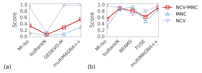
Figure A5: NCV-MNC, NCV, and MNC for the Yeast+%LC network set for (a) topology-only alignments and (b) topology+sequence alignments.

Table 1: Alignment accuracy of different MNA approaches for the Yeast+%LC network set in terms of topological NCV-MNC, NCV-CIQ, and LCCS measures and functional MNE, GO correctness (GC), and F-score measures. The symbol “p” signifies $p$-values of the observed alignment scores. For each alignment quality measure, and for each network set, the best method (i.e., the method with the lowest $p$-value, or the method with the best alignment quality score if the $p$-values are tied) is bolded. The alignment scores that are not statistically significant, if any, are greyed out and italicized. Note that for MNE, the lower the score, the better the alignment quality. For all other measures, the higher the score, the better the alignment quality. For equivalent results broken down by topology-only alignments and by topology+sequence alignments, see Tables A5-A6 and Figures A5-A8.

While on this data all methods produce statistically significant alignments with respect to all alignment quality measures, multiMAGNA++ outperforms all existing methods with respect to all topological and functional alignment quality measures (Table 1). Furthermore, only multiMAGNA++, IsoRankN, and BEAMS perform well consistently for each of the measures. Note that GEDEVO-M, which optimizes edge conservation like multiMAGNA++, does not perform as well as the other methods. (In the original GEDEVO-M publication (Ibragimov et al., 2014), nearly perfect alignments of the networks with known node mapping were reported with respect to node conservation. We found that this is because GEDEVO-M’s implementation uses the lexicographic ordering of the node names. After we remove this bias by renaming the node names to randomly generated strings, the accuracy of GEDEVO-M drops, as reported in our results.) The inferior behavior of GEDEVO-M compared to the other methods could be because GEDEVO-M can use only topological information when constructing alignments, while all other methods can use both topological and sequence information. Namely, Yeast+%LC, comprising six networks that all have the same set of nodes, contains many inter-network pairs of nodes that are the same proteins (this does not happen in networks with unknown node mapping that have different node sets). For such pairs, sequence similarity scores are significantly higher than for any other pairs of nodes. These inter-network node pairs can potentially form aligned clusters that have very high intra-cluster sequence similarity due to the node pairs being the same protein. This may be the main reason why on Yeast+%LC, the MNA approaches perform much better for topology+sequence alignments compared to topology-only alignments (Tables A5 and A6). This is not the case for the network sets with unknown node mapping, PHY1, PHY2, Y2H1, and Y2H2, as we see in the following section.

3.1.2 Networks with unknown node mapping

		Topological measures		Functional measures
	Method	NCV-CIQ	LCCS	MNE	GC	F-score
PHY1	MI-Iso	0.2517 p $<$ 1e-4	0.0000 p = 1.000	0.8224 p $<$ 1e-4	0.2732 p $<$ 1e-4	0.0492 p $<$ 1e-4
	IsoRankN	0.1012 p $<$ 1e-4	0.0258 p $<$ 1e-4	0.7977 p $<$1e-4	0.3279 p $<$1e-4	0.0838 p $<$1e-4
	BEAMS	0.3250 p $<$ 1e-4	0.0000 p = 1.000	0.8944 p = 0.895	0.4084 p = 1.000	0.0457 p $<$ 1e-4
	FUSE	0.0679 p = 5e-4	0.0000 p = 1.000	0.8781 p $<$ 1e-4	0.2268 p $<$ 1e-4	0.0472 p $<$ 1e-4
	GEDEVO-M	0.3554 p $<$ 1e-4	0.1613 p $<$1e-4	0.9205 p = 1.000	0.1721 p $<$ 1e-4	0.0324 p $<$ 1e-4
	multiMAGNA++	0.4046 p $<$1e-4	0.1064 p $<$ 1e-4	0.8449 p $<$ 1e-4	0.1759 p $<$ 1e-4	0.0353 p $<$ 1e-4
Y2H1	MI-Iso	0.1935 p $<$ 1e-4	0.0264 p $<$ 1e-4	0.8992 p = 0.396	0.2092 p $<$ 1e-4	0.0382 p $<$ 1e-4
	IsoRankN	0.1315 p $<$ 1e-4	0.0264 p $<$ 1e-4	0.8447 p $<$1e-4	0.3247 p $<$ 1e-4	0.0822 p $<$ 1e-4
	BEAMS	0.2856 p $<$ 1e-4	0.0000 p = 1.000	0.9159 p = 0.363	0.3945 p $<$1e-4	0.0856 p $<$1e-4
	FUSE	0.0480 p $<$ 1e-4	0.0000 p = 1.000	0.8781 p $<$ 1e-4	0.2369 p $<$ 1e-4	0.0483 p $<$ 1e-4
	GEDEVO-M	0.4511 p $<$ 1e-4	0.0722 p $<$ 1e-4	0.9032 p = 0.919	0.1879 p = 6e-4	0.0347 p $<$ 1e-4
	multiMAGNA++	0.4943 p $<$1e-4	0.1088 p $<$1e-4	0.8899 p = 6e-4	0.2040 p $<$ 1e-4	0.0428 p $<$ 1e-4

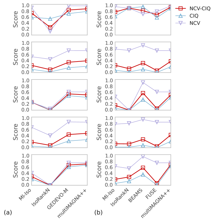
Figure A6: NCV-CIQ, NCV, and CIQ for the five network sets (Yeast+%LC, PHY1, PHY2, Y2H1, and Y2H2 from top to bottom) for (a) topology-only alignments and (b) topology+sequence alignments.

Table 2: Alignment accuracy of different MNA approaches for the PHY1 and Y2H1 network sets in terms of topological NCV-CIQ and LCCS measures and functional MNE, GO correctness (GC), and F-score measures. The symbol “p” signifies $p$-values of the observed alignment scores. For each alignment quality measure, and for each network set, the best method (i.e., the method with the lowest $p$-value, or the method with the best alignment quality score if the $p$-values are tied) is bolded. The alignment scores that are not statistically significant, if any, are greyed out and italicized. Note that for MNE, the lower the score, the better the alignment quality. For all other measures, the higher the score, the better the alignment quality. Equivalent results for the remaining networks with unknown true node mapping (PHY2 and Y2H2) are shown in Table A7. For equivalent results broken down by topology-only alignments and by topology+sequence alignments, see Tables A8-A9 and Figures A6-A8.

Over all four network sets with unknown node mapping and all five alignment quality measures, multiMAGNA++ produces the most of statistically significant alignments. Namely, in only one of the $4\times 5=20$ cases, its alignment is non-significant, while the existing methods have non-significant alignments in four to eight of the 20 cases (Table 2 and Table A7). This has important implications for predicting any new biological knowledge from a given method’s alignment, since an alignment is practically meaningful only if it is statistically significant.

In terms of topological alignment quality, multiMAGNA++ is superior to MI-Iso, IsoRankN, and FUSE in all cases, and it is also superior to BEAMS and GEDEVO-M in 75% of all cases (Table 2 and Table A7).

In terms of functional alignment quality, multiMAGNA++ is overall comparable to all methods, with the exception of IsoRankN, which is the best performing method in most of the cases. However, IsoRankN’s performance is data-specific, as it works great for some network sets but completely fails for others (such as PHY2; Table A7), while multiMAGNA++ performs consistently well on all network sets.

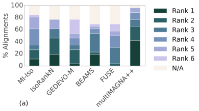
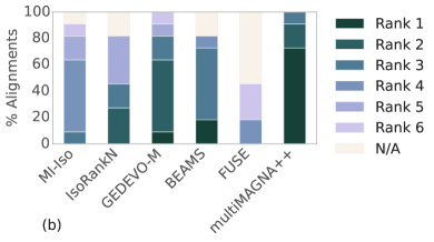
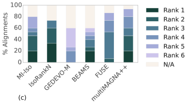
Figure 2: Ranking of the MNA methods across all of Yeast+%LC, PHY1, PHY2, Y2H1, and Y2H2 network sets with respect to (a) all measures, (b) topological NCV-MNC, NCV-CIQ, and LCCS measures, and (c) functional MNE, GC, and F-score measures. The ranking of each method is expressed as a percentage of all evaluation tests in which the given method is the best performing (“Rank 1”), the second best performing (“Rank 2”), etc. aligner of all considered methods. By “best”, we mean the method with the lowest $p$-value, or the method with the best alignment quality score if the $p$-values are tied. If an alignment score of a method is not statistically significant, the method is not ranked and is labelled as “N/A”. For equivalent results broken down by topology-only alignments and by topology+sequence alignments, see Figure A9.

3.1.3 Summary

We summarize our results over all network sets and all alignment quality measures to identify the overall ranking of the different MNA methods, i.e., to identify the best (rank 1), second best (rank 2), third best (rank 3), etc. performing of all methods. MultiMAGNA++ has barely any non-significant alignments (3.9% of all cases), while the existing methods have 15.4%–30.8% non-significant alignments (Figure 2(a)). This makes multiMAGNA++ the best method in this context. Further, multiMAGNA++ is superior to all other methods (rank 1) in more cases than any other method (Figure 2(a)). Importantly, only multiMAGNA++ and BEAMS are superior to all existing methods (i.e., have rank 1) in terms of both topological (Figure 2(b)) and functional (Figure 2(c)) alignment quality; all other methods have rank 1 with respect to at most one of topological and functional quality. In this context, multiMAGNA++ and BEAMS are outperforming the other methods, while at the same time, multiMAGNA++ beats BEAMS, especially in terms of topological alignment quality.

In conclusion, when comparing the different methods in terms of alignment accuracy, multiMAGNA++ drastically beats the existing methods with respect to topological alignment quality (Figure 2(b)), and it is comparable to the existing methods with respect to functional alignment quality (Figure 2(c)).

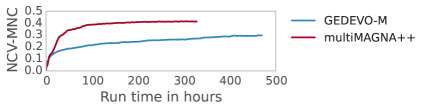
Figure 3: NCV-MNC as a function of the number of hours spent by multiMAGNA++ and GEDEVO-M when using a single thread, for topology-only alignments of Yeast+%LC networks. Both multiMAGNA++ and GEDEVO-M are run for 100,000 generations. These are representative results. For equivalent results for the other measures and for the networks with unknown node mapping, see Figures A10 and A11.

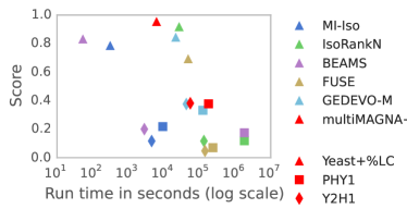
Figure 4: NCV-CIQ as a function of time when using 64 threads for the three network sets with more than two networks (we leave out these results for PHY2 and Y2H2 that have two networks each; Section 2.2.1). These are representative results. For equivalent results for the remaining measures, as well as for using a single thread, see Figures A12-A14.

3.2 Method comparison in terms of time complexity

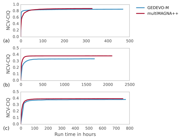
Figure A10: NCV-CIQ as a function of the number of hours spent by multiMAGNA++ and GEDEVO-M when using a single thread, for topology-only alignments of (a) Yeast+%LC, (b) PHY1, and (c) Y2H1 network sets. We only show these results for the three network sets with more than two networks; we leave out these results for PHY2 and Y2H2 that have two networks each. Both multiMAGNA++ and GEDEVO-M are run for 100,000 generations.

First, we compare multiMAGNA++ with GEDEVO-M, as these methods are the most similar since they are both evolutionary algorithms. This allows us to observe their behavior over time to see how fast they converge to a solution. When we run both multiMAGNA++ and GEDEVO-M for 100,000 generations, we observe the following (Figure 3 and Figures A10 and A11). In general, GEDEVO-M converges slower than multiMAGNA++. In fact, GEDEVO-M often does not converge even after 100,000 generations (Figure 3). Thus, multiMAGNA++ can be stopped much earlier than GEDEVO-M, while in the process mostly leading to superior alignment quality. On top of this, the time complexity of GEDEVO-M is exponential with respect to the number of networks to be aligned as opposed to the linear time complexity for multiMAGNA++ (Section 2.1.6).

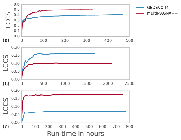
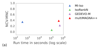
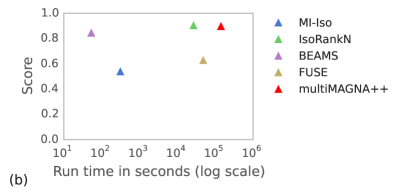
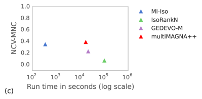
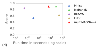
Figure A11: LCCS as a function of the number of hours spent by multiMAGNA++ and GEDEVO-M when using a single thread, for topology-only alignments of (a) Yeast+%LC, (b) PHY1, and (c) Y2H1 network sets. We only show these results for the three network sets with more than two networks; we leave out these results for PHY2 and Y2H2 that have two networks each. Both multiMAGNA++ and GEDEVO-M are run for 100,000 generations.

Figure A12: NCV-MNC as a function of time when using (a-b) a single thread and (c-d) 64 threads, for (a,c) topology-only alignments and (b,d) topology+sequence alignments, for the three network sets with more than two networks (we leave out these results for PHY2 and Y2H2 that have two networks each).

Second, we compare running times of all methods. When we give the best case advantage to each method (i.e., when we run the parallelizable methods, multiMAGNA++ and GEDEVO-M, on multiple cores), multiMAGNA++ performs as follows (Figure 4). It is faster and more accurate than IsoRankN and FUSE on all data sets. Also, multiMAGNA++ is faster and more accurate than GEDEVO-M and BEAMS on at least one data set, while on the remaining data sets either it is comparable to these two methods both in terms of the running time and accuracy or it is slower but more accurate, in which case the increase in its accuracy justifies the increase in its running time. Regarding the remaining existing method, MI-Iso, multiMAGNA++ is slower but more accurate than MI-Iso on all data sets, which again justifies the increase in the running time compared to MI-Iso. When we run all methods on a single core, as expected, both multiMAGNA++ and GEDEVO-M slow down. Yet, for the largest network set (PHY1), multiMAGNA++ is faster than IsoRankN and BEAMS while typically being more accurate than these two methods and also than MI-Iso, GEDEVO-M, and FUSE (Figures A12-A14). This is important, since real-world networks will only continue to grow in size, and multiMAGNA++ scales well to larger network data.

4 Conclusion

We present multiMAGNA++, an MNA extension of a state-of-the-art PNA MAGNA++ that can directly optimize both node and edge conservation. In general, multiMAGNA++ outperforms or is on par with the existing MNA methods, most of which optimize node conservation only, while often completing faster than the existing methods. That is, multiMAGNA++ scales well to larger network sizes and a larger number of networks and can be parallelized effectively. In the process of method evaluation, we introduce new alignment quality measures for MNA to allow for more complete alignment characterization as well as more fair MNA method evaluation compared to using only the existing alignment quality measures, which may not fairly compare MNA approaches that produce different output types (e.g., one-to-one versus many-to-many node mappings). Thus, our study may impact future MNA-related work in terms of both efficient method development and fair method evaluation.

SUPPLEMENTARY SECTIONS

Appendix A Introduction

Examples of two-stage PNA methods are IsoRank (Singh et al., 2007), GHOST (Patro and Kingsford, 2012), and the GRAAL family of methods (Kuchaiev et al., 2010; Memis̆ević and Prz̆ulj, 2012; Milenković et al., 2010; Kuchaiev and Pržulj, 2011). IsoRank (Singh et al., 2007) calculates node similarities using a PageRank-based spectral method and then uses a greedy alignment strategy. GHOST (Patro and Kingsford, 2012) calculates node similarities by comparing “spectral signatures” of pairs of nodes. GHOST then uses a two-phase alignment strategy consisting of a seed-and-extend global alignment stage followed by a local search procedure. MI-GRAAL (Kuchaiev and Pržulj, 2011), the most recent and thus superior of all GRAAL family members, calculates node similarities using topological measures such as graphlet degree vector similarities (GDV-similarities) (Milenković and Pržulj, 2008) and then maps nodes using a seed-and-extend alignment strategy.

Examples of two-stage MNA methods are IsoRankN (Liao et al., 2009), MI-Iso (Faisal et al., 2014), SMETANA (Sahraeian and Yoon, 2013), BEAMS (Alkan and Erten, 2014), NetCoffee (Hu et al., 2014), CSRW (Jeong and Yoon, 2015) and FUSE (Gligorijević et al., 2015). IsoRankN is among the first MNA methods to appear in the literature. It calculates node similarities between all pairs of networks using IsoRank’s node cost function and then creates an alignment by partitioning the graph of node similarities. Recently, IsoRankN’s node cost function was replaced with that of MI-GRAAL, thus resulting in a new method called MI-Iso (Faisal et al., 2014), which improved upon the original IsoRankN. SMETANA calculates node similarities using a probabilistic model and then uses a greedy approach to align the networks. BEAMS creates a graph of node similarities using protein sequence scores and then extracts from this graph a set of disjoint cliques that maximizes an alignment quality measure, in order to create a one-to-one alignment. BEAMS then finds a many-to-many alignment by merging the cliques using an iterative greedy algorithm that maximizes the same alignment quality measure. NetCoffee creates a weighted bipartite graph for every pair of networks by comparing sequence scores and neighborhood topologies of protein pairs. After calculating a one-to-one matching for each of the bipartite graphs, it uses a simulated annealing approach to contruct an MNA. CSRW calculates node similarities using a context-sensitive random walk-based probabilistic model and then uses a greedy approach to align the networks. FUSE calculates node similarities between all pairs of networks simultaneously using non-negative matrix tri-factorization (Wang et al., 2011) and then uses an approximate maximum weight $k$-partite matching algorithm to find an alignment between the multiple networks.

Appendix B Methods

B.1 MultiMAGNA++

B.1.1 Our representation of an MNA

Recall from Section 2.1.2 in the main paper that a PNA of $G_{1}$ to $G_{2}$ is a total injective mapping $f\colon V_{1}\mapsto V_{2}$; that is, every element in $V_{1}$ is matched uniquely with an element in $V_{2}$. If $m=n$, then $f$ is a bijective mapping. We need this constraint of $m=n$ to be satisfied in order to be able to represent a PNA as a permutation. While in real life it is typically the case that $m<n$, we can easily impose the $m=n$ constraint, without making any special assumptions, by simply adding “dummy” zero-degree nodes, $z_{i}$, to $V_{1}$, so that ${\bar{V}_{1}}=V_{1}\cup\{z_{m+1},z_{m+2},\ldots,z_{n}\}$. In this way, we can simply assume that $m=n$ without explicitly referring to ${\bar{V}_{1}}$.

B.1.2 Fitness function

Recall from Section 2.1.4 that when constructing topology+sequence alignments, we let multiMAGNA++ optimize (among other measures) BLAST sequence similarity as captured by E-value (Ye et al., 2006), a commonly used node cost function for protein similarity (Liao et al., 2009; Alkan and Erten, 2014; Gligorijević et al., 2015). Since E-value is a distance (rather than similarity) score, and since multiMAGNA++ uses node similarities whose values should ideally lie between 0 and 1, we transform each E-value to $-\log{(\textrm{E-value})}$ and then divide by the maximum of the transformed E-values.

B.1.3 Tying the GA together

Here, we expand our discussion from Section 2.1.5 in the main paper. Up to this point in the main paper, we have discussed the components of our novel GA-based multiMAGNA++ that are needed to optimize the proposed fitness function using a population of MNAs. In addition, other parameters of the GA include: 1) how to generate the initial population; 2) which population size to use; 3) how to choose which individuals of the population to cross; and 4) how many generations to run the algorithm for. MAGNA++ used an initial population of randomly generated PNAs. MAGNA++ also used initial populations that included alignments from the existing PNA methods. Like MAGNA++ did for PNAs, we use an initial population consisting of randomly generated MNAs. Since we represent an MNA of $k$ networks using $k-1$ permutations, a randomly generated MNA consists of $k-1$ randomly generated permutations. While it is possible for multiMAGNA++ to add alignments from the existing MNA methods to its initial population, we did not consider this analysis in this work. We do expect that using alignments from the existing MNA methods would result in further improvements in multiMAGNA++’s alignment quality. Since GAs always perform better with larger population sizes (Bäck, 1996), we set population size to 15,000 MNAs, as was done by MAGNA++. While it is possible to use an even larger population, even at the current population size, we see improvements of multiMAGNA++ over the existing methods. While increasing the population size would likely further lead to even superior results of our method, this would also unnecessarily increase the method’s running time. In order to select parent alignments to be crossed, we use the roulette wheel selection algorithm, which chooses parents from the population of alignments with probability in proportion to the alignments’ fitness. The parent alignments are crossed in order to generate child alignments for the next generation, while keeping in the next generation a fraction of the best alignments from the previous generation. The fraction of alignments we keep from the previous generation is 0.5. We let multiMAGNA++ run for up to 100,000 generations. This allows us to study the corresponding trends to determine an appropriate “cut-off” for stopping the algorithm. We stop the algorithm when the fitness of the fittest alignment has increased less than 0.0001 in the last 500 generations. The fittest alignment from the last generation is reported as multiMAGNA++’s final alignment.

SUPPLEMENTARY FIGURES

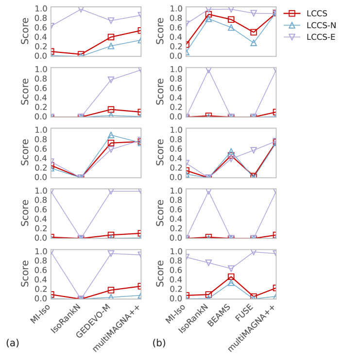
Figure A7: LCCS for the five network sets (Yeast+%LC, PHY1, PHY2, Y2H1, and Y2H2 from top to bottom) for (a) topology-only alignments and (b) topology+sequence alignments.

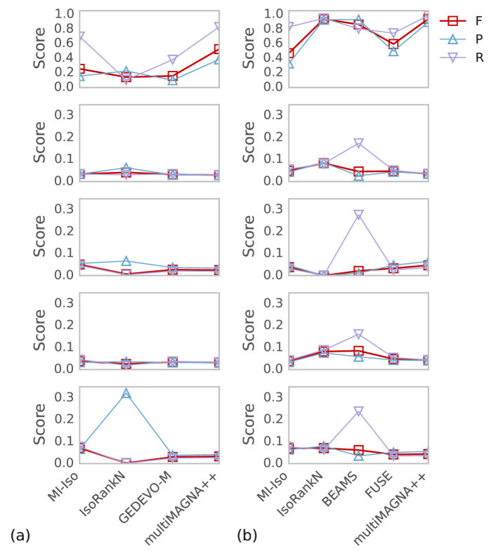
Figure A8: F-score for the five network sets (Yeast+%LC, PHY1, PHY2, Y2H1, and Y2H2 from top to bottom) for (a) topology-only alignments and (b) topology+sequence alignments.

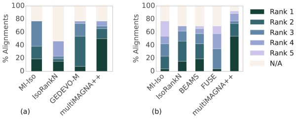
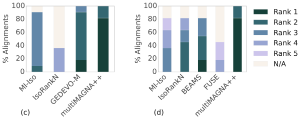
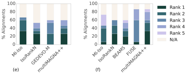
Figure A9: Ranking of the MNA methods across all of Yeast+%LC, PHY1, PHY2, Y2H1, and Y2H2 network sets with respect to (a-b) all measures, (c-d) topological NCV-MNC, NCV-CIQ, and LCCS measures, and (e-f) functional MNE, GC, and F-score measures, for (a,c,e) topology-only alignments and (b,d,f) topology+sequence alignments. The ranking of each method is expressed as a percentage of all evaluation tests in which the given method is the best performing (“Rank 1”), the second best performing (“Rank 2”), etc. aligner of all considered methods. By “best”, we mean the method with the lowest $p$-value, or the method with the best alignment quality score if the $p$-values are tied. If an alignment score of a method is not statistically significant, the method is not ranked and is labelled as “N/A”.

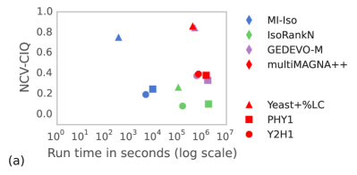
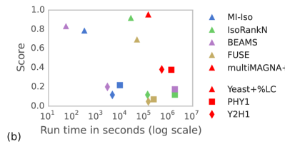
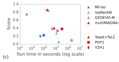
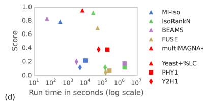
Figure A13: NCV-CIQ as a function of time when using (a-b) a single thread and (c-d) 64 threads, for (a,c) topology-only alignments and (b,d) topology+sequence alignments, for the three network sets with more than two networks (we leave out these results for PHY2 and Y2H2 that have two networks each; Section 2.2.1). For equivalent results for the remaining measures, see Figures S8 and S9.

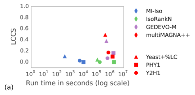
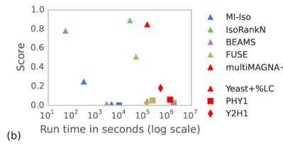
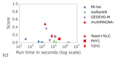
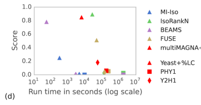
Figure A14: LCCS as a function of time when using (a-b) a single thread and (c-d) 64 threads, for (a,c) topology-only alignments and (b,d) topology+sequence alignments, for the three network sets with more than two networks (we leave out these results for PHY2 and Y2H2 that have two networks each).

SUPPLEMENTARY TABLES

Set	Species	Proteins	Interactions
Yeast+%LC	Yeast+0%LC	1,004	8,323
	Yeast+5%LC	1,004	8,739
	Yeast+10%LC	1,004	9,155
	Yeast+15%LC	1,004	9,571
	Yeast+20%LC	1,004	9,987
	Yeast+25%LC	1,004	10,403
PHY1	Fly	7,887	36,285
	Worm	3,006	5,506
	Yeast	6,168	82,368
	Human	16,061	157,650
PHY2	Yeast	768	13,654
	Human	8,283	19,697
Y2H1	Fly	7,097	23,370
	Worm	2,874	5,199
	Yeast	3,427	11,348
	Human	9,996	39,984
Y2H2	Yeast	744	966
	Human	1,191	1,567

Table A3: The five PPI networks sets that we use in our study. We know the true mapping for the Yeast+%LC network set unlike for the other network sets. For PHY2 and Y2H2, we only use the yeast and human PPI networks since the fly and worm networks are too small for analysis.

Algorithms	Parameters
Topology-only alignments
IsoRankN	K=30 thresh=1e-4 maxveclen=5000000 alpha=1.0
MI-Iso	K=30 thresh=1e-4 maxveclen=5000000 alpha=1.0
GEDEVO-M	beta=0.4
multiMAGNA++	m=CIQ p=15000 n=100000 e=0.5 a=1.0
Topology+sequence alignments
IsoRankN	K=30 thresh=1e-4 maxveclen=5000000 alpha=0.5
MI-Iso	K=30 thresh=1e-4 maxveclen=5000000 alpha=1.0
BEAMS	beta=0.4 alpha=0.5
FUSE	k=[100,100,100,100] iter_num=1000 gamma=0.7 a=0.5
multiMAGNA++	m=CIQ p=15000 n=100000 e=0.5 a=0.25

Table A4: Parameters of the MNA methods. For the existing methods, we use parameters that were recommended in the methods’ original publications. The parameters of multiMAGNA++ are the edge conservation measure (m), population size (p), number of generations (n), and the $\alpha$ parameter (a).

	Topological measures			Functional measures
Method	NCV-MNC	NCV-CIQ	LCCS	MNE	GC	F-score
MI-Iso	0.3533 p $<$ 1.00e-4	0.7526 p $<$ 1.00e-4	0.1042 p $<$ 1.00e-4	0.9578 p $<$ 1.00e-4	0.5143 p $<$ 1.00e-4	0.2558 p $<$ 1.00e-4
IsoRankN	0.0730 p $<$ 1.00e-4	0.2655 p $<$ 1.00e-4	0.0446 p = 0.026	0.9630 p $<$ 1.00e-4	0.7376 p $<$ 1.00e-4	0.1420 p $<$ 1.00e-4
GEDEVO-M	0.2969 p $<$ 1.00e-4	0.8574 p $<$ 1.00e-4	0.4104 p $<$ 1.00e-4	0.9610 p $<$ 1.00e-4	0.4333 p $<$ 1.00e-4	0.1586 p $<$ 1.00e-4
multiMAGNA++	0.5578 p $<$ 1.00e-4	0.8991 p $<$ 1.00e-4	0.5501 p $<$ 1.00e-4	0.9341 p $<$ 1.00e-4	0.7739 p $<$ 1.00e-4	0.5258 p $<$ 1.00e-4

Table A5: Alignment accuracy of different MNA approaches for the Yeast+%LC network set in terms of topological NCV-MNC, NCV-CIQ, and LCCS measures and functional MNE, GO correctness (GC), and F-score measures, for topology-only alignments. The symbol “p” signifies $p$-values of the observed alignment scores, as defined in Section 2.2.2. For each alignment quality measure (i.e., in each column), the best method (i.e., the method with the lowest $p$-value, or the method with the best alignment quality score if the $p$-values are tied) is bolded. The alignment scores that are not statistically significant, if any, are greyed out and italicized. Note that for MNE, the lower the score, the better the alignment quality. For all other measures, the higher the score, the better the alignment quality.

	Topological measures			Functional measures
Method	NCV-MNC	NCV-CIQ	LCCS	MNE	GC	F-score
MI-Iso	0.5638 p $<$ 1.00e-4	0.7908 p $<$ 1.00e-4	0.2508 p $<$ 1.00e-4	0.9508 p $<$ 1.00e-4	0.6137 p $<$ 1.00e-4	0.4709 p $<$ 1.00e-4
IsoRankN	0.8967 p $<$ 1.00e-4	0.9219 p $<$ 1.00e-4	0.8929 p $<$ 1.00e-4	0.9532 p $<$ 1.00e-4	0.9748 p $<$ 1.00e-4	0.9367 p $<$ 1.00e-4
BEAMS	0.8215 p $<$ 1.00e-4	0.8342 p $<$ 1.00e-4	0.7827 p $<$ 1.00e-4	0.9667 p $<$ 1.00e-4	0.9882 p $<$ 1.00e-4	0.8625 p $<$ 1.00e-4
FUSE	0.6299 p $<$ 1.00e-4	0.6943 p $<$ 1.00e-4	0.5123 p $<$ 1.00e-4	0.9618 p $<$ 1.00e-4	0.7744 p $<$ 1.00e-4	0.5953 p $<$ 1.00e-4
multiMAGNA++	0.9241 p $<$ 1.00e-4	0.9574 p $<$ 1.00e-4	0.9201 p $<$ 1.00e-4	0.9347 p $<$ 1.00e-4	0.9897 p $<$ 1.00e-4	0.9392 p $<$ 1.00e-4

Table A6: Alignment accuracy of different MNA approaches for the Yeast+%LC network set in terms of topological NCV-MNC, NCV-CIQ, and LCCS measures and functional MNE, GO correctness (GC), and F-score measures, for topology+sequence alignments. The symbol “p” signifies $p$-values of the observed alignment scores. For each alignment quality measure (i.e., in each column), the best method (i.e., the method with the lowest $p$-value, or the method with the best alignment quality score if the $p$-values are tied) is bolded. The alignment scores that are not statistically significant, if any, are greyed out and italicized. Note that for MNE, the lower the score, the better the alignment quality. For all other measures, the higher the score, the better the alignment quality.

		Topological measures		Functional measures
	Method	NCV-CIQ	LCCS	MNE	GC	F-score
PHY2	MI-Iso	0.2746 p $<$ 1.00e-4	0.2632 p $<$ 1.00e-4	0.9736 p = 3.00e-4	0.4034 p $<$ 1.00e-4	0.0503 p $<$ 1.00e-4
	IsoRankN	0.0000 p = 1.000	0.0000 p = 1.000	1.0000 p = 0.376	0.2521 p = 0.009	0.0067 p = 0.382
	BEAMS	0.5858 p $<$ 1.00e-4	0.4714 p $<$ 1.00e-4	0.9799 p $<$ 1.00e-4	0.5833 p = 1.000	0.0210 p $<$ 1.00e-4
	FUSE	0.0561 p = 0.002	0.0352 p = 0.249	0.9808 p = 0.271	0.2422 p $<$ 1.00e-4	0.0332 p $<$ 1.00e-4
	GEDEVO-M	0.5562 p $<$ 1.00e-4	0.7369 p $<$ 1.00e-4	0.9786 p = 0.042	0.2096 p $<$ 1.00e-4	0.0266 p $<$ 1.00e-4
	multiMAGNA++	0.5236 p $<$ 1.00e-4	0.7680 p $<$ 1.00e-4	0.9745 p = 1.00e-4	0.3033 p $<$ 1.00e-4	0.0466 p $<$ 1.00e-4
Y2H2	MI-Iso	0.2972 p $<$ 1.00e-4	0.0970 p $<$ 1.00e-4	0.9880 p = 0.313	0.5567 p = 0.131	0.0710 p $<$ 1.00e-4
	IsoRankN	0.2853 p $<$ 1.00e-4	0.0965 p $<$ 1.00e-4	0.9885 p = 0.641	0.3651 p $<$ 1.00e-4	0.0706 p $<$ 1.00e-4
	BEAMS	0.6020 p $<$ 1.00e-4	0.4741 p $<$ 1.00e-4	0.9869 p = 0.057	0.8222 p = 0.783	0.0616 p $<$ 1.00e-4
	FUSE	0.0707 p = 0.028	0.0518 p = 0.889	0.9949 p = 0.644	0.2801 p $<$ 1.00e-4	0.0416 p $<$ 1.00e-4
	GEDEVO-M	0.6945 p $<$ 1.00e-4	0.1905 p $<$ 1.00e-4	0.9968 p = 0.926	0.2228 p = 0.714	0.0303 p = 0.486
	multiMAGNA++	0.7307 p $<$ 1.00e-4	0.2727 p $<$ 1.00e-4	0.9908 p = 0.090	0.2920 p $<$ 1.00e-4	0.0436 p $<$ 1.00e-4

Table A7: Alignment accuracy selected of different MNA approaches for the PHY2 and Y2H2 network sets in terms of topological NCV-CIQ and LCCS measures and functional MNE, GO correctness (GC), and F-score measures. The symbol “p” signifies $p$-values of the observed alignment scores. For each alignment quality measure, and for each network set, the best method (i.e., the method with the lowest $p$-value, or the method with the best alignment quality score if the $p$-values are tied) is bolded. The alignment scores that are not statistically significant, if any, are greyed out and italicized. Note that for MNE, the lower the score, the better the alignment quality. For all other measures, the higher the score, the better the alignment quality.

		Topological measures		Functional measures
	Method	NCV-CIQ	LCCS	MNE	GC	F-score
PHY1	MI-Iso	0.2472 p $<$ 1.00e-4	0.0000 p = 1.000	0.8912 p = 0.579	0.1913 p $<$ 1.00e-4	0.0341 p $<$ 1.00e-4
	IsoRankN	0.1012 p $<$ 1.00e-4	0.0000 p = 1.000	0.7977 p $<$ 1.00e-4	0.2535 p $<$ 1.00e-4	0.0415 p $<$ 1.00e-4
	GEDEVO-M	0.3554 p $<$ 1.00e-4	0.1613 p $<$ 1.00e-4	0.9205 p = 1.000	0.1721 p $<$ 1.00e-4	0.0324 p $<$ 1.00e-4
	multiMAGNA++	0.4046 p $<$ 1.00e-4	0.1064 p $<$ 1.00e-4	0.8449 p $<$ 1.00e-4	0.1610 p $<$ 1.00e-4	0.0299 p $<$ 1.00e-4
PHY2	MI-Iso	0.2746 p $<$ 1.00e-4	0.2632 p $<$ 1.00e-4	0.9889 p = 0.858	0.4034 p $<$ 1.00e-4	0.0503 p $<$ 1.00e-4
	IsoRankN	0.0000 p = 1.000	0.0000 p = 1.000	0.9863 p = 0.382	0.2521 p = 0.009	0.0067 p = 0.382
	GEDEVO-M	0.5562 p $<$ 1.00e-4	0.7369 p $<$ 1.00e-4	0.9786 p = 0.042	0.2096 p $<$ 1.00e-4	0.0266 p $<$ 1.00e-4
	multiMAGNA++	0.5236 p $<$ 1.00e-4	0.7680 p $<$ 1.00e-4	0.9745 p = 1.00e-4	0.1952 p = 0.001	0.0249 p = 1.00e-4
Y2H1	MI-Iso	0.1935 p $<$ 1.00e-4	0.0264 p $<$ 1.00e-4	0.9229 p = 0.995	0.2092 p $<$ 1.00e-4	0.0382 p $<$ 1.00e-4
	IsoRankN	0.0815 p $<$ 1.00e-4	0.0000 p = 1.000	0.8447 p $<$ 1.00e-4	0.1736 p = 0.304	0.0255 p $<$ 1.00e-4
	GEDEVO-M	0.4511 p $<$ 1.00e-4	0.0722 p $<$ 1.00e-4	0.9032 p = 0.919	0.1879 p = 6.00e-4	0.0347 p $<$ 1.00e-4
	multiMAGNA++	0.4943 p $<$ 1.00e-4	0.1088 p $<$ 1.00e-4	0.8899 p = 6.00e-4	0.1794 p = 0.124	0.0322 p = 0.719
Y2H2	MI-Iso	0.2972 p $<$ 1.00e-4	0.0970 p $<$ 1.00e-4	0.9880 p = 0.313	0.5567 p = 0.131	0.0710 p $<$ 1.00e-4
	IsoRankN	0.0000 p = 1.000	0.0000 p = 1.000	0.9885 p = 0.641	0.3333 p = 0.870	0.0022 p = 0.214
	GEDEVO-M	0.6945 p $<$ 1.00e-4	0.1905 p $<$ 1.00e-4	0.9968 p = 0.926	0.2228 p = 0.714	0.0303 p = 0.486
	multiMAGNA++	0.7307 p $<$ 1.00e-4	0.2727 p $<$ 1.00e-4	0.9926 p = 0.271	0.2342 p = 0.354	0.0328 p = 0.069

Table A8: Alignment accuracy of different MNA approaches for the PHY1, PHY2, Y2H1 and Y2H2 network sets in terms of topological NCV-CIQ and LCCS measures and functional MNE, GO correctness (GC), and F-score measures, for topology-only alignments. The symbol “p” signifies $p$-values of the observed alignment scores. For each alignment quality measure, and for each network set, the best method (i.e., the method with the lowest $p$-value, or the method with the best alignment quality score if the $p$-values are tied) is bolded. The alignment scores that are not statistically significant, if any, are greyed out and italicized. Note that for MNE, the lower the score, the better the alignment quality. For all other measures, the higher the score, the better the alignment quality.

		Topological measures		Functional measures
	Method	NCV-CIQ	LCCS	MNE	GC	F-score
PHY1	MI-Iso	0.2517 p $<$ 1.00e-4	0.0000 p = 1.000	0.8224 p $<$ 1.00e-4	0.2732 p $<$ 1.00e-4	0.0492 p $<$ 1.00e-4
	IsoRankN	0.1336 p = 1.00e-4	0.0258 p $<$ 1.00e-4	0.8773 p = 1.000	0.3279 p $<$ 1.00e-4	0.0838 p $<$ 1.00e-4
	BEAMS	0.3250 p $<$ 1.00e-4	0.0000 p = 1.000	0.8944 p = 0.895	0.4084 p = 1.000	0.0457 p $<$ 1.00e-4
	FUSE	0.0679 p = 5.00e-4	0.0000 p = 1.000	0.8781 p $<$ 1.00e-4	0.2268 p $<$ 1.00e-4	0.0472 p $<$ 1.00e-4
	multiMAGNA++	0.3884 p $<$ 1.00e-4	0.1064 p $<$ 1.00e-4	0.8622 p $<$ 1.00e-4	0.1759 p $<$ 1.00e-4	0.0353 p $<$ 1.00e-4
PHY2	MI-Iso	0.1670 p $<$ 1.00e-4	0.1537 p = 4.00e-4	0.9736 p = 3.00e-4	0.2807 p $<$ 1.00e-4	0.0381 p $<$ 1.00e-4
	IsoRankN	0.0000 p = 1.000	0.0000 p = 1.000	1.0000 p = 0.376	0.0000 p = 1.000	0.0000 p = 1.000
	BEAMS	0.5858 p $<$ 1.00e-4	0.4714 p $<$ 1.00e-4	0.9799 p $<$ 1.00e-4	0.5833 p = 1.000	0.0210 p $<$ 1.00e-4
	FUSE	0.0561 p = 0.002	0.0352 p = 0.249	0.9808 p = 0.271	0.2422 p $<$ 1.00e-4	0.0332 p $<$ 1.00e-4
	multiMAGNA++	0.5226 p $<$ 1.00e-4	0.7578 p $<$ 1.00e-4	0.9748 p = 2.00e-4	0.3033 p $<$ 1.00e-4	0.0466 p $<$ 1.00e-4
Y2H1	MI-Iso	0.1354 p $<$ 1.00e-4	0.0000 p = 1.000	0.8992 p = 0.396	0.1990 p $<$ 1.00e-4	0.0379 p $<$ 1.00e-4
	IsoRankN	0.1315 p $<$ 1.00e-4	0.0264 p $<$ 1.00e-4	0.9003 p = 0.031	0.3247 p $<$ 1.00e-4	0.0822 p $<$ 1.00e-4
	BEAMS	0.2856 p $<$ 1.00e-4	0.0000 p = 1.000	0.9159 p = 0.363	0.3945 p $<$ 1.00e-4	0.0856 p $<$ 1.00e-4
	FUSE	0.0480 p $<$ 1.00e-4	0.0000 p = 1.000	0.8781 p $<$ 1.00e-4	0.2369 p $<$ 1.00e-4	0.0483 p $<$ 1.00e-4
	multiMAGNA++	0.4383 p $<$ 1.00e-4	0.0722 p $<$ 1.00e-4	0.8954 p = 0.062	0.2040 p $<$ 1.00e-4	0.0428 p $<$ 1.00e-4
Y2H2	MI-Iso	0.2035 p $<$ 1.00e-4	0.0773 p = 2.00e-4	0.9913 p = 0.604	0.4554 p = 0.783	0.0693 p = 0.082
	IsoRankN	0.2853 p $<$ 1.00e-4	0.0965 p $<$ 1.00e-4	0.9945 p = 0.704	0.3651 p $<$ 1.00e-4	0.0706 p $<$ 1.00e-4
	BEAMS	0.6020 p $<$ 1.00e-4	0.4741 p $<$ 1.00e-4	0.9869 p = 0.057	0.8222 p = 0.783	0.0616 p $<$ 1.00e-4
	FUSE	0.0707 p = 0.028	0.0518 p = 0.889	0.9949 p = 0.644	0.2801 p $<$ 1.00e-4	0.0416 p $<$ 1.00e-4
	multiMAGNA++	0.7125 p $<$ 1.00e-4	0.2361 p $<$ 1.00e-4	0.9908 p = 0.090	0.2920 p $<$ 1.00e-4	0.0436 p $<$ 1.00e-4

Table A9: Alignment accuracy of different MNA approaches for the PHY1, PHY2, Y2H1 and Y2H2 network sets in terms of topological NCV-CIQ and LCCS measures and functional MNE, GO correctness (GC), and F-score measures, for topology+sequence alignments. The symbol “p” signifies $p$-values of the observed alignment scores. For each alignment quality measure, and for each network set, the best method (i.e., the method with the lowest $p$-value, or the method with the best alignment quality score if the $p$-values are tied) is bolded. The alignment scores that are not statistically significant, if any, are greyed out and italicized. Note that for MNE, the lower the score, the better the alignment quality. For all other measures, the higher the score, the better the alignment quality.

References

- Alkan and Erten (2014) Alkan, F. and Erten, C. (2014). BEAMS: backbone extraction and merge strategy for the global many-to-many alignment of multiple PPI networks. Bioinformatics, 30(4), 531–539.
- Bäck (1996) Bäck, T. (1996). Evolutionary algorithms in theory and practice evolution strategies, evolutionary programming, genetic algorithms. Oxford University Press, New York.
- Bayati et al. (2009) Bayati, M., Gerritsen, M., Gleich, D., Saberi, A., and Wang, Y. (2009). Algorithms for large, sparse network alignment problems. In Data Mining, 2009. ICDM ’09. Ninth IEEE International Conference on, pages 705–710.
- Breitkreutz et al. (2008) Breitkreutz, B. J., Stark, C., T., R., L., B., Breitkreutz, A., Livstone, M., Oughtred, R., Lackner, D., Bähler, J., Wood, V., Dolinski, K., and Tyers, M. (2008). The BioGRID Interaction Database: 2008 update. Nucleic Acids Research, 36(Database issue), D637–D640.
- Clark and Kalita (2014) Clark, C. and Kalita, J. (2014). A comparison of algorithms for the pairwise alignment of biological networks. Bioinformatics, 30(16), 2351–2359.
- Clark and Kalita (2015) Clark, C. and Kalita, J. (2015). A multiobjective memetic algorithm for PPI network alignment. Bioinformatics, 31(12), 1988–1998.
- Collins et al. (2007) Collins, S., Kemmeren, P., Zhao, X., Greenblatt, J., Spencer, F., Holstege, F., Weissman, J., and Krogan, N. (2007). Toward a comprehensive atlas of the physical interactome of saccharomyces cerevisiae. Molecular Cell Proteomics, 6(3), 439–450.
- Conte et al. (2004) Conte, D., Foggia, P., Sansone, C., and Vento, M. (2004). Thirty years of graph matching in pattern recognition. International Journal of Pattern Recognition and Artificial Intelligence, 18(03), 265–298.
- Crawford and Milenković (2015) Crawford, J. and Milenković, T. (2015). GREAT: GRaphlet Edge-based network AlignmenT. In Proc. of the IEEE Int. Conf. on Bioinformatics and Biomedicine (BIBM).
- Crawford et al. (2015) Crawford, J., Sun, Y., and Milenković, T. (2015). Fair evaluation of global network aligners. Algorithms for Molecular Biology, 10(19).
- Cusick et al. (2009) Cusick, M. E., Yu, H., Smolyar, A., and Vidal, M. (2009). Literature-curated protein interaction datasets. Nature Methods, 6, 39–46.
- Duchenne et al. (2011) Duchenne, O., Bach, F., Kweon, I.-S., and Ponce, J. (2011). A tensor-based algorithm for high-order graph matching. Pattern Analysis and Machine Intelligence, IEEE Transactions on, 33(12), 2383–2395.
- Elmsallati et al. (2015) Elmsallati, A., Clark, C., and Kalita, J. (2015). Global alignment of protein-protein interaction networks: A survey. IEEE/ACM Trans. on Computational Biology and Bioinformatics, 2015(Epub ahead of print).
- Faisal et al. (2014) Faisal, F., Zhao, H., and Milenković, T. (2014). Global network alignment in the context of aging. IEEE/ACM Transactions on Computational Biology and Bioinformatics, 12(1), 40–52.
- Faisal et al. (2015) Faisal, F., Meng, L., Crawford, J., and Milenković, T. (2015). The post-genomic era of biological network alignment. EURASIP Journal on Bioinformatics and Systems Biology, 2015(1).
- Gligorijević et al. (2015) Gligorijević, V., Malod-Dognin, N., and Pržulj, N. (2015). FUSE: Multiple Network Alignment via Data Fusion. Bioinformatics, 2015(Epub ahead of print).
- Hu et al. (2014) Hu, J., Kehr, B., and Reinert, K. (2014). NetCoffee: a fast and accurate global alignment approach to identify functionally conserved proteins in multiple networks. Bioinformatics, 30(4), 540–548.
- Ibragimov et al. (2013a) Ibragimov, R., Malek, M., and Baumbach, J. (2013a). GEDEVO: An evolutionary graph edit distance algorithm for biological network alignment. In GCB, pages 68–79.
- Ibragimov et al. (2013b) Ibragimov, R., Malek, M., Guo, J., and Baumbach, J. (2013b). NABEECO: Biological Network Alignment with Bee Colony Optimization Algorithm. In Proc. of Annual Conf. on Genetic and Evolutionary Computation, pages 43–44.
- Ibragimov et al. (2014) Ibragimov, R., Malek, M., Guo, J., and Baumbach, J. (2014). Multiple graph edit distance - simultaneous topological alignment of multiple protein-protein interaction networks with an evolutionary algorithm. In Proc. of Annual Conf. on Genetic and Evolutionary Computation, pages 277–284.
- Jeong and Yoon (2015) Jeong, H. and Yoon, B.-J. (2015). Accurate multiple network alignment through context-sensitive random walk. BMC Systems Biology, 9(Suppl. 1), S7.
- Jeong et al. (2000) Jeong, H., Tombor, B., Albert, R., Oltvai, Z. N., and Barabási, A.-L. (2000). The large-scale organization of metabolic networks. Nature, 407, 651–654.
- Kollias et al. (2012) Kollias, G., Mohammadi, S., and Grama, A. (2012). Network Similarity Decomposition (NSD): A fast and scalable approach to network alignment. Knowledge and Data Engineering, IEEE Transactions on, 24(12), 2232–2243.
- Koutra et al. (2013) Koutra, D., Tong, H., and Lubensky, D. (2013). BIG-ALIGN: fast bipartite graph alignment. In 2013 IEEE 13th International Conference on Data Mining, Dallas, TX, USA, December 7-10, 2013, pages 389–398.
- Kuchaiev and Pržulj (2011) Kuchaiev, O. and Pržulj, N. (2011). Integrative network alignment reveals large regions of global network similarity in yeast and human. Bioinformatics, 27(10), 1390–1396.
- Kuchaiev et al. (2010) Kuchaiev, O., Milenković, T., Memišević, V., Hayes, W., and Pržulj, N. (2010). Topological network alignment uncovers biological function and phylogeny. Journal of The Royal Society Interface, 7(50), 1341–1354.
- Liao et al. (2009) Liao, C., Lu, K., Baym, M., Singh, R., and Berger, B. (2009). IsoRankN: Spectral methods for global alignment of multiple protein networks. Bioinformatics, 25(12), i253–258.
- Memis̆ević and Prz̆ulj (2012) Memis̆ević, V. and Prz̆ulj, N. (2012). C-GRAAL: common-neighbors-based global GRAph ALignment of biological networks. Integrative Biology, 4(7), 734–743.
- Meng et al. (2015) Meng, L., Striegel, A., and Milenković, T. (2015). Local versus global biological network alignment. arXiv:1509.08524 [q-bio.MN].
- Milenković and Pržulj (2008) Milenković, T. and Pržulj, N. (2008). Uncovering biological network function via graphlet degree signatures. Cancer Informatics, 6, 257–273.
- Milenković et al. (2010) Milenković, T., Ng, W., Hayes, W., and Pržulj, N. (2010). Optimal network alignment with graphlet degree vectors. Cancer Informatics, 9, 121–137.
- Mulder et al. (2014) Mulder, N. J., Akinola, R. O., Mazandu, G. K., and Rapanoel, H. (2014). Using biological networks to improve our understanding of infectious diseases. Comput. Struct. Biotechnol. J., 11(18), 1–10.
- Neyshabur et al. (2013) Neyshabur, B., Khadem, A., Hashemifar, S., and Shahriar Arab, S. (2013). NETAL: a new graph-based method for global alignment of protein-protein interaction networks. Bioinformatics, 29(13), 1654–1662.
- Patro and Kingsford (2012) Patro, R. and Kingsford, C. (2012). Global network alignment using multiscale spectral signatures. Bioinformatics, 28(23), 3105–3114.
- Sahraeian and Yoon (2013) Sahraeian, S. M. E. and Yoon, B.-J. (2013). SMETANA: Accurate and scalable algorithm for probabilistic alignment of large-scale biological networks. PLOS ONE, 8(7), 679395.
- Saraph and Milenković (2014) Saraph, V. and Milenković, T. (2014). MAGNA: Maximizing accuracy in global network alignment. Bioinformatics, 30(20), 2931–2940.
- Sharan and Ideker (2006a) Sharan, R. and Ideker, T. (2006a). Modeling cellular machinery through biological network comparison. Nat. Biotechnol., 24(4), 427–433.
- Sharan and Ideker (2006b) Sharan, R. and Ideker, T. (2006b). Modeling cellular machinery through biological network comparison. Nature Biotechnology, 24, 427–433.
- Sharan et al. (2007) Sharan, R., Ulitsky, I., and Shamir, R. (2007). Network-based prediction of protein function. Mol. Reprod. Dev., 3(88), 1–13.
- Singh et al. (2007) Singh, R., Xu, J., and Berger, B. (2007). Pairwise global alignment of protein interaction networks by matching neighborhood topology. In Research in computational molecular biology, pages 16–31. Springer.
- Stuart et al. (2003) Stuart, J. M., Segal, E., Koller, D., and Kim, S. K. (2003). A gene-coexpression network for global discovery of conserved genetic modules. Science, 302(5643), 249–255.
- Sun et al. (2015) Sun, Y., Crawford, J., Tang, J., and Milenković, T. (2015). Simultaneous optimization of both node and edge conservation in network alignment via WAVE. In Proc. of Workshop on Algorithms in Bioinformatics (WABI), pages 16–39.
- The Gene Ontology Consortium (2000) The Gene Ontology Consortium (2000). Gene ontology: tool for the unification of biology. Nature Genetics, 25, 25–29.
- Torresani et al. (2008) Torresani, L., Kolmogorov, V., and Rother, C. (2008). Feature correspondence via graph matching: Models and global optimization. In Proc. of ECCV, volume 5303 of Lecture Notes in Computer Science, pages 596–609. Springer Berlin Heidelberg.
- Vijayan et al. (2015) Vijayan, V., Saraph, V., and Milenković, T. (2015). MAGNA++: Maximizing Accuracy in Global Network Alignment via both node and edge conservation. Bioinformatics, 31(14), 2409–2411.
- Wang et al. (2011) Wang, H., Huang, H., and Ding, C. (2011). Simultaneous clustering of multi-type relational data via symmetric nonnegative matrix tri-factorization. In Proc. of ACM Int. Conf. on Information and Knowledge Management.
- Ye et al. (2006) Ye, J., McGinnis, S., and Madden, T. L. (2006). BLAST: improvements for better sequence analysis. Nucleic Acids Research, 34(Web Server issue), W6–W9.