Harmonic expansion of the effective potential in Functional Renormalization Group at finite chemical potential

Abstract

In this paper we propose a method to study the Functional Renormalization Group at finite chemical potential. The method consists of mapping the FRG equations within the Fermi surface into a differential equation defined on a rectangle with zero boundary conditions. To solve this equation we use an expansion of the potential in a harmonic basis. With this method we determined the phase diagram of a simple Yukawa-type model; as expected, the bosonic fluctuations decrease the strength of the transition.

I Introduction

The Functional Renormalization Group (FRG) Gies:2006wv is a powerful nonperturbative method, it is nowadays a fair alternative to other exact numerical methods, like the Monte Carlo lattice simulations. Besides zero temperature applications Gies:2006wv there are efforts to adapt it to finite temperature and chemical potential case Herbst:2013ail ; Drews:2013hha ; Drews:2014wba ; Drews:2014spa ; Posfay:2015fpa ; Eser:2015pka . A particularly interesting challenge is to reveal the equations of state of the strong interaction, as this information could be directly used in heavy ion collisions Herbst:2013ail and in physics of compact astrophysical objects Drews:2014spa .

There are different formulation for the exact functional equation that forms the basis of FRG computations, in this paper we will use Wetterich equation Wetterich:1989xg ; Wetterich:1992yh . One can also use different regulators Nandori:2012tc , here we use Litim’s regulator Litim:2001up . The Wetterich equation is exact, but is valid in infinite dimensional operator space. In practice one has to restrict the operator content to a finite set, ie. we have to use an Ansatz for the effective action, and follow the scale dependence only of terms present in this Ansatz. A popular choice for bosonic systems is the Local Polynomial Approximation (LPA), eventually extending it to wave function renormalization effects (LPA’), for fermions restricting only to the renormalizable operators (for fermions there exists also variants of the LPA method Jakovac:2014lqa ).

The LPA (LPA’) still provides a nonlinear partial differential equation for the effective potential. For an analytic treatment, one can power expand the effective potential, then we obtain a series of ordinary differential equations for the scale dependence of the coupling constants. With increasing number of terms taken into account, one may hope that the solution converges to the exact solution; as in some cases it can be really demonstrated Mati:2014xma .

Alternatively, one can discretize the potential, representing the function with values taken at discrete points. This again leads to a series of ordinary differential equations, and in principle with raising the density of the representing points it will reproduce the complete smooth function. Although this method seems to be very promising, in practice it turns to be badly conditioned, very sensitive to numerical errors Posfay:2015fpa . There are therefore variants of these methods to provide better convergence Adams:1995cv ; Fukushima:2010ji .

At finite temperature and chemical potential the Bose-Einstein or Fermi-Dirac distributions also appear in the FRG equations, which makes the effective treatment of the LPA equations even more tedious. Particularly at small temperatures and finite chemical potential the Fermi-Dirac distribution becomes a near step function, this makes the polynomial expansion useless, and the convergence properties of the discretized version even worse.

Another unpleasant property of the discretized numerical method is that the resulting infrared (IR) effective potential at zero scale $k=0$ is strictly convex. At one hand it is a well known behavior of the exact result obtained through Legendre transformation Litim:2006nn , but for field theoretical application the coarse grained effective potential is much more comfortable to use, in particular to identify a phase transition. The polynomial expansion method, similarly to the conventional perturbation theory naturally provides this potential, while in the discretized version the coarse grained potential can be defined only at finite scale.

All this suggests that an analytic method similar to the polynomial expansion working also at finite temperature and chemical potential could be very useful. In this paper we propose such a method, first studying the extreme case having zero temperature and finite fermionic chemical potential. To demonstrate the way it is working we will use a simple model with one bosonic and one fermionic degree of freedom, coupled with Yukawa interaction. In order to find the scale dependent effective potential $U(k,\varphi)$, we can realize that the Fermi surface splits the $k-\varphi$ space into two parts, where the corresponding FRG equations are different. One should solve the FRG equations at each domain, and require that the solution is continuous at the border line. The strategy we follow is to map the above problem to another one where the Fermi surface is a rectangle, and we have zero boundary conditions. Then we can use some function basis, in the present case a harmonic basis, and solve the ordinary differential equation arising for the coefficients. There are other possible choices for the function base, recently in papers Borchardt:2015rxa ; Borchardt:2016xju ; Borchardt:2016pif the authors used Chebyshev polynomials.

We will discuss the convergence properties of our method, and find out, how a coarse grained effective potential can be read off. With this information we are able to identify the phase transition point as well as explore the position of the borderline of the first and second order phase transitions in the coupling constant space.

The structure of the paper is the following. After the Introduction, in Section II, we introduce our model, write up the FRG Ansatz, determine the FRG equations at finite temperature and chemical potential, and at zero temperature we identify the Fermi-surface. In Section III we discuss the coordinate transformation needed to map the Fermi surface to a rectangle, leaving the symmetries of the system intact. In Section IV we propose a basis to handle the partial differential equation at hand, and discuss the solution strategy. In Section V we discuss the results: the effective potential at different approximation level, the appearance of the first and second order phase transition, and finally the order of the phase transition as a function of the couplings, comparing it to the mean field analysis. The paper is closed with a Conclusion section VI.

II The model and the FRG equation

We will use a simple Yukawa-type model with one bosonic and one fermionic degree of freedom described by the bare action (defined at scale $\Lambda$)

$$\Gamma_{\Lambda}[\varphi,\psi]=\int d^{4}x\left[\bar{\psi}(i\mbox{\hskip 2.65451pt/$\partial$}-g_{0}\varphi)\psi+\frac{1}{2}(\partial_{\mu}\varphi)^{2}-\frac{m_{0}^{2}}{2}\varphi^{2}-\frac{\lambda_{0}}{24}\varphi^{4}\right].$$ (1)

This model has two phases, in the symmetric phase the fermion is massless, in the spontaneously broken (SSB) phase the fermion mass is $g\left\langle{\varphi}\right\rangle$.

As we want to treat this model with FRG, we need an Ansatz for the effective action at scale $k$. Since in this paper the main goal is to demonstrate the way how the finite chemical potential can be treated, we choose the simplest possible Ansatz, where only the bosonic effective potential depends on the scale:

$$\Gamma_{k}[\varphi,\psi]=\int d^{4}x\left[\bar{\psi}(i\mbox{\hskip 2.65451pt/$\partial$}-g\varphi)\psi+\frac{1}{2}(\partial_{\mu}\varphi)^{2}-U_{k}(\varphi)\right].$$ (2)

Although here neither wave function renormalization, nor the running of the Higgs coupling are taken into account, both effects can be easily adapted into the present method.

The Wetterich equation for this model reads

$$\partial_{k}U_{k}=\frac{1}{2}\mathop{\mathrm{STr}}\ln(R_{k}+\Gamma_{k}^{(2)}),$$ (3)

where STr means super-trace, $R_{k}$ is the regulator functional, and $\Gamma_{k}^{(2)}$ is the second functional derivative of the effective action. Using three-dimensional Litim’s regulator, the corresponding Wetterich equation reads at finite temperature $T$ and at finite chemical potential $\mu$

$$\partial_{k}U_{k}=\frac{k^{4}}{12\pi^{2}}\left[\frac{1+2n_{B}(\omega_{B})}{\omega_{B}}+4\frac{-1+n_{F}(\omega_{F}-\mu)+n_{F}(\omega_{F}+\mu)}{\omega_{F}}\right],$$ (4)

where $n_{B}$ and $n_{F}$ are the Bose-Einstein and the Fermi-Dirac distributions, respectively

$$n_{B/F}(\omega)=\frac{1}{1\mp e^{-\beta\omega}},$$ (5)

where $\beta=1/T$, while

$$\omega_{B}^{2}=k^{2}+\partial_{\varphi}^{2}U,\qquad\omega_{F}^{2}=k^{2}+g^{2}\varphi^{2}.$$ (6)

The initial condition of this equation is

$$U_{\Lambda}(\varphi)=\frac{m_{0}^{2}}{2}\varphi^{2}+\frac{\lambda_{0}}{24}\varphi^{4}.$$ (7)

We want to discuss the zero temperature and at positive chemical potential case. Then the Bose-distribution does not give contribution, the Fermi-distribution reduces to

$$n_{F}(\omega)\to\Theta(-\omega).$$ (8)

Then the above equation simplifies to

$$\partial_{k}U_{k}=\frac{k^{4}}{12\pi^{2}}\left[\frac{1}{\omega_{B}}-4\frac{\Theta(\omega_{F}-\mu)}{\omega_{F}}\right].$$ (9)

Note, that although seemingly this equation tells us that the fermion distribution is active in the high energy case $\omega_{F}>\mu$, but in fact here we just see the fermion vacuum fluctuations, while in the low energy regime the vacuum fluctuations are compensated exactly by the statistical fluctuations.

The presence of the step function means that we have two different domains, where two different differential equations evolve the potential in $k$. The boundary of these domains is the Fermi-surface $S_{F}$, it can be determined from the equation

$$\omega_{F}(k,\varphi)\biggr{|}_{S_{F}}=\mu.$$ (10)

The surface can be characterized either by $k=k_{F}(\varphi)$ or by $\varphi=\varphi_{F}(k)$. In our case these read

$$k_{F}=\sqrt{\mu^{2}-g^{2}\varphi^{2}},\qquad\varphi_{F}=\frac{1}{g}\sqrt{\mu^{2}-k^{2}}.$$ (11)

The surface $S_{F}$, in terms of $k$ and $g\varphi$, is a circle with radius $\mu$; for $\mu=0$ it disappears. The Fermi-surface divides the coordinate space into two parts; we will denote the high energy regime by ${\cal D}_{>}$, the low energy regime by ${\cal D}_{<}$:

$${\cal D}_{>}=\left\{(k,\varphi)\,|\,k^{2}+g^{2}\varphi^{2}>\mu^{2}\right\},\qquad{\cal D}_{<}=\left\{(k,\varphi)\,|\,k^{2}+g^{2}\varphi^{2}<\mu^{2}\right\}.$$ (12)

The structure of the differential equation is shown on Fig. 1.

Figure 1: The structure of the differential equation. The $S_{F}$ Fermi-surface is a circle in this coordinate system.

In these domains the following differential equations hold:

$$\partial_{k}U_{k}=\displaystyle\frac{k^{4}}{12\pi^{2}}\left[\frac{1}{\omega_{B}}-\frac{4}{\omega_{F}}\right], \mathrm{if}\;(k,\varphi)\in{\cal D}_{>},$$ (13a)

$$\partial_{k}U_{k}=\displaystyle\frac{k^{4}}{12\pi^{2}}\frac{1}{\omega_{B}}, \mathrm{if}\;(k,\varphi)\in{\cal D}_{<}.$$ (13b)

and the solution is continuous at $k=k_{F}$.

In a general problem we obtain equations with a similar structure, although the Fermi surface which separates the ${\cal D}_{>}$ and ${\cal D}_{<}$ domains can have more complicated form. But we still have two domains with different differential equations, and the requirement that the two solutions are continuous at the border.

If the Fermi-surface can be described by a single-valued $k(\varphi)$ function, then for all $(k,\varphi)\in{\cal D}_{>}$ and for all $dk$ there is an open interval $I_{k+dk,\varphi}$ centered around $(k+dk,\varphi)$ for which $I_{k+dk,\varphi}\subset{\cal D}_{>}$. Therefore we can compute all the $\varphi$ derivatives of the potential within this open interval, which makes it possible to determine the potential at $(k,\varphi)$. This means that the solution on the ${\cal D}_{>}$ domain, starting from an initial condition given at $k=\Lambda$, can be obtained without any reference to the Fermi-surface. We can use the $\mu=0$ solution there, which can be obtained using the standard FRG techniques, for example with discretization or with polynomial expansion. The value of the potential at the boundary can be determined by cutting out the Fermi-surface from the zero chemical potential solution

$$V_{0}(k)=U_{>}(k,\varphi_{F}(k)),$$ (14)

where $U_{>}$ is the solution of (13a) with initial conditions at $k=\Lambda$. Note that usually $\varphi_{F}(k)$ can be determined only after having the solution on ${\cal D}_{>}$, and usually it is a complicated surface. In our model it means

$$V_{0}(k)=U_{>}(k,\frac{1}{g}\sqrt{\mu^{2}-k^{2}}).$$ (15)

Discretization should work also in the ${\cal D}_{<}$ domain, starting from the previously determined boundary conditions. To find a working analytic method is a bigger challenge. The main problem is that the boundary surface does not fit naturally to the coordinatization of the potential, therefore a naive polynomial expansion does not work here. There are two possible directions that we can follow. One is to realize that the previous argumentation on the existence of a small open interval remains true also here, but it should centered at $(k-dk,\varphi)$. Therefore we can solve the differential equation also on ${\cal D}_{<}$ without any reference to the Fermi surface, starting from a general initial condition posed at $k=0$. The desired boundary condition on the Fermi surface can then be phrased as a matching condition for the initial condition. Although this approach is fully sensible, by our experience, using a polynomial expansion for a general initial condition, it is very badly conditioned, it very easily leads to fast diverging solutions. Therefore a scan of initial condition space is impossible, the convergent and divergent regions are heavily mixed.

Trying out this possibility, we decided to follow another path, introducing a new coordinate system which fits well to the Fermi surface and the problem at hand. This will be discussed in the next section.

III Coordinate transformation

A successful coordinatization must satisfy two requirements. The first is that it should map the Fermi-surface to a rectangle, the second requirement is that it should respect the symmetry of the differential equation. In the present case the FRG equations are first order in $k$, and second order in $\varphi$. The coordinatization must not introduce second order derivatives in both coordinates. Moreover we have a $\varphi\to-\varphi$ symmetry. These requirements restrict the possible transformations to

$$(k,\varphi)\mapsto(x,y),\qquad x=X(k),\;y=Y(k,\varphi),\qquad U(k,\varphi)=\tilde{U}(x,y),$$ (16)

where $Y(k,-\varphi)=-y$. Without restricting generality we can fix $X(\mu)=0$ and $X(0)=\mu$. The inverse transformation is denoted as

$$k=K(x),\qquad\varphi=\Phi(x,y).$$ (17)

We want that the image of the Fermi-surface is constant in $y$, let it be $y=1$. This means in general

$$Y(k,\varphi_{F}(k))\equiv 1,$$ (18)

This transformation maps the Fermi-surface to a rectangle with $x\in[0,\mu]$ and $y\in[-1,1]$. The boundary conditions are

$$\tilde{U}(x=0,y)=V_{0}(\mu),\quad\tilde{U}(x,y=\pm 1)=V_{0}(K(x))$$ (19)

A simple realization of these constraints is the choice

$$x=\varphi_{F}(k),\quad y=\frac{\varphi}{x},$$ (20)

and so $\varphi=xy$ and $K(x)=\varphi_{F}^{-1}(x)$. The boundary is at $y=1$, so the boundary conditions in these variables are

$$\tilde{U}(x=0,y)=V_{0}(\mu),\quad\tilde{U}(x,y=\pm 1)=V_{0}(K(x))=U_{>}(K(x),x).$$ (21)

Now we determine the form of the differential equation: The derivatives can be written as

$$\partial_{k}U=\frac{dX}{dk}\partial_{x}\tilde{U}+\frac{\partial Y}{\partial k}\partial_{y}\tilde{U}=\frac{\varphi^{\prime}(k)}{x}\left(x\partial_{x}\tilde{U}-y\partial_{y}\tilde{U}\right),\qquad\partial_{\varphi}^{2}U=\frac{1}{x^{2}}\partial_{y}^{2}\tilde{U}.$$ (22)

Then the equation (13b) can be written as

$$x\partial_{x}\tilde{U}=y\partial_{y}\tilde{U}+\frac{1}{12\pi^{2}}\,\frac{k^{4}x^{2}}{\varphi^{\prime}_{F}}\,\frac{1}{\sqrt{(kx)^{2}+\partial_{y}^{2}\tilde{U}}}\biggr{|}_{k\to K(x)}.$$ (23)

We can also separate the boundary conditions from the solution by choosing

$$\tilde{U}(x,y)=V_{0}(x)+\tilde{u}(x,y),$$ (24)

then we have

$$x\partial_{x}\tilde{u}=-xV^{\prime}_{0}+y\partial_{y}\tilde{u}+\frac{1}{12\pi^{2}}\,\frac{k^{4}x^{2}}{\varphi^{\prime}_{F}}\,\frac{1}{\sqrt{(kx)^{2}+\partial_{y}^{2}\tilde{u}}},$$ (25)

where $k\to K(x)$, and the boundary conditions are

$$\tilde{u}(x=0,y)=\tilde{u}(x,y=\pm 1)=0.$$ (26)

This is the generic form of the equation we should solve, appropriate for any form of the Fermi-surface.

In our special case

$$\varphi_{F}=\frac{1}{g}\sqrt{\mu^{2}-k^{2}}=x,\qquad k=K(x)=\sqrt{\mu^{2}-g^{2}x^{2}}\qquad\varphi_{F}^{\prime}=-\frac{k}{g^{2}x}.$$ (27)

After substituting back we find

$$x\partial_{x}\tilde{u}=-xV^{\prime}_{0}+y\partial_{y}\tilde{u}-\frac{g^{2}(kx)^{3}}{12\pi^{2}}\,\frac{1}{\sqrt{(kx)^{2}+\partial_{y}^{2}\tilde{u}}},$$ (28)

where $k\to K(x)$, and the boundary conditions remain $\tilde{u}(x=0,y)=\tilde{u}(x,y=\pm 1)=0$.

IV General solution with a complete system

To solve eq. (28) we try to expand the solution $\tilde{u}(x,y)$ in terms of some basis. The polynomial expansion and the discretization can be considered as a choice of basis, too. Here we apply an orthonormal basis $h_{n}(y)$ with the properties

$$h_{n}(-y)=h_{n}(y),\qquad h_{n}(1)=0,\qquad\int\limits_{0}^{1}\!dy\,h_{n}(y)h_{m}(y)=\delta_{nm}.$$ (29)

We will expand the desired solution in this base:

$$\tilde{u}(x,y)=\sum\limits_{n=0}^{\infty}c_{n}(x)h_{n}(y).$$ (30)

The boundary condition $\tilde{u}(x,y=\pm 1)$ is automatically fulfilled by the choice of the basis. The condition $\tilde{u}(x=0,y)=0$ requires

$$c_{n}(0)=0.$$ (31)

We proceed by rewriting the partial differential equation (28) to an integro-differential equation. In general if we have a partial differential equation of the form

$$\partial_{x}\tilde{u}={\cal F}(x,y;\tilde{u},\partial_{y}\tilde{u},\dots),$$ (32)

then it is equivalent to a set of ordinary integro-differential equations:

$$c_{n}^{\prime}(x)=\int\limits_{0}^{1}\!dy\,{\cal F}(x,y;\tilde{u},\partial_{y}\tilde{u},\dots).$$ (33)

We remark that this implies all FRG equations in a suitable coordinate system, even at finite temperature and chemical potential. In our special case we have

$$xc^{\prime}_{n}(x)=\int\limits_{0}^{1}\!dy\,h_{n}(y)\left[-xV^{\prime}_{0}+y\partial_{y}\tilde{u}-\frac{g^{2}(kx)^{3}}{12\pi^{2}}\frac{1}{\sqrt{(kx)^{2}+\partial_{y}^{2}\tilde{u}}}\right]$$ (34)

with initial conditions (31), where

$$\partial_{y}\tilde{u}=\sum\limits_{m=0}^{\infty}c_{m}(x)h^{\prime}_{m}(y),\quad\partial^{2}_{y}\tilde{u}=\sum\limits_{m=0}^{\infty}c_{m}(x)h^{\prime\prime}_{m}(y).$$ (35)

This equation is exact, and treatable; in fact it represents an alternative to the pointwise discretization.

But we can proceed and expand the inverse square root in the last term around an arbitrary mass $M^{2}$:

$$xc^{\prime}_{n}(x)=\int\limits_{0}^{1}\!dy\,h_{n}(y)\left[-xV^{\prime}_{0}+y\partial_{y}\tilde{u}-\frac{g^{2}(kx)^{3}}{12\pi^{2}}\sum_{p=0}^{\infty}\left({-1/2}\atop p\right)\frac{(\partial_{y}^{2}\tilde{u}-M^{2})^{p}}{\omega^{2p+1}}\right],$$ (36)

where

$$\omega^{2}=(kx)^{2}+M^{2},\qquad\left(a\atop p\right)=\frac{a(a-1)\dots(a-p+1)}{p!}.$$ (37)

The first few coefficients are $1,-\frac{1}{2},\frac{3}{8},-\frac{5}{16},\frac{35}{128}$. This is still an adequate form for a direct numerical integration, avoiding the problem of the appearance of the small denominator in (34).

By expanding the numerator we encounter expressions like $(\partial_{y}^{2}\tilde{u})^{p}$ which contains $p$-fold product of the second derivative of the basis functions. These integrals can be performed before the solution of the differential equation, since the coefficients $c_{n}$ are functions of $x$, and so they do not influence the $y$ integration. In the first two terms of (36) the integrals are explicit; let us denote

$$A_{n}=\int\limits_{0}^{1}\!dy\,h_{n}(y),$$ (38)

$$B_{nm}=\int\limits_{0}^{1}\!dy\,h_{m}(y)yh^{\prime}_{m}(y).$$

In the last term we need the quantity

$$R^{(p)}_{n}(x)=\int\limits_{0}^{1}\!dy\,h_{n}(y)(\partial_{y}^{2}u(x,y))^{p},$$ (39)

which also means

$$(\partial_{y}^{2}u(x,y))^{p}=\sum_{n=1}^{\infty}R^{(p)}_{n}(x)h_{n}(y).$$ (40)

We can derive a recursion for $R^{(p)}_{n}(x)$. To that we will need the auxiliary quantities $C_{nm}$ and $D_{nm\ell}$ defined as

$$C_{nm}=\int\limits_{0}^{1}\!dy\,h_{n}(y)h^{\prime\prime}_{m}(y),$$

$$D_{nm\ell}=\int\limits_{0}^{1}\!dy\,h_{n}(y)h_{m}(y)h_{\ell}(y).$$ (41)

Then

$$R^{(1)}_{n}=\int\limits_{0}^{1}\!dy\,h_{n}\partial_{y}^{2}u=\sum_{m=1}^{\infty}c_{m}\int\limits_{0}^{1}\!dy\,h_{n}h^{\prime\prime}_{m}=\sum_{m=1}^{\infty}C_{nm}c_{m}.$$ (42)

Moreover, using (40) we have

$$(\partial_{y}^{2}u)^{p+1}=(\partial_{y}^{2}u)(\partial_{y}^{2}u)^{p}=\sum_{m\ell}R^{(1)}_{m}R^{(p)}_{\ell}h_{m}h_{\ell}=\sum_{nm\ell}R^{(1)}_{m}R^{(p)}_{\ell}D_{nm\ell}h_{n},$$ (43)

which means

$$R^{(p+1)}_{n}=\sum_{m\ell}D_{nm\ell}R^{(1)}_{m}R^{(p)}_{\ell}.$$ (44)

In practice one uses symbolic manipulation program to perform this recursion as a function of the $c_{n}$ coefficients. If we use ${\cal N}$ basis elements, then $R^{(p)}_{n}$ is a sum of ${\cal N}^{p}$ terms, each of these is proportional to the product $c_{n_{1}}\dots c_{n_{p}}$. It is evident, that after a certain order this expression becomes untolerably long: then we should return to the explicit integral equation (36), which is slower to solve, but not too sensitive to the expansion order (and more stable, in fact).

All in all, our equation (36) can be written as

$$xc^{\prime}_{n}(x)=-A_{n}xV^{\prime}_{0}+\sum\limits_{m=0}^{\infty}C_{nm}c_{m}(x)-\frac{g^{2}(kx)^{3}}{12\pi^{2}}\sum_{p=0}^{\infty}\left({-1/2}\atop p\right)\frac{1}{\omega^{2p+1}}\sum_{r=1}^{p}\left(p\atop r\right)(-M^{2})^{p-r}R^{(r)}_{n}.$$ (45)

where $Q_{n}$ and $R^{(1)}_{n}$ depends linearly on $c_{n}$, and $R^{(p)}$ contains product of $p$ coefficients.

IV.1 Harmonic expansion

A particularly stable algorithm can be based on the harmonic basis functions. The basis is defined as

$$h_{n}(y)=\sqrt{2}\cos q_{n}y,\qquad q_{n}=(2n+1)\frac{\pi}{2},\qquad n=0,1,2\dots.$$ (46)

This satisfies the criteria (29). The coefficients $A,\,B,\,C$ and $D$ can be worked out explicitly:

$$A_{n}=\frac{\sqrt{2}(-1)^{n}}{q_{n}},$$

$$B_{nm}=(-1)^{m+n}\frac{2q_{n}q_{m}}{q_{m}^{2}-q_{n}^{2}},\qquad B_{nn}=-\frac{1}{2},$$

$$C_{nm}=-q_{n}^{2}\delta_{nm}$$

$$D_{nm\ell}=\frac{4\sqrt{2}(-1)^{m+n+\ell+1}q_{m}q_{n}q_{\ell}}{(q_{m}+q_{n}-q_{\ell})(q_{m}-q_{n}+q_{\ell})(-q_{m}+q_{n}+q_{\ell})(q_{m}+q_{n}+q_{\ell})}.$$ (47)

The form of the expansion coefficients suggest, why an expansion with an orthonormal basis provides better convergence properties in the solution of the FRG equations. Consider, for example, the expansion of the term which is constant for $y<1$ and zero at $y=1$. In the harmonic basis it has the expansion $\sum_{n}A_{n}h_{n}(y)$, here the coefficients decrease as $\sim 1/n$. We can also expand this function with polynomials. There are different methods to do that, for example we can require that the polynomial is zero at points $n/N$ where $n=0\dots N-1$, and zero at $1$:

$$U_{appr}(x)=1-\frac{K(x)}{K(1)},\qquad\mathrm{where}\quad K(x)=\prod_{m=0}^{N-1}(x-\frac{m}{N}),$$ (48)

because $K(\ell/N)=0$ for $\ell=1\dots N-1$.. The coefficient of the highest power is $-1/K(1)$, its value is

$$\frac{1}{K(1)}=\frac{N^{N}}{N!}\stackrel{{\scriptstyle N\to\infty}}{{\longrightarrow}}e^{N},$$ (49)

using Stirling’s formula $\ln N!=N\ln N-N+{\cal O}(\ln N)$. This means that in the polynomial expansion the coefficient of the highest power grows exponentially, which makes the numerical treatment of this approximation more and more tedious.

V Results

Here we discuss the solution of (45) in the harmonic basis. We take ${\cal N}$ basis elements, and the expansion of the inverse square root goes to power ${\cal P}$.

Before we start to discuss the solutions, we clarify a point in the numerical treatment. We should start the evolution from $x=0$, but then the derivatives have zero coefficient. To overcome this difficulty we assume that for small $x$ the coefficients behave as $c_{n}\sim xu_{n}$ (taking into account that $c_{n}(x=0)=0$ (31)). We then have in linear order

$$xu_{n}=-xV^{\prime}(0)A_{n}+x\sum_{m}u_{m}B_{mn}+{\cal O}(x^{2}),$$ (50)

which yields

$$\sum u_{m}(B_{mn}-\delta_{mn})=V^{\prime}(0).$$ (51)

But, from (15) and from (27)

$$V^{\prime}(x)=-\frac{g^{2}x}{k}\partial_{k}U(k,x)+\partial_{\varphi}U(k,x)\stackrel{{\scriptstyle x\to 0}}{{\longrightarrow}}\partial_{\varphi}U(k,0)=0,$$ (52)

because of the parity of the potential. Therefore all the coefficients $c_{n}(x)$ start at least as ${\cal O}(x^{2})$. Numerically it is safe therefore to start the evolution at $x_{0}\ll\mu$ with $c_{n}(x_{0})=0$. In practice we have taken $x_{0}/\mu\sim 10^{-4}$ as typical value.

V.1 Mean field solution

To test the reliability of the method, we apply it to an exactly solvable case: the mean field (MF) approximation. Here we neglect the bosonic fluctuations completely. Then what remains from equations (13) is

$$\partial_{k}U_{k}=-\frac{k^{4}}{3\pi^{2}}\frac{1}{\omega_{F}}\Theta(k-k_{F}),$$ (53)

with initial conditions at $k=\Lambda$. The equation is explicit, we can solve it with a simple integration, resulting at

$$U(k,\varphi)=U(\Lambda,\varphi)+\frac{{{\cal N}_{F}}}{8\pi^{2}}\left[q\omega_{F}(q)\left(\frac{2}{3}q^{2}-g^{2}\varphi^{2}\right)+g^{4}\varphi^{4}\ln(q+\omega_{F}(q))\right]_{q=\max(k,k_{F})}^{q=\Lambda}.$$ (54)

The initial conditions and the radiative correction form the renormalized potential

$$U_{ren}(\varphi)=U(\Lambda,\varphi)+\frac{{{\cal N}_{F}}}{12\pi^{2}}\left[\Lambda^{4}-\Lambda^{2}g^{2}\varphi^{2}+\frac{3}{2}g^{4}\varphi^{4}\ln\frac{\Lambda}{M^{*}}+g^{4}\varphi^{4}\left(\frac{3\ln 2}{2}-\frac{7}{8}\right)\right],$$ (55)

where assumed that $\Lambda$ is much larger than any other scale, and we introduced the arbitrary $M^{*}$ mass, the renormalization point. Assuming that $U_{ren}$ remains finite even for growing $\Lambda$, the result can be made independent on the choice of the UV cutoff. We write

$$U(k,\varphi)=U_{ren}(\varphi)-\frac{{{\cal N}_{F}}}{8\pi^{2}}\left[q\omega_{q}\left(\frac{2}{3}q^{2}-g^{2}\varphi^{2}\right)+g^{4}\varphi^{4}\ln\frac{q+\omega_{q}}{M^{*}}\right]_{q=\max(k,k_{F})}.$$ (56)

Taking into account that $\omega_{F}(k_{F})=\mu$, the physical free energy at finite chemical potential $U_{\mu}(\varphi)=U(k=0,\varphi)$, can be written as

$$U_{\mu}(\varphi)=U_{0}(\varphi)-\frac{{{\cal N}_{F}}}{8\pi^{2}}\left[k_{F}\mu\left(\frac{2}{3}k_{F}^{2}-g^{2}\varphi^{2}\right)+g^{4}\varphi^{4}\ln\frac{k_{F}+\mu}{M^{*}}\right]\Theta(\mu-g\varphi).$$ (57)

It is usual to represent the above result as an excess compared to the zero chemical potential case. At zero chemical potential we have

$$U_{0}(\varphi)\equiv U(\mu=0,\varphi)=U_{ren}(\varphi)-\frac{{{\cal N}_{F}}}{8\pi^{2}}g^{4}\varphi^{4}\ln\frac{g\varphi}{M^{*}}.$$ (58)

Using this formula we have

$$U_{\mu}(\varphi)=U_{0}(\varphi)-\frac{{{\cal N}_{F}}}{8\pi^{2}}\left[k_{F}\mu\left(\frac{2}{3}k_{F}^{2}-g^{2}\varphi^{2}\right)+g^{4}\varphi^{4}\ln\frac{k_{F}+\mu}{g\varphi}\right]\Theta(\mu-g\varphi).$$ (59)

This corresponds to the usual one fermionic loop correction Schmitt ; Glendenning .

Now let us solve the same problem with the method discussed in the paper. The first point is to solve the equation at ${\cal D}_{>}$ at $\mu=0$: this corresponds to the choice $k_{F}\to 0$ in (56). Next, we should cut off the Fermi surface, and provide the initial conditions for ${\cal D}_{<}$. According to (21) we have $V_{0}(x)=U_{>}(K(x),x)$, which is exactly (57) with $\varphi\to x$:

$$V_{0}(x)=U_{\mu}(x).$$ (60)

The differential equation in ${\cal D}_{<}$ is not trivial even in the absence of bosonic fluctuations. From (28) we should omit the last term, and have

$$x\partial_{x}\tilde{u}=-xV^{\prime}_{0}+y\partial_{y}\tilde{u}.$$ (61)

It can be solved exactly, the solution is

$$\tilde{u}(x,y)=V_{0}(xy)-V_{0}(x).$$ (62)

The physical solution is

$$U(k=0,\varphi)=\tilde{u}(x=\frac{\mu}{g},y=\frac{g\varphi}{\mu})+V_{0}(x=\frac{\mu}{g})=V_{0}(\varphi)=U_{\mu}(\varphi),$$ (63)

as we obtained earlier.

Since the equation (61) is similar to the fluctuating case, the solution itself is again of similar form, the MF case is an excellent testbed for verifying the reliability of the numerical method.

Writing the potential in the explicit SSB form

$$U(\varphi)=\frac{\lambda}{24}(\varphi^{2}-v^{2})^{2}$$ (64)

we have the relations among the couplings and the physical masses of the fermion ($m_{N}$), the scalar ($m_{\sigma}$) and the pion decay constant ($f_{\pi}$):

$$v=f_{\pi},\quad g=\frac{m_{N}}{v},\quad\lambda=\frac{3m_{\sigma}^{2}}{v^{2}}.$$ (65)

For the mean field case we used a nuclear-like parameters to test the model with

$$m_{N}=0.938\,\mathrm{GeV},\quad f_{\pi}=0.093\,\mathrm{GeV},\quad m_{\sigma}=m_{N}.$$ (66)

We choose that chemical potential value, where the mean field approximation predicts a first order phase transition (it is at $\mu_{MF}\approx 0.6177m_{N}$).

If we have ${\cal N}=10$ basis elements, then the reproduction of the mean field potential be seen on Fig. 2.

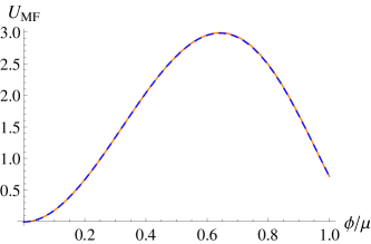
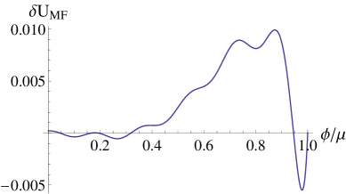
Figure 2: Reproduction of the exact mean field solution in a 10-element harmonic basis (left panel). The error of the reproduction (right panel).

The error is on the percent level: this is the typical error in the calculations also later on.

V.2 Bosonic fluctuations

If we take into account the bosonic fluctuations, ie. we consider the complete set of equations (13), we should follow the strategy described in Section II. First we solve the $\mu=0$ case, ie. (13a) on the ${\cal D}_{>}$ domain. This solution will be true at the outer domain at $\mu\neq 0$, too. In this domain the usual potential expansion approach works, and so we will seek $U_{0}(k,\varphi)$ as a polynomial in $\varphi^{2}$, around an expansion point $v^{2}$:

$$U_{k}(\varphi)=U_{0}+\frac{m_{k}^{2}}{2}(\varphi^{2}-v_{k}^{2})+\frac{\lambda_{k}}{24}(\varphi^{2}-v_{k}^{2})^{2}.$$ (67)

This form makes possible to treat the symmetric and the broken phase together. In the former case we should expand around zero field value, and so $v^{2}=0$; in the latter case $v$ denotes the minimum of the potential, therefore $m^{2}=0$ must be chosen. But we can keep both variable, and only in the course of the solution do we choose the appropriate expansion point.

Expanding (13a) to power series in the variable $\varphi^{2}$ around $v^{2}$, the different orders must separately satisfy the equation. This leads to the differential equations ($\omega_{B}^{2}=k^{2}+m^{2}+\frac{\lambda}{3}v^{2}$ and $\omega_{F}^{2}=k^{2}+g^{2}\varphi^{2}$)

$$\partial_{k}U_{0}-\frac{m^{2}}{2}\partial_{k}v^{2}= \frac{k^{4}}{12\pi^{2}}\left[\frac{1}{\omega_{B}}-\frac{4}{\omega_{F}}\right]$$

$$\frac{\lambda}{6}\partial_{k}v^{2}-\partial_{k}m^{2}= \frac{k^{4}}{12\pi^{2}}\left[\frac{\lambda}{2\omega_{B}^{3}}-\frac{4g^{2}}{\omega_{F}^{3}}\right]$$

$$\partial_{k}\lambda= \frac{3k^{4}}{\pi^{2}}\left[\frac{\lambda^{2}}{16\omega_{B}^{5}}-\frac{g^{4}}{\omega_{F}^{5}}\right].$$ (68)

These equations can be solved. Using the working point (66) we remain in the symmetric phase. The low energy part of the running of the couplings is shown in Fig. 3.

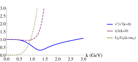
Figure 3: The running of the couplings in the ${\cal D}_{>}$ regime. In the plot the couplings are rescaled in order to show in a single plot.

Having the solution for all $k$ and $\varphi$ we can cut off the boundary conditions with the rule (cf. (21)) $V_{0}(x)=U_{>}(K(x),x)$; this results in the figure Fig. 4.

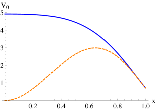
Figure 4: The boundary condition at $\mu=\mu_{MF}$ (solid blue line). To compare, we also plotted the mean field case (dashed orange line).

Starting from this boundary condition we can solve (45). We used ${\cal N}=8$ basis elements, and the inverse square root was expanded to ${\cal P}=0,1,2,3$ and $4$ order. The complete result depends on the choice of the regularizing mass: we played around with its value to find the best convergence, in the present case it was $U^{\prime\prime}(\varphi=\mu)/18$. The resulting curves can be seen on the right panel of Fig. 5, where also the result of mean field analysis is shown.

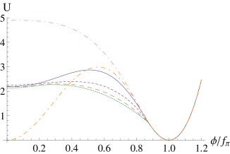
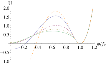
Figure 5: The effective potential resulting from the FRG calculation. The different curves correspond to different order of the expansion of the radiative correction in (45). In the left panel $\mu=\mu_{MF}$ the mean field critical chemical potential, in the right panel $\mu=\mu_{c}=1.053\mu_{MF}$ the true critical chemical potential. In the right panel the ${\cal P}=0$ case is not shown, and the mean field curve goes down to $U_{MF}(\varphi=0)=-2.92$.

The same analysis at a somewhat larger chemical potential ($\mu_{c}=1.053\mu_{MF}$) results the plot on the left panel of Fig. 5: this is the critical chemical potential of the first order phase transition belonging to the given couplings (65) describing the working point (66).

To interpret what we can see in the figures, we recall that the exact effective potential must be convex. Since the boundary condition fixes the value of the potential at the border, if $\mu\leq\mu_{c}$, then the exact effective potential is a constant. So if ${\cal P}\to\infty$ we should find shallower and shallower effective potential until it flattens out completely. This means that we cannot expect pointlike convergence.

In the figures of Fig. 5 one can identify two regimes: at those $\varphi$ values, where the curvature of the potential is positive, we can observe rather good convergence. The change of the effective potential from the mean field (${\cal P}=0$) to the one loop (${\cal P}=1$) approximation is large yet, from ${\cal P}=1$ to ${\cal P}=2$ the change is moderate, but still observable (especially on the right panel). But the potential values of ${\cal P}=2,3,4$ are almost the same, there is a small deviation between them.

In the other regime, where the curvature is negative, the effective potential is concave, we find bad convergence. This can be expected, since the exact result must have a non-negative curvature.

Based on these observations we can treat ${\cal P}=2$ or 3 as the best approximation for the coarse grained effective potential, at least when we interested in the thermodynamics. At those points, where the exact effective potential has positive curvature, these curves already converge to the good values; at those points, where the curvature is negative, the value of the ${\cal P}=2$ or 3 appriximation is irrelevant. We must be aware, however, that quantities like the surface tension can not be reliably calculated from these approximations.

This method provides a very effective and fast approach to calculate the (relevant part of the) exact effective potential. The numerical evaluation of the ${\cal P}=2$ or 3 formula is just seconds, the convergence is very good, the results are rather stable against the actual choice of the number of basis elements, or the exact value of the expansion mass $M^{2}$.

V.3 Phase diagram

In the thermodynamics a particularly interesting question is the order of the phase transition as a function of the coupling constants. One can find a curve $g_{c}(\lambda)$ that is the border line between the first and second order regimes in this model. The goal of this subsection is to find this function.

To understand what happens, we pick up couplings $\lambda,g$, and start from a low chemical potential, where the system is in the broken phase (by construction). The minimum of the potential is at $\varphi=\pm v\neq 0$ (because of the $Z_{2}$ symmetry $\varphi\leftrightarrow-\varphi$), the curvature at $\varphi=0$, denoted by $m_{0}^{2}$, is negative $m_{0}^{2}<0$.

If we start to increase the chemical potential, both $v$ and $|m_{0}^{2}|$ decrease, sooner or later they will cross zero. There are two possibilities: $|m_{0}^{2}|$ reaches zero before $|v|$, or they reach zero in the same time. In this model the $Z_{2}$ symmetry requires zero slope at $\varphi=0$, therefore there is either a minimum or a maximum. For $m_{0}^{2}<0$ it is a maximum, if $m_{0}^{2}=0$ while $v$ still positive, then a new minimum is formed, therefore we have a first order transition later. If $v$ and $m_{0}^{2}$ reach zero in the same time, then we have a second order transition. Therefore we can identify the order of the phase transition observing only the second order derivative at $\varphi=0$ and the position of the minimum (cf. Fig. 6).

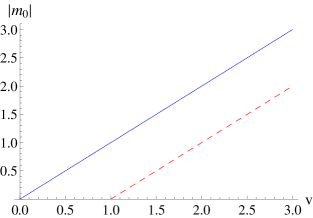
Figure 6: Identification of the order of the phase transition: if the $|m_{0}|$ vs. $v$ curve crosses zero at $v=0$, then we have a second order, if it crosses zero at positive $v$, a first order transition.

Note that in this way at most second order derivatives are needed for the identification of the order of the transition.

In the first order regime the $m_{0}=0$ point is reached at a certain $\mu=\mu_{u}(\lambda,g)$ value, where $v=v_{c}(\lambda,g)$. We can solve the $v_{c}(\lambda,g_{c}(\lambda))=0$ equation to determine the point, where a second order transition first shows up. The resulting $g_{c}(\lambda)$ curve is the borderline of the first and second order regimes. This curve can be determined with the method discussed above for the mean field and for the one loop computation and for the FRG case. The one loop can be accessed from FRG as the first term in the expansion of the inverse square root using the unimproved $\sigma$ mass as the expansion point. In the FRG computation we used a 12-element basis, and second and third order expansion of the inverse square root. The resulting plot can be seen on Fig. 7.

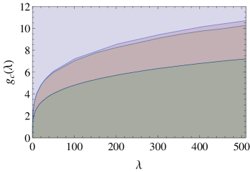
Figure 7: Phase diagram in the coupling constant plane for the scalar Yukawa model. In the darker regimes we have second order, in the lighter regimes first order phase transition. The curves from bottom to top correspond to the mean field, one loop and FRG calculations, respectively. There are coupling pairs, where mean field predicts first order transition, but according to the FRG calculation it is still second order.

As we see, at small Yukawa couplings the phase transition is second order, while for large Yukawa couplings it is first order. In the plot the darker regions denote second, the lighter the first order regime. The borderline of the two regimes depend on the order of the approximation: the mean field calculation (ie. tree level approximation for bosons) predicts the strongest phase transition, in the sense that for increasing $g$ in this approximation comes the first order regime earliest. So there is a regime, where the mean field already predicts first order phase transition, but the exact result is still a second order one. The one loop approximation is already fairly good, it predicts only slightly stronger phase transition than the exact result. These results are in accord with observations in other models Herbst:2013ail ; Jakovac:2003ar .

We remark that all phase boundaries can be well fitted by a

$$g_{c}(\lambda)\approx C\lambda^{1/4}$$ (69)

analytic curve. The reason for this good fit is that if the effective potential is analytic around $\varphi=0$, then we can power expand it around $\varphi=v$ for small enough vacuum expectation value:

$$U(\varphi)=A(\varphi^{2}-v^{2})^{2}+B(\varphi^{2}-v^{2})^{3}+\dots.$$ (70)

If $A>0$ while $v\to 0$ then it is a second order transition, if $A<0$ while $v\to 0$, this describes a first order transition, at the border line $A=0$. Perturbative arguments dictate an expansion in the couplings as

$$A=A_{1}\lambda+A_{2}\lambda^{2}+A_{3}\lambda^{3}-A_{4}g^{4}+\dots$$ (71)

with some coefficients. This can be made vanish for small $\lambda$ and $g$ by the assumption $A_{1}\lambda\approx A_{4}g^{4}+{\cal O}(g^{6})$. This argumentation, although perturbative, seems to be remain valid even in the domain of stronger couplings, too. The coefficient in the $g_{c}(\lambda)\sim\lambda^{1/4}$ relation already depends on the level of approximation, but converges nicely: the ratio of the mean field and the exact result is about $\sim 1.45$, for the ration of the one loop and mean field results it is only $\sim 1.04$.

Fig. 8 serves to demonstrate the convergence at larger orders. As we see, the relative deviation of the the second and third order expansion of the square root is $0.2$-$1.2\%$, these yields curves within line width in Fig. 7. This supports also our earlier finding, that in the physically sensible regime the second order expansion of the inverse square root is already close enough to the exact one, provided we use an appropriate expansion point.

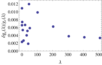
Figure 8: Relative difference of the border line using second or third order expansion of the inverse square root. The difference is below 1.5%, which hints for a good convergence.

VI Conclusions

In this paper we proposed a systematic approximation scheme for the treatment of the FRG equations at finite chemical potential. In short, the Fermi surface divides the available $(k,\varphi)$ domain into two parts: in the high energy ${\cal D}_{>}$ domain the vacuum equations are valid, while in the small energy ${\cal D}_{<}$ regime the statistical fluctuations of the fermionic modes are also present. Starting from initial condition posed at $k=\Lambda$, in the ${\cal D}_{>}$ domain the solution is not affected by the presence of the Fermi surface. This solution, on the other hand, provides a boundary condition for the equation in the ${\cal D}_{<}$ domain. To be able to solve the equations in the ${\cal D}_{<}$ domain, we introduced new variables ($x$ and $y$), with them we transformed the Fermi-surface into a rectangle. After separating the boundary conditions we had to solve an inhomogeneous nonlinear partial differential equation in this rectangle with zero boundary conditions. We looked for the solution in a form of a series in a complete basis of harmonic functions, then for the coefficients we had a set of ordinary differential equations. We performed another expansion, namely we expanded the $\sim(k^{2}+u^{\prime\prime})^{-1/2}$ type term in powers of $(u^{\prime\prime}-M^{2})^{n}$, where $M^{2}$ was an appropriately chosen mass.

Having two expansions (the number of basis elements, and the order of the expansion of the inverse square root), we had to study the convergence in both. As it turned out, a moderate number of basis elements (6-12) is enough to have a good convergence. The order of the expansion of the square root is a more delicate question. As we have argued in the paper, the exact effective potential should be convex, unlike the physically more useful coarse grained effective potential. What we really need is the convergence in the regimes, where the potential is convex, in the unphysical, concave parts we can not expect good convergence properties. The convergence in the convex part of the effective potential can be achieved (by a proper choice of the expansion point $M^{2}$), already by taking into account a second or third order expansion of the inverse square root (corresponding to a linear or quadratic power of $(u^{\prime\prime}-M^{2})$).

This method is a semi-analytic approach to the solution of the FRG equations at finite chemical potential, similar to the polynomial expansion used at zero chemical potential. It is a powerful and accurate method, the differential equations for the evolution of the coefficients in the harmonic basis are well conditioned (unlike in the expansion in polynomial basis), so the numerical treatment is easily accessible and fast.

With this method we determined the phase structure of the Yukawa model, ie. we determined the line in the coupling constant plane, where the boundary between the first and second order phase transitions is situated. One can compare the results of the different approximations (mean field, one loop, exact). The main result from this study is that the bosonic fluctuations soften the strength of the transition, making it more “second-order-like”. More precisely, there is a region in the coupling constant plane, where the mean field calculation predicts a first order transition, but in fact it is a second order transition according to the exact result. In this sense the mean field predicts the strongest phase transition, then the one loop approximation follows, the exact result gives the weakest transition.

As a future prospect, this method can be applied to other models where the small temperature, finite chemical potential regime is physically significant. Moreover, as we also mentioned in the paper, there is a natural expansion towards the finite temperature and finite chemical potential regime.

References

- (1) for a review see: H. Gies, Lect. Notes Phys. 852, 287 (2012) [hep-ph/0611146].
- (2) T. K. Herbst, J. M. Pawlowski and B. J. Schaefer, Phys. Rev. D 88, no. 1, 014007 (2013) doi:10.1103/PhysRevD.88.014007 [arXiv:1302.1426 [hep-ph]].
- (3) M. Drews, T. Hell, B. Klein and W. Weise, Phys. Rev. D 88 (2013) 9, 096011 doi:10.1103/PhysRevD.88.096011 [arXiv:1308.5596 [hep-ph]].
- (4) M. Drews and W. Weise, Phys. Lett. B 738, 187 (2014) doi:10.1016/j.physletb.2014.09.051 [arXiv:1404.0882 [nucl-th]].
- (5) M. Drews and W. Weise, Phys. Rev. C 91, no. 3, 035802 (2015) doi:10.1103/PhysRevC.91.035802 [arXiv:1412.7655 [nucl-th]].
- (6) P. Pósfay, G. G. Barnaföldi and A. Jakovác, arXiv:1510.04906 [hep-ph].
- (7) J. Eser, M. Grahl and D. H. Rischke, Phys. Rev. D 92, no. 9, 096008 (2015) doi:10.1103/PhysRevD.92.096008 [arXiv:1508.06928 [hep-ph]].
- (8) C. Wetterich, Nucl. Phys. B 352, 529 (1991).
- (9) C. Wetterich, Phys. Lett. B 301, 90 (1993).
- (10) I. Nandori, JHEP 1304, 150 (2013) doi:10.1007/JHEP04(2013)150 [arXiv:1208.5021 [hep-th]].
- (11) D. F. Litim, Phys. Rev. D 64, 105007 (2001) doi:10.1103/PhysRevD.64.105007 [hep-th/0103195].
- (12) A. Jakovác, A. Patkós and P. Pósfay, Eur. Phys. J. C 75, no. 1, 2 (2015) doi:10.1140/epjc/s10052-014-3228-1 [arXiv:1406.3195 [hep-th]].
- (13) P. Mati, Phys. Rev. D 91, no. 12, 125038 (2015) doi:10.1103/PhysRevD.91.125038 [arXiv:1501.00211 [hep-th]].
- (14) J. A. Adams, J. Berges, S. Bornholdt, F. Freire, N. Tetradis and C. Wetterich, Mod. Phys. Lett. A 10, 2367 (1995) doi:10.1142/S0217732395002520 [hep-th/9507093].
- (15) K. Fukushima, K. Kamikado and B. Klein, Phys. Rev. D 83, 116005 (2011) doi:10.1103/PhysRevD.83.116005 [arXiv:1010.6226 [hep-ph]].
- (16) D. F. Litim, J. M. Pawlowski and L. Vergara, hep-th/0602140.
- (17) A. Schmitt, Lect.Notes Phys.811:1-111,2010 [arXiv:1001.3294]
- (18) Norman K. Glendenning, Compact stars : nuclear physics, particle physics, and general relativity 2nd ed. (New York ; London : Springer, c2000.)
- (19) A. Jakovac, A. Patkos, Z. Szep and P. Szepfalusy, Phys. Lett. B 582, 179 (2004) doi:10.1016/j.physletb.2004.01.008 [hep-ph/0312088].
- (20) J. Borchardt and B. Knorr, Phys. Rev. D 91, no. 10, 105011 (2015) doi:10.1103/PhysRevD.91.105011 [arXiv:1502.07511 [hep-th]].
- (21) J. Borchardt, H. Gies and R. Sondenheimer, arXiv:1603.05861 [hep-ph].
- (22) J. Borchardt and B. Knorr, arXiv:1603.06726 [hep-th].