Identifying two-dimensional $Z_{2}$ antiferromagnetic topological insulators

Abstract

We revisit the question of whether a two-dimensional topological insulator may arise in a commensurate Néel antiferromagnet, where staggered magnetization breaks both the elementary translation and time reversal, but retains their product as a symmetry. In contrast to the so-called $Z_{2}$ topological insulators, an exhaustive characterization of antiferromagnetic topological phases with the help of a topological invariant has been missing. We analyze a simple model of an antiferromagnetic topological insulator and chart its phase diagram based on a recently proposed criterion for centrosymmetric systems [Fang et al., Phys. Rev. B 88, 085406 (2013)]. We then adapt two methods, originally designed for paramagnetic systems, and make antiferromagnetic topological phases manifest. The proposed methods apply far beyond the particular example treated in this work, and admit straightforward generalization. We illustrate this by considering a non-centrosymmetric system, where there are no simple criteria to identify topological phases. We also present an explicit construction of edge states in an antiferromagnetic topological insulator.

I Introduction

Topological states of matter have become a focus of much theoretical and experimental effort (see [Hasan and Kane, 2010; Qi and Zhang, 2011] for detailed reviews, and [Kane and Mele, 2005a, b; Xu and Moore, 2006; Wu et al., 2006] for some of the earlier work on the subject). Such an interest is dictated by a remarkable stability of topological phases and of their physical properties with respect to perturbation.

Topological insulators (TIs) provide a simple example of such phases in a non-interacting system. From a band structure textbook perspective, these are ordinary band insulators with a spectral gap. However, in addition to the mere presence of the gap, the bands may have a non-trivial reciprocal-space topology, that manifests itself, inter alia, by the presence of surface states, stable against moderate bulk and surface perturbations. This topology may be encapsulated in a special quantum number, assigned to the occupied bulk bands: insulators with an odd value of this number have protected gapless surface states within the bulk gap, and are called “topological”. For an even value of this number, surface states within the bulk gap are not protected; such insulators are called “topologically trivial”. Switching between an even and an odd value requires closing of the bulk gap and a phase transition; otherwise, a smooth variation of the Hamiltonian leaves this number intact. Hence it is called a $Z_{2}$ (“even-odd”) topological invariant.

Symmetry tends to facilitate description, thus it is not surprising that some of the pioneering work on topological insulators studied rather symmetric systems: notably those symmetric with respect to both the time reversal $\theta$ and inversion $I$. Simultaneous presence of these two symmetries guarantees double degeneracy of bulk Bloch eigenstates at any momentum in the Brillouin zone. For two-dimensional models, one of the better-known examples of this kind is the so-called Bernevig-Hughes-Zhang (BHZ) model Bernevig et al. (2006), that we briefly review in this article. Bulk Bloch eigenstates may also be degenerate in systems with more delicate symmetries. A convenient example is provided by a collinear Néel antiferromagnet, sketched in the Fig. 1, where the time reversal symmetry $\theta$ is explicitly broken by magnetic order. Black and white circles in the figure depict the two sublattices of a square-lattice Néel antiferromagnet, and correspond to the opposite directions of local magnetization. Both the time reversal $\theta$ and a translation $T_{\bf a}$ by half a period ${\bf a}$ invert the local magnetization (interchange black and white circles in the Fig. 1, and thus none of them is a symmetry of the system. However, the product $\theta T_{\bf a}$ remains a symmetry and conspires with inversion $I$ to ensure the double degeneracy of Bloch eigenstates at any momentum in the Brillouin zone – the same way as, in paramagnetic insulator, such a degeneracy appears due to a conspiracy of $\theta$ and $I$.

With this similarity in mind, one may inquire whether an antiferromagnet may host a topologically non-trivial state of matter such as a topological insulator and, if so, whether the latter may have properties distinguishing it from its non-magnetic counterparts. Several pioneering studies have already addressed this issue. In particular, Mong et al. Mong et al. (2010) have posed the question of whether an antiferromagnetic insulator may be topologically non-trivial, and whether or not it may be characterized by a topological invariant. The authors concluded that, in contrast to non-magnetic insulators, the presence of surface states in an antiferromagnet is sensitive to whether the surface is symmetric under the same combination of a translation and time reversal as the bulk. This result was obtained for three-dimensional materials and was confirmed for a special choice of boundary. The investigation of three-dimensional antiferromagnetic topological insulators has, since then, become an extensive subject of study. Liu (2013); Zhang and Liu (2015); Liu et al. (2014); Fang and Fu (2015); Fang et al. (2013)

In a subsequent publication, Fang et al. Fang et al. (2013) studied a class of systems that, beyond symmetries involving time reversal, also possess an inversion center. They argued that antiferromagnetic insulators with such properties may be characterized by a $Z_{2}$ topological invariant that, similarly to a paramagnet, involves the product of parity eigenvalues over a set of special points in the Brillouin zone. However, in an antiferromagnet this set of special points would comprise only a half of the points that are relevant in the paramagnetic case.

The systems mentioned above can be viewed as a particular example of the so-called crystalline topological insulators, which have been studied in 3 dimensions Fu (2011); Kargarian and Fiete (2013); Liu et al. (2013); Serbyn and Fu (2014); Liu et al. (2014); Zhang and Liu (2015); Fang and Fu (2015) and also in the case of the two-dimensional honeycomb lattice Jadaun et al. (2013). The key ingredient of all these studies is the presence of time reversal symmetry supplemented by a crystal symmetry.

Here, we study the precise form of this $Z_{2}$ invariant in an antiferromagnetic insulator for a particular generalization of the BHZ model Bernevig et al. (2006) in two dimensions. In the Sec.II we briefly review the BHZ model and its symmetries. We then extend the model by turning on staggered magnetization, identify its symmetries and ask whether its topology may be characterized similarly to how it is done for the paramagnetic BHZ model. In the Sec.III, we review some of the methods used to study topological insulators: the Fu-Kane topological invariant Fu and Kane (2007), the parallel transport method Soluyanov and Vanderbilt (2012), the method of Wannier Charge Centers King-Smith and Vanderbilt (1993); Yu et al. (2011) – and, finally, an explicit construction of edge states. We show that these methods do not apply to an antiferromagnet verbatim, and show how they must be adapted. The model we consider is centrosymmetric, hence we test our results against the $Z_{2}$ topological invariant in the form proposed by Fang et al., and find perfect agreement. However, our adaptation of the Wannier Charge Center method applies perfectly well even when the parity-based criterion no longer does. To illustrate this, in the Sec. (IV) we consider a non-centrosymmetric perturbation of the initial Hamiltonian: the method successfully identifies the topological phases. Finally, the Sec. V contains concluding remarks and an outlook.

II The BHZ model and its extension to antiferromagnetism

Bernevig, Hughes and Zhang proposed a model to describe topological insulating phases in HgTe/CdTe quantum wells. Bernevig et al. (2006) In this section, we first present the Hamiltonian they introduced. We then see how it is modified in the presence of antiferromagnetism, and study how magnetic order affects its topological properties.

II.1 The BHZ model

We consider a square lattice, defined by lattice vectors $\mathbf{R}=pa\hat{\mathbf{X}}+qa\hat{\mathbf{Y}}$, with $p,q\in\mathbb{Z}$ (see the Fig. 1). A unit cell labelled by $\mathbf{R}$ hosts four single-electron states, $|\mathbf{R},n\rangle$: two $s$-type orbitals, $|\uparrow,s\rangle$ and $|\downarrow,s\rangle$, and two $p$-type orbitals, $|\uparrow,p_{x}+ip_{y}\rangle$ and $|\downarrow,p_{x}-ip_{y}\rangle$.

We will use the index $\nu$ to denote the $s$-state ($\nu=+$) or a $p$-state ($\nu=-$), and $\sigma$ for the spin. In this basis, the BHZ Hamiltonian may be written as:

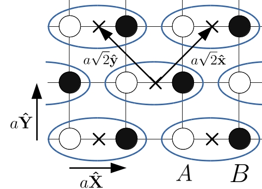
Figure 1: (color online) Square lattice, on which the Hamiltonian is defined. In the absence of a staggered magnetic field, the primitive Bravais lattice vectors are $a\mathbf{\hat{X}}$ and $a\mathbf{\hat{Y}}$. In the presence of staggered magnetization, the dimerized lattice is defined by the primitive vectors $a\sqrt{2}\mathbf{\hat{x}}$ and $a\sqrt{2}\mathbf{\hat{y}}$. In this case, a unit cell (in blue) comprises two sites, A and B (white and black dots, respectively). The center of a unit cell (denoted $\mathbf{r}$ in the main text) is represented by a cross.

$$\mathcal{H}_{BHZ} =\sum_{\mathbf{R},\sigma,\nu}(\mu+\nu\Delta\mu)c_{\sigma,\nu}^{\dagger}(\mathbf{R})c_{\sigma,\nu}(\mathbf{R})$$

$$+\sum_{<\mathbf{R},\mathbf{R^{\prime}}>,\sigma,\nu}(t+\nu\Delta t)(c_{\sigma,\nu}^{\dagger}(\mathbf{R})c_{\sigma,\nu}(\mathbf{R^{\prime}})+h.c)$$

$$+\sum_{\mathbf{R},\sigma,\nu}-i\alpha\sigma(c_{\sigma,\nu}^{\dagger}(\mathbf{R}+a{\bf\hat{X}})c_{\sigma,-\nu}(\mathbf{R})-h.c)$$

$$+\sum_{\mathbf{R},\sigma,\nu}\alpha\nu(c_{\sigma,\nu}^{\dagger}(\mathbf{R}+a{\bf\hat{Y}})c_{\sigma,-\nu}(\mathbf{R})+h.c).$$ (1)

The first term ($\mu_{\pm}=\mu\pm\Delta\mu$) originates from the energy difference of the the s- and p-symmetric orbitals. The second term corresponds to the nearest-neighbor hopping between the same orbitals, with different hopping amplitudes, $t_{\pm}=t\pm\Delta t$. Finally, the remaining two terms hybridize the two species via the amplitude $\alpha$, and are of spin-orbital nature.

The Hamiltonian is non-interacting, and its ground state is built by filling the single-electron states up to the Fermi energy. At half-filling, the bulk spectrum has an insulating gap. However, depending on the Hamiltonian parameters, the system may be a trivial or a topological insulator, in the sense described in the Introduction – as we argue below. It turns out that the trivial phase is realized for $|\Delta\mu|>4|\Delta t|$: a boundary of such a system hosts an even number of pairs of edge states. By contrast, when $|\Delta\mu|<4|\Delta t|$, the system is in a topological phase, and has an odd number of pairs of states at the boundary. Thus, in the topological phase, at least a single pair of chiral edge states is guaranteed to exist. Transition from a topological to the trivial state implies closing the band gap (here, this occurs at $|\Delta\mu|=4|\Delta t|$) and is a quantum phase transition. Hence the term “topologically protected edge states”. Topology of either of the phases can be characterized by the parity of the number of pairs of edge states, which, as we will see below, is related to the $Z_{2}$ topological invariant.

It is interesting to note that the strength $\alpha$ of the spin-orbit coupling does not appear in the above inequalities despite being responsible for the existence of the insulating gap.

Translational invariance of the crystal lattice allows one to define the Bloch Hamiltonian

$$H_{BHZ}(\mathbf{k})=e^{-i\mathbf{k}\cdot\hat{\mathbf{R}}}\mathcal{H}_{BHZ}e^{i\mathbf{k}\cdot\hat{\mathbf{R}}}$$ (2)

and obtain

$$H_{BHZ}(\mathbf{k}) =\mu+2t\cos(ak_{X})+2t\cos(ak_{Y})$$

$$\ +(\Delta\mu+2\Delta t\cos(ak_{X})+2\Delta t\cos(ak_{Y}))\tau^{z}$$

$$\ -2\alpha\sin(ak_{X})s^{z}\tau^{x}+2\alpha\sin(ak_{Y})\tau^{y},$$ (3)

where the $s^{a}$ and $\tau^{b}$, with $a$ and $b$ standing for $x,~{}y$ and $z$, are the Pauli matrices acting in the spin and orbital spaces, respectively. The identity operator in either of the two spaces is omitted for brevity: for example, the last term in the Eq.(II.1) acts as the identity operator in the spin space.

The BHZ Hamiltonian is invariant under the time reversal $\Theta=is^{y}K$, where $K$ is complex conjugation. The operator $\Theta$ is anti-unitary, and $\Theta^{2}=-1$.

Using the Kramers theorem arguments, one can show that the eigenstates of the BHZ Hamiltonian come in Kramers pairs (see appendix B for a general proof), a state at momentum $\mathbf{k}$ being related to its degenerate counterpart at momentum $\mathbf{-k}$. This has an important consequence for a set of special points $\Gamma_{i}=(\Gamma^{x},\Gamma^{y})$ in the Brillouin zone, called time reversal invariant momenta (TRIM). These special points satisfy the equality $-\Gamma_{i}=\Gamma_{i}+\mathbf{G}$, where $\mathbf{G}$ is a reciprocal lattice vector, and $\Gamma^{x},\Gamma^{y}$ take values $0$ or $\pi/a$. As $\Gamma_{i}$ is equivalent to $-\Gamma_{i}$, the TRIM states are doubly degenerate, an important property that we will use later.

The Hamiltonian is also invariant under inversion $\mathcal{P}=\sum_{\mathbf{R}}\tau_{z}|-\mathbf{R}\rangle\langle\mathbf{R}|$ (the $\tau_{z}$ comes from the fact that the s-orbital remains invariant under inversion, while the p-orbital acquires a minus sign). Note that $\mathcal{P}H(\mathbf{k})\mathcal{P}^{-1}=H(\mathbf{-k})$ and $\mathcal{P}^{2}=1$.

Combining the $\Theta$ and $\mathcal{P}$, one can show that each Bloch eigenstate also has a degenerate partner at the same momentum.

II.2 Generalization to a staggered magnetization

Looking to study the effect of anti-ferromagnetism on topological insulators, we introduce a staggered magnetization, following the Refs. [Kulikov and Tugushev, 1984; Ramazashvili, 2008, 2009; Fang et al., 2013; Guo et al., 2011], via the term:

$$\sum_{\mathbf{R},\sigma,\nu}(-1)^{\mathbf{R}}\sigma m\ c_{\sigma,\nu}^{\dagger}(\mathbf{R})c_{\sigma,\nu}(\mathbf{R}),$$ (4)

where the $m$ is the product of the antiferromagnetic ordered moment and the constant that couples it to the conduction electron spin. The Eq.(4) introduces antiferromagnetic order phenomenologically, independently of the precise form of the interaction that gives rise to magnetism. At the same time, it entirely neglects both thermal and quantum fluctuations of the magnetic order. This may be justified for the ordered moment that is noticeable on the scale of the Bohr magneton, and at temperatures well below the Néel temperature.

Staggered magnetization in the Eq.(4) doubles the unit cell of the paramagnetic state and reduces its translation symmetry. The new Bravais lattice is now defined by the vectors $\mathbf{r}=pa\sqrt{2}\hat{\mathbf{x}}+qa\sqrt{2}\hat{\mathbf{y}},p,q\in\mathbb{Z}$, and contains two sites per unit cell, A and B, positioned at $\mathbf{R}_{A}=\mathbf{r}-\frac{a}{2}\hat{\mathbf{X}}$ and $\mathbf{R}_{B}=\mathbf{r}+\frac{a}{2}\hat{\mathbf{X}}$ respectively (see the Fig. 1). Hereafter we set $a=\frac{1}{\sqrt{2}}$. The unitcell of lattice vector $\mathbf{r}$ now possesses eight states, $|\mathbf{r},n\rangle$.

We define the Bloch Hamiltonian with staggered magnetization as:

$$H(\mathbf{k})=e^{-i\mathbf{k}\cdot\hat{\mathbf{r}}}\mathcal{H}e^{i\mathbf{k}\cdot\hat{\mathbf{r}}}.$$ (5)

One may note the difference between the Eqs.(2) and (5). Here, in contrast to the choice made by Guo et al., the real positions of the sites, $\mathbf{R}_{A}$ and $\mathbf{R}_{B}$, have been replaced by the position $\mathbf{r}$ of the center of the unit cell to which the sites belong. This choice in the definition of the Bloch Hamiltonian ensures $H(\mathbf{k}+\mathbf{G})=H(\mathbf{k})$ for any reciprocal lattice vector $\mathbf{G}$Fruchart et al. (2014), a property that will prove useful later, as we wish to define quantities that are continuous over the BZ torus. We obtain:

$$H(\mathbf{k}) =\mu+\Delta\mu\tau^{z}+ms^{z}\sigma^{z}$$

$$+(2C_{-}^{2}+2C_{-}C_{+})(t\sigma^{x}+\Delta t\tau^{z}\sigma^{x})$$

$$+(2C_{-}S_{-}+2C_{+}S_{-})(t\sigma^{y}+\Delta t\tau^{z}\sigma^{y})$$

$$-2\alpha S_{-}(C_{-}s^{z}\tau^{x}\sigma^{x}+S_{-}s^{z}\tau^{x}\sigma^{y})$$

$$+2\alpha S_{+}(C_{-}\tau^{y}\sigma^{x}+S_{-}\tau^{y}\sigma^{y})$$

where $C_{\pm}\equiv\cos\left[(k_{x}\pm k_{y})/2\right]$ and $S_{\pm}\equiv\sin\left[(k_{x}\pm k_{y})/2\right]$, while $\sigma$, $s$ and $\tau$ are the Pauli matrices acting in the sub-lattice (A and B), spin and orbital spaces, respectively.

The time reversal and the elementary translation both invert the local magnetization, thus none of them is a symmetry of the antiferromagnetic state. However, their product $\Theta_{AF}=T\Theta$ ($T$ being the translation by a vector $a\hat{\mathbf{X}}$) remains a symmetry.

The $\Theta_{AF}$ is also anti-unitary but does not square to $-1$ for an arbitrary momentum in the Brillouin zone. Indeed, as the time reversal operator commutes with any purely spatial transformation, it commutes with any translation, and thus $\Theta_{AF}^{2}=-T^{2}$. One may note that $T^{2}$ is a symmetry of the antiferromagnetic state and acts on a state $|\Psi_{n,\mathbf{k}}\rangle$ as per $T^{2}|\Psi_{n,\mathbf{k}}\rangle=e^{-i2a\mathbf{k}\cdot\hat{\mathbf{X}}}|\Psi_{n,\mathbf{k}}\rangle$. As a result, at certain points in the BZ ($k_{X}=\pi/(2a)~{}mod~{}\pi/a$) the $\Theta_{AF}^{2}$ acts as the identity, which is an obstacle to the definition of Kramers pairs (see the Fig. 2).

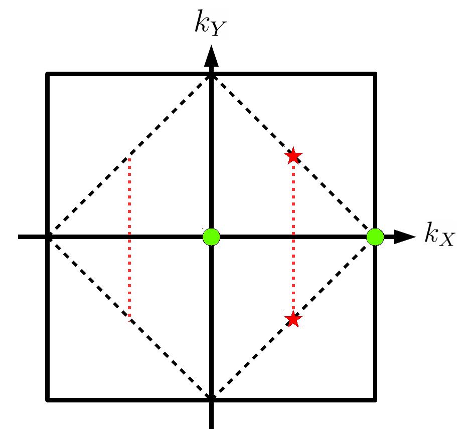
Figure 2: (color online) The big solid black square depicts the paramagnetic Brillouin Zone. It is reduced to the antiferromagnetic Brillouin Zone (black dashed square) in the presence of the staggered magnetization. The red dotted lines correspond to points in the antiferromagnetic Brillouin Zone, where $\Theta_{AF}^{2}=1$. They have no horizontal counterparts since the chosen $\Theta_{AF}$ involves translation only along the $x$-axis. The two red stars denote the two A-TRIM, where $\Theta_{AF}^{2}=1$, while the green circles correspond to the B-TRIM, where $\Theta_{AF}^{2}=-1$.

However, the system is still invariant under the inversion symmetry, represented by the operator $\mathcal{P}_{AF}$, whose expression is given in the Appendix B.

Thanks to both symmetries, one may show that it is still possible to separate the states in Kramers-like pairs relating a state of momentum $\mathbf{k}$ to a state of momentum $\mathbf{-k}$ (see Appendix B). This will prove indispensable in the next section, when computing the $Z_{2}$ invariant in the antiferromagnetic case. Moreover, one may show that the combined symmetry $\mathcal{P}_{AF}\Theta_{AF}$ is anti-unitary and squares to $-1$. Thus, each Bloch eigenstate possesses an orthogonal degenerate partner at the same momentum, and the bulk bands are doubly degenerate. Ramazashvili (2008, 2009)

As before, the system has a insulating gap at half-filling, and two questions arise:

• Does a topological phase survive for a finite value of the staggered magnetization?

• Starting from a trivial phase with $m=0$, can we obtain a topological phase by switching on a staggered magnetization?

Fang and collaborators Fang et al. (2013) proposed an expression for the $Z_{2}$ invariant for a two-dimensional Néel antiferromagnet, symmetric under both the $\Theta_{AF}$ and $\mathcal{P}_{AF}$. We will discuss this criterion in more detail in the next section (see the Eq.(17)).

Applied to the case at hand, the criterion due to Fang et al. as expressed by the Eq. (17) suggests the positive answer to both questions. Indeed, e.g. for $\alpha=2$, $t_{+}=3$ and $t_{-}=1$, we obtain the phase diagram in the Fig. 3, where the filled region corresponds to values of $m$ and $\Delta\mu$ where we have a topological insulator (all of the numerical results presented in this article will assume those values for $t_{+}$ and $t_{-}$). The phase diagram shows that, starting in the topological phase at $m=0$ and upon increasing $m$, the system remains non-trivial until $m=\Delta\mu$. On the other hand, if one starts in a trivial phase at $m=0$, there is a range of $m$, where the system becomes topologically non-trivial, corresponding to regions where $|m|<|\Delta\mu|$ and $2|\Delta\mu|<\sqrt{m^{2}+16t_{+}^{2}}+\sqrt{m^{2}+16t_{-}^{2}}$. We verified this by applying the method detailed in the next section to several sets of parameters. The results were in perfect agreement with the prediction of Fang and collaborators.

Because of the staggered magnetization, we are now working with a 8-band model, and once again, the symmetries protect doubly-degenerate bands. Thus, it is now possible to open insulating gaps at $1/4$ and $3/4$ filling, that have no equivalent in the BHZ model. It is also interesting to see if we may have topological phases at such fillings. Using the expression (17) due to Fang et al. for the $Z_{2}$ invariant, we obtain the phase diagram in the Fig. 3, which is once again in perfect agreement with our numerical results.

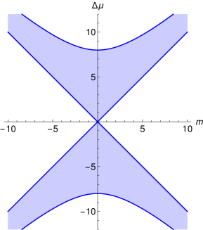
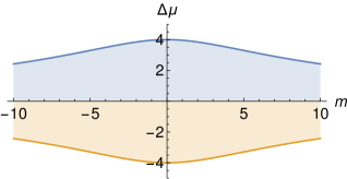
Figure 3: (color online) Phase diagram of the BHZ Hamiltonian of the Eq. (II.1) in the presence of staggered magnetization, for $t_{+}=3$ and $t_{-}=1$. (a) The phase diagram at half-filling. The blue region corresponds to the topological phase. The $m=0$ vertical line corresponds to the phase diagram of the BHZ Hamiltonian. One may notice that a topological phase at $m=0$ survives until a finite threshold value of $m$, and becomes trivial for larger values. Moreover, from the trivial phase at $m=0$, the system may be driven into the topological phase by turning on a staggered magnetization. (b) Overlay of the phase diagrams at 1/4 and 3/4 filling. The blue region corresponds to a topological phase at 1/4 filling, while the yellow region corresponds to a topological phase at 3/4 filling.

III Methods for characterizing topological insulators

In this section we discuss some of the techniques used to characterize time reversal-symmetric topological insulators, using, as an illustration, the BHZ Hamiltonian with and without staggered magnetization.

The first method, due to Fu and Kane Fu and Kane (2006) yields an expression for the $Z_{2}$ invariant that can be computed analytically, knowing continuously defined Bloch functions in the bulk. The second method is an adaptation of the Fu-Kane approach to cases where the Bloch states may be computed only numerically, by studying either the phase variation of Bloch functions across the Brillouin zone Soluyanov and Vanderbilt (2012), or the so-called Wannier charge center trajectories King-Smith and Vanderbilt (1993); Yu et al. (2011). Finally, the third method amounts to an explicit construction of edge states, as the number of edge states may distinguish between the trivial and the topological phase.

III.1 Computation of the Fu-Kane topological invariant

We first present the main steps in the derivation of the $Z_{2}$ topological invariant due to Fu and Kane, and then the modifications necessary to account for the presence of staggered magnetization. The technical details are given in the Appendices A and C.

As the BHZ Hamiltonian enjoys translational invariance, its eigenstates can be written as:

$$|\Psi_{n,\mathbf{k}}\rangle=e^{i\mathbf{k}\cdot\mathbf{r}}|u_{n,\mathbf{k}}\rangle$$ (7)

with $n$ from 1 to 4 for BHZ, and with $|u_{n,\mathbf{k}}\rangle$ being the eigenvectors of the Bloch Hamiltonian of the Eq.(II.1). We choose the $|\Psi_{n,\mathbf{k}}\rangle$ to be continuous over the BZ.

As stated previously, the BHZ Hamiltonian is time reversal-invariant, so the eigenstates of the BHZ Hamiltonian come in Kramers pairs. We can thus separate the eigenstates in $(\{|\Psi_{\mathbf{k},\alpha}^{I}\rangle,|\Psi_{\mathbf{k},\alpha}^{II}\rangle\},\mathbf{k}\in BZ,\alpha=1,2)$, in such a way that

$$|\Psi^{I}_{\alpha,\mathbf{-k}}\rangle = -e^{i\chi_{\mathbf{k},\alpha}}\Theta|\Psi^{II}_{\alpha,\mathbf{k}}\rangle$$

$$|\Psi^{II}_{\alpha,\mathbf{-k}}\rangle = e^{i\chi_{\mathbf{-k},\alpha}}\Theta|\Psi^{I}_{\alpha,\mathbf{k}}\rangle.$$ (8)

The value of the topological invariant will depend on how the phase $\chi$ varies across the BZ.

The topological invariant is defined via the time reversal polarization $P^{\Theta}_{k_{y}}$, introduced by Fu and Kane Fu and Kane (2006) in terms of the center of mass position along $\mathbf{x}$ of hybrid Wannier functions, computed at a fixed $k_{y}$. We define and calculate the $P^{\Theta}_{k_{y}}$ in the Appendix A. The $Z_{2}$ topological invariant may be defined as per

$$\Delta=\sum_{\Gamma^{y}\in\{0,\pi/a\}}P^{\Theta}_{\Gamma^{y}}\ mod\ 2.$$ (9)

As explained in the Ref. [Fu and Kane, 2006], this quantity is a topological invariant, independent of the gauge chosen for the Bloch states.

The topological invariant may be recast in terms of the sewing matrix

$$\mathit{w}(\mathbf{k})_{mn}=\langle\Psi_{m,\mathbf{-k}}|\Theta|\Psi_{n,\mathbf{k}}\rangle~{},$$ (10)

evaluated at the four TRIM as per

$$(-1)^{\Delta}=\prod_{i}\frac{\sqrt{\det[\mathit{w}(\Gamma_{i})]}}{Pf[\mathit{w}(\Gamma_{i})]},$$ (11)

where the index $i$ labels the different TRIM. Even though the above expression appears to rely only on the TRIM states, it has to be computed in a gauge where the eigenstates are defined continuously on the BZ torus.

For a time reversal-symmetric system in the presence of inversion symmetry (which is the case for BHZ Hamiltonian), it turns out that the Eq.(11) admits the form Fu and Kane (2007)

$$(-1)^{\Delta}=\prod_{i=1}^{4}\prod_{\alpha=1}^{N}\xi_{\alpha}(\Gamma_{i})$$ (12)

where $\xi_{\alpha}(\Gamma_{i})=\pm 1$ are the parity eigenvalues of the filled eigenstates $|\Psi^{I}_{\alpha,\Gamma_{i}}\rangle$.

Contrary to the Eq.(11), the expression in the r.h.s of the Eq.(12) has the advantage of relying only on the knowledge of the states at the TRIM. Indeed, $\prod_{\alpha=1}^{N}\xi_{\alpha}(\Gamma_{i})$ is gauge-invariant, so one can compute the $\xi_{\alpha}(\Gamma_{i})$ separately for the different TRIM, without insisting on a continuous definition of the states across the BZ. However, such an expression can be obtained only for a centrosymmetric system.

In the AF case, we doubled the number of bands in the Bloch Hamiltonian – and thus the index $n$, that was defined in the Eq.(7) and took values from 1 to 4, now varies from 1 to 8. As mentioned above, due to the breaking of the time-reversal symmetry, we are no longer guaranteed Kramers degeneracy all over the BZ. Indeed, there is a line $k_{x}-k_{y}=\pm\pi$ of states in the BZ, where $\Theta_{AF}^{2}=1$ and, strictly speaking, the Kramers theorem does not hold. However, thanks to the inversion symmetry, we can recover the degeneracy necessary to write an equivalent of the Eq.(III.1):

$$|\Psi^{I}_{\alpha,\mathbf{-k}}\rangle = -e^{i\chi_{\mathbf{k},\alpha}}e^{i\Phi_{\mathbf{k}}/2}\Theta_{AF}|\Psi^{II}_{\alpha,\mathbf{k}}\rangle$$

$$|\Psi^{II}_{\alpha,\mathbf{-k}}\rangle = e^{i\chi_{\mathbf{-k},\alpha}}e^{-i\Phi_{-\mathbf{k}}/2}\Theta_{AF}|\Psi^{I}_{\alpha,\mathbf{k}}\rangle$$ (13)

for $\alpha=1...4$, and where $\Phi_{\mathbf{k}}$ is defined so that

$$\Theta_{AF}^{2}=-\sum_{\mathbf{k}}e^{i\Phi_{\mathbf{k}}}|\mathbf{k}\rangle\langle\mathbf{k}|.$$ (14)

As above, we define the topological invariant via the time reversal polarization as per the Eq.(9). However, in an antiferromagnet this expression cannot be reduced to a simple form as in the Eq.(11): indeed, the sewing matrix

$$\tilde{\mathit{w}}_{k_{b}}(k_{a})_{mn}=\langle\Psi_{m,\mathbf{-k}}|\Theta_{AF}|\Psi_{n,\mathbf{k}}\rangle.$$ (15)

is no longer anti-symmetric at all the TRIM. In fact, at those TRIM, where $\Theta_{AF}^{2}=1$, that we refer to as A-TRIM in Fig. 2, the Pfaffian in the Eq.(11) cannot even be defined.

However, the topological invariant $\Delta$ of the Eq.(9) may be recast in a form that, albeit less elegant, remains valid in the case of the AF order, for a continuous gauge and under the convenient choice of axes $\mathbf{a}=\mathbf{x}$ and $\mathbf{b}=\mathbf{x}-\mathbf{y}$ described in the appendix C :

$$\Delta=\sum\limits_{\Gamma^{b}\in\{0,\pi\}} \bigg{[} \frac{1}{2\pi i}\int_{0}^{\pi}dk_{a}\nabla_{k_{a}}\text{log\ det}[\tilde{\mathit{w}}_{\Gamma_{b}}(k_{a})]$$ (16)

$$+ \frac{1}{\pi}\sum_{\alpha}(\chi_{\alpha,0,\Gamma_{b}}+\chi_{\alpha,\pi,\Gamma_{b}})\bigg{]}\mathrm{mod}~{}2$$

This expression has the advantage of depending only on $\chi$, and of being computable given a continuous set of Bloch states. It justifies the computation of the following section. Fang et al. proposed an expression for the topological invariant, similar to the Eq. (12):

$$(-1)^{\Delta}=\prod_{\Gamma_{i}\in B-TRIM}\prod_{\alpha=1}^{N}\xi_{\alpha}(\Gamma_{i})$$ (17)

where the B-TRIM are those where $\Theta_{AF}^{2}=-1$. The Eq.(17) does not directly follow from the definition (9) in terms of time-reversal polarization, but is equivalent to our result (16) if there is no band inversion at a single A-TRIM (which is true in the case at hand).

III.2 Parallel Transport Method

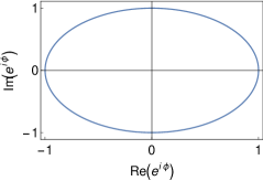
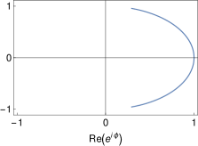
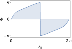
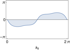
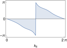
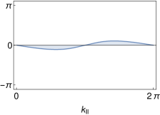
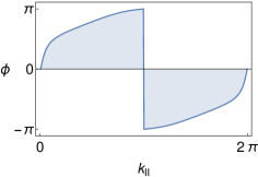
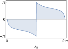
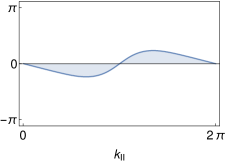
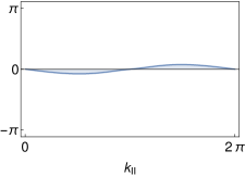
Figure 4: (color online) Results of the parallel transport method for $\Delta\mu=3$. For the two first lines $m=2$ and for the two last lines $m=5$. Each column corresponds to the study of a pair of degenerate bands. From left to right we go from the lower to the higher energy bands. In line 1 and 3, $e^{i\phi}$ is plotted in the complex plane as a parametric function of $k_{\parallel}$. In line 2 and 3, $\phi$ is plotted as a function of $k_{\parallel}$. These plots and the Eq.(21) allow us to evaluate the $Z_{2}$ topological invariant. In both cases, the system is a trivial insulator at 3/4 filling, and a topological insulator at 1/4 filling. At half filling, the system is in the topological phase for $m=2$ and in the trivial phase for $m=5$.

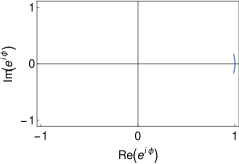
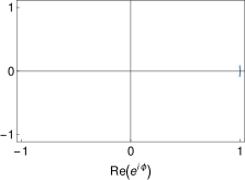
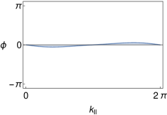
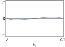
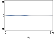
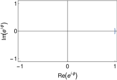
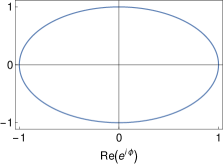
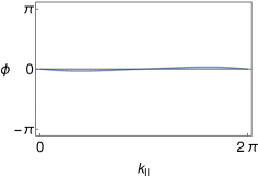
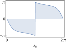
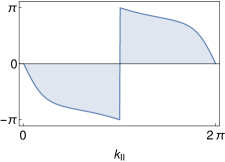
Figure 5: (color online) Same as the Fig. 4 but for $\Delta\mu=9$. We have again $m=2$ for the two first lines and $m=5$ for the two last lines. Each column corresponds to the study of a pair of degenerate bands. In both cases, the system is a trivial insulator at 1/4 and 3/4 filling. At half filling, the system is in the trivial phase for $m=2$ and in the topological phase for $m=5$.

In this section we describe another method, proposed by Soluyanov and Vanderbildt, Soluyanov and Vanderbilt (2012) for computing the topological invariant $\Delta$, which turns out to be efficient for numerical identification of the topological phases in an antiferromagnet.

For time reversal symmetric topological insulators, the latter approach involves enforcing a constraint, setting the relative phase $\chi$ to zero. Eq.(III.1) is thus replaced by:

$$|\tilde{\Psi}^{I}_{\alpha,\mathbf{-k}}\rangle = -\Theta|\tilde{\Psi}^{II}_{\alpha,\mathbf{k}}\rangle$$

$$|\tilde{\Psi}^{II}_{\alpha,\mathbf{-k}}\rangle = \Theta|\tilde{\Psi}^{I}_{\alpha,\mathbf{k}}\rangle$$ (18)

Then one has to verify if, in this gauge, it is still possible to define the eigenstates continuously over the entire Brillouin zone torus: an obstruction to do so implies a non-zero value of the topological invariant.

The equivalence between the two approaches, that of the Eq.(III.1) and Eq.(III.2)) can be obtained via a singular gauge transformation similar to the one usually performed in the case of a point flux.

Once again, the Eq. (III.2) can be adapted to the AF case as per

$$|\tilde{\Psi}^{I}_{\alpha,\mathbf{-k}}\rangle = -e^{i\Phi_{\mathbf{k}}/2}\Theta_{AF}|\tilde{\Psi}^{II}_{\alpha,\mathbf{k}}\rangle$$

$$|\tilde{\Psi}^{II}_{\alpha,\mathbf{-k}}\rangle = e^{-i\Phi_{-\mathbf{k}}/2}\Theta_{AF}|\tilde{\Psi}^{I}_{\alpha,\mathbf{k}}\rangle$$ (19)

We will use this result to compute numerically the topological invariant, adapting the method proposed in Ref. [Soluyanov and Vanderbilt, 2012] for time reversal-invariant topological insulators. The idea is the following: we have seen previously that a non-trivial value of the $Z_{2}$ topological invariant can be seen as an obstruction to define the eigenstates continuously over the Brillouin zone torus in a gauge that enforces the $\Theta_{AF}-$symmetry. The problem is that a numerical diagonalization of the Hamiltonian at each ${\bf k}$ point typically yields a highly discontinuous set of eigenstates.

Indeed, at each momentum value the numerical diagonalization yields eigenstates that are defined up to an arbitrary phase $\phi$, that generally does not vary smoothly upon passing from one momentum value to the next, and manifests itself as a spurious phase factor $e^{i\phi}$ in the scalar product $\langle u(\mathbf{k})|u(\mathbf{k}+\Delta\mathbf{k})\rangle$ of the two eigenstates at the nearby momenta. The problem becomes even more delicate in the case of degenerate bands, where the phase factor $e^{i\phi}$ may also arise due to a rotation of the basis of degenerate states. Thus, we need to redefine our eigenstates in order to obtain a continuous gauge. In practice, for each pair of degenerate bands, we use parallel transport to obtain a smooth definition of the eigenstates over the cylindrical BZ with edges $k_{y}=\pi$ and $k_{y}=-\pi$, that respect Eq.(III.2). In this gauge, the possible discontinuity due to the topological nature of the system is removed to the edges of the cylinder (for more details, see A. Soluyanov and D. Vanderbilt. Soluyanov and Vanderbilt (2012)). To probe this discontinuity, we compute the ”reconnection phase” for the pair of bands labelled $\alpha$:

$$e^{i\phi_{\alpha}(k_{x})}=\langle\tilde{\Psi}^{I}_{\alpha,k_{x},k_{y}=-\pi}|\tilde{\Psi}^{I}_{\alpha,k_{x},k_{y}=\pi}\rangle$$ (20)

The winding number $\Delta_{\alpha}$ of this phase yields the value of the topological invariant for the given pair of bands. $\Delta_{\alpha}=0$ means that it is possible to find a time reversal-symmetric gauge where the states are defined continuously over the entire BZ torus. By contrast, $\Delta_{\alpha}=1$ implies a topologically non-trivial phase.

For a given filling, the topological invariant is given by

$$\Delta=\sum_{\alpha\in FB}\Delta_{\alpha}~{}mod~{}2,$$ (21)

where $FB$ stands for filled bands.

We applied this method to the BHZ Hamiltonian in the presence of staggered magnetization. The Figs. 4 and 5 present the results for four sets of parameters. For each set, we studied the four pairs of degenerate bands and plotted the four reconnection phases $e^{i\phi_{\alpha}(k_{x})}$. From the figures, the values of the $\Delta_{\alpha}$ can be easily extracted, and conclusions on the trivial or topological nature of the system at 1/4, 1/2 and 3/4 filling can be drawn. All our results, be it presented here or not, are in perfect agreement with the phase diagram in the Fig. 3.

III.3 Wannier Charge Centers

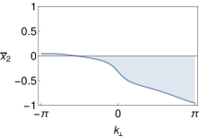
Figure 6: (color online) Position of the WCC for the first pair of Kramers degenerated band for a given set of the parameters, as the function of $k_{y}=k_{\perp}$. Depending on the band, we have $\Delta=\pm 1$, corresponding to a topological phase.

Another way to probe the topological nature of the system is to study the flow of the Wannier Charge Centers (WCC). King-Smith and Vanderbilt (1993); Yu et al. (2011) Indeed, as explained in the Appendix A, one may define the hybrid Wannier functions as per

$$|X,s,\alpha,k_{y}\rangle=\frac{1}{2\pi}\int_{-\pi}^{\pi}dk_{x}e^{-ik_{x}(X-\mathbf{\hat{X}})}|u^{s}_{\alpha,k_{x},k_{y}}\rangle.$$ (22)

The WCC are then defined as the expectation value $\bar{x}^{s}_{k_{y},\alpha}=\langle 0,s,\alpha,k_{y}|\hat{x}|0,s,\alpha,k_{y}\rangle$. The combination of time reversal and inversion symmetries requires that $\bar{x}^{I}_{k_{y},\alpha}+\bar{x}^{II}_{k_{y},\alpha}\in N$, meaning that the charge center of a pair of Kramers partner states lies at the unit cell center. However, the center of a single band may flow as $k_{y}$ varies, and this flow may characterize the topology of the system. To show this, we need to modify the definition of the topological invariant from the Eq. (9) as per

$$\Delta=P^{I}_{k_{y}=0}-P^{I}_{k_{y}=2\pi}\ mod\ 2.$$ (23)

Above, the two definitions were equivalent thanks to the choice of gauge in the Eq.(III.1) and the special choice of basis axes in the Appendix C, that yield

$$P^{I}_{k}=P^{II}_{-k}+N_{I},\ N_{I}\in\mathbb{N}$$ (24)

and

$$P^{I}_{k+G}=P^{I}_{k}+N_{G},\ N_{G}\in\mathbb{N}$$ (25)

Here, for convenience, we choose to treat $\mathbf{x}$ and $\mathbf{y}$ as basis vectors, Thus, the Eq.(24) is not valid anymore. Under this condition, the Eq.(23) is a better definition of the topological invariant than the Eq.(9), as it is directly related to the Chern number associated with the band corresponding to one of the two Kramers partners. The Eq.(23) transforms to

$$\Delta = \sum_{\alpha\in FB}(\bar{x}^{I}_{k_{y}=0,\alpha}-\bar{x}^{I}_{k_{y}=2\pi,\alpha})\ mod\ 2$$ (26)

$$= \sum_{\alpha\in FB}(\bar{x}^{I}_{k_{y}=-\pi,\alpha}-\bar{x}^{I}_{k_{y}=\pi,\alpha})\ mod\ 2.$$

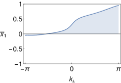
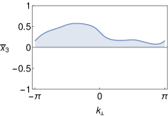
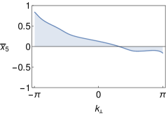
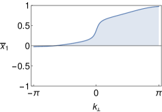
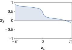
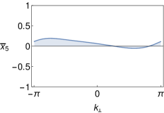
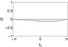
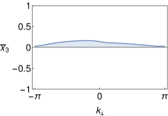
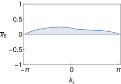
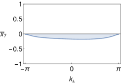
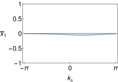
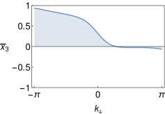
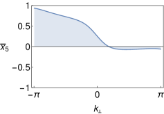
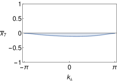
Figure 7: (color online) Position of the WCC as a function of $k_{\perp}$. The different columns correspond to a representative of the first, second, third and forth pair of bands in this order. The different lines correspond to $\Delta\mu=3$ (line 1 and 2) and $\Delta\mu=9$ (line 3 and 4), and $m=2$ (line 1 and 3) and $m=5$ (line 2 and 4).

Using the parallel transport method of the preceding subsection, we define the $|u^{s}_{\alpha,k_{x},k_{y}}\rangle$ that is smooth on a mesh in the BZ. Since $\bar{x}^{s}_{k_{y},\alpha}$is related to the Berry connection, we find

$$\bar{x}^{s}_{k_{y},\alpha} = i\frac{1}{2\pi}\int_{-\pi}^{\pi}dk_{x}\langle u^{s}_{\alpha,k_{x},k_{y}}|\nabla_{k_{x}}|u^{s}_{\alpha,k_{x},k_{y}}\rangle$$ (27)

$$= \frac{1}{2\pi}\sum_{j=1}^{\mathcal{N}}Im\langle u^{s}_{\alpha,j+1,k_{y}}|u^{s}_{\alpha,j,k_{y}}\rangle.$$

We observe that the topological invariant differs in sign when computed with one or the other Kramers partner (see the Fig. 6). However, as $\Delta$ is defined modulo 2, this sign has no physical meaning, and either of the two Kramers partners may be chosen.

The position of the WCC for one of the two Kramers partners of each pair of bands is plotted as a function of $k_{y}=k_{\perp}$ in the Fig. 7 for the same set of parameters as in the previous section. The results are once again in perfect agreement with the expected phase diagram of Fig. 3.

III.4 Explicit Construction of the Edge States

A defining property of $Z_{2}$ topological insulators is the existence of topologically-protected edge states. In time reversal invariant systems, a non-zero value of the topological invariant defined above corresponds to systems with an odd number of Kramers-degenerate pairs of edge states. Here, by explicitly constructing the edge states (adapting a method used for the BHZ Hamiltonian in [Konig et al., 2008]) we show that this bulk-edge correspondence holds in the AF case. It corroborates the importance of the time reversal polarization of the Eq.(17) also in the present case.

We consider a system defined on a semi-infinite plane and, hence, with a single edge. The direction of the cut will not be chosen arbitrarily, but in a way that respects the symmetries of the bulk, as shown in the Fig. 8. To be more explicit, a “good edge” would involve alternating A and B sites and is symmetric under $\Theta_{AF}=T\Theta$. By contrast, we will not consider here edges with only the A sites, as such an edge would manifest ferromagnetic order and would explicitly break the bulk symmetry $\Theta_{AF}$. Therefore, we choose the primitive lattice vectors to be $\mathbf{x}$ and $\mathbf{x}-\mathbf{y}$, and we choose a cut along $\mathbf{x}-\mathbf{y}$, at $\mathbf{x}=0$. This breaks the translation invariance along $\mathbf{x}$ while preserving it along $\mathbf{x}-\mathbf{y}$. Thus $k_{x-y}$ (denoted as $k_{\parallel}$) remains a good quantum number, but not the $k_{x}$.

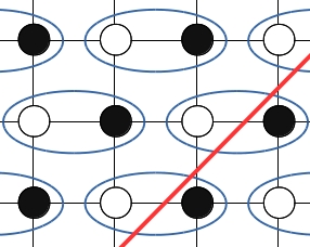
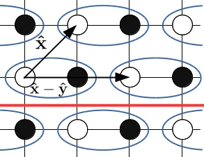
Figure 8: (color online) Examples of cuts (red lines) on the dimerised square lattice. (a) An example of an edge that does not respect the bulk symmetries (the $\Theta_{AF}$ symmetry is broken). (b) The edge considered in this article, and that respects the bulk symmetries. In this case, $k_{x-y}$ (noted $k_{\parallel}$) remains a good quantum number.

Hence, we write the Hamiltonian in terms of $k_{\parallel}$ and $-i\partial_{x}$ and look for the spatial extent of wave functions in the $x$ direction. In our special case, the Hamiltonian does not mix spin- up with spin-down, allowing us to consider only the $H^{\uparrow}_{k_{\parallel}}(-i\partial_{x})$ acting on the reduced Hilbert space made of spin-up states (the spin-down edge states can then be constructed using the $\Theta_{AF}$ operation). We now seek the solutions to

$$H^{\uparrow}_{k_{\parallel}}(-i\partial_{x})\Psi_{k_{\parallel}}(x)=E\Psi_{k_{\parallel}}(x)$$ (28)

with $E$ in the gap of the bulk spectrum. As we are looking for states exponentially localized at the edge, we use the ansatz $\Psi_{k_{\parallel}}(x)=e^{\lambda x}\Phi_{k_{\parallel}}$, with $\Phi$ independent of $x$, in Eq.(28). Cancelling the exponentials, we obtain the eigenvalue equation:

$$H^{\uparrow}_{k_{\parallel}}(-i\lambda)\Phi_{k_{\parallel}}=E\Phi_{k_{\parallel}}$$ (29)

that we will have to solve in $\lambda$ and $\Phi_{k_{\parallel}}$ simultaneously. Moreover, we will only keep solutions with $Re(\lambda)<0$, as we wish to obtain normalizable surface states. For a given value of $E$ and $k_{\parallel}$, we get several pairs of normalizable solutions $(\lambda^{i},\Phi^{i}_{k_{\parallel}})$ (generally, $i=1..4$). We could then build an edge state of the form:

$$\Psi_{edge}(x)=\sum_{i}C_{i}e^{\lambda^{i}x}\Phi^{i}_{k_{\parallel}}.$$ (30)

Given that the wave function must vanish at large negative $x$, we impose on the $\Psi_{edge}$ the boundary condition $\Psi_{edge}(0)=0$. This can only be done if the $\Phi^{i}_{k_{\parallel}}$ are linearly dependent, implying an existence condition for the edge state.

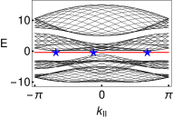
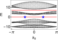
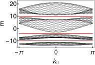
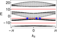
Figure 9: (color online) The projected dispersion relation on $k_{\parallel}$ is plotted in black for several values of the parameters. The red lines corresponds to the energy at which we looked for edge states using the technique described in III.4. The blue stars corresponds to the found spin-up edge states. An even number of spin-up edge states on a given line means that, at the given filling, the system is in the trivial phase, while an odd number of edge states corresponds to a topological insulator (a) $\Delta\mu=3$, $m=2$. (b) $\Delta\mu=3$, $m=5$. (c) $\Delta\mu=9$, $m=2$. (d) $\Delta\mu=9$, $m=2$. The results are in perfect agreement with the phase diagram of the Fig. 3. In (a) and (b), certain values of filling could not be studied because of semi-metallic character of the spectrum. As a result, the topological nature of the first pair of bands in (a) and (b) could not be verified with the present technique.

.

In practice, for an energy within the gap, we get 4 solutions for Eq. (29) and, as we work in the spin-up subspace, the $\Phi^{i}$ have four components. So, to analyse the linear dependence of the obtained solutions $\Phi^{i}$, we compute the determinant of the matrix formed by the four vectors, as a function of $k_{\parallel}$. We then extract the zeroes of this function. The number of zeros between $-\pi$ and $\pi$ corresponds to the number of spin-up edge states.

This number may vary depending on the parameter values. However, provided a gap present throughout the BZ, the parity of this number is directly related to the value of the topological invariant computed in the previous Section: $\Delta=0$ corresponds to an even number of spin-up edge states, while this number is odd when $\Delta=1$. This is true for the gap at half filing, which corresponds to the gap of the BHZ model, but also for the intermediate filling $1/4$ and $3/4$, as we can see, for some sets of parameters, in the Fig. 9.

For some values of the parameters, at 1/4 and 3/4 filling the band structure does not correspond to an insulator, as it has no forbidden energy band, as one may observe in the Figs. 9 (a,b): at such a filling the system is rather a semimetal (an optical insulator). Because of this, the edge state construction above cannot be applied directly: this method explicitly relies on the sought edge state having the energy where no bulk states exist. However, with the present Hamiltonian, we were unable to obtain both fully-insulating and topologically non-trivial behavior at 1/4 and 3/4 filling.

IV Application to non-centrosymmetric systems

So far, we considered the cases where numerical methods such as tracing either the Berry phase or the Wannier charge center trajectory could be tested against the product of parity eigenvalues at the TRIM, elegantly encapsulating the band topology. Now we would like to show that the former two methods allow one to study the band topology even when inversion is no longer a symmetry. In such a case parity is not a quantum number, and the $Z_{2}$ invariant cannot be related to the product of the parity eigenvalues at the TRIM.

To this end, we consider a perturbation to the Hamiltonian (II.2) that explicitly breaks the inversion symmetry, such as

$$H_{P}(\delta_{1},\delta_{2})=\delta_{1}\tau^{x}+2\delta_{2}(\sin(k_{x})+\sin(k_{y}))\sigma^{z}$$ (31)

where, as before $\tau$ matrices act in the orbital space and $\sigma$ matrices in the sublatice space. The first term corresponds to an on-site hybridization between the $p$ and $s$ orbitals, while the second term gives an inter-sublattice hoping. Each of the two breaks inversion symmetry and has the same qualitative effect as the combination we are considering here. We consider a combination of the two in order to illustrate a general case, where the inversion symmetry is lost, but the $\Theta_{AF}$ remains a symmetry.

The perturbation above lifts the double degeneracy, formerly protected by the combination of the $\Theta_{AF}$ and $\mathcal{P}_{AF}$, throughout the BZ – except for a line of points pinned at the TRIM. The Fig. 10 shows the degeneracy line between the third and fourth bands, i.e. the top two filled bands at half filling.

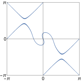
Figure 10: (color online) Degeneracy sub-manofild in the BZ for the third and fourth bands when the perturbation (31) is included. The values of the parameters here are $\delta_{1}=1.5$ and $\delta_{2}=0.5$

We concentrate on half-filling, and study the insulating gap between the (filled) bands 3 and 4 and the (empty) bands 5 and 6. For simplicity we fix all the parameters of the unperturbed Hamiltonian, as well as $\delta_{2}$. We then vary the $\delta_{1}$ to trigger the transition between the topological and topologically trivial phases. By choosing the same $t_{+}$ and $t_{-}$ as above, as well as $\alpha=1$, $\Delta\mu=9$, $m=5$ and $\delta_{2}=0.5$, we observe that the gap closes at $\delta^{*}_{1}\simeq 2.3$. For the sake of simplicity, we show here only the results obtained from the study of the WCC, but of course the study of the ”reconnection phase” gives the same result. The results are plotted in the Fig. 11 on the two sides of the transition. They clearly show that for $\delta_{1}<\delta^{*}_{1}$ the system is topologically non-trivial, while it becomes a trivial insulator for $\delta_{1}>\delta^{*}_{1}$.

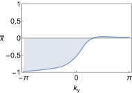
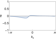
Figure 11: (color online) Analysis of the WCC cumulated on the two pairs of filled bands for the system with broken inversion symmetry. The values for $t_{+},t_{-}$ and $\alpha$ are chosen as before, and $\Delta\mu=9$, $m=5$ and $\delta_{2}=0.5$. The transition is obtained by varying $\delta_{1}$ and the critical point is found to be at $\delta^{*}_{1}\simeq 2.3$. The left side corresponds to $\delta_{1}=1.5$ and right to $\delta_{1}=3$.

Of course one can consider a wider variety of perturbation terms that break inversion symmetry. While for systems with genuine TR symmetry there is still the topological invariant (11) proposed by Fu and Kane, for system with an AF background no simple tool is available to predict topological phases. However, the extension of both the parallel transport and the WCC methods as presented in this article should allow a complete numerical identification of topological phases.

V conclusions, discussion and outlook

In the preceding chapters we presented two different methods to test the topology of an antiferromagnetic insulator. The first method is based on a parallel transport construction of Bloch eigenstates, while the second one traces the charge centers of mass of hybrid Wannier functions. The two methods were developed by adapting the techniques that have proven useful in diagnosing paramagnetic $Z_{2}$ topological insulators. Thus we provided a complete picture and phase diagram of the work initiated by Guo et al. in [Guo et al., 2011]. The methods we developed apply to any system with an anti-unitary momentum-inverting symmetry.

For centrosymmetric systems, defining a simple criterion of non-trivial topology was addressed in the Ref.[Fang et al., 2013]. This work proposed to consider the parity eigenvalues at the B-TRIM points only, while entirely disregarding their A-TRIM counterparts. In the case at hand, with the help of the methods developed above, we showed that this criterion does capture the topological phases correctly. However, for this criterion to hold, it is vital that there be no band inversion at the A-TRIM points. One may further argue that, in a more general model, any band inversion at one of the two A-TRIM points should occur at the other point as well, as long as there is a symmetry relating these two points. In the present case, the spatial ${\pi\over 2}$ rotation symmetry of the Hamiltonian ensures that the two A-TRIM points behave identically. As long as this is true, the criterion due to Fang et al. Fang et al. (2013) does capture a topological phase. However, if the two A-TRIM points are not symmetry-related, we see no reason that would protect the criterion due to Fang et al.

In the latter case, we expect the two methods developed above to prove useful for detecting topological phases. To further illustrate this point, we studied a generalization of our model to a non-centrosymmetric system, where we are no longer aware of a simple expression for a topological invariant, that would identify a topological phase. In spite of this, the methods developed above allowed us to pinpoint the transition between the trivial and topological phases.

VI Acknowledgments

It is our pleasure to acknowledge multiple discussions with Alexey A. Soluyanov, whose suggestions helped to greatly improve this work.

Appendix A Fu and Kane computation of the time reversal $Z_{2}$ topological invariant

In this Appendix, we give the details of the computation of the $Z_{2}$ topological invariant derived by Fu and Kane Fu and Kane (2006) in the time reversal symmetric case.

Here, we choose our primitive lattice vectors to be $X$ and $Y$. We define the reciprocal lattice vectors in a standard way, but we treat $k_{X}$ and $k_{Y}$ asymmetrically, and define the hybrid Bloch functions $|u^{s}_{\alpha,k_{X},k_{Y}}\rangle$ as

$$|\Psi^{s}_{\alpha,\mathbf{k}}\rangle=\frac{1}{\sqrt{N_{X}}}e^{ik_{X}\mathbf{\hat{X}}}|u^{s}_{\alpha,k_{X},k_{Y}}\rangle,$$ (32)

where $\mathbf{\hat{X}}$ is the position operator in the $\mathbf{X}$ direction, and $|\Psi^{s}_{\alpha,\mathbf{k}}\rangle$ is defined in Eq.(III.1) In the same spirit, we define the hybrid Wannier functions as:

$$|X,s,\alpha,k_{Y}\rangle=\frac{a}{2\pi}\int_{-\pi/a}^{\pi/a}dk_{X}e^{-ik_{X}(X-\mathbf{\hat{X}})}|u^{s}_{\alpha,k_{X},k_{Y}}\rangle$$ (33)

(in the same way, we define $|u_{n,k_{X},k_{Y}}\rangle$ and $|X,n,k_{Y}\rangle$ from the ${|\Psi_{n,\mathbf{k}}\rangle}$ that are used in Eq.(7).)

Following Fu and Kane, Fu and Kane (2006) we define the partial polarization $P^{s}_{k_{Y}}$, for a given value of $k_{Y}$ as:

$$P^{s}_{k_{Y}}=\sum_{\alpha}\langle 0,s,\alpha,k_{Y}|\mathbf{X}|0,s,\alpha,k_{Y}\rangle$$ (34)

for $s=\text{I}$ or II.

The total polarization is then equal to:

$$P^{\rho}_{k_{Y}}=P^{\text{I}}_{k_{Y}}+P^{\text{II}}_{k_{Y}},$$ (35)

while the time reversal polarization is defined as:

$$P^{\Theta}_{k_{Y}}=P^{\text{I}}_{k_{Y}}-P^{\text{II}}_{k_{Y}},$$ (36)

One may show that:

$$P^{s}_{k_{Y}}=\frac{a}{2\pi}\int_{-\pi/a}^{\pi/a}dk_{X}A^{s}_{k_{Y}}(k_{X})$$ (37)

with

$$A^{s}_{k_{Y}}(k_{X})=i\sum_{\alpha}\langle u^{s}_{\alpha,k_{X},k_{Y}}|\nabla_{k_{X}}|u^{s}_{\alpha,k_{X},k_{Y}}\rangle$$ (38)

After a computation described in the reference [Fu and Kane, 2006], for a gauge continuous over the BZ torus, we obtain:

$$P^{\Theta}_{\Gamma^{Y}}=\frac{a}{2\pi i}\bigg{[} \int_{0}^{\pi/a}dk_{X}\nabla_{k_{X}}\text{log\ det}[\mathit{w}(k_{X},\Gamma^{Y})]$$

$$-2\log\left(\frac{Pf[\mathit{w}(\pi/a,\Gamma^{Y}))]}{Pf[\mathit{w}(0,\Gamma^{Y}))}]\right)\bigg{]},$$ (39)

for $\Gamma^{Y}\in\{0,\pi/a\}$.

Using this expression, one can go from the definition in (9) to Eq.(11) in a straightforward way.

Appendix B Kramers degeneracy in the AF case

In this Appendix, we show that in the presence of commensurate staggered magnetization, and thus with broken time reversal symmetry, the inversion symmetry protects the Kramers degeneracy (see also the Refs. [Ramazashvili, 2008, 2009]). This is important for the definition of the eigenstates in the Eq.(III.1).

The system at hand possesses two important symmetries. The first one is associated with the operator

$$\Theta_{AF} =\sum_{\mathbf{k}}\Theta_{AF}(\mathbf{k})|-\mathbf{k}\rangle\langle\mathbf{k}|K$$

$$=\sum_{\mathbf{k}}ie^{i\frac{k_{x}-k_{y}}{2}}s^{y}\otimes(C_{-}\sigma^{x}-S_{-}\sigma^{y})|-\mathbf{k}\rangle\langle\mathbf{k}|K$$ (40)

which is anti-unitary and such that

$$\Theta_{AF}^{2} =-e^{i\Phi_{\mathbf{k}}}=-e^{-i2a\mathbf{k}\cdot\hat{\mathbf{X}}}.$$ (41)

The second symmetry is associated with

$$\mathcal{P}_{AF} =\sum_{\mathbf{k}}\mathcal{P}_{AF}(\mathbf{k})|-\mathbf{k}\rangle\langle\mathbf{k}|$$

$$=\sum_{\mathbf{k}}e^{i\frac{k_{x}-k_{y}}{2}}\tau^{z}\otimes(C_{-}Id+iS_{-}\sigma^{z})|-\mathbf{k}\rangle\langle\mathbf{k}|$$ (42)

which is unitary and squares to $1$.

The Kramers theorem arguments goes as follows: let $A$ be an anti-unitary operator that commutes with the Hamiltonian of the system and which square is $A^{2}=e^{i\theta}$ with $\theta\neq 0~{}mod~{}2\pi$. Let then $|\Psi\rangle$ be an eigenstate of $H$. Then $A|\Psi\rangle$ is also an eigenstate of $H$ with the same eigenvalue and

$$\langle\Psi|A|\Psi\rangle=0$$ (43)

The fact that $A|\Psi\rangle$ is also an eigenstate of $H$ is strait-forward for the commutativity of $A$ and $H$. The orthogonality (43) can be shown from the following equalities:

$$\langle{\Psi}|A\Psi\rangle=\langle{A\Psi}|AA\Psi\rangle^{*}=e^{-i\theta}\langle{A\Psi}|\Psi\rangle^{*}=e^{-i\theta}\langle{\Psi}|A\Psi\rangle$$ (44)

where the first equality follows from the fact that $A$ is anti-unitary, and the second from the property of $A^{2}$. Hence, if $\theta\neq 0~{}mod~{}2\pi$, $\langle\Psi|A|\Psi\rangle=0$.

In the case at hand, this result applies to the operator $\Theta_{AF}$ in the B-TRIM, and also to the operator $\Theta_{AF}\mathcal{P}_{AF}$ which is anti-unitary, commutes with the Hamiltonian, and squares to $-1$ in the entire BZ.

Then, the states $|\Psi_{n,\mathbf{k}}\rangle$ and $\Theta_{AF}\mathcal{P}_{AF}|\Psi_{n,\mathbf{k}}\rangle$ are degenerate and orthogonal, while carrying the same momentum label $\mathbf{k}$. Each band is thus doubly degenerate. Moreover, the states $\Theta_{AF}|\Psi_{n,\mathbf{k}}\rangle$ and $\mathcal{P}_{AF}|\Psi_{n,\mathbf{k}}\rangle$ are also degenerate and orthogonal, but carry the momentum label $\mathbf{-k}$.

So, we have Kramers pairs of states everywhere in the Brillouin Zone, that we can separate into $|\Psi^{I}_{\alpha,\mathbf{k}}\rangle$ and $|\Psi^{II}_{\alpha,\mathbf{k}}\rangle$. The problem is then to find a continuous definition of the $|\Psi^{I/II}\rangle$ on the BZ that respect Eq. (III.1). This is done in two steps.

The first step consists in finding a continuous definition of the $|\Psi^{I}_{\alpha,\mathbf{k}}\rangle$ over the BZ, that respects

$$\mathcal{P}_{AF}|\Psi^{I}_{\alpha,\mathbf{k}}\rangle=e^{i\phi(\mathbf{k})}|\Psi^{I}_{\alpha,\mathbf{-k}}\rangle$$ (45)

Then, we just need to construct $|\Psi^{II}_{\alpha,\mathbf{k}}\rangle=\Theta_{AF}\mathcal{P}_{AF}|\Psi^{I}_{\alpha,\mathbf{k}}\rangle$. The continuity of the $|\Psi^{II}\rangle$ states is a direct consequence of the continuity of the $|\Psi^{I}\rangle$, and Eq.(III.1) is a consequence of Eq.(45).

To properly define the $|\Psi^{I}_{\alpha,\mathbf{k}}\rangle$, we first choose a continuous definition of it for $k_{y}=0$ and $k_{x}\in\left[0,\pi\right]$ such that $\mathcal{P}_{AF}|\Psi^{I}_{\alpha,\mathbf{\Gamma}}\rangle$ is proportional to $|\Psi^{I}_{\alpha,\mathbf{\Gamma}}\rangle$ for $\mathbf{\Gamma}=(0,0)$ and $(\pi,0)$. Then, we construct the state at $k_{y}=0$ and $k_{x}\in\left]-\pi,0\right[$ as $|\Psi^{I}_{\alpha,\mathbf{k}}\rangle=\mathcal{P}_{AF}|\Psi^{I}_{\alpha,\mathbf{-k}}\rangle$. This definition may be discontinuous at $k_{x}=0$ and $k_{x}=\pi$, but we have:

$$\lim_{k_{x}\rightarrow 0^{+}}|\Psi^{I}_{\alpha,-k_{x},k_{y}=0}\rangle =\lim_{k_{x}\rightarrow 0^{+}}\mathcal{P}_{AF}|\Psi^{I}_{\alpha,k_{x},k_{y}=0}\rangle$$

$$=\mathcal{P}_{AF}|\Psi^{I}_{\alpha,k_{x}=0,k_{y}=0}\rangle$$

$$=e^{i\phi(0)}|\Psi^{I}_{\alpha,k_{x}=0,k_{y}=0}\rangle$$ (46)

and a similar phase appears at $k_{x}=\pi$. To get rid of this phase, we multiply all states at $k_{y}=0$ and $k_{x}\in\left]-\pi,0\right[$ by a continuous phase $e^{-i\phi(k_{x})}$ such that $\lim_{k_{x}\rightarrow 0^{-}}e^{i\phi(k_{x})}=e^{i\phi(0)}$ and $\lim_{k_{x}\rightarrow-\pi}e^{i\phi(k_{x})}=e^{i\phi(\pi)}$. We end up with a definition of $|\Psi^{I}_{\alpha,\mathbf{k}}\rangle$ that is continuous along the circle $k_{y}=0$ and that respects Eq.(45). This set of states can now be continuously extended to the entire upper half of the Brillouin zone ($k_{y}\in\left]0,\pi\right]$) in a way described in [Soluyanov and Vanderbilt, 2012]. We apply $\mathcal{P}_{AF}$ to construct the states in the lower half of the Brillouin zone. Once again, we may have a discontinuity while crossing the line $k_{y}=0$, but we recover continuity by multiplying all the states with $k_{y}<0$ by the phase $e^{-i\phi{|k_{x}|}}$.

As was said before, we can now apply $\Theta_{AF}\mathcal{P}_{AF}$ to construct the $|\Psi^{II}_{\alpha,\mathbf{k}}\rangle$ states, and get a continuous definition over the cylindrical BZ with edges $k_{y}=\pi$ and $k_{y}=-\pi$, that respects Eq. (III.1).

Appendix C Computation of the $Z_{2}$ invariant in the AF case

In this Appendix, we define the hybrid Bloch states and the hybrid Wannier functions as in Appendix A, the goal being once again to compute the time reversal polarization, but in the case of broken time reversal symmetry. In Appendix A, we showed how to get an expression of the $Z_{2}$ topological invariant in terms of the determinant and the pfaffian of the sewing matrix at the four TRIM (Eq.(11)). In order to define the Pfaffian, we needed the sewing matrix to be anti-symmetric at the four TRIM. However, in the case of the added staggered magnetization, the sewing matrix defined with $\Theta_{AF}$ is symmetric at the A-TRIM (TRIM where $\Theta_{AF}^{2}=1$). This is why, in the AF case, we do not get an expression (16) for the $Z_{2}$ invariant only in terms of the sewing matrix, but also in terms of the phase $\chi$.

As in the time reversal symmetric case, we consider two primitive lattice vectors $\mathbf{a}$ and $\mathbf{b}$. We make the Wannier transformation along $\mathbf{a}$, while keeping plane waves along $\mathbf{b}$. We now wish to compute $P^{\Theta_{AF}}_{\Gamma_{b}}=P^{\text{I}}_{\Gamma_{b}}-P^{\text{II}}_{\Gamma_{b}}$.

We first concentrate on $P^{\text{I}}_{\Gamma_{b}}$. Equation (37) for $s=\text{I}$ may be rewritten as:

$$P^{\text{I}}_{\Gamma_{b}} = \frac{1}{2\pi}\int_{0}^{\pi}dk_{a}[A^{\text{I}}_{\Gamma_{b}}(k_{a})+A^{\text{I}}_{\Gamma_{b}}(-k_{a})]$$ (47)

Moreover, using Eqs.(III.1) and (38) and the antiunitarity of $\Theta_{AF}$, one may show that:

$$A^{\text{I}}_{-k_{b}}(-k_{a}) = A^{\text{II}}_{k_{b}}(k_{a})+\sum_{\alpha}\nabla_{k_{a}}(\chi_{\alpha,k_{a},k_{b}}+\frac{1}{2}\Phi_{k_{a},k_{b}})$$

$$+ i\sum_{\alpha}\langle u^{\text{ II}}_{\alpha,k_{a},k_{b}}|(\nabla_{k_{a}}\hat{\Theta}_{AF}(\mathbf{k}))\hat{\Theta}_{AF}(\mathbf{k})^{\dagger}|u^{\text{ II}}_{\alpha,k_{a},k_{b}}\rangle$$

Because of the derivatives of $\Theta_{AF}$ and $\Phi$, this expression may seem not very useful. But $\Theta_{AF}$ and $\Phi$ both depends only on $k_{x}-k_{y}$. So, if we choose $k_{a}=k_{x}$ and $k_{b}=k_{x}-k_{y}$, the derivative term disappear and we get:

$$A^{\text{I}}_{-k_{b}}(-k_{a}) = A^{\text{II}}_{k_{b}}(k_{a})+\sum_{\alpha}\nabla_{k_{a}}\chi_{\alpha,k_{a},k_{b}}$$ (49)

And so,

$$P^{\text{I}}_{\Gamma_{b}} = \frac{1}{2\pi}\int_{0}^{\pi}dk_{a}(A^{I}_{-\Gamma_{b}}(k_{a})+A^{II}_{\Gamma_{b}}(k_{a}))$$ (50)

$$+ \frac{1}{2\pi}\sum_{\alpha}(\chi_{\alpha,\pi,-\Gamma_{b}}-\chi_{\alpha,0,-\Gamma_{b}})$$

Finally, using $P^{\Theta_{AF}}_{\Gamma_{b}}=2P^{\text{I}}_{\Gamma_{b}}-P^{\rho}_{\Gamma_{b}}$, and folowing Fu and Kane, Fu and Kane (2006) this can be rewritten in a continuous gauge as:

$$P^{\Theta_{AF}}_{\Gamma_{b}} = \frac{1}{2\pi i}\int_{0}^{\pi}dk_{a}\nabla_{k_{a}}\text{log\ det}[\tilde{\mathit{w}}_{\Gamma_{b}}(k_{a})]$$ (51)

$$+\frac{1}{\pi}\sum_{\alpha}(\chi_{\alpha,0,\Gamma_{b}}+\chi_{\alpha,\pi,\Gamma_{b}})$$

where $\tilde{\mathit{w}}$ is the sewing matrix defined by:

$$\tilde{\mathit{w}}_{k_{b}}(k_{a})_{mn}=\langle\Psi_{m,\mathbf{-k}}|\Theta_{AF}|\Psi_{n,\mathbf{k}}\rangle.$$ (52)

References

- Hasan and Kane (2010) M. Z. Hasan and C. L. Kane, Rev. Mod. Phys. 82, 3045 (2010), URL http://link.aps.org/doi/10.1103/RevModPhys.82.3045.
- Qi and Zhang (2011) X.-L. Qi and S.-C. Zhang, Rev. Mod. Phys. 83, 1057 (2011), URL http://link.aps.org/doi/10.1103/RevModPhys.83.1057.
- Kane and Mele (2005a) C. L. Kane and E. J. Mele, Phys. Rev. Lett. 95, 226801 (2005a), URL http://link.aps.org/doi/10.1103/PhysRevLett.95.226801.
- Kane and Mele (2005b) C. L. Kane and E. J. Mele, Phys. Rev. Lett. 95, 146802 (2005b), URL http://link.aps.org/doi/10.1103/PhysRevLett.95.146802.
- Xu and Moore (2006) C. Xu and J. E. Moore, Phys. Rev. B 73, 045322 (2006), URL http://link.aps.org/doi/10.1103/PhysRevB.73.045322.
- Wu et al. (2006) C. Wu, B. A. Bernevig, and S.-C. Zhang, Phys. Rev. Lett. 96, 106401 (2006), URL http://link.aps.org/doi/10.1103/PhysRevLett.96.106401.
- Bernevig et al. (2006) B. A. Bernevig, T. L. Hughes, and S.-C. Zhang, Science 314, 1757 (2006), URL http://www.sciencemag.org/content/314/5806/1757.abstract.
- Mong et al. (2010) R. S. K. Mong, A. M. Essin, and J. E. Moore, Phys. Rev. B 81, 245209 (2010), URL http://link.aps.org/doi/10.1103/PhysRevB.81.245209.
- Liu (2013) C.-X. Liu, ArXiv e-prints (2013), eprint 1304.6455.
- Zhang and Liu (2015) R.-X. Zhang and C.-X. Liu, Phys. Rev. B 91, 115317 (2015), URL http://link.aps.org/doi/10.1103/PhysRevB.91.115317.
- Liu et al. (2014) C.-X. Liu, R.-X. Zhang, and B. K. VanLeeuwen, Phys. Rev. B 90, 085304 (2014), URL http://link.aps.org/doi/10.1103/PhysRevB.90.085304.
- Fang and Fu (2015) C. Fang and L. Fu, Phys. Rev. B 91, 161105 (2015), URL http://link.aps.org/doi/10.1103/PhysRevB.91.161105.
- Fang et al. (2013) C. Fang, M. J. Gilbert, and B. A. Bernevig, Phys. Rev. B 88, 085406 (2013), URL http://link.aps.org/doi/10.1103/PhysRevB.88.085406.
- Fu (2011) L. Fu, Phys. Rev. Lett. 106, 106802 (2011), URL http://link.aps.org/doi/10.1103/PhysRevLett.106.106802.
- Kargarian and Fiete (2013) M. Kargarian and G. A. Fiete, Phys. Rev. Lett. 110, 156403 (2013), URL http://link.aps.org/doi/10.1103/PhysRevLett.110.156403.
- Liu et al. (2013) J. Liu, W. Duan, and L. Fu, Phys. Rev. B 88, 241303 (2013), URL http://link.aps.org/doi/10.1103/PhysRevB.88.241303.
- Serbyn and Fu (2014) M. Serbyn and L. Fu, Phys. Rev. B 90, 035402 (2014), URL http://link.aps.org/doi/10.1103/PhysRevB.90.035402.
- Jadaun et al. (2013) P. Jadaun, D. Xiao, Q. Niu, and S. K. Banerjee, Phys. Rev. B 88, 085110 (2013), URL http://link.aps.org/doi/10.1103/PhysRevB.88.085110.
- Fu and Kane (2007) L. Fu and C. L. Kane, Phys. Rev. B 76, 045302 (2007), URL http://link.aps.org/doi/10.1103/PhysRevB.76.045302.
- Soluyanov and Vanderbilt (2012) A. A. Soluyanov and D. Vanderbilt, Phys. Rev. B 85, 115415 (2012), URL http://link.aps.org/doi/10.1103/PhysRevB.85.115415.
- King-Smith and Vanderbilt (1993) R. D. King-Smith and D. Vanderbilt, Phys. Rev. B 47, 1651 (1993), URL http://link.aps.org/doi/10.1103/PhysRevB.47.1651.
- Yu et al. (2011) R. Yu, X. L. Qi, A. Bernevig, Z. Fang, and X. Dai, Phys. Rev. B 84, 075119 (2011), URL http://link.aps.org/doi/10.1103/PhysRevB.84.075119.
- Kulikov and Tugushev (1984) N. I. Kulikov and V. V. Tugushev, Physics-Uspekhi 27, 954 (1984), URL http://ufn.ru/en/articles/1984/12/c/.
- Ramazashvili (2008) R. Ramazashvili, Phys. Rev. Lett. 101, 137202 (2008), URL http://link.aps.org/doi/10.1103/PhysRevLett.101.137202.
- Ramazashvili (2009) R. Ramazashvili, Phys. Rev. B 79, 184432 (2009), URL http://link.aps.org/doi/10.1103/PhysRevB.79.184432.
- Guo et al. (2011) H. Guo, S. Feng, and S.-Q. Shen, Phys. Rev. B 83, 045114 (2011), URL http://link.aps.org/doi/10.1103/PhysRevB.83.045114.
- Fruchart et al. (2014) M. Fruchart, D. Carpentier, and K. Gawedzki, EPL (Europhysics Letters) 106, 60002 (2014), URL http://stacks.iop.org/0295-5075/106/i=6/a=60002.
- Fu and Kane (2006) L. Fu and C. L. Kane, Phys. Rev. B 74, 195312 (2006), URL http://link.aps.org/doi/10.1103/PhysRevB.74.195312.
- Konig et al. (2008) M. Konig, H. Buhmann, L. W. Molenkamp, T. Hughes, C.-X. Liu, X.-L. Qi, and S.-C. Zhang, Journal of the Physical Society of Japan 77, 031007 (2008), URL http://dx.doi.org/10.1143/JPSJ.77.031007.