Record breaking bursts during the compressive failure of porous materials

Abstract

An accurate understanding of the interplay between random and deterministic processes in generating extreme events is of critical importance in many fields, from forecasting extreme meteorological events to the catastrophic failure of materials and in the Earth. Here we investigate the statistics of record-breaking events in the time series of crackling noise generated by local rupture events during the compressive failure of porous materials. The events are generated by computer simulations of the uni-axial compression of cylindrical samples in a discrete element model of sedimentary rocks that closely resemble those of real experiments. The number of records grows initially as a decelerating power law of the number of events, followed by an acceleration immediately prior to failure. The distribution of the size and lifetime of records are power-laws with relatively low exponents. We demonstrate the existence of a characteristic record rank $k^{*}$ which separates the two regimes of the time evolution. Up to this rank deceleration occurs due to the effect of random disorder. Record breaking then accelerates towards macroscopic failure, when physical interactions leading to spatial and temporal correlations dominate the location and timing of local ruptures. Scaling analysis revealed that the size distribution of records of different ranks has a universal form independent of the record rank. Sub-sequences of bursts between consecutive records are characterized by a power law size distribution with an exponent which decreases as failure is approached. High rank records are preceded by bursts of increasing size and waiting time between consecutive events and they are followed by a relaxation process. As a reference, surrogate time series are generated by reshuffling the crackling bursts. The record statistics of the uncorrelated surrogates agrees very well with the corresponding predictions of independent identically distributed random variables, which confirms that the temporal and spatial correlation of cracking bursts are responsible for the observed unique behaviour. In principle the results could be used to improve forecasting of catastrophic failure events, if they can be observed reliably in real time.

I Introduction

The compressive failure of heterogeneous materials proceeds in bursts of cracking events. Measuring the generated acoustic emissions is the primary source of information about the time evolution of the fracture process Sammonds et al. (1992); Ojala et al. (2004); Mair et al. (2000); Henderson et al. (1992); Rosti et al. (2009); Nataf et al. (2014); Castillo-Villa et al. (2013). The statistical analysis of the stochastic time series of crackling bursts in field data, laboratory experiments, and in computer simulations has provided a useful insight into the accumulation of damage and into the approach of the system to macroscopic failure. The ultimate challenge of the field is to find statistical signatures which could be exploited to forecast the impending catastrophic failure Main (1996). For this purpose the analysis of synthetic time series of simulated fracture processes is indispensible since they allow a range of variables to be controlled and investigated independently, and allow representative sampling of underlying trends and statistical variability over a large number of trials Alava et al. (2006); Hidalgo et al. (2009).

Recently, we have introduced a discrete element model of porous sedimentary rocks which captures the essential ingredients of the materials’ micro-structure and of the dynamics of breaking Kun et al. (2013, 2014). The model was used to investigate the compressive failure of cylindrical samples under strain controlled conditions. During the failure process we identify cracking bursts as correlated trails of breaking beams which are generated due to the gradual stress redistribution in the sample following local failure events Kun et al. (2013, 2014).

In the present paper we investigate the internal structure of the time series of breaking bursts by analyzing the statistical features of record breaking (RB) events. Records are bursts which have a size greater than any previous events of the series. Recently, the record statistics of stochastic time series has attracted great attention due to its relevance for climate and earthquake research Wergen and Krug (2010); Davidsen et al. (2006, 2008); Yoder et al. (2010). Interesting analytic results have been obtained for the RB statistics of the sequences of independent identically distributed (IID) random variables for a randomly-sampled stationary process Wergen (2013); Shcherbakov et al. (2013); Yoder et al. (2010). In physics the statistics of records has been applied to understand correlated processes emerging in various types of random walks Majumdar and Ziff (2008); Majumdar et al. (2012); Godreche et al. (2014), superconductors Oliveira et al. (2005), domain wall dynamics in spin glasses Jensen (2006), and in chaotic processes Srivastava and Lakshminarayan (2015). The record statistics of the bursting activity has also been studied recently in models exhibiting self organized criticality (SOC) Shcherbakov et al. (2013) and in a mean field model of fracture Danku and Kun (2014). For earthquakes record statistics were recently applied to reveal spatiotemporal clustering of seismicity either by focusing on the inter event times Yoder et al. (2010) or using both the spatial and temporal distance of events Davidsen et al. (2006, 2008). In our realistic discrete element model of compressive failure we analyze both the aggregated statistics of records and the evolution of record breaking as the sample approaches macroscopic failure. As a null hypothesis we compare our results to the IID findings and to the record statistics of a surrogate data set where correlations are destroyed by randomly reshuffling the breaking bursts of fracture simulations. This comparison makes it possible to reveal interesting trends and correlations in the spatial and temporal signature of the crackling noise. We show significant departures associated with non-stationary processes associated with increased strain, and reveal new signatures of impending catastrophic failure in the time series associated with record-breaking events.

II Record breaking events

We study the statistics of records in a synthetic time series of breaking bursts generated by a discrete element model (DEM). The model has been developed recently to investigate the emergence of crackling noise during the compressive failure of cylindrical samples of porous rocks Kun et al. (2013, 2014). The rock sample was reconstructed on the computer by sedimenting spherical particles with a realistic size distribution. The particles are coupled by cohesive contacts represented by beam elements which break when they are stressed beyond a limit. Strain controlled uniaxial compression was realized by clamping a few particle layers at the bottom and at the top of the sample. The bottom was fixed, while the top layers were moved at a constant speed along the cylinder axis. The loading process was stopped when the force acting on the top layer dropped down to zero. Due to the subsequent load redistribution following failure events beams break in cascades analogous to crackling avalanches in real materials. In Refs. Kun et al. (2013, 2014) we investigated the dynamics of emergence and statistics of such crackling bursts during the strain controlled uniaxial compression of cylindrical samples composed of 20000 particles. The modeling approach proved to be successful in reproducing several important observed features of crackling noise in porous materials Baró et al. (2013); Nataf et al. (2014); Castillo-Villa et al. (2013); Sammonds et al. (1992); Ojala et al. (2004); Mair et al. (2000).

Figure 1 demonstrates the breaking sequence of a single simulation of a system of 20000 particles where 1832 bursts are obtained up to macroscopic failure in comparison with data from a real experiment Lennartz-Sassinek et al. (2014). In the example the breaking process starts at the deformation $\varepsilon\approx 0.0019$

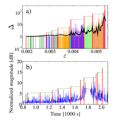
Figure 1: (Color online) $(a)$ Sequence of breaking bursts in a single simulation, i.e. the size of events $\Delta$ as a function of the strain $\varepsilon$ where they occurred. Record events are highlighted by red bars, while sub-sequences between records have randomly assigned colors. The bold continuous line represents the moving average of burst sizes using 30 consecutive events. For clarity, a relatively small system of 20000 particles was considered, where $n_{max}=1832$ bursts occurred with 10 records. $(b)$ Record events in a time series of a real fracture experiment performed under conditions similar to the simulations Lennartz-Sassinek et al. (2014).

where initially small bursts occur with size $\Delta=1$. As loading proceeds larger and larger bursts are triggered so that the average burst size steadily increases towards failure although $\Delta$ has strong fluctuations due to the disordered micro-structure of the material.

Records of the event series are bursts which have a size $\Delta$ greater than any previous event. RB events are identified by their rank $k=1,2,\ldots$ which occurred as the $n_{k}$th event of the complete time series with size $\Delta_{r}^{k}$. By definition the first event $n=1$ of the series is a record so that $n_{1}=1$ holds. Figure 1 illustrates that RB bursts form a monotonically increasing sub-sequence and divide the time series into segments of varying number of smaller size events. The presence of RB events has a complex effect on the local structure of the time series in Fig. 1: the moving average of the event size tends to peak at the time of record-breaking events, with a precursory increase in the average burst size, followed by a decrease or relaxation after the record-breaking event. This pattern is more pronounced close to failure.

To characterize how record breaking evolves during the loading process, we also consider the size increments $\delta_{r}^{k}$ and the waiting times $m_{k}$ between consecutive records defined as

$$\delta_{r}^{k} = \Delta_{r}^{k+1}-\Delta_{r}^{k},$$ (1)

$$m_{k} = n_{k+1}-n_{k},$$ (2)

respectively. After analyzing the overall statistics of record quantities, we focus on the evolution of the sequence of RB events as the system approaches failure. Finally, we study how records influence the structure of the time series of crackling events.

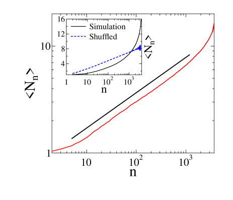
Figure 2: (Color online) Average number of records $\left<N_{n}\right>$ occurred until the $n$th burst as a function of $n$ on a double logarithmic plot. Power law behavior is obtained over a broad range of $n$. The straight line represents a power law of exponent $0.33$. The inset presents the same quantity $\left<N_{n}\right>$ on a semi-logarithmic plot. For comparison the shuffled data set is also included where a logarithmic dependence is found.

Based on the statistics of extremes it has been shown for sequences of independent identically distributed random variables (IID) that the statistics of record breakings has universal features, i.e. several statistical measures of IID records do not depend on the underlying probability distribution of individual events Wergen (2013). The increasing average event size and decreasing waiting time between consecutive events in Fig. 1 demonstrate that the time series of crackling bursts accompanying compressive failure is highly non-stationary. Comparing the results of our analysis to the corresponding results of IIDs enables us to quantify the competing role of the structural disorder of the material and of the stress enhancements around failed regions, which favorably lead to a stationary sequence of uncorrelated events Main (2000); Mair et al. (2000); Heap et al. (2011); Main et al. (2000) and to an accelerating sequence with spatial and temporal correlations Kun et al. (2014, 2013); Mair et al. (2000); Heap et al. (2011); Main et al. (2000), respectively. Additionally, we generate a surrogate data set by reshuffling the events of the simulated time series to destroy correlations. For each fracture simulation the indices $n$ of events are permutated and then the same analysis was performed as for the original data. When it is applicable, the results of the original data, its suffled counterpart, and the IID predictions are presented together in the figures. For the data evaluations the statistical toolbox of MATLAB was extensively used MATLAB (2010) where a non-linear least square method was used for curve fitting.

In the present study careful parallelization of the computer code allowed us to substantially increase the system size. Here simulations were performed with a particle number fluctuating around $10^{5}$ such that on the average the diameter of the cylinder is spanned by about 50 particles while the height to diameter aspect ratio of the sample is 2.3 Kun et al. (2013, 2014). For an average particle size of 200 microns (typical reservoir sandstone) the sample diameter would correspond to 1cm which gets near to the typical small core lab sample diameter of 2.5 cm. In a single simulation we identified $n_{max}=3500-4000$ bursts of beam breakings. Averages of all quantities are calculated over 550 simulations.

III Number of records

Since records are major bursts of the breaking process which have a dominating contribution to the accumulating damage, it is of high interest how the number of records $N_{n}$ increases with the number of events $n$. For IIDs it has been shown that the average number of records $\left<N_{n}\right>$ that occurred until the event number $n$ has been reached grows logarithmically with $n$

$$\left<N_{n}\right>\sim\kappa+\ln n+\mathcal{O}(1/n),\qquad\mbox{for}\qquad n\to+\infty,$$ (3)

independently of the specific form of the probability density of the random variables Wergen (2013). Here $\kappa$ denotes the Euler-Mascheroni constant $\kappa\approx 0.577215665$ Wergen (2013); Shcherbakov et al. (2013). For crackling noise accompanying the quasi-static loading of heterogeneous materials deviations from this behavior can be expected: due to the increase of the externally imposed strain the failure process accelerates so that larger bursts are triggered which follow each other after shorter waiting times Kun et al. (2013, 2014). The complex redistribution of stress inside the damaged sample gives rise to the emergence of temporal and spatial correlations of bursts of the sequence. As a consequence, the number of records increases as a power law of the event number

$$\left<N_{n}\right>\sim n^{\alpha},$$ (4)

over a broad range of $n$ (see Figure 2). The value of the exponent was obtained numerically $\alpha=0.33\pm 0.03$. This value of $\alpha$ indicates that the number of record-breaking events also increases at a decelerating rate, albeit with a different form to that of Eq. (3). Deviations from the power law can be observed at the very beginning of the loading process and in the close vicinity of macroscopic failure. The up-turn of the $\left<N_{n}\right>$ curve in Fig. 2 for the highest event indices $n$ shows that as failure is approached the rate of record-breaking accelerates (the local slope increases). This acceleration generally occurs when the record number $N_{n}$ exceeds 7. The inset of Fig. 2 presents $\left<N_{n}\right>$ on a semi-logarithmic plot. Strong deviation can be observed from a straight line which confirms that the functional form is not logarithmic.

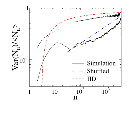
Figure 3: (Color online) Standard deviation of the number of records $Var(N_{n})$ occurred until the $n$th burst divided by the average record number $\left<N_{n}\right>$ on a double logarithmic plot. The red (dashed) and the blue (dashed-dotted) lines represent the corresponding result of the shuffled data set and a power law of exponent 1/3, respectively.

The corresponding curve of the shuffled data is also presented in the inset, which has a perfect agreement with the analytical IID result Eq. (3). From Figure 2$(inset)$ the null hypothesis of sampling from a parent distribution can be rejected. Instead we have a decelerating transient response of a power-law form.

To characterize the sample-to-sample variation of the number of records $N_{n}$ we calculated the standard deviation

$$Var(N_{n})=\left<(N_{n}-\left<N_{n}\right>)^{2}\right>.$$ (5)

For IIDs the analytic solution gives again an asymptotic logarithmic increase with $n$ as Wergen (2013); Shcherbakov et al. (2013)

$$Var(N_{n})=\kappa+\ln n-\frac{\pi^{2}}{6}+\mathcal{O}(1/n),\quad\mbox{for}\quad n\to+\infty,$$ (6)

so that the relative variance $Var(N_{n})/\left<N_{n}\right>$ monotonically increases and tends to 1 for sufficiently large $n$. Figure 3 presents that the very beginning of our fracture process, up to about $n=10$ bursts, is consistent with the IID behaviour. However, after a short intermediate decreasing regime the curve sets to a faster increase which has a nearly power law functional form. In Fig. 3 a power law of the same exponent as for the average record number in Fig. 2 is drawn to guide the eye. The result of the shuffled data is again consistent with the IID solution.

The probability distribution of the number of records $p(N_{n})$ that occurred up to a fixed number $n$ of events has been found to have a Gaussian functional form for IIDs in the limit of large $n$ values Wergen (2013); Shcherbakov et al. (2013). Figure 4 shows that in our fracture process the distribution $p(N_{n}^{tot})$ of the total number of records $N_{n}^{tot}$ that occurred up to failure is similar to a Gaussian with an average $\left<N_{n}^{tot}\right>=18.1$ and standard deviation $Var(N_{n}^{tot})=3.1$.

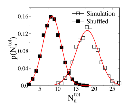
Figure 4: (Color online) Probability distribution of the total number of records $p(N_{n}^{tot})$ that occurred up to failure for the original and surrogate data sets. The continuous lines represent the Gaussian distributions obtained with the mean and standard deviation calculated directly from the data.

The highest and lowest number of records we identified in single simulations were 10 and 26, respectively, with the most probable value 18. In the shuffled event series large size events can occur anywhere which results in a significantly lower number of records $\left<N_{n}^{tot}\right>=8.4$ with a standard deviation $Var(N_{n}^{tot})=2.5$. The continuous lines in Fig. 4 represent Gaussian distributions obtained by inserting the corresponding values of $\left<N_{n}^{tot}\right>$ and $Var(N_{n}^{tot})$ for the two data sets. Both for the simulated and surrogate data reasonable agreement is obtained with the Gaussian distribution.

IV Distribution of record sizes

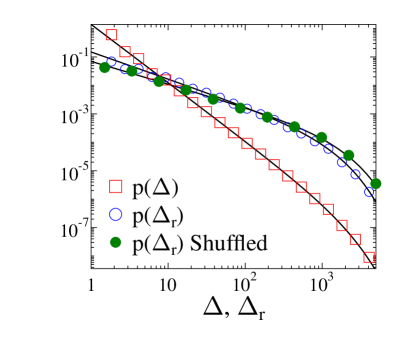
Figure 5: (Color online) Probability distribution $p(\Delta)$ of the burst size $\Delta$ considering all events up to failure. The size distribution of records $p(\Delta_{r})$ is presented both for the original and surrogate data sets. In all cases the bold lines represent best fits with Eq. (7) obtained with the parameter values: $\xi=2.15$, $c=1.0$ and $\Delta^{*}=1810$ for $p(\Delta)$, $\xi_{r}=1.0$, $c_{r}=0.9$ and $\Delta_{r}^{*}=1052$ for $p(\Delta_{r})$, and $\xi_{r}^{s}=0.8$, $c_{s}=0.9$ and $\Delta_{s}^{*}=1270$ for for shuffled series.

Recently, we have shown that the size distribution of bursts $p(\Delta)$ accumulating all events up to failure during the compression process has a power law functional form followed by an exponential cutoff

$$p(\Delta)\sim\Delta^{-\xi}\exp{\left[-(\Delta/\Delta^{*})^{c}\right]}.$$ (7)

In Refs. Kun et al. (2013, 2014) the exponent $\xi$ was obtained numerically as $\xi=2.15$ for samples comprising 20000 particles. In the present study $10^{5}$ particles are used which gives the same exponent for $p(\Delta)$, however, with a broader power law regime in Fig. 5. Thus there is no evidence of scale-dependence in the power-lay exponent, only an increase in the characteristic size $\Delta^{*}$, and hence in the bandwidth of the power-law behaviour.

Records form a subset of events of the complete series containing solely the largest bursts that occurred up to a given event index. Figure 5 shows that the distribution of the size of records $p(\Delta_{r})$ has the same functional form Eq. (7) as the size distribution of all events $p(\Delta)$, however, the exponent $\xi_{r}$ of the power law regime is significantly lower $\xi_{r}=1.0\pm 0.05$ than for the complete distribution $\xi$. Selecting RB events implies a resampling of the ensemble of bursts, where the distribution of the record size is governed by the statistics of extremes. The difference in slope is likely caused by the inherent sample bias in choosing record breaking events either $(a)$ because this preferentially filters out smaller events and/or $(b)$ larger events may be associated with a greater degree of local stress concentration (stress intensity), known to be associated with a flatter slope Sammonds et al. (1992). In the shuffled event series large size events can occur earlier than during the original fracture process so that small size events have a lower chance to become a record. As a consequence, the size distribution of shuffled records has the same functional form, however, with a lower exponent $\xi_{r}^{s}=0.8\pm 0.07$, which indicates the lower fraction of small records.

V Approach to failure through breaking of records

The integrated statistics of records presented above gives an overall description of the subset of RB events of the crackling time series. It is a question of fundamental interest how the system approaches failure through a sequence of record breaking events. To obtain a quantitative understanding we calculated averages of characteristic quantities of records as a function of the record rank $k$. Figure 6$(a)$ shows that as the system evolves the average size of records $\left<\Delta_{r}^{k}\right>$ rapidly increases with $k$. The size increments $\left<\delta_{r}^{k}\right>$ exhibit qualitatively the same behavior, i.e. during the entire failure process records get broken with an increasing sequence of increments. The shuffled data set has the same qualitative tendencies with the difference that low rank records reach higher sizes than in the original data.

Figure 6: (Color online) Average value of the characteristic quantities of records as a function of the record rank $k$: size and increment $(a)$, relative increment $(b)$, waiting time $(c)$, and strain of records normalized by the critical strain of failure $(d)$. The Grey stripe highlights the strain range between the records of rank $k=7$ and $k=8$. In $(a),(b),(c)$ the open and filled symbols represent the original and the surrogate data sets, respectively.

For a stationary sequence of IIDs the extreme value statistics leads to a monotonous decrease of average relative increments between consecutive records Miller and Ben-Naim (2013). This is what we find for the early part of our time series, when the timing and size of events is dominated by the random structural disorder. However, for the later RB events we find the opposite, i.e. an accelerating trend, most likely associated with processes dominated by the dynamics, such as stress relaxation and redistribution, and localization of events on to the eventual failure plane. This change from decelaration to acceleration is illustrated in Figure 6$(b)$ where the average value of the relative increment $\left<\delta_{r}^{k}/\Delta_{r}^{k}\right>$ is presented. Initially the RB process slows down, i.e. up to a characteristic record rank $k^{*}=7-8$ the relative increment $\left<\delta_{r}^{k}/\Delta_{r}^{k}\right>$ decreases, while for higher ranks $k>k^{*}$ the onset of accelerating fracture is marked by the increase of $\left<\delta_{r}^{k}/\Delta_{r}^{k}\right>$. The result is also supported by the behaviour of the surrogate data where correlation are destroyed: the relative increment monotonically decreases without any sign of qualitative change.

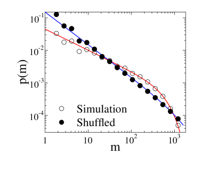
Figure 7: Distribution $p(m)$ of waiting times $m$ between consecutive records for fracture simulations and for the surrogate data. The bold lines represent best fit which was obtained using the generic functional form of Eq. (7). The value of the power law exponent is $z=0.62$ and $z=0.98$ for the simulated and shuffled data, respectively.

After a record occurred as the $n_{k}$th event of the sequence it gets broken by the next record which is the $n_{k+1}$th burst of the evolving system. The waiting time $m_{k}=n_{k+1}-n_{k}$ is an important characteristics of the dynamics, it provides the number of events one has to wait to break the $k$th record by the $(k+1)th$ one. The quantity $m_{k}$ is also called as the lifetime of the $k$th record. For IIDs it has been shown analytically that the probability distribution $p(m)$ of waiting times $m$ has a power law behavior

$$p(m)\sim m^{-z}$$ (8)

with a universal exponent $z_{IID}=1$. Figure 7 demonstrates that the lifetime distribution of the surrogate is consistent with the IID prediction with an exponent $z_{s}=0.98\pm 0.07$. For the fracture process the same functional form is obtained, however, with a different exponent $z=0.62\pm 0.03$. The low exponent $z<z_{IID}$ reflects the fact that during compressive failure of heterogeneous materials long waiting times between records more frequently occur than for a random sequence of IIDs. Since record breaking is controlled by the statistics of extremes, in a sequence of IIDs waiting times get larger with the record rank $k$, since it takes longer to break a larger record. However, in the fracture process large waiting times occur at the beginning, in spite of their larger size, records of higher rank may get broken faster because of the rapid increase of burst size when approaching failure.

The emergence of a characteristic record rank $k^{*}$ is further supported by the behavior of the average value of waiting times $m_{k}$. Figure 6$(c)$ presents the remarkable result that the record rank $k^{*}=7$ separates two qualitatively different regimes of the time evolution of the compressed system: at the beginning of the failure process $k<k^{*}$ the increasing waiting time implies a deceleration of record breaking, where it takes longer and longer to break the growing records.

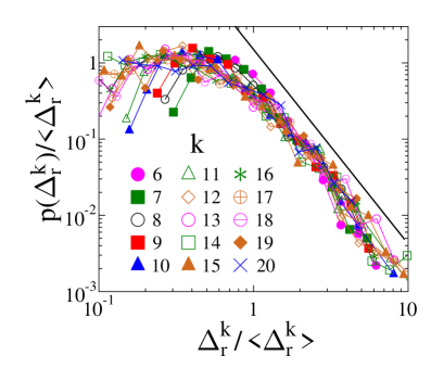
Figure 8: (Color online) Probability distribution $p(\Delta_{r}^{k})$ of record sizes $\Delta_{r}^{k}$ for fixed ranks $k$ rescaled with the average record size presented in Fig. 6$(a)$. Good quality collapse is obtained.

For IIDs the average waiting time must be monotonically increasing Shcherbakov et al. (2013) as observed in Fig. 6$(c)$ for the surrogate data set since records can be overcome after a larger and larger number of trials drawn from the same distribution. Comparing our simulation results to the IID findings, the increasing regime of $\left<m_{k}\right>$ can be attributed to the dominance of disorder in the fracture process consistent with our earlier findings Kun et al. (2013, 2014). Beyond $k^{*}$ the waiting time starts to decrease confirming the change of the dynamics. In spite of their larger size, records get broken after fewer and fewer small sized bursts which indicate the dominance of temporal and spatial correlations in triggering consecutive events.

In Ref. Kun et al. (2013) our simulations revealed the localization of breaking bursts to a damage band, which occurs at a characteristic strain value close to failure. Such localization has also been seen in acoustic emission data during laboratory experiments loaded at constant strain rate Lennartz-Sassinek et al. (2014). The spatial localization is accompanied by a rapid increase of the average burst size Kun et al. (2013, 2014). In Fig. 6$(d)$ the average strain $\left<\varepsilon_{k}/\varepsilon_{c}\right>$ where the records occurred is presented normalized by the critical strain of macroscopic failure. The strain range $\left<\varepsilon_{k}/\varepsilon_{c}\right>\approx 0.69-72$ corresponding to the record ranks $k^{*}=7-8$ is also highlighted in the figure. Comparing to the strain of localization $\left<\varepsilon_{k}/\varepsilon_{c}\right>\approx 0.85-0.9$ it follows that the acceleration of the RB process sets in significantly earlier. The macroscopic response of the system proved to be quasi-brittle, i.e. linearly elastic behavior is obtained where stronger non-linearity emerges solely close to failure due to the intensive bursting activity Kun et al. (2013, 2014). The yield stress $\sigma_{Y}$ and the corresponding strain $\varepsilon_{Y}$, which mark the onset of non-linearity of the constitutive curve $\sigma(\varepsilon)$, could be identified by computer simulations as $\sigma_{Y}/\sigma_{c}\approx 0.73$ and $\varepsilon_{Y}/\varepsilon_{c}\approx 0.7$, respectively. The characteristic strain $\left<\varepsilon_{k^{*}}/\varepsilon_{c}\right>$ of accelerated record breaking falls close to $\varepsilon_{Y}$.

To get a more detailed characterization of the evolution of the system towards failure, we evaluated the size distribution of records for fixed ranks $p(\Delta_{r}^{k})$. Figure 8 presents a scaling plot where distributions of different record ranks are rescaled with the average record size $\left<\Delta_{r}^{k}\right>$ presented in Fig. 6$(a)$. Except for the first few bins of the smallest record sizes good quality data collapse is obtained which implies the validity of the scaling structure

$$p(\Delta_{r}^{k})=\left<\Delta_{r}^{k}\right>\Phi(\Delta_{r}^{k}/\left<\Delta_{r}^{k}\right>),$$ (9)

where $\Phi(x)$ denotes the scaling function. The result demonstrates that records of different ranks have the same size distribution, they get only shifted to accommodate the increasing average size. Note that the functional form of the scaling function $\Phi(x)$ can be approximated as a power law for $x>1$. The slope of the straight line in Fig. 8 is 2.55. In the scaling analysis records of the lowest and highest ranks are not included because their size spans only a narrow range, and we do not have a sufficient number of events, respectively. When the event series is shuffled, any burst can be the first event, and hence, the first record. However, for higher ranks small size events have a very low chance to become a record. As a consequence the surrogate data set cannot have such a scaling behaviour because the functional form of the size distribution changes with the record rank: the size distribution of the first record is practically identical with the complete size distribution of bursts (see Fig. 5), while for higher record ranks the distribution must have a slower decay.

In Fig. 1 it has been highlighted that consecutive records enclose subsequences of the complete time series. To explore this further we analyzed how the size distribution $p(\Delta^{k})$ of these sub-sequences between the $k$th and $(k+1)$th records evolve as the system approaches failure. We excluded the two record bursts at the left and right hand sides of the sub-sequence from the statistics. Figure 9 presents the resulting size distributions $p(\Delta^{k})$ for several $k$ except for the lowest ranks ($k<5$) where event sizes span only a very narrow region so that no meaningful distributions could be obtained.

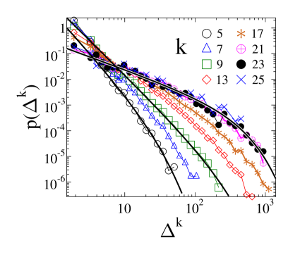
Figure 9: (Color online) Probability distribution $p(\Delta^{k})$ of burst sizes in sub-sequences of events between consecutive records. For demonstration three curves were fitted with the functional form Eq. (10). For the highest ranks $k\geq 20$ the distributions practically fall on the top of each other.

The distributions cannot be collapsed by rescaling with the average, only the cutoff of the distributions could be scaled on the top of each other. The reason is that the distributions have a power law functional form followed by an exponential cutoff,

$$p(\Delta^{k})\sim(\Delta^{k})^{-\tau_{k}}e^{-\Delta^{k}/\Delta^{k}_{s}}$$ (10)

however, the power law exponents $\tau_{k}$ are different for different record ranks $k$. It can also be observed in Fig. 9 that the cutoff scale $\Delta^{k}_{s}$ grows with the record rank $k$ and the curves of the highest ranks $k\geq 20$ fall practically on the top of each other. Figure 10 presents the exponent $\tau_{k}$ obtained by fitting with Eq. (10). For the lowest rank the exponent has a high value $\tau_{k}=3.26$ then it monotonically decreases and for the highest ranks it tends to the vicinity of $\tau_{k}=1.0$.

Figure 10: (Color online) The value of the exponent $\tau_{k}$ of the size distribution of sub-sequences of bursts between consecutive records as a function of the record rank $k$, together with the error bars.

The result is an interesting manifestation of the b-value anomaly Scholz (1968) (i.e. the change in the exponent of the log-linear frequency-magnitude distribution) we have pointed out before in DEM simulations of compressive failure Kun et al. (2013). In sub-sequences between records the number of events is practically equal to the waiting time $m_{k}$, which covers a broad range (see Fig. 6$(b)$). In the traditional analysis of the time series of bursts, event windows are considered with a fixed number (typically a few hundred) of events. This has the consequence that windows close to failure involve more and more records and sub-sequences which results in an exponent different from the one of single sub-sequences presented above Kun et al. (2013, 2014).

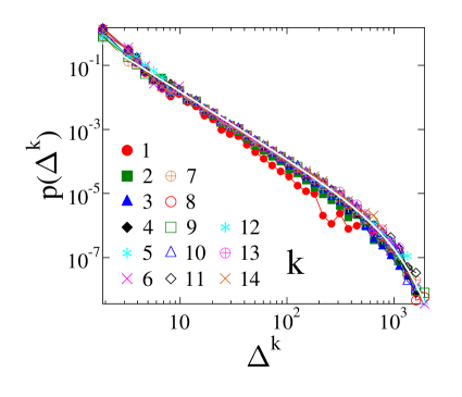
Figure 11: (Color online) Probability distribution $p(\Delta^{k})$ of burst sizes in sub-sequences of the shuffled event series between consecutive records. Except for the lowest ranks the curves fall on the top of each other. The white curve was obtained by fitting the functional form Eq. (10) with an exponent $\tau=2.1$ nearly equal to the one of the size distribution including all the bursts.

Figure 11 shows that no such behaviour exists when correlations are destroyed by shuffling the event series. Except for the lowest ranks, practically all the distributions of the sub-sequences fall on the top of each other. The emerging master curve can be well fitted with the functional form Eq. (10) where the exponent takes the value $\tau=2.1$ falling close to the size distribution exponent of the whole population of the bursts. The result is reasonable since all the sub-sequences are random samples of the complete event set.

VI Structure of the time series

Records are major events of the breaking activity of the compressed sample, which can have a strong effect on both the spatial and temporal occurrence of subsequent events. In Figure 1 the increasing value of the moving average of the burst size towards records may indicate some kind of precursory activity preceding record breaking events. In order to obtain a more detailed description of the internal structure of the time series we calculated the average size of bursts $\left<\Delta_{n}\right>$ before and after records of different ranks $k$ as a function of the event index $n-n_{k}$ relative to the records $n_{k}$. In Figure 12 zero index corresponds to the records while positive and negative values of $n-n_{k}$ stand for events preceding and following records, respectively. For clarity, the $\left<\Delta_{n}\right>$ curves are normalized by the average size $\left<\Delta_{r}^{k}\right>$ of the corresponding record.

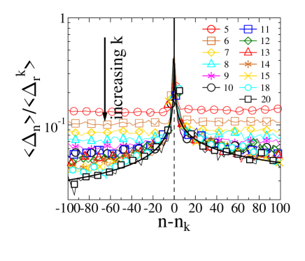
Figure 12: (Color online) Average size of events $\left<\Delta_{n}\right>$ in the vicinity of records as a function of their integer index relative to records $n-n_{k}$. High rank records are preceded by events of increasing size and they are followed by a relaxation process where the burst size gradually decreases. The bold line represents fit with Eq. (11).

It can be observed in Fig. 12 that low rank records just randomly pop up on a flat background without any signature of the imminent record event. However, high rank records are approached through a sequence of precursory events with an increasing average burst size, and they are followed by a relaxation process characterized by a gradually decreasing burst size. In this sense the later record-breaking events mimic the behaviour of the final dynamic rupture event. The functional form of $\left<\Delta_{n}\right>$ can be well fitted by an inverse power law

$$\left<\Delta_{n}\right>\sim\left|n-n_{k}\right|^{-\gamma}$$ (11)

on both sides of high rank records. In Figure 12 a best fit is obtained with the exponents $\gamma=0.38$ and $\gamma=0.31$ before and after records, respectively, considering the curves of $k=18,20$.

To characterize the temporal occurrence of events we analyzed in a similar way the average value of the physical waiting time $\left<T_{n}\right>$ between consecutive events before and after records as a function of the event index $n-n_{k}$ relative to record indices $n_{k}$. Figure 13 shows that for low record ranks $k<7$ the $\left<T_{n}\right>$ curves have a sharp local minimum at records which implies that the records are approached by a short period of increasing event rate and they are followed by a few relaxation events with increasing waiting times in between. However, for higher record ranks $k\geq 7$ the overall behavior drastically changes: The $\left<T_{n}\right>$ curves develop a broader and broader maximum at records which shows that large size events occurring in the vicinity of records (compare also to Fig. 12) are followed by longer waiting times. This behavior is the consequence of the strain controlled loading, i.e. after large size events it takes longer to build up again the stress field and initiate the next bursts. In a different context, studying the correlation of event size and the waiting time after events we have found analogous behavior in Ref. Kun et al. (2013, 2014). The present result is another form of appearance of the size-waiting time correlation.

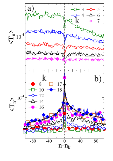
Figure 13: (Color online) Average value of the physical waiting time $\left<T_{n}\right>$ between consecutive events as a function of the event index relative to records $n-n_{k}$. The low and high rank records are presented separately in $(a)$ and $(b)$, respectively. The red bold continuous lines in $(b)$ represent fit with Eq. (11).

In the slow-down and acceleration periods the $\left<T_{n}\right>$ curves can be well fitted with the power law functional form. For the exponents providing best fit in Fig. 13 the same value 0.29 was obtained numerically on both sides of records.

VII Discussion

We investigated the statistics of record breaking bursts generated during the compressive failure of heterogeneous materials. A synthetic time series of crackling events was generated by discrete element simulations of a realistic model where a cylindrical sample was subject to uniaxial compression in a strain controlled way. Records of the time series of crackling events are identified as breaking bursts with size greater than any previous burst. The large system size in the model and the large number of samples generated by simulations allowed us to obtain high quality results for the statistics of records. In order to reveal the role of correlations of bursts the analysis was repeated for a surrogate time series which was generated by randomly reshuffling the simulated events. Additionally, our results were compared to the corresponding analytic findings on sequences of independent identically distributed random variables, as well.

The overall statistics of records is characterized by power law distributions of the size and lifetime of records and by the power law increase of the record number with the total number of events. This behavior deviates from the surrogate data set where correlations were destroyed, however, the later one agreed very well with the stationary process of IIDs.

As the compression proceeds the system gradually evolves towards macroscopic failure where the sample loses its integrity. We have shown earlier Kun et al. (2014, 2013) that the failure process has two qualitatively different stages: the beginning of the failure process is dominated by the structural disorder of the sample giving rise to an uncorrelated emergence of small sized breaking bursts. Later on as macroscopic failure is approached the fracture process accelerates which is indicated by the increasing burst size and by the decreasing waiting times between consecutive bursts. This second stage is dominated by the growing spatial and temporal correlations of local breaking events in the sample. In the present paper we showed that analyzing the statistics of record breaking bursts and their evolution with increasing rank, provides an alternative way for the quantitative characterization of the emerging correlations in the fracture process as the loaded system evolves towards failure.

Our analysis revealed the existence of a characteristic record rank $k^{*}$ which separates two regimes of the fracture process: for low record rank $k<k^{*}$ the process of record breaking slows down, i.e. it takes longer and longer to break a record. At $k^{*}$ the RB process starts to accelerate indicated by the rapidly decreasing record lifetime and by the increasing relative size increments of records. The surrogate event series proved to follow the IID predictions without any sign of the emergence of a characteristic record rank.

Records are found to affect the surrounding structure of the time series: approaching high rank records, bursts have a gradually increasing size separated by an increasing physical waiting time, while after records the event size decreases and the temporal occurrence accelerates with decreasing waiting times. The evolution of both the event size and waiting time is characterized by power law functional forms as a function of the distance from records. The result is consistent with our earlier finding presented in Ref. Kun et al. (2014), where the increase of waiting time after large size events has been pointed out by analyzing the size-waiting time correlation of bursts. The reason is the strain controlled loading, which has the consequence that larger events release the stress in a larger volume of the specimen, and hence, it takes longer to build up the stress field again and trigger the next burst.

Scaling analysis revealed that records of fixed ranks have the same size distribution which has power law asymptotics. Records split the time series of bursts into sub-sequences which typically contain fewer and fewer events as the system approaches macroscopic failure. We showed that bursts of sub-sequences are characterized by power law size distribution, however, the exponent spans a broad range decreasing to the vicinity of one towards failure. This result is consistent with the trend of the b-value anomaly of the time series Sammonds et al. (1992). In traditional b-value analysis of crackling time series windows of events are considered either with a fixed number of events or with a fixed strain or stress increment. Since records affect the structure of the time series, our analysis suggests that focusing on subsequences between records can provide significant additional and relevant information to that which can be inferred from the average properties of the time series of the whole population of all events. In principle this could improve forecasting power for catastrophic failure, but this depends on our being able to detect the processes revealed here in real time, and in a single realization, during a ’live’ experiment.

Our simulations were carried out with samples of about 100000 particles which corresponds to practically laboratory scale sample sizes. Comparison to simulations of a significantly smaller system size of 20000 particles (see Refs. Kun et al. (2014, 2013)) showed that in larger systems a larger number of crackling bursts are generated whose size spans a broader range. However, the probability distributions of the characteristic quantities of the event ensemble are quite robust, i.e. the value of the power law exponents are the same within the error bars. The same is valid for the number and size of records, however, for the value of the characteristic record rank $k^{*}$ no size dependence could be pointed out. In the simulations with 100000 particles the relative fluctuation of the total number of bursts is quite moderate (below 0.1). Tests of the effect of these fluctuations, e.g. by restricting the analysis to simulations where the number of bursts exceeds a threshold, revealed that they mainly affects the statistics of the results but no systematic bias occurred.

Our analysis strongly relies on the comparison of the record statistics of crackling noise time series to the corresponding IID findings and to the results of uncorrelated surrogates. A similar strategy has recently been applied in Ref. Shcherbakov et al. (2013) to study the avalanche dynamics of models of self organized criticality where IID results were derived by substituting the known steady state distribution of avalanche sizes into the generic IID formulas. Deviations of the record statistics of SOC models from the IID results were identified as signatures of correlations emerging in the dynamics of avalanches. Record breaking statistics of daily temperatures has proven a useful tool to investigate the effect of global warming. It has been pointed out in Ref. Redner and Petersen (2006) that the observed frequency and average value of record temperatures can be understood in terms of a stationary climate, so that the current warming rate does not have a noticable effect on the record statistics of daily temperatures (at least in the city of Philadelphia where the data was measured). Additionally, the ratio of the number of record high (record of the highest temperature of a given day) and record low (record of the lowest temperature of a given day) temperatures was suggested as a useful measure to point out trends in time series Redner and Petersen (2006). This idea was extended to earthquakes by Ref. Yoder et al. (2010) where the sequence of interval times between successive earthquakes were analyzed. It was shown that for global earthquakes the statistics of both record breaking longer and record breaking shorter intervals is consistent with IID processes. However, for an isolated aftershock sequence, where inter event times get systematically longer, the number of record breaking longer intervals was found to increase as a power law of the event number similarly to our result Eq. (4). At the same time the ratio $r$ of the number of record breaking longer and shorter intervals proved to be predominantly greater than one, which was suggested as a measure to distinguish between background seismicity and aftershock sequences Yoder et al. (2010). Extending the calculation of the ratio $r$ to a broader spatiotemporal interval, before and after the mainshock, $r<1$ and $r>1$ were found, respectively, which addressed a possibility of using record breaking statistics for forecastig Yoder et al. (2010). For inter event times of aftershocks the Omori-type relaxation was proved to be responsible for the power law increase of the number of records, while in our case the monotonically increasing average burst size towards failure plays a similar role. For earthquakes, the frequency-magnitude distributions for main shocks and aftershocks are the same, however, for fracture processes both the event magnitude and inter-event time exhibit a systhematic evolution towards macroscopic failure. In the present study we focused on the record breaking process of event magnitudes, the extension to inter-event times is a work in progress including also the analysis of the correlation of consecutive records Franke et al. (2012).