Representing model inadequacy: A stochastic operator approach

Abstract

Mathematical models of physical systems are subject to many uncertainties such as measurement errors and uncertain initial and boundary conditions. After accounting for these uncertainties, it is often revealed that discrepancies between the model output and the observations remain; if so, the model is said to be inadequate. In practice, the inadequate model may be the best that is available or tractable, and so it may be necessary to use the model for prediction despite its inadequacy. In this case, a representation of the inadequacy is necessary, so the impact of the observed discrepancy can be determined. We investigate this problem in the context of chemical kinetics and propose a new technique to account for model inadequacy that is both probabilistic and physically meaningful. A stochastic inadequacy operator $\mathcal{S}$ is introduced which is embedded in the ODEs describing the evolution of chemical species concentrations and which respects certain physical constraints such as conservation laws. The parameters of $\mathcal{S}$ are governed by probability distributions, which in turn are characterized by a set of hyperparameters. The model parameters and hyperparameters are calibrated using high-dimensional hierarchical Bayesian inference. We apply the method to a typical problem in chemical kinetics—the reaction mechanism of hydrogen combustion.

65C50, 62F15

1 Introduction

Model inadequacy is a complex and critical issue that affects nearly all realms of computational science and engineering. In general, models of physical systems are imperfect: they rely on abstractions and simplifications which do not perfectly represent the modeled system. Sometimes the imperfections are small enough that any discrepancy between the model and reality is dominated by observation error, such that the discrepancy is essentially undetectable given existing measurement technology. In contrast, a model is demonstrably inadequate when the imperfections lead to a detectable inconsistency between the model and observations. Such inadequacies are often detected during model validation, which is the process of assessing whether a given mathematical model, including representations of relevant uncertainties, is consistent with knowledge regarding the modeled system [3, 5, 46]. When an inadequacy is detected, one would generally prefer to improve the model to remove the discrepancy, but such improvement is often not feasible.

One of the most important uses of computational models is to make predictions, by which we mean to predict values of model outputs without corroborating observations of the predicted quantities. Such predictions are important to engineering design and decision making. If one is using an inadequate model, as is often the case because that is all that is tractable, it is important to characterize the uncertainty in the prediction due to model errors [46]. A representation of model inadequacy is therefore needed, and it is critical that the model inadequacy be represented in a way that will allow the uncertainty to be propagated to the predictions, as described by [46].

Treatment of model inadequacy has been a topic of research in the Bayesian statistics literature for a number of years. A common approach is to pose and calibrate a purely statistical representation of the discrepancy between the model output and the true value of that output (often called a bias function) [34, 5, 29, 30, 58]. However, this representation is unable to characterize the impact of inadequacy on predictions of an unobserved quantity [46]. Further, we generally have both qualitative and quantitative knowledge about the phenomena being modeled, the reasons for the model inadequacy and the way errors are injected into the model. It is important to formulate the inadequacy formulation to respect this knowledge if it is to reliably represent the uncertainty in the predictions. Oliver et al [46] developed such an inadequacy representation for a trivial example, but broadly applicable techniques for formulating inadequacy representations for models of complex physical systems are not available.

We propose a new broadly applicable formulation for model inadequacy in terms of stochastic operators, which can satisfy the requirements above. Here, this approach is applied to models of chemical kinetics as an example of a relatively complex system with inadequate models and rich knowledge regarding the phenomenon. Specifically, the stochastic model inadequacy operator is introduced as a source in the equations describing the evolution of the chemical system, and is constructed to respect certain non-negotiable constraints on the system. This approach results in a model inadequacy representation that is both probabilistic and physically meaningful. The formulation is demonstrated on a typical problem in chemical kinetics, namely the reaction mechanism model for hydrogen combustion, where it is shown that the formulation is flexible enough to account for significant inadequacies present in the original model.

Chemical mechanisms and kinetics models describe the process and rates of chemical reactions [57, 61]. In general, a reaction mechanism is extraordinarily complex, even when there are only two or three initial reactants. An accurate description of the chemical processes involved in the oxidation of hydrocarbons, for example, may include hundreds or thousands of reactions and fifty or more chemical species [54, 59]. At the same time, there is significant uncertainty in the reaction rates for these reactions; recent efforts to address this include [35, 39, 10]. Furthermore, kinetics models of these chemical mechanisms must be embedded within a larger fluids calculation to model practical combustion systems. The chemical dynamics must then be represented at every point in space and time. Because the computational cost of such detailed mechanisms is so high, drastically reduced mechanisms are often used instead. Such reduced models are commonly found in the combustion literature [12, 59, 62]. However, errors introduced by the reduced models may render the model inadequate even if the detailed model it is based on is not. Alternatively, it may be that a highly accurate detailed reaction mechanism is not known, in which case any available model should be viewed as a reduced mechanism relative to the unknown reality. This work is concerned with accounting for the inadequacy resulting from the use of a reduced chemical mechanism, though the representation proposed is equally applicable to inadequate mechanisms.

If a chemical kinetics model is inadequate, it would be best to improve the kinetics model directly to eliminate the inadequacy. Indeed, refinement of chemical mechanisms in combustion is an active topic of research; for a small sample focused on H₂/O₂ reactions, see [11, 12, 17, 42]. However, this type of refinement is not always an option, because of a lack of physical insight required to develop a higher fidelity model, a lack of detailed observational data to support such model development, or a lack of time or other resources required for the model development process. Further, even when a higher fidelity model exists, it may be impractical to use due to a lack of the necessary computational resources. Thus, there is a general need for methods that account for the discrepancy between the inadequate model and the observations that do not require traditional model improvement. To develop such a representation, one must adopt a mathematical framework for reasoning about the model inadequacy. Here we adopt a Bayesian point of view [19, 31], and thus, any lack of knowledge—and model inadequacy specifically—is modeled using probability. Further, the Bayesian approach offers a natural framework for representing all uncertainties that arise in using reduced kinetics models to make predictions—including modeling inadequacy of course but also uncertain kinetics parameters and measurement uncertainties—as well as a natural method for updating these representations to incorporate information from data [16, 32, 13, 53].

In this work, inadequacy representations are formulated not as corrections of the model output, but as stochastic enrichments of the model itself which are specifically constructed to respect known physical constraints. A set of chemical reactions is modeled by describing the time derivative of the species concentrations and temperature, so the model consists of a set of nonlinear ordinary differential equations. The necessary constraints in this context are conservation of atoms, conservation of energy, and non-negativity of concentrations. The model inadequacy representation developed here is characterized by a stochastic operator $\mathcal{S}$, which is added to the formulation of the time derivatives of the species concentrations and temperature. This operator is constructed such that all realizations of the solution of the enriched reduced model—i.e. the reduced model coupled with the inadequacy representation—conserve atoms and energy and have non-negative concentrations at all times. The main component of the operator is additive, linear, and probabilistic, encoded in a random matrix $S$. The use of the term random matrix implies that each entry is characterized by a probability distribution. This usage is consistent with the definition of random matrices from random matrix theory (see [21, 38]), although in that field a random matrix is usually much less constrained than in the present case, and its properties (such as the distributions of the eigenvalues) are found in the limit as the size of the matrix goes to infinity. A few applications of random matrices to engineering problems are presented by Soize [55, 56]. However, this work also differs from our approach in that the probability of a given matrix is characterized by properties of the entire matrix, such as the determinant, whereas we characterize each non-zero entry. Moreover, the inadequacy operator $\mathcal{S}$ is more general than a random matrix alone, including two nonlinear operators as well.

Other stochastic formulations for chemically reacting systems have appeared in the literature. Of particular interest here is the approach pioneered by Gillespie [27], in which a stochastic model is formulated to represent aleatory uncertainty introduced by, for example, quantum indeterminacy. These ideas have found important applications in systems where the populations of molecules involved is small so that the effects of these aleatory uncertainties can lead to substantial deviations from classical deterministic models, such as gene regulatory networks [33]. However, the goals of this approach are fundamentally different from those pursued here. In particular, the Gillespie approach seeks to enhance the physical description of chemical kinetics to account for non-deterministic physical processes. In contrast, it is assumed here that the evolution of the species concentrations is in fact deterministic—i.e., that the species populations are sufficiently large that the stochastic effects represented by Gillespie are negligible—but that an entirely satisfactory deterministic model is either unavailable due to lack of knowledge or computationally intractable.

Although the goals are quite different, the approach is similar in that the classical deterministic description of chemical kinetics is replaced by a stochastic description in which the species concentrations are random variables. However, the form of stochasticity in typical stochastic kinetics is overly restrictive for the current purposes. For example, in a common stochastic kinetics approach, the model takes the form of the chemical Langevin equation, in which the deterministic kinetics model is modified by an additive white noise term. In this case, the noise only modifies the source terms for species appearing in the original deterministic model. When applied to the inadequate deterministic models considered here, this formulation cannot account for atoms that belong to species that are not tracked as part of the inadequate model and thus cannot fully capture the inadequacy. In general, a richer representation of the inadequacy—one that accounts for both missing species and reaction pathways—is required. Such a form is proposed in this work.

The proposed form of the inadequacy representation satisfies all the constraints implied by conservation of atoms, conservation of energy, and non-negativity of concentrations. However, satisfying these constraints does not fully determine the stochastic inadequacy operator. The stochastic elements of the operator are described by hyperparameters that determine their mean and variance, and these can only be determined by reference to the actual discrepancy between the model and the real system, which is accomplished through a process of calibration. Further, just like any other model, the model enriched with its inadequacy representation must be validated against observations of the system.

The calibration and validation of models of physical systems has been a subject of great interest in computational science and engineering [43, 52, 44]. Generally, calibration is an inverse problem in which model parameter values are inferred given data on outputs from the model. In the presence of uncertainty, such an inverse problem is naturally posed in terms of Bayesian inference. With uncertainties, the validation question of whether the model is consistent with the data is recast as a question whether it is improbable that the data could arise from the model, and a variety of statistical tests are available to measure that. The approach pursued here is essentially posterior predictive assessment as described by [25, 48] and by [41] for models of physical systems. These and similar calibration and validation techniques have been applied in a wide variety of applications, including turbulence [45, 15], kinetics [50], atomistic systems [22], flow in porous media [4], fatigue crack growth [49], and cardio-vascular flows [51], to name just a few.

Returning to the inadequacy representation considered here, the hyperparameters characterizing the stochastic inadequacy operator need to be calibrated as discussed above. Because the inadequacy operator is stochastic, the forward problem mapping specific values of the hyperparameters to the model outputs is also stochastic. This complicates the Bayesian inverse problem. A hierarchical Bayesian formulation is used to address this [7].

The rest of the paper is organized as follows. In §2, we give a brief overview of kinetics modeling. In §3, the general formulation and properties of the stochastic operator are presented. §4 describes the Bayesian framework for calibration and validation of the various models, including hierarchical Bayesian modeling and validation under uncertainty. In §5, the approach is applied to the specific case of hydrogen combustion. Concluding remarks are given in §6.

2 Chemical mechanism models

Chemical mechanisms and kinetics models describe the process and rates of chemical reactions. In a typical chemical reaction, there is a set of reactant species which, after a complex series of intermediate reactions, ultimately form the chemical products. These intermediate steps, in which chemical species react directly with each other, are called elementary reactions. The set of elementary reactions is called the reaction mechanism, and a typical combustion problem may include tens to thousands of elementary reactions. This section provides a minimal introduction to the essentials of chemical kinetics necessary to understand the development of the model inadequacy representation in §3. For more details on chemical kinetics, see [57] for a general text and [61] for a presentation focused on combustion.

To introduce the main concepts, consider the following example reaction set with four species and two reversible elementary reactions:

$$\cee{A+B<=>[k_{1}^{f}][k_{1}^{b}]C},\quad\quad\cee{A+C<=>[k_{2}^{f}][k_{2}^{b}]D},$$

where A, B, C, and D denote the different chemical species, and $k_{1}^{f}$, $k_{2}^{f}$ and $k_{1}^{b}$, $k_{2}^{b}$ are the forward and backward rate coefficients, respectively. Let $\bm{x}=[x_{1},x_{2},x_{3},x_{4}]^{T}$ be the vector of molar concentrations (having dimensions moles per unit volume) corresponding to species A, B, C, D. The rate of each reaction is often modeled as linear in the concentration of the reactants, although this power, or order, associated with a given species may be non-unity. With the assumption of linearity in each species, the forward rate expressions of the two reactions are thus

$$r_{1}^{f}=k_{1}^{f}x_{1}x_{2},\quad\quad r_{2}^{f}=k_{2}^{f}x_{1}x_{3}.$$

Similarly, the backward rates are given by

$$r_{1}^{b}=k_{1}^{b}x_{3},\quad\quad r_{2}^{b}=k_{2}^{b}x_{4}.$$

Finally, the ODEs for the molar concentrations are

$$\dot{x}_{1} =-r_{1}^{f}+r_{1}^{b}-r_{2}^{f}+r_{2}^{b}$$

$$\dot{x}_{2} =-r_{1}^{f}+r_{1}^{b}$$

$$\dot{x}_{3} =+r_{1}^{f}-r_{1}^{b}-r_{2}^{f}+r_{2}^{b}$$

$$\dot{x}_{4} =+r_{2}^{f}-r_{2}^{b}.$$

The rate coefficients $k$ are generally functions of temperature, and may follow a given empirical form depending on the specific reaction. A common form is the Arrhenius Law, $k(T)=Ae^{-E/(R^{\circ}T)}$, for some prefactor $A$, activation energy $E$, and universal gas constant $R^{\circ}$. Another common form is the modified Arrhenius, $k(T)=AT^{b}e^{-E/(R^{\circ}T)}$, with the additional constant $b$. These expressions are often used in the literature to describe the forward rate coefficient, and this is true in the example problem in §5. However, the backwards rate coefficients are usually not specified. Instead, these are determined from the equilibrium constant which depends only on the thermodynamics of the reaction. See [57] for details.

Given a reversible reaction and the forward rate coefficients, there are various software libraries which will solve for the backwards rate coefficients. In this work, a chemistry software library called Antioch (A New Templated Implementation of Chemistry for Hydrodynamics) was used to set up the chemical model, query thermodynamic information, and solve for the reverse reaction rates [1].

To complete the specification of the system, a governing equation for temperature is required. This equation is derived based on conservation of energy. In this work, we consider a reacting mixture of ideal gases. Further, the reactions are assumed to occur in a constant volume that does not exchange heat or mass with its surroundings. In this case, changes in the system temperature are due only to the difference in chemical energy between the reactants and products. For an ideal gas, the internal energy depends only on temperature (not $v$ or $p$) and the species concentrations:

$$U(T,\bm{x})=\sum_{i}u_{i}(T)x_{i}.$$

Thus,

$$\frac{dU}{dt}=\sum_{i}{\frac{\partial u_{i}}{\partial t}x_{i}+u_{i}\frac{\partial x_{i}}{\partial t}}=\sum_{i}{c_{v_{i}}\frac{\partial T}{\partial t}x_{i}+u_{i}\frac{\partial x_{i}}{\partial t}}=\frac{\partial T}{\partial t}\sum_{i}{c_{v_{i}}x_{i}+u_{i}\frac{\partial x_{i}}{\partial t}}.$$

Since the volume is constant—i.e., no work is done on the system—and no heat is added, the change in the energy $U$ must be zero. Setting $dU/dt$ to zero and solving for $dT/dt$ yields

$$\frac{dT}{dt}=-\left(\frac{1}{\sum_{i}{c_{v_{i}}x_{i}}}\right)\left(\sum_{i}{u_{i}\dot{x}_{i}}\right).$$

Note that $\frac{dT}{dt}$ is a function of both the molar concentrations and their time derivatives. The representations of the remaining functions $c_{v_{i}}(T)$ and $u_{i}(T)$ may be found in the literature, generally as seven or nine term polynomials. The commonly used NASA polynomials are used in this work [37].

With the time derivative of temperature, the mathematical model of the reaction mechanism is complete. To summarize, there is an ODE for the time derivative of each species and also for temperature. These can be written more compactly as

$$[\dot{x}_{1},\dot{x}_{2},\dots,\dot{x}_{n},\dot{T}]^{T}=\mathcal{F}(\bm{x},\dot{\bm{x}},T)$$

where $\mathcal{F}$ is a nonlinear operator acting on the state $(\bm{x},T)$ and the time derivatives of $\bm{x}$. Note that $\mathcal{F}$ depends on $\dot{\bm{x}}$ only through the energy equation.

3 Formulation of the model inadequacy

In contrast to the simple example mechanism in §2, mechanisms describing complex chemical systems like those encountered in combustion often include hundreds of reactions. One of the standard models for methane combustion, for example, includes fifty-three species and 325 reactions [54]. Such models are often referred to as detailed mechanisms and will be written here as $\mathcal{D}(\bm{x}^{D},\dot{\bm{x}}^{D},T)$. In the context of a reacting flow simulation, such a large mechanism may be too computationally expensive to be practical, and thus it is common to use a reduced chemistry model consisting of a subset of the species and reactions from the detailed model.

To be concrete, suppose that the detailed model includes $n_{D}$ species and $m_{D}$ reactions. Further suppose that the reduced model includes $n_{R}$ species and $m_{R}$ reactions, where $n_{R}\leq n_{D}$ and $m_{R}<m_{D}$. The reduced model always contains fewer reactions than the detailed; the number of species included in the reduced model may or may not be smaller, although in practice it is almost always true that $n_{R}<n_{D}$. The reduced model is denoted $\mathcal{R}(\bm{x}^{R},\dot{\bm{x}}^{R},T)$.

In the case that the reduced model does not adequately represent the detailed (or the real chemical reaction), one has two options: (1) improve the reduced model directly with a more accurate mechanism, or (2) incorporate a representation of the model error of the reduced model. As noted in §1, it is often impractical to improve the model and thus, the focus of this work is on developing a generally applicable model inadequacy representation for reduced chemistry models. The model inadequacy is represented by a stochastic operator $\mathcal{S}$ that is appended to the reduced model $\mathcal{R}$, as indicated in Figure 1, which shows the progression from the detailed model to the proposed stochastic model.

Figure 1: Relationship between the detailed model, deterministic reduced model, reduced model with general model inadequacy representation, and reduced model with stochastic operator model inadequacy representation.

In the figure, the $\mathcal{D}$ and $\mathcal{R}$ operators correspond to the deterministic detailed and reduced models introduced above. The operator $\mathcal{R}^{G}$ denotes the reduced mechanism used with a general stochastic inadequacy model, $\mathcal{G}_{\omega}$, where $\omega$ is a set of random variables. For example, $\mathcal{G}_{\omega}$ could be a purely statistical model that is trained based on observations of the detailed model reaction rates. On the other hand, this term could represent an augmentation of the chemical mechanism obtained by incorporating more reactions from the detailed model. In this case, the model inadequacy representation would in fact be deterministic (with $\omega=\{\}$). This approach would necessitate more information about the true chemical reaction than we expect to have or are willing to use and thus is not generally applicable.

Here we take an approach which is intermediate between a strictly statistical representation and a strictly physics-based approach. Physics is incorporated into the approach in that we insist that the inadequacy representation respect certain known features of the system, but, since our knowledge of the true dynamics is incomplete, the model is necessarily stochastic, implying that there is a range of behaviors consistent with our knowledge. In the chemical kinetics case, we know that errors in the model are due to unrepresented species and unrepresented pathways by which species transform into each other. Further, both atoms and energy must be conserved and species concentrations and temperature must remain non-negative. To account for the effects of the missing species and reactions and to satisfy these constraints, a stochastic operator representation of the inadequacy is posed, as shown on the bottom left of Figure 1. The reduced model $\mathcal{R}^{S}$ plus the stochastic inadequacy operator $\mathcal{S}$ is called the operator model $\mathcal{O}$. Note that the the physical basis of the inadequacy representation gives structure to the operator, while the statistical aspect gives it the flexibility needed to represent the error over a wide range of conditions and allows it to be calibrated to data.

For clarity of notation, the superscripts ($D$, $R$, $G$, $S$) on either the state vector $\bm{x}$ or the reduced model $\mathcal{R}$ are included to reflect the model at hand. As will become clear, to satisfy the requirements mentioned above, the inadequacy formulation alters the state vector $\bm{x}$ and the reduced model operator $\mathcal{R}$, so $\bm{x}^{S}$ and $\mathcal{R}^{S}$ differ from the corresponding $\bm{x}^{R}$ and $\mathcal{R}$.

3.1 Components and State Variables of the Operator Model

3.1.1 Components of the operator

The main action of the inadequacy operator $\mathcal{S}$ is to modify the time derivatives of the species concentrations. The operator consists of three pieces: a random matrix $S$, a nonlinear operator $\mathcal{A}$, and a nonlinear operator $\mathcal{W}$. The random matrix $S$ is intended to represent the most general linear correction that can be made to the reduced chemistry model. However, to ensure sufficient flexibility for mass to move between species, it is necessary to introduce a nonlinear operator $\mathcal{A}$, as discussed in §3.4. The final piece of the operator accounts for conservation of energy and is denoted $\mathcal{W}$.

Note that $S$ and $\mathcal{A}$ act on just the concentrations, while $\mathcal{W}$ acts on the concentrations and their derivatives. Moreover, it is convenient to formulate $S$ in terms of atomic concentrations, while $\hat{S}$ denotes the corresponding matrix in terms of molar concentrations. This section focuses on $S$ instead of $\hat{S}$ because many of the properties of the matrix (such as non-positivity of eigenvalues) are better expressed in terms of atoms instead of moles (see §B). To map between $S$ and $\hat{S}$, the vector $\bm{l}$ is used, whose $i$th entry counts the number of atoms (of all types) in one molecule of the $i$th species. For example, if the set of species is H₂, O₂, H, O, OH, H₂O, then $\bm{l}=[2,2,1,1,2,3]$. Let $L$ denote the square matrix with the entries of $\bm{l}$ on the diagonal. Then $\hat{S}=L^{-1}SL$ applies to molar concentrations. Finally, putting the three pieces together,

$$\mathcal{S} =\hat{S}+\mathcal{A}+\mathcal{W}$$

$$=L^{-1}SL+\mathcal{A}+\mathcal{W},\quad\text{or more explicitly,}$$

$$\mathcal{S}(\bm{x}^{S},\dot{\bm{x}}^{S},T) =L^{-1}SL\bm{x}^{S}+\mathcal{A}(\bm{x}^{S})+\mathcal{W}(\bm{x}^{S},\dot{\bm{x}}^{S},T).$$

3.1.2 Augmentation of the state vector

The reduced model tracks fewer species than the detailed model. It should be possible then, for the inadequacy formulation to represent this difference. However, we do not want to include all the extra (missing) species in the inadequacy representation. Therefore, in order to account for the missing species in the reduced model, the state space is augmented by entries for all types of atoms. These entries are referred to as catchall species and act as a sort of pool of each atom type, representing atoms bound in unrepresented species. The presence of the catchall species allows the operator $\mathcal{S}$ to move atoms to and from these pools instead of constraining every atom to one of the species of the reduced model, which is overly restrictive because in the detailed model, atoms may move to species that are not part of the reduced model. Thus, $\bm{x}^{S}$ is of length $n_{S}=n_{R}+n_{\alpha}$, where $n_{\alpha}$ is the number of atom types, and is of the form

$$\bm{x}^{S}=[x_{1},\dots,x_{n_{\alpha}},x_{n_{\alpha}+1},\dots,x_{n_{\alpha}+n_{R}}]^{T}.$$

We denote the catchall species of element $\mathbb{X}$ by $\mathbb{X}^{\prime}$. For example, consider a reduced model that includes H₂, O₂, OH, and H₂O. Then the catchall species are H^′ and O^′, and

$$\bm{x}^{S}=[x_{1},x_{2},x_{3},x_{4},x_{5},x_{6}]^{T}$$

where $x_{1},\dots,x_{6}$ corresponds to H^′, O^′, H₂, O₂, OH, and H₂O, in that order.

The introduction of the catchall species raises an important point about the structure of the reduced model: it takes on a different form when used in conjunction with the stochastic operator $\mathcal{S}$. Because of this fact, the reduced model used with the stochastic operator is denoted by $\mathcal{R}^{S}$ to distinguish it from the original reduced model $\mathcal{R}$. There are two differences between these operators. First, $\mathcal{R}^{S}$ acts on a vector space of dimension $n_{S}$ rather than $n_{R}$, although it has no effect on the first $n_{\alpha}$ entries of $\bm{x}^{S}$ (i.e., the catchall species). Second, because the effect of the catchall species on the energy equation is not additive, the differential equation for $T$ is removed from $\mathcal{R}^{S}$, and the entire calculation is accounted for with $\mathcal{W}$.

3.2 Physical constraints and their implications

There are two non-negotiable constraints that any physically realistic model of the system at hand must respect: (I) conservation of atoms, and (II) non-negativity of concentrations. This ensures that the inadequacy operator respects physical laws that are known to be true for the systems of interest. This section develops the implications of these constraints for the components of the operator $\mathcal{S}$ with a focus on the matrix $S$ since, as will be shown, $\mathcal{A}$ and $\mathcal{W}$ are subsequently chosen to take forms that are known to satisfy these constraints.

3.2.1 Conservation of atoms

To enforce (I), first let $E=[e_{ij}]$ be the $n_{\alpha}\times n_{S}$ matrix where $e_{ij}$ is the fraction of atoms of type $i$ in one molecule of species $j$. Then $ESL\bm{x}^{S}$ is the rate of change of the number of each atom due to the operator $S$. Because atoms are conserved $ESL\bm{x}^{S}$ must be zero, which implies that $ES=0$.

To continue the example shown in §3.1, consider the case with atom types H and O, and species H^′, O^′, H₂, O₂, OH, H₂O. Then matrix $E$ takes the form:

$$E=\begin{bmatrix}1&0&1&0&1/2&2/3\\ 0&1&0&1&1/2&1/3\end{bmatrix}.$$

To satisfy the constraint that $ES=0$, the matrix $S$ is constructed according to

$$S=CP,$$

where $C$ is a deterministic matrix and $P$ is probabilistic. The roll of the matrix $C$ is to ensure conservation of atoms, while $P$ is constructed to ensure that the concentrations are non-negative. To guarantee conservation of atoms, the columns of $C$ must span the nullspace of $E$, i.e. $\text{span}(C)=\text{null}(E)$. Thus,

$$ES=ECP=(EC)P=0\cdot P=0.$$

$E$ is of dimension $n_{\alpha}\times n_{S}$, so the dimension of the nullspace is $n_{S}-n_{\alpha}=n_{R}$. Thus $C$ is of dimension $n_{S}\times n_{R}$ and $P$ is of dimension $n_{R}\times n_{S}$.

3.2.2 Non-negativity of concentrations

The second constraint (II) is that the concentrations must not be negative. To see how to enforce this, consider the differential equation for species $\mathbb{X}_{i}$:

(1) $$\dot{x}_{i}=(\mathcal{R}^{S}(\bm{x},\bm{T}))_{i}+(\mathcal{S}(\bm{x}))_{i}=(\mathcal{R}^{S}(\bm{x},\bm{T}))_{i}+(L^{-1}SL\bm{x})_{i}+(\mathcal{A}(\bm{x}))_{i}.$$

We must ensure that $\dot{x}_{i}\geq 0$ when $x_{i}=0$ for $i=1,\dots,n_{S}$. The first term of the RHS of (1) is not a problem, as this is the nonlinear part from the reaction mechanism and is thus already physically consistent [23]. The same argument holds for $\mathcal{A}(\bm{x})$ because it takes the form of a standard chemical reaction model, as will be shown in §3.4. Note that the energy operator $\mathcal{W}$ is not written above because it does not modify the derivative of $x_{i}$.

Finally, the second term must satisfy the constraint. Although the constraint is naturally posed here in terms of molar concentrations, it is helpful to rephrase this in terms of atomic concentrations. One can show that the constraint is satisfied for moles if and only if it is satisfied for atoms:

$$L^{-1}SL\bm{x}\geq 0\quad\iff\quad S\bm{y}\geq 0.$$

To prove this, consider the $i$th entry of $L^{-1}SL\bm{x}$:

$$(L^{-1}SL\bm{x})_{i} =L^{-1}\sum_{j}s_{ij}l_{j}x_{j}$$

$$=\frac{1}{l_{i}}\sum_{j}s_{ij}l_{j}x_{j}$$

but $l_{j}x_{j}=y_{j}$ and all $l_{i}>0$, $i=1,\dots,n_{S}$. Thus,

$$\frac{1}{l_{i}}\sum_{j}s_{ij}l_{j}x_{j}\geq 0\iff\sum_{j}s_{ij}y_{j}\geq 0.$$

But the final term is exactly the $i$th element of $S\bm{y}$.

Continuing in terms of the atomic concentrations, the $i$th component of $S\bm{y}$ is given by

(2) $$(S\bm{y})_{i}=s_{ii}y_{i}+\sum_{j\neq i}s_{ij}y_{j}.$$

The first term from the diagonal, $s_{ii}y_{i}$, automatically respects the constraint: $s_{ii}$ may be set to be any constant value, since then $s_{ii}y_{i}\rightarrow 0$ as $y_{i}\rightarrow 0$. To enforce the constraint, it must be that the sum, $\sum_{j\neq i}s_{ij}y_{j}$, is non-negative. But this sum does not depend on $y_{i}$, so we choose to set $s_{ij}\geq 0$ for all $i\neq j$. This could be made less restrictive by incorporating information from the nonlinear system, i.e. set ($\mathcal{R}^{S}(\bm{x}))_{i}+\sum_{j\neq i}\hat{s}_{ij}x_{j}\geq 0$, but this would violate the linearity assumption on $S$. It would also necessitate using information from the reduced model, whereas we aim to constrain the inadequacy operator independently of $\mathcal{R}$.

3.2.3 Sparsity of $S$

In practice, many of the entries of $S$ are identically zero. In theory, $S$ could be completely dense if every species included every type of atom. However, this generally does not occur in practical combustion reactions. The following proves which entries of $S$ are identically zero, using an argument based on the zeros of the matrix $E$.

Theorem 3.1.

Consider the $i$th row of $E$. Let $\mathcal{J}_{i}=\{j|e_{ij}\neq 0\}$ and $\mathcal{J}_{i}^{c}=\{j|e_{ij}=0\}$. Then every element $s_{jk}=0$ for $j\in\mathcal{J}_{i}$ and $k\in\mathcal{J}_{i}^{c}$.

Proof 3.2.

Consider the $i$th row of $E$ and the $k$th column of $S$. Since $ES=0$, we have

(3) $$0=\sum_{j}e_{ij}s_{jk}=\sum_{j\in\mathcal{J}_{i}}e_{ij}s_{jk}+\sum_{j\in\mathcal{J}_{i}^{c}}e_{ij}s_{jk}=\sum_{j\in\mathcal{J}_{i}}e_{ij}s_{jk}+0.$$

But since $j$ and $k$ are in disjoint sets, the sum in line (3) does not include the diagonal term $s_{jj}$. But the diagonal term is the only negative value in the $k$ column. Thus, all $s_{jk}=0$, where $j\in\mathcal{J}_{i}$ and $k\in\mathcal{J}_{i}^{c}$.

For another method to determine the sparsity of $S$, see Appendix B. In addition to sparsity, the constraints on $S$ imply that it has non-positive eigenvalues. See Appendix B for more details.

3.3 Construction of the matrix $S$

The structure of $S$ is now clear; the next step is to actually construct it. The challenge in this construction is that both constraints must be simultaneously satisfied by any realization of $S$. This subsection presents a method for construction of the operator. To help demonstrate the upcoming matrix decompositions and inequality constraints, the construction will also be shown for the example set of species (H^′, O^′, H₂, O₂, OH, H₂O). In this case, $S$ has the form

$$S=\begin{bmatrix}s_{1,1}&0&s_{1,3}&0&s_{1,5}&s_{1,6}\\ 0&s_{2,2}&0&s_{2,4}&s_{2,5}&s_{2,6}\\ s_{3,1}&0&s_{3,3}&0&s_{3,5}&s_{3,6}\\ 0&s_{4,2}&0&s_{4,4}&s_{4,5}&s_{4,6}\\ 0&0&0&0&s_{5,5}&s_{5,6}\\ 0&0&0&0&s_{6,5}&s_{6,6}\end{bmatrix},$$

where the diagonal elements are non-positive and the off-diagonal elements are non-negative. Here, $n_{R}=4$, $n_{\alpha}=2$.

First, $C$ is formed to span the nullspace of $E$. To accomplish this, let the bottom $n_{R}\times n_{R}$ block of $C$ be the identity matrix $I_{n_{R}}$. The remaining top $n_{\alpha}$ rows will be the negative of the last $n_{R}$ columns of $E$. Let this matrix block be denoted $E^{*}$. Note that every element of $E^{*}$ is non-positive. Thus, $C$ has the form

$$C=\left[\begin{array}[]{c}E^{*}\\ \hline\cr I_{n_{R}}\end{array}\right].$$

Since $E=[I_{n_{\alpha}}|-E^{*}]$, it is clear that $EC=0$.

For the H₂/O₂ example at hand,

$$E=\begin{bmatrix}1&0&1&0&1/2&2/3\\ 0&1&0&1&1/2&1/3\end{bmatrix}.$$

Thus,

$$E^{*}=\begin{bmatrix}-1&0&-1/2&-2/3\\ 0&-1&-1/2&-1/3\end{bmatrix}$$

and

$$C=\begin{bmatrix}-1&0&-1/2&-2/3\\ 0&-1&-1/2&-1/3\\ 1&0&0&0\\ 0&1&0&0\\ 0&0&1&0\\ 0&0&0&1\end{bmatrix}.$$

Next, we construct the $n_{R}\times n_{S}$ random matrix $P$. The first step is to specify which entries are non-negative, non-positive, or strictly zero. Then, by taking advantage of the special structure of $C$, it is possible to transfer the inequalities placed on the entries of $S$ to those of $P$. Let $P_{1}$ contain the first $n_{\alpha}$ columns of $P$, and $P_{2}$ the remaining $n_{R}$ columns. So far we have

$$S =CP$$

(7) $$=\left[\begin{array}[]{c}E^{*}\\ \hline\cr I_{n_{R}}\end{array}\right]\left[\begin{array}[]{c|c}P_{1}&P_{2}\end{array}\right]$$

(10) $$=\left[\begin{array}[]{c|c}E^{*}P_{1}&E^{*}P_{2}\\ \hline\cr I_{n_{R}}P_{1}&I_{n_{R}}P_{2}\end{array}\right]$$

(13) $$=\left[\begin{array}[]{c}E^{*}P_{1}|E^{*}P_{2}\\ \hline\cr I_{n_{R}}P\end{array}\right].$$

The bottom row of (13) shows how to transfer the inequalities from matrix $S$ to $P$. Since $P$ is left-multiplied by the identity matrix, it must be that the signs match for the corresponding elements of $S$. In particular, for $1<i\leq n_{R}$ and $\forall j$, then

(14) $$p_{i,j} \leq 0\text{ if }s_{(i+n_{\alpha}),j}\leq 0$$

(15) $$p_{i,j} \geq 0\text{ if }s_{(i+n_{\alpha}),j}\geq 0$$

(16) $$p_{i,j} \equiv 0\text{ if }s_{(i+n_{\alpha}),j}\equiv 0.$$

Thus, in the example,

$$P=\begin{bmatrix}p_{1,1}&0&p_{1,3}&0&p_{1,5}&p_{1,6}\\ 0&p_{2,2}&0&p_{2,4}&p_{2,5}&p_{2,6}\\ 0&0&0&0&p_{3,5}&p_{3,6}\\ 0&0&0&0&p_{4,5}&p_{4,6}\end{bmatrix},$$

where

$$p_{1,3},\,p_{2,4},\,p_{3,5},\,p_{4,6}\leq 0$$

and

$$p_{1,1},\,p_{1,5},\,p_{1,6},\,p_{2,2},\,p_{2,5},\,p_{2,6},\,p_{3,6},\,p_{4,5}\geq 0.$$

Note that the number of non-zero elements in $P$ is $12$.

The three inequalities (14-16) are necessary but not sufficient as this only guarantees the inequalities of the bottom row of (13) hold. The top row introduces more restrictive inequalities on a subset of the entries of $P$. First consider the top left block. The only nonzero elements here are the negative entries on the diagonal. There can be no non-zero off-diagonal elements of $S$ in this block, because each row and column correspond to a catchall species, and atoms can never move from one catchall to another because they are of different types, by definition. But all the entries of $E^{*}$ are non-positive, and all entries of $P_{1}$ are non-negative by (15) (these correspond to off-diagonal elements of $S$). Thus, the diagonal elements of $S$ in this top left block are guaranteed to be non-positive, as required.

Lastly, consider the top right block: $E^{*}P_{2}$. To guarantee that these elements are non-negative, it is necessary that the negative entries of $P_{2}$ (on its diagonal) are large enough in magnitude. For these elements $s_{i,k}$ in the top right block, $1\leq i\leq n_{\alpha}$ and $n_{\alpha}<k\leq n_{s}$. Now

$$0\leq s_{i,k} =E^{*}_{(i,\cdot)}P_{2(\cdot,k)}$$

$$=E^{*}_{(i,\cdot)}P_{(\cdot,k+n_{\alpha})}$$

$$=E^{*}_{(i,\cdot)}P_{(\cdot,k^{\prime})}$$

$$=\sum_{j}e^{*}_{i,j}p_{j,k^{\prime}},$$

where $k^{\prime}=k+n_{\alpha}$. The only positive term above in the sum is $e^{*}_{i,k}p_{k,k^{\prime}}$, so this implies

$$e^{*}_{i,k}p_{k,k^{\prime}}\geq-\sum_{j\neq k}e^{*}_{i,j}p_{j,k^{\prime}}.$$

A similar inequality is placed on the each element $p_{k,k^{\prime}}$ for each type of atom (each row of $E^{*}$ that multiplies the $k^{\prime}$th column of $P$). Therefore, to complete the set of inequalities on $P$, it is sufficient that, for $i=1,\dots,n_{\alpha}$ and $k=1,\dots,n_{R}$:

$$-p_{k,k^{\prime}}\geq\frac{1}{\min_{i}|e^{*}_{i,k}|}\sum_{j\neq k}\max_{i}|e^{*}_{i,j}|p_{j,k^{\prime}},$$

or, in terms of the matrix $C$:

(17) $$-p_{k,k^{\prime}}\geq\frac{1}{\min_{i}|c_{i,k}|}\sum_{j\neq k}\max_{i}|c_{i,j}|p_{j,k^{\prime}}.$$

For use in the following development, denote the RHS of (17) above as $q_{k^{\prime}}$.

In the example, the extra constraints from $E^{*}P_{2}$ correspond to the diagonal elements of $P$: $p_{1,3}$, $p_{2,4}$, $p_{3,5}$, $p_{4,6}$. For example, the constraint $s_{1,5}\geq 0$ implies $E^{*}_{(1,\cdot)}P_{(\cdot,5)}\geq 0$ and $s_{2,5}\geq 0$ implies $E^{*}_{(2,\cdot)}P_{(\cdot,5)}\geq 0$. These two constraints are then

$$-1p_{1,5} -0p_{2,5}-\frac{1}{2}p_{3,5}-\frac{2}{3}p_{4,5}\geq 0$$

$$-0p_{1,5} -1p_{2,5}-\frac{1}{2}p_{3,5}-\frac{1}{3}p_{4,5}\geq 0.$$

Using (17), the two lines above can be condensed into the following inequality which is stronger than either:

$$-p_{3,5}\geq 2(p_{1,5}+p_{2,5}+\frac{2}{3}p_{4,5}).$$

Similarly, the constraints for the other negative elements take the form:

$$-p_{1,3} \geq 0$$

$$-p_{2,4} \geq 0$$

$$-p_{4,6} \geq 3(p_{1,6}+p_{2,6}+\frac{1}{2}p_{3,6}).$$

3.3.1 Transform from $P$ to $\boldmath{\xi}$

Now each element of $P$ is of one of the following forms:

$$p_{i,k} \equiv 0$$

$$p_{i,k} \geq 0$$

$$-p_{i,k} \geq q_{k},\quad k=i+n_{\alpha}.$$

These variables can be transformed and reindexed to a new set $\{\xi_{l}\}_{l=1}^{n_{\xi}}$ such that the inequalities take the simple form $\xi_{l}\geq 0$ for each $l$. This mapping also changes from a double-indexed system ($p_{i,j}$) to a single index ($\xi_{l}$). The index $l$ is introduced because the zero elements of $P$ are not mapped to $\bm{\xi}$, so the mapping is unique to every matrix. For $n_{\xi}$ sets $\left\{l,i,k\right\}$, each $\xi_{l}$ is of one of the following two forms:

$$\xi_{l} =p_{i,k},\quad k\neq i+n_{\alpha}$$

$$\xi_{l} =-(p_{i,k}+q_{k}),\quad k=i+n_{\alpha}.$$

Note that the second set is of size $n_{R}$ and thus the size of the first set is $n_{\xi}-n_{R}$.

For the example, $n_{\xi}=12$ since there are $12$ non-zero elements of $P$. There are $n_{R}=4$ variables whose transform depends on $q_{k}$, and thus $n_{\xi}-n_{R}=8$ variables whose transform does not. The total transform is given in table 1.

$\xi_{i}$ =	$p_{j,k}$
$\xi_{1}$ =	$p_{1,1}$
$\xi_{2}$ =	$-p_{1,3}$
$\xi_{3}$ =	$p_{1,5}$
$\xi_{4}$ =	$p_{1,6}$
$\xi_{5}$ =	$p_{2,2}$
$\xi_{6}$ =	$-p_{2,4}$
$\xi_{7}$ =	$p_{2,5}$
$\xi_{8}$ =	$p_{2,6}$
$\xi_{9}$ =	$-p_{3,5}-\frac{2}{3}(p_{1,5}+p_{3,5}+\frac{2}{3}p_{4,5})$
$\xi_{10}$ =	$p_{3,6}$
$\xi_{11}$ =	$p_{4,5}$
$\xi_{12}$ =	$-p_{4,6}-3(p_{1,6}+p_{2,6}+\frac{1}{2}p_{3,6})$

Table 1: The transformed variables $\bm{\xi}$ for the example operator.

To complete the construction, it remains to specify the probability distribution that governs each variable $\xi_{l}$. Since $\xi_{l}\geq 0,l=1,\dots,n_{\xi}$, let

(18) $$\xi_{l}\sim\log\mathcal{N}(\mu_{l}^{\xi},\eta_{l}^{\xi}).$$

The role of the hyperparameters $\mu$ and $\eta$ and how to calibrate them will be explained in detail in §4. For ease and generality of notation, let $\bm{\psi}$ be the vector of inadequacy parameters (so far, $\bm{\psi}=\bm{\xi}$ but more inadequacy parameters will be introduced in the upcoming subsections), and let $\bm{\zeta}$ be the vector of all hyperparameters.

This concludes the description of $S$. Recall that the operator consists of three pieces:

(19) $$\mathcal{S}=\hat{S}+\mathcal{A}+\mathcal{W}.$$

The next subsections continue with formulations of $\mathcal{A}$ and $\mathcal{W}$.

3.4 The catchall reactions $\mathcal{A}$

There is much flexibility in the matrix $S$ with respect to how it can redistribute atoms from certain concentrations to others. In fact, it is the most flexible (or general) linear formulation. That is, at every point in time, a certain species $\mathbb{X}_{i}$ can be redistributed among all other species $\mathbb{X}_{j}$ as long as $s_{ji}>0$. Moreover, the rates at which these processes occur are not set a priori, but are calibrated using the available data. The random matrix $S$ also provides the flexibility of the catchall species—allowing a place for atoms to go that might in fact make up a species not included in $\mathcal{R}$ but present in $\mathcal{D}$.

However, there is one serious limitation of $S$ due entirely to the linearity: while any species can move to the catchall species (e.g., H₂O -¿ 2H^′ + O^′), a catchall species can only directly move to a species made up of the same type of atom. Therefore, a reaction like the reverse of the previous, namely 2H^′ + O^′ -¿ H₂O , is not allowed. This would require a term that depends on the concentrations of both catchall species, but in a linear operator this is not possible. In some cases, this limitation is not serious. For example, in the case with species H₂, O₂, OH, and H₂O, the catchall species could move back to the reduced set of species since H^′ could form H₂ and O^′ could form O₂.

However, this movement from catchall species back to real species is not always possible. Consider a methane combustion model that includes the species H₂, O₂, H₂O, CH₄, CO, and CO₂. Then the operator model species set is H^′, O^′, C^′, H₂, O₂, H₂O, CH₄, CO, and CO₂. Here, $S$ can send carbon atoms from CH₄, CO, and CO₂ into C^′. But then they are stuck because C_n, for any $n=1,2,\dots$, is not in the reduced set of species. To overcome the linearity limitation, we introduce a straightforward but nonlinear modification to the operator: for any species $\mathbb{X}_{i}$ that is made up of more than one type of atom, a nonlinear reaction is included in which the product is $\mathbb{X}_{i}$ and the reactants are the corresponding catchall species. For example, in the methane case,

This set of reactions is represented by the nonlinear operator $\mathcal{A}$. Note that the form is analogous to a general reaction model. Thus, the constraints (I) and (II) are automatically satisfied.

This modification introduces $n_{\kappa}$ reaction rate coefficients $\kappa$ to be calibrated. Similar to the variables $\bm{\xi}$, each $\kappa$ is positive, by design. Thus,

(20) $$\kappa\sim\log\mathcal{N}(\mu^{\kappa},\eta^{\kappa}).$$

Then $\bm{\psi}$ is augmented to include these rate coefficients $\kappa$, and $\bm{\zeta}$ is augmented to include the additional hyperparameters $\mu^{\kappa}$ and $\eta^{\kappa}$.

3.5 The energy operator $\mathcal{W}$

The third and final component of the operator is the nonlinear stochastic energy operator $\mathcal{W}$. The role of $\mathcal{W}$ is to account for temperature changes due to atoms moving into and out of the catchall species. In other words, allowing for the existence of the catchall species endows them with mass; here the catchall formulation is completed by endowing them with internal energy.

Recall the differential equation for $dT/dt$:

$$\frac{dT}{dt}=\mathcal{W}(\bm{x},\dot{\bm{x}},T)=-\left(\frac{1}{\sum_{i}^{n_{S}}{c_{v_{i}}(T)x_{i}}}\right)\left(\sum_{i}^{n_{S}}{u_{i}(T)\dot{x}_{i}}\right).$$

For $n_{\alpha}<i\leq n_{S}$, $c_{v_{i}}(T)$ and $u_{i}(T)$ are known as functions of temperature from the literature on thermodynamic properties of chemical species [37]. The new contribution is to allow for $u_{i}(T)$ and $c_{v_{i}}(T)$ for $i=1,\dots,n_{\alpha}$, that is, allow for catchall energies and specific heats and then incorporate these into the calculation of the time derivative of temperature. For actual chemical species, these properties are always given as a function of temperature. Thus, each new coefficient will also be allowed to have a simple temperature-dependence. Consider a catchall species $\mathbb{X}^{\prime}_{i}$, $i=1,\dots,n_{\alpha}$. For the internal energy, we pose the following form:

$$u_{i}(T) =\alpha_{0_{i}}+\alpha_{1_{i}}T+\alpha_{2_{i}}T^{2},$$

and, since $c_{v}$ is its derivative with respect to temperature,

$$c_{v_{i}}(T)=\alpha_{1_{i}}+2\alpha_{2_{i}}T.$$

Then $\alpha_{0}$, $\alpha_{1}$, and $\alpha_{2}$ are additional parameters to be calibrated. Furthermore, like all the other random variables introduced during the modeling of the inadequacy operator, each will in fact be represented by a probability distribution. This is appropriate since we have incorporated some physical information (temperature-dependence), but the true functional form is uncertain. It is known that $\alpha_{1}$ and $\alpha_{2}$ are positive, while $\alpha_{0}$ could be positive or negative. These properties are exhibited in probability densities of the form

(21) $$\alpha_{0} \sim\mathcal{N}(\mu^{\alpha}_{0},\eta^{\alpha}_{0})$$

(22) $$\alpha_{l} \sim\log\mathcal{N}(\mu^{\alpha}_{l},\eta^{\alpha}_{l}),\quad l=1,2.$$

Since the above applies to the $n_{\alpha}$ catchall species, there are $3n_{\alpha}$ new variables. Of course, $\bm{\psi}$ and $\bm{\zeta}$ are again augmented to include the new (and final) inadequacy parameters and hyperparameters. Thus, the inadequacy parameters are $\bm{\psi}=\{\bm{\xi},\bm{\kappa},\bm{\alpha}\}$, and the hyperparameters are $\bm{\zeta}=\{\bm{\mu^{\xi}},\bm{\eta^{\xi}},\bm{\mu^{\kappa}},\bm{\eta^{\kappa}},\bm{\mu^{\alpha}},\bm{\eta^{\alpha}}$}.

This concludes the description of the stochastic operator $\mathcal{S}$. Many model parameters and hyperparameters have been introduced for the formulation of the reduced and stochastic operator models; the calibration of these parameters and validation of the models is discussed in §4.

3.6 Mapping from the operator to typical reaction form

For given values of the inadequacy parameters $\bm{\psi}$, the operator as constructed may be interpreted as providing a new, enriched chemical reaction model relative to the original reduced model. This fact is important because it allows relatively straightforward implementation of the stochastic operator model inadequacy approach in existing software for solving chemical systems. Further, it provides an avenue for physical interpretation of the operator and associated calibration results.

Since the nonlinear operators $\mathcal{A}$ and $\mathcal{W}$ are constructed in the usual fashion in this modeling domain, there is nothing to show. However, the interpretation of the action of the operator $\hat{S}$ as a set of chemical reactions may not be immediately clear. It is now demonstrated that the random matrix $\hat{S}=L^{-1}SL$ can be mapped to a typical chemical reaction of the form $\cee{A->[k]\sum{\beta B}}$.

Theorem 3.3.

For every $j=1,\dots,n_{S}$, the $j$th column of $\hat{S}$ corresponds to the reaction

(23) $$\cee{X_{j}->[k_{j}]\sum_{p\neq j}{\beta_{jp}}X_{p}},$$

where $k_{j}=\mathinner{\!\left\lvert\hat{s}_{jj}\right\rvert}$ and $\beta_{jp}=\frac{\hat{s}_{jp}}{\mathinner{\!\left\lvert\hat{s}_{jj}\right\rvert}}$.

Proof 3.4.

Let $\bm{x}$ be the vector of concentrations of length $n$ (drop the subscript $S$ for ease of notation). Let the set of reactions above be denoted $\mathcal{L}(\bm{x})$ (in the same way that the reduced mechanism model is written $\mathcal{R}(\bm{x})$). We will show $\hat{S}\bm{x}=\mathcal{L}(\bm{x})$, element-wise.

First,

(24) $$\hat{S}\bm{x}=\begin{pmatrix}\hat{s}_{1,1}x_{1}+\hat{s}_{1,2}x_{2}+\dots+\hat{s}_{1,n}x_{n}\\ \hat{s}_{2,1}x_{1}+\hat{s}_{2,2}x_{2}+\dots+\hat{s}_{2,n}x_{n}\\ \vdots\\ \hat{s}_{n,1}x_{1}+\hat{s}_{n,2}x_{2}+\dots+\hat{s}_{n,n}x_{n}\end{pmatrix},$$

and for a single species $\mathbb{X}_{i}$,

(25) $$(\hat{S}\bm{x})_{i}=\sum_{j}\hat{s}_{ij}x_{j}.$$

Now consider $\mathcal{L}(\bm{x})$. The rate for a particular $\mathbb{X}_{i}$ consists of multiple terms: one in which $\mathbb{X}_{i}$ is the chemical reactant, and $n-1$ terms in which $\mathbb{X}_{i}$ is the chemical product. When $\mathbb{X}_{i}$ is a reactant, the corresponding rate is $-k_{i}x_{i}=\hat{s}_{ii}x_{i}$. When $\mathbb{X}_{i}$ is a product (and $\mathbb{X}_{j}$ is the reactant, $j\neq i$), the rates from each reaction are

(26) $$+k_{j}\beta_{ij}x_{j}=\mathinner{\!\left\lvert\hat{s}_{jj}\right\rvert}\left(\frac{\hat{s}_{ij}}{\mathinner{\!\left\lvert\hat{s}_{jj}\right\rvert}}\right)x_{j}=\hat{s}_{ij}x_{j},\quad j\neq i.$$

Putting the two terms together, we have

(27) $$(\mathcal{L}(\bm{x}))_{i} =\hat{s}_{ii}x_{i}+\sum_{j\neq i}\hat{s}_{ij}x_{j}$$

(28) $$=\sum_{j}\hat{s}_{ij}x_{j}$$

(29) $$=(\hat{S}\bm{x})_{i}.$$

4 Calibration and validation

This section describes a Bayesian approach to model calibration and validation for the reduced model with the stochastic inadequacy operator described in § 3. Since our focus is model inadequacy, we take the reduced model, including rate parameter values, as originally specified, meaning that the rate parameters in the reduced model are not part of the calibration procedure. Certainly, one could choose to infer the rate parameters and model inadequacy simultaneously, but this inference is beyond the scope of the current paper. Instead, we focus on inferring the hyperparameters of the inadequacy operator. This inference can be accomplished in a straightforward manner using a hierarchical Bayesian approach. This approach, including details of the data used and prior and likelihood forms, is described in § 4.1. Techniques from posterior predictive model assessment, which are used to (in)validate both the original reduced model and the reduced model enriched with the inadequacy operator, are discussed in § 4.2.

4.1 Calibration of the inadequacy operator model

As shown in § 3, the parameters of $S$, $\mathcal{A}$, and $\mathcal{W}$ are characterized by probability distributions whose hyperparameters must be calibrated. Because the primary parameters of interest are actually hyperparameters characterizing the probability density associated with the parameters that appear directly in the model, it is natural to pose the calibration problem within the hierarchical Bayesian modeling framework described in the work of Berliner [7, 60].

4.1.1 Hierarchical Bayesian modeling

The calibration problem is formulated as a single Bayesian update for the hyperparameters $\bm{\zeta}$ and the inadequacy model parameters $\bm{\psi}$, given the observations $\bm{d}$. Bayes’ theorem requires that

$$p(\bm{\psi},\bm{\zeta}|\bm{d})\propto p(\bm{d}|\bm{\psi},\bm{\zeta})\,p(\bm{\psi},\bm{\zeta}).$$

This form can be simplified using the hierarchical structure of the model. First, the map from $(\bm{\psi},\bm{\zeta})$ to the observables does not depend directly on $\bm{\zeta}$, the values of $\bm{\zeta}$ are irrelevant after conditioning on $\bm{\psi}$. Thus, the likelihood becomes

$$p(\bm{d}|\bm{\psi},\bm{\zeta})=p(\bm{d}|\bm{\psi}).$$

Second, because the distribution for $\bm{\psi}$ depends on $\bm{\zeta}$, it is convenient to rewrite the joint prior as

$$p(\bm{\psi},\bm{\zeta})=p(\bm{\psi}|\bm{\zeta})\,p(\bm{\zeta}).$$

Thus, the posterior distribution can be written as

$$p(\bm{\psi},\bm{\zeta}|\bm{d})\propto p(\bm{d}|\bm{\psi})\,p(\bm{\psi}|\bm{\zeta})\,p(\bm{\zeta}).$$

Clearly, the posterior represents the joint distribution for the hyperparameters $\bm{\zeta}$ and the inadequacy parameters $\bm{\psi}$ conditioned on the data. However, the particular values of the inadequacy parameters $\bm{\psi}$ that are preferred by the given data are not necessarily of interest because the goal is for the formulation to be applicable to a broad range of problems, including scenarios outside the calibration data set. In this situation, the hyperparameters $\bm{\zeta}$ are the primary target of the inference rather than $\bm{\psi}$, and one can marginalize over $\bm{\psi}$ to find the joint posterior distribution for hyperparameters:

$$p(\bm{\zeta}|\bm{d})=\int p(\bm{\psi},\bm{\zeta}|\bm{d})d\bm{\psi}.$$

This joint posterior is equivalent to that found by formulating the following inverse problem:

$$p(\bm{\zeta}|\bm{d})\propto p(\bm{d}|\bm{\zeta})\,p(\bm{\zeta}),$$

where the likelihood is given by

$$p(\bm{d}|\bm{\zeta})=\int p(\bm{d}|\bm{\zeta},\bm{\psi})p(\bm{\psi}|\bm{\zeta})d\bm{\psi}.$$

4.1.2 Inverse problem details

The data that is to be used in the Bayesian update described above are observations generated by the detailed chemical kinetics model. Specifically, the calibration data set consists of observations of the molar concentrations of each of the $n_{R}$ species tracked by the reduced model and temperature, at $n_{t}$ instances in time, and for $n_{IC}$ initial conditions. The initial condition is given by the set $\{x_{f},x_{o},T\}|_{t=0}$ and can be characterized by just two quantities: the equivalence ratio $\phi$ and initial temperature $T_{0}$. The equivalence ratio quantifies how far the initial condition deviates from the stoichiometric ratio of fuel to oxidizer and is defined by

$$\phi=\frac{x_{f}/x_{o}}{x_{f_{STO}}/x_{o_{STO}}},$$

where $x_{f_{STO}}$ and $x_{o_{STO}}$ denote the stoichiometric concentrations of fuel and oxidizer, respectively. Thus, the initial condition is written as the set $IC=\{\phi,T_{0}\}$.

The true value of the observable (i.e., the output of the detailed model) is denoted by $d^{t}$ and may be indexed as follows:

$$d^{t}_{ijl} =x_{i}^{D}(t_{j},IC_{l}),\quad i=1,\dots,n_{R};\quad j=1,\dots,n_{t};\quad l=1,\dots,n_{IC};$$

$$d^{t}_{ijl} =T^{D}(t_{j},IC_{l}),\quad i=n_{R}+1.$$

For the purposes of calibration, the observations are collected into the vector $\bm{d}$, and it is assumed that data are contaminated by additive Gaussian noise, such that

$$\bm{d}=\{d_{ijl}\},$$

where

$$d_{ijl}=d^{t}_{ijl}+\epsilon_{ijl}.$$

and $\epsilon_{ijl}\sim\mathcal{N}(0,\sigma_{\epsilon_{ijl}}^{2})$, where $\sigma_{\epsilon_{ijl}}=\sqrt{0.001}\approx 0.032$ if $i=1,\dots,n_{R}$ and $\sigma_{\epsilon_{ijl}}=\sqrt{1000}\approx 32$ if $i=n_{R}+1$. For simplicity of exposition in the following, this can be reindexed:

$$d_{i}=d^{t}_{i}+\epsilon_{i},\quad i=1,\dots,n_{d},$$

where $n_{d}=(n_{R}+1)n_{t}n_{IC}$.

To formulate the likelihood function, consider the mapping $\mathcal{M}^{S}$ from the model inadequacy parameters $\bm{\psi}$ to the observables that is induced by the reduced chemistry model after being enriched by the stochastic operator inadequacy representation. The model claims that

$$d_{i}=\mathcal{M}^{S}_{i}(\bm{\psi})+\epsilon_{i},\quad i=1,\dots,n_{d}.$$

Thus, the likelihood is given by

$$p(\bm{d}|\bm{\psi},\bm{\zeta}) =p(\bm{d}|\bm{\psi})$$

$$=\frac{1}{(2\pi)^{n_{d}/2}|\Sigma|^{1/2}}\exp\left\{-\frac{1}{2}(\bm{d}-\mathcal{M}^{S}(\bm{\psi}))^{T}\Sigma^{-1}(\bm{d}-\mathcal{M}^{S}(\bm{\psi}))\right\},$$

where $\Sigma$ is the covariance matrix for $\epsilon_{i}$.

Following the hierarchical scheme, the joint prior for the inadequacy parameters and hyperparameters is given by

$$p(\bm{\psi},\bm{\zeta})=p(\bm{\psi}|\bm{\zeta})\,p(\bm{\zeta}).$$

The conditional prior distribution $p(\bm{\psi}|\bm{\zeta})$ for the inadequacy parameters given the hyperparameters is implied by the proposed structure in § 3, given in lines (18), (20), (21), (22). For example, several of the inadequacy parameters are required to be non-negative to satisfy the physical constraints; these are modeled as log-normal distributions. The few unconstrained inadequacy parameters are modeled as normal distributions. Thus, the conditional prior distribution of each inadequacy parameter is the following:

$$\xi_{i} \sim\log\mathcal{N}(\mu^{\xi}_{i},\eta^{\xi}_{i}),\quad i=1,\dots,n_{\xi}$$

$$\kappa_{i} \sim\log\mathcal{N}(\mu^{\kappa}_{i},\eta^{\kappa}_{i}),\quad i=1,\dots,n_{\kappa}$$

$$\alpha_{0_{i}} \sim\mathcal{N}(\mu^{\alpha}_{0_{i}},\eta^{\alpha}_{0_{i}}),\quad i=1,\dots,n_{\alpha}$$

$$\alpha_{l_{i}} \sim\log\mathcal{N}(\mu^{\alpha}_{l_{i}},\eta^{\alpha}_{l_{i}}),\quad l=1,2,\,\,i=1,\dots,2n_{\alpha}.$$

Recall that $\bm{\xi}$ are the inadequacy parameters of $S$, $\bm{\kappa}$ are those of $\mathcal{A}$, and $\bm{\alpha}$ of $\mathcal{W}$.

The hyperparameters are taken to be independent in the prior with the following prior distributions:

$$\mu^{(\cdot)}_{i} \sim\mathcal{N}(\mu^{\mu^{(\cdot)}}_{i},\eta^{\mu^{(\cdot)}}_{i})$$

$$\eta^{(\cdot)}_{i} \sim\mathcal{J}(0,\infty),$$

where $(\cdot)$ represents $\xi$, $\kappa$, or $\alpha$, and $\mathcal{J}$ denotes the Jeffreys distribution $p_{\mathcal{J}}(x)\sim\mathcal{J}(0,\infty)$, which is given by

$$p_{\mathcal{J}}(x)=\frac{1}{x},\quad x\in(0,\infty).$$

Although the Jeffreys distribution is not normalizable, it is still a valid prior [20]. Correlations between inadequacy parameters are not represented in the prior distributions because we have no a priori information about them. However, correlations may be discovered through the inference process. Understanding the inferred correlation structure from a chemistry perspective would be an interesting avenue of research, but is out of scope for this work.

The posterior distribution $p(\bm{\psi},\bm{\zeta}|\bm{d})$ can be sampled using Markov chain Monte Carlo sampling methods [18, 26, 28]. The algorithm used in this work is the Delayed Rejection Adaptive Metropolis (DRAM) algorithm [28]. Specifically, the results shown in § 5 were generated using the DRAM implementation in the QUESO (Quantification of Uncertainty for Estimation, Simulation, and Optimization) library[14, 47]. QUESO is designed to enable research in Bayesian statistics by providing sampling algorithm implementations that can be used in parallel computing environments. There are other software libraries available to sample posterior distributions including BUGS (Bayesian Inference Using Gibbs Sampling) [36] and MUQ (MIT Uncertainty Quantification library) [2].

4.2 Validation

Once a model has been constructed and calibrated, the next step is to validate or assess the consistency between observations of the modeled system and the calibrated model. The validation approach used here is that of posterior predictive assessment [25, 48].

Consider a set of observations of the system $\{v_{i}\}_{i=1}^{n_{v}}$. This set will in general include the data $\bm{d}$ used for calibration and may also include additional observations of the same or different quantities not used in calibration. However, there is an observational error $\epsilon$ for each observation so that the observed value $v_{i}$ is related to the unknown true value $v^{t}_{i}$ by

$$v_{i}=v_{i}^{t}+\epsilon_{i}.$$

The relevant validation question is whether the observations $v_{i}$ are consistent with the model’s claim regarding the observation.

Denoting the model parameters as $\bm{\theta}$, the prediction of the observed value $v_{i}$ according to the calibrated model is

(30) $$p(v_{i}|{\bm{d}})=\int_{d_{t}}p_{\epsilon}(v_{i}-v_{i}^{t})\left(\int_{\bm{\theta}}p(v^{t}_{i}|{\bm{\theta}})p({\bm{\theta}}|{\bm{d}})\,d{\bm{\theta}}\right)dv^{t}_{i}.$$

Here, depending on the circumstance, the parameters ${\bm{\theta}}$ may include physical parameters as well as inadequacy parameters $\bm{\psi}$ and hyperparameters $\bm{\zeta}$.

Thus, the validation question is whether the available observations are consistent with the model distribution $p(v_{i}|{\bm{d}})$. In the case of the chemical kinetics models considered here, two different validation situations are relevant. First, in testing the reduced model itself (without inadequacy), $\bm{\theta}$ includes only the kinetic parameters $\bm{k}$. If these parameters are treated as deterministic and known, then $p(\bm{\theta}|\bm{d})$ in (30) is the delta distribution, and the only uncertainty about $v_{i}$ comes from observational error. This approach is used in § 5.2 to assess the reduced model alone.

Second, in developing a predictive model, one must assess whether the stochastic inadequacy representation can account for model discrepancies over a broad range of conditions, particularly for conditions not included in the calibration. In this situation, the question is not whether there exists a $\bm{\psi}$ that can correct the model for a given scenario but rather whether the uncertainty in $\bm{\psi}$ induced by the stochastic form parameterized by $\bm{\zeta}$ is sufficient to characterize the mismatch between the data and reduced model for the whole range of scenarios of interest. In this case then, $\bm{\zeta}$ is the target of the calibration problem and the posterior for $\bm{\psi}$ is not used. Thus, the distribution for $v_{i}^{t}$ is given by

$$p(v_{i}^{t}|{\bm{d}})=\int_{\bm{k}}\int_{\bm{\psi}}\int_{\bm{\zeta}}p(v_{i}^{t}|\bm{k,\psi,\zeta})p(\bm{\psi}|\bm{\zeta})p(\bm{k,\zeta}|\bm{d})d\bm{\zeta}d\bm{\psi}d\bm{k}.$$

This approach is used in § LABEL:sec:ex_step56.

In each of these cases, the integral (30) yields the posterior prediction of the observation $v_{i}$ which can be used to find the total probability of observing a value less probable than the actual observation. As explained in [46], this probability can be used as a validation metric, which in turn makes use of highest probability density (HPD) credibility regions [9]. The $\beta$-HPD ($0\leq\beta\leq 1$) credibility region $\mathbb{S}$ is the set for which the probability of belonging to $\mathbb{S}$ is $\beta$ and the probability density for any point inside $\mathbb{S}$ is higher than those outside. Define for one observation $v_{i}$,

$$\gamma_{i}=1-\beta_{\text{min}_{i}},$$

where $\beta_{\text{min}_{i}}$ is the smallest value of $\beta$ for which $v_{i}\in\mathbb{S}_{i}$. Another way to think of $\gamma_{i}$ is that it is the integral of $p(v_{i}^{t}|\bm{d})$ over the domain $\mathcal{V}_{i}=\{v_{i}^{t}\mathrel{\mathop{\ordinarycolon}}p(v_{i}^{t}|\bm{d})<p(v_{i}|\bm{d})\}$. For samples $\{\bm{v}_{ij}\}_{j=1}^{J}$ of this distribution $p(v_{i}^{t}|\bm{d})$, we have

$$\gamma_{i}=\int_{\mathcal{V}_{i}}p(v_{i}^{t}|\bm{d})dv_{i}^{t}\approx\frac{1}{J}\sum_{j}1_{\bm{v}_{ij}\in\mathcal{V}_{i}}.$$

A delicate point here is the choice of tolerance level $\tau$ for which, if $\gamma<\tau$, the model is deemed inconsistent with the observation(s). A typical value for the tolerance is 0.05, although there is an extensive discussion in the statistics literature about how to interpret this [24, 40, 46]. When comparing multiple observations but treating them as independent, as we will later on, the tolerance should be corrected and set lower because with many observations of a random variable it is more likely to make a low-probability observation. The Bonferroni correction suggests dividing the tolerance by the number of points [8]. Ideally, all data points will be clearly consistent with the model output (the model is not invalidated), or, at least one will be clearly inconsistent (the model is invalid and thus inadequate).

5 Hydrogen combustion

As an example, the proposed inadequacy operator approach is applied to a chemical mechanism model of hydrogen combustion. Since there are several stages of the process, it is helpful to summarize the steps:

1. Identify the reduced kinetics model and a data source, which can be a detailed model if one exists (§5.1).

2. Use a predictive assessment to (in)validate the reduced model (§5.2).

3. If invalid, represent the inadequacy using the stochastic operator method (§5.3).

4. Calibrate the parameters of the stochastic operator using data (§LABEL:sec:ex_step56).

5. Use a posterior predictive check to validate the new model (§LABEL:sec:ex_step56).

6. Make a prediction (if not invalidated) (§5.5).

5.1 Identification of the reduced model and data source

We investigate a reduced model of H₂/O₂ combustion proposed by Williams [62]. For purposes of illustration, data are generated according to a detailed model also proposed by Williams [62]. In the detailed model, there are two types of atoms: hydrogen and oxygen; eight distinct species: H₂, O₂, H, O, OH, HO₂, H₂O, H₂O₂; and twenty-one elementary reactions. The reduced model contains only seven of these species and five reactions. The resulting differential equations are much simpler than those given by the full model. Both the twenty-one and five reaction mechanisms and corresponding forward reaction rate parameters are listed in appendix A.

5.2 Invalidation of the reduced model

Since we choose to view the reduced model as including both the form (i.e., chosen species and reactions) and parameter values given by the original authors, the reduced model is not calibrated. Instead, the rate parameters are taken to be deterministic with the values assigned by [62]. Thus to assess the validity of the reduced model, one must simply compare its predictions of the observations, which are based on the deterministic model predictions and the stochastic description of the observation error, with data. For purposes of this comparison, observations are generated using the detailed model for each of the seven species tracked by the reduced model ($n_{R}=7$) plus temperature, at five instances in time ($n_{t}=5$), and for one initial condition ($n_{IC}=1$). Thus, $n_{d}=8\times 5\times 1=40$. The set of time points is $\{20,40,60,80,100\}$\text{\,}\mathrm{\SIUnitSymbolMicro s}$$, and the initial condition is $\phi=1.0$, $T_{0}=$1300\text{\,}\mathrm{K}$$. The observational error is modeled as Gaussian with standard deviation $\sigma=\sqrt{0.001}$ mol/m³ for the species concentrations and $\sigma=\sqrt{1000}$ K for the temperature.

For the reduced model to be declared valid, it is required that the model output make the observations plausible. Figure 5.2 shows the noisy observations, generated by the detailed model $\mathcal{D}$, compared to the reduced model $\mathcal{R}$ output. The reduced model output is plotted with confidence intervals which account for the measurement error. It is clear that there are substantial discrepancies between the reduced model and the observations for both species concentrations and temperature. For example, at the final observation time, the model under-predicts the observed temperature by approximately 600K, which is far larger than the observational uncertainty. Further, this level of error is not restricted to a single point. The temperature is dramatically under-predicted for all observations after ignition, and many of the species predictions have errors far larger than the observational uncertainty as well. Thus, for any reasonable tolerance level, inspection of figure 5.2 shows that the reduced model alone is invalid and that a model inadequacy representation is required if it is to be used.

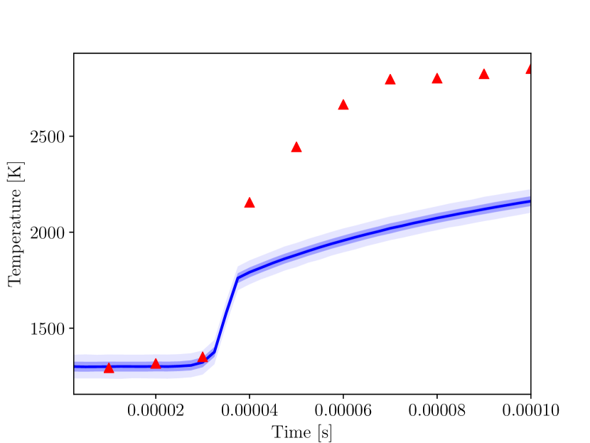
(a)

Figure 2: Concentrations and temperature time-series, $\phi=1.0$, $T_{0}=$1300\text{\,}\mathrm{K}$$. Observations (red triangles), reduced model $\mathcal{R}$ (blue curves), plotted with $65$ and $95\%$ confidence intervals.

5.3 Formulation of the inadequacy operator $\mathcal{S}$

The elements in the reduced model are H and O. Thus, the catchall species for the inadequacy operator are H^′ and O^′. Thus, the state for the enriched model is

$$\bm{x}^{S}=[x_{1},x_{2},\dots,x_{9}]^{T},$$

with the concentrations given in the order of H^′, O^′, H₂, O₂, H, O, OH, HO₂, H₂O. Note that $m_{R}=5$, $n_{R}=7$, $n_{\alpha}=2$, $n_{S}=9$.

5.3.1 The random matrix $S$

From theorem 3.1, we know that the matrix has the following structure:

$$S=\begin{pmatrix}s_{1,1}&0&s_{1,3}&0&s_{1,5}&0&s_{1,7}&s_{1,8}&s_{1,9}\\ 0&s_{2,2}&0&s_{2,4}&0&s_{2,6}&s_{2,7}&s_{2,8}&s_{2,9}\\ s_{3,1}&0&s_{3,3}&0&s_{3,5}&0&s_{3,7}&s_{3,8}&s_{3,9}\\ 0&s_{4,2}&0&s_{4,4}&0&s_{4,6}&s_{4,7}&s_{4,8}&s_{4,9}\\ s_{5,1}&0&s_{5,3}&0&s_{5,5}&0&s_{5,7}&s_{5,8}&s_{5,9}\\ 0&s_{6,2}&0&s_{6,4}&0&s_{6,6}&s_{6,7}&s_{6,8}&s_{6,9}\\ 0&0&0&0&0&0&s_{7,7}&s_{7,8}&s_{7,9}\\ 0&0&0&0&0&0&s_{8,7}&s_{8,8}&s_{8,9}\\ 0&0&0&0&0&0&s_{9,7}&s_{9,8}&s_{9,9}\\ \end{pmatrix}.$$

Here, of the 81 entries of $S$, 42 are identically zero. Next $E$ is the $n_{\alpha}\times n_{S}$ matrix:

$$E=\begin{pmatrix}1&0&1&0&1&0&1/2&1/3&2/3\\ 0&1&0&1&0&1&1/2&2/3&1/3\end{pmatrix}.$$

The first row of $E$ corresponds to hydrogen atoms and the second to oxygen. $C$ is the following $n_{S}\times n_{R}$ matrix whose columns span $\text{null}(E)$:

$$C=\begin{pmatrix}-1&0&-1&0&-1/2&-1/3&-2/3\\ 0&-1&0&-1&-1/2&-2/3&-1/3\\ 1&0&0&0&0&0&0\\ 0&1&0&0&0&0&0\\ 0&0&1&0&0&0&0\\ 0&0&0&1&0&0&0\\ 0&0&0&0&1&0&0\\ 0&0&0&0&0&1&0\\ 0&0&0&0&0&0&1\end{pmatrix}.$$

$P$ is an $n_{R}\times n_{S}$ matrix, where $S=CP$:

$$P=\begin{pmatrix}p_{1,1}&0&p_{1,3}&0&p_{1,5}&0&p_{1,7}&p_{1,8}&p_{1,9}\\ 0&p_{2,2}&0&p_{2,4}&0&p_{2,6}&p_{2,7}&p_{2,8}&p_{2,9}\\ p_{3,1}&0&p_{3,3}&0&p_{3,5}&0&p_{3,7}&p_{3,8}&p_{3,9}\\ 0&p_{4,2}&0&p_{4,4}&0&p_{4,6}&p_{4,7}&p_{4,8}&p_{4,9}\\ 0&0&0&0&0&0&p_{5,7}&p_{5,8}&p_{5,9}\\ 0&0&0&0&0&0&p_{6,7}&p_{6,8}&p_{6,9}\\ 0&0&0&0&0&0&p_{7,7}&p_{7,8}&p_{7,9}\end{pmatrix}.$$

The transformation from the entries of $P$ to $\bm{\xi}$ is given in table C.1, and the constraints are now

$$\xi_{i}\geq 0,\quad i=1,\dots,33.$$

Finally, to complete the formulation of $S$,

$$\xi_{i}\sim\log\mathcal{N}(\mu^{\xi}_{i},\eta^{\xi}_{i}),\quad i=1,\dots,33.$$

5.3.2 The catchall reactions $\mathcal{A}$

The catchall reactions allow the catchall species to directly form any species made up of more than one type of atom. Otherwise, that reaction is already allowed via $S$ ($\cee{H$^{\prime}$->H}$ is allowed by $S$ for example). Thus, there are three catchall reactions: Figure 3: Concentrations and temperature time-series, $\phi=0.9$, $T_{0}=$1200\text{\,}\mathrm{K}$$. Observations (red triangles), reduced model enriched with stochastic operator inadequacy representation $\mathcal{O}$ (blue curves), plotted with $65$ and $95\%$ confidence intervals.

Figure 4: Concentrations and temperature time-series, $\phi=1.0$, $T_{0}=$1300\text{\,}\mathrm{K}$$. Observations (red triangles), reduced model enriched with stochastic operator inadequacy representation $\mathcal{O}$ (blue curves), plotted with $65$ and $95\%$ confidence intervals.

Figure 5: Concentrations and temperature time-series, $\phi=1.1$, $T_{0}=$1400\text{\,}\mathrm{K}$$. Observations (red triangles), reduced model enriched with stochastic operator inadequacy representation $\mathcal{O}$ (blue curves), plotted with $65$ and $95\%$ confidence intervals.

5.5 Prediction

We conclude this section by predicting the concentrations and temperature for an extrapolative scenario—i.e., an initial condition outside the range of those used to generate calibration data. The stochastic operator approach developed in this work has been specifically designed with this use in mind, and it is formulated such that there is the potential, with appropriate validation tests, that such an extrapolative prediction could be supported by available information. While there are still possible improvements to the formulation, including the temperature dependence discussed in §LABEL:sec:ex_step56 and other possible extensions mentioned in §6, the fact that a validated extrapolative prediction is a possibility distinguishes this formulations from most other inadequacy representations. Indeed, to the authors’ knowledge, this is the only existing model inadequacy formulation for chemistry that has the potential to make a validated prediction outside of the range of the calibration data.

The prediction scenario shown here is a higher equivalence ratio and lower initial temperature than included in the calibration data set. Specifically, the initial condition is given by $\phi=1.15$ and $T_{0}=$1150\text{\,}\mathrm{K}$$. Although the corresponding output from the detailed model was not used to calibrate the model, the detailed model output is shown analogously to the previous results. Since the detailed model data are available, this extrapolation case can be viewed as an additional validation test of the calibrated stochastic operator model.

For completeness of the exercise, the reduced model output for the same prediction scenario is shown first in figure 5.5. As expected based on the calibration results, the reduced model alone is entirely incapable of capturing the behavior of the system, and many of the points from the detailed model fall outside the $65$ and $95\%$ confidence intervals predicted by the reduced model.

Figure 6: Predicted concentrations and temperature time-series, $\phi=1.15$, $T_{0}=$1150\text{\,}\mathrm{K}$$. Observations (red triangles), reduced model (blue curves), plotted with $65$ and $95\%$ confidence intervals.

Figure 5.5 shows results from the stochastic operator model. Unlike the reduced model alone, for the enriched model with the stochastic operator, all observations are consistent with the prediction, with $\gamma$ values all greater than 0.01.

Figure 7: Predicted concentrations and temperature time-series, $\phi=1.15$, $T_{0}=$1150\text{\,}\mathrm{K}$$. Observations (red triangles), reduced model enriched with stochastic operator inadequacy representation $\mathcal{O}$ (blue curves), plotted with $65$ and $95\%$ confidence intervals.

6 Conclusion

This study addresses the critical problem of model inadequacy that affects nearly all mathematical models of physical systems. In particular, we develop a novel approach to representing model inadequacy in chemical kinetics models. The approach relies on a stochastic operator that combines the flexibility and generality of a probabilistic model with the available deterministic physical information. In the context of predictive models, these two properties are essential, ensuring that the model is flexible enough to adapt to fit available observations without generating non-physical behavior.

The stochastic operator $\mathcal{S}$ contains three main components: 1) the random matrix $S$, 2) the nonlinear catchall reactions $\mathcal{A}$, and 3) the energy operator $\mathcal{W}$. The random matrix $S$ contains most of the information in $\mathcal{S}$ and has some interesting properties. Typically, the matrix has many identically zero entries. It always has a negative diagonal, is diagonally dominant, and has non-positive eigenvalues. The reactions in $\mathcal{A}$ allow any species in the reduced model to be the chemical product of the corresponding catchall species (if this is not already possible through $S$). Both $S$ and $\mathcal{A}$ guarantee conservation of atoms and non-negativity of concentrations. Finally, the energy operator $\mathcal{W}$ modifies the time derivative of temperature by endowing the catchall species with internal energy.

The inadequacy operator is tested on an example H₂/O₂ mechanism. Starting with a reduced mechanism that was shown to be invalid for prediction, the stochastic operator model is able to account for the model inadequacy. The observations used for calibration are plausible outcomes of the operator model—i.e., the concentrations and temperature values from the operator model $\mathcal{O}$ are consistent with the data supplied by the detailed model $\mathcal{D}$. Moreover, the prediction case showed that the operator model output was consistent with all of the observations from the detailed model for a scenario outside the range of initial conditions used for the operator calibration.

There are many avenues for extending the work reported here. Ongoing research includes the application of the operator to a more complex chemical setting, namely, a methane-air mechanism. We are also investigating a more complex physical setting with a more complex prediction problem: the prediction of a hydrogen laminar flame using the calibrated operator found in this work. Consistent with the discussion in §LABEL:sec:ex_step56, preliminary research on these topics has suggested that the temperature-independence of the operator (save $\mathcal{W}$) is too severe a limitation, and that in complex problems, the more information incorporated into the stochastic operator, the better. Thus, immediate goals are to include more physical information in the inadequacy representation such as realistic temperature-dependence, and to use stronger priors based on knowledge of the chemical reactions and the physical setup. This leads to the next major opportunity for future work: developing the connection between the stochastic operator and the actual chemistry. Mapping between the random matrix and the typical chemical reactions was a first step in this direction. However, a better understanding of what the stochastic operator means in physical terms is needed. This includes not just the structure, but also the uncertainty in the calibrated parameters. A future goal is to infer something about the missing chemistry from the calibrated operator. This is important when developing mechanisms based on experimental data, when no detailed mechanism is available.

Further, it is unclear that the random matrix coupled with catchall species and reactions is the optimal way to formulate the stochastic operator. The inadequacy formulation introduces many calibration parameters, which in turn increase the computational complexity. While the increase in dimensionality was manageable in this example problem, it may become impractical in more complex problems, especially when the reduced kinetics model is more complex. A number of alternative formulations are being pursued. For example, instead of using the random matrix $S$ and the catchall reactions in $\mathcal{A}$, a simplified version is the following: given $n_{R}$ species in the reduced model, include $n_{R}$ reversible dissociation reactions where the reactant is one of the original species and the products are the corresponding catchall species. In the reverse combination reaction, the catchall atoms react to form any of the original species. In this fashion, the atoms of any species could move to any other species in two steps. This representation would lose the flexibility possible in the current formulation; that is, the current formulation allows for the most detailed and direct linear movement from one species to another. If any such direct pathway proves significant, this would not be captured by this simplified formulation. On the other hand, it would decrease the number of random variables and thus would be more tractable in more complex reaction systems. With a smaller number of additional reactions, the corresponding reaction rates could then be enriched with temperature-dependence.

Another variation could be a more complete set of nonlinear reactions. Instead of only allowing the nonlinear catchall reactions, one could augment the reduced model with all or some subset of all possible nonlinear terms. In contrast to the first variation, this would increase the number of random variables. A formulation like this might only be possible with more informative priors or knowledge about the chemical system.

Finally, it would be very informative to apply this method to new problems. For instance, the inadequacy operator could be tested by a more realistic combustion problem. It may be that doing so requires a more complete thermodynamic description of the catchall species. More importantly, there is no reason to restrict the stochastic operator approach developed here to models of chemically reacting gas mixtures. Similar model structures and inadequacies appear in many other modeling domains. The guiding principles of this work (respecting physical constraints, maintaining flexibility, starting with a linearized version) and developing an analogous operator (possibly random matrix) should be explored in many different physical settings. Applications in many different domains could bring to light new challenges and common strengths for the stochastic operator approach to representing model inadequacy.

Appendix A Reaction mechanisms

The 21 reactions in the detailed hydrogen-oxygen mechanism are listed in table A and the five of the reduced mechanism in A. The associated reaction rate is $k=AT^{b}e^{-E/R^{\circ}T}$.

Units: mol, cm, s, kJ, K.

Table A.1: The detailed H₂/O₂ reaction mechanism from [62].

Units: mol, cm, s, kJ, K.

Table A.2: The reduced H₂/O₂ reaction mechanism from [62].

Appendix B Properties of $S$

B.1 Sparsity

As noted in §3.2.3, $S$ is often sparse. There is a way to determine which entries of $S$ are identically zero using the physical restrictions about how different species concentrations interact with each other. To determine the sparsity in this way, each species $\mathbb{X}$ is characterized by a composite number $\rho_{\mathbb{X}}$. First associate a prime number $p_{i}$ with each atom type $i=1,\dots n_{\alpha}$. Each species $\mathbb{X}$ is made up of a collection of atom types; let $\rho_{\mathbb{X}}$ be the product of prime numbers corresponding to each type of atom making up species $\mathbb{X}$. For example, if elements H and O correspond to the prime numbers 2 and 3, then $\rho_{\text{H}}=2$ and $\rho_{\text{H}_{2}\text{O}}=6$. In effect, this yields a prime number representation of each species where multiplicity is ignored.

Next, the columns of $S$ correspond to chemical reactants and the rows to chemical products. The entry $s_{ij}$ controls how many atoms move from species $j$—a sort of reactant—to species $i$—a sort of product. The operator can only move a positive amount of species $\mathbb{X}_{j}$ to $\mathbb{X}_{i}$ if the former contains all elements that comprise the latter. If not, then the $\text{gcd}(\rho_{\mathbb{X}_{i}},\rho_{\mathbb{X}_{j}})<\rho_{\mathbb{X}_{i}}$. But in this case there can be no flow of atoms from $\mathbb{X}_{j}$ to $\mathbb{X}_{i}$, and thus $s_{ij}\equiv 0$.

This technique can also be used to count the total number of entries that are identically zero in the matrix. Call this total number $\Omega$ and, for $i=1,\dots,n_{S}$, let $\lambda_{i}$ be the number of species $\mathbb{X}_{j}$ such that $\gcd(\rho_{\mathbb{X}_{i}},\rho_{\mathbb{X}_{j}})<\rho_{\mathbb{X}_{i}}$. By the argument in the previous paragraph, $\lambda_{i}$ is the number of zeros in the $i$th column of $S$. Then the number of zeros in $S$ is $\Omega=\sum_{i=1}^{n_{S}}\lambda_{i}$ because the sum is taken with respect to the different species, and each of these correspond to a different column of $S$.

B.2 Non-positivity of eigenvalues

Enforcing the two constraints— (I) conservation of atoms and (II) non-negativity of concentrations yields some interesting properties of the random matrix $S$. The non-positivity of eigenvalues is consistent with the constraints: no species can grow arbitrarily large over time. The proof follows:

Theorem B.1.

Let $S$ be any random matrix such that $ES=0$ and the off-diagonal elements of $S$ be non-negative. Then (a) the columns sum to zero, (b) the diagonal is negative, (c) the matrix is weakly diagonally dominant, and (d) the eigenvalues are non-positive.

Proof B.2.

(a) Consider $ES_{(\cdot,j)}=0$, where $S_{(\cdot,j)}$ is the $j$th column of $S$. There are $n_{\alpha}$ equations:

$$e_{1,1}s_{1,j}+e_{1,2}s_{2,j}+\dots+e_{1,n_{S}}s_{n_{S},j} =0$$

$$e_{2,1}s_{1,j}+e_{2,2}s_{2,j}+\dots+e_{2,n_{S}}s_{n_{S},j} =0$$

$$\vdots$$

$$e_{n_{\alpha},1}s_{1,j}+e_{n_{\alpha},2}s_{2,j}+\dots+e_{n_{\alpha},n_{P}}s_{n_{S},j} =0.$$

Now add the lines together:

(36) $$\sum_{i}{\sum_{k}{e_{k,i}}s_{i,j}}=0,$$

but $\sum_{k}{e_{k,i}}=1$ by definition. Thus,

(b) In equation (LABEL:eq:colsum), move the diagonal term to the RHS:

(38) $$\sum_{i\neq j}s_{i,j}=-s_{j,j}.$$

Since all off-diagonal terms are non-negative, it must be that the diagonal element is negative.

(c) The line above also shows weak diagonal dominance, since

(39) $$|s_{j,j}| =\left|\sum_{i\neq j}s_{i,j}\right|$$

(40) $$=\sum_{i\neq j}|s_{i,j}|,$$

where the second equality holds because all off-diagonal elements are non-negative.

(d) Since $S$ and $S^{T}$ have the same eigenvalues, we will show that the claim is true for $S^{T}$. Let $B=S^{T}$ and $B_{i}=\sum_{j\neq i}|b_{i,j}|=\sum_{j\neq i}b_{i,j}$ be the sum of off-diagonals in the $i$th row. Now let $D(b_{i,i},B_{i})$ be the closed disc centered at $b_{i,i}$ with radius $B_{i}$. Then the Gershgorin theorem states that every eigenvalue of $B$ lies within at least one of the discs [6]. In this case, we have $b_{i,i}=s_{i,i}$ and $B_{i}=|s_{i,i}|$, so every eigenvalue lies within at least one disc $D(s_{i,i},|s_{i,i}|)$, where $s_{i,i}\leq 0$.

Appendix C Transform from $\bm{p}$ to $\bm{\xi}$

$\xi_{i}$ =	$p_{j,k}$
$\xi_{1}$ =	$p_{1,1}$
$\xi_{2}$ =	$-(p_{1,3}+p_{3,3})$
$\xi_{3}$ =	$p_{1,5}$
$\xi_{4}$ =	$p_{1,7}$
$\xi_{5}$ =	$p_{1,8}$
$\xi_{6}$ =	$p_{1,9}$
$\xi_{7}$ =	$p_{2,2}$
$\xi_{8}$ =	$-(p_{2,4}+p_{4,4})$
$\xi_{9}$ =	$p_{2,6}$
$\xi_{10}$ =	$p_{2,7}$
$\xi_{11}$ =	$p_{2,8}$
$\xi_{12}$ =	$p_{2,9}$
$\xi_{13}$ =	$p_{3,1}$
$\xi_{14}$ =	$p_{3,3}$
$\xi_{15}$ =	$-(p_{3,5}+p_{1,5})$
$\xi_{16}$ =	$p_{3,7}$
$\xi_{17}$ =	$p_{3,8}$
$\xi_{18}$ =	$p_{3,9}$
$\xi_{19}$ =	$p_{4,2}$
$\xi_{20}$ =	$p_{4,4}$
$\xi_{21}$ =	$-(p_{4,6}+p_{2,6})$
$\xi_{22}$ =	$p_{4,7}$
$\xi_{23}$ =	$p_{4,8}$
$\xi_{24}$ =	$p_{4,9}$
$\xi_{25}$ =	$-p_{5,7}-2(p_{1,7}+p_{2,7}+p_{3,7}+p_{4,7}+(2/3)p_{6,7}+(2/3)p_{7,7})$
$\xi_{26}$ =	$p_{5,8}$
$\xi_{27}$ =	$p_{5,9}$
$\xi_{28}$ =	$p_{6,7}$
$\xi_{29}$ =	$-p_{6,8}-3(p_{1,8}+p_{2,8}+p_{3,8}+p_{4,8}+(1/2)p_{5,8}+(2/3)p_{7,8})$
$\xi_{30}$ =	$p_{6,9}$
$\xi_{31}$ =	$p_{7,7}$
$\xi_{32}$ =	$p_{7,8}$
$\xi_{33}$ =	$-p_{7,9}-3(p_{1,9}+p_{2,9}+p_{3,9}+p_{4,9}+(1/2)p_{5,9}+(2/3)p_{6,9})$

Table C.1: The transformed variables $\bm{\xi}$ for the H₂/O₂ operator.

References

- [1] A New Templated Implementation of Chemistry Hydrodynamics (Antioch). https://github.com/libantioch/antioch.
- [2] MIT Uncertainty Quantification Library (MUQ). https://bitbucket.org/mituq/muq.
- [3] I. Babuska, F. Nobile, and R. Tempone. A systematic approach to model validation based on Bayesian updates and prediction related rejection criteria. Computer Methods in Applied Mechanics and Engineering, 197:2517–2539, May 2008.
- [4] G. R. Barth, M. C. Hill, T. H. Illangasekare, and H. Rajaram. Predictive modeling of flow and transport in a two-dimensional intermediate-scale, heterogeneous porous medium. Water Resources Research, 37(10):2503–2512, 2001.
- [5] M. J. Bayarri, J. O. Berger, R. Paulo, J. Sacks, J. A. Cafeo, J. Cavendish, C.-H. Lin, and J. Tu. A framework for validation of computer models. Technometrics, 49(2):138–154, May 2007.
- [6] H. E. Bell. Gershgorin’s theorem and the zeros of polynomials. American Mathematical Monthly, 72:292–295, 1965.
- [7] M. L. Berliner. Hierarchical Bayesian time series models. In K. M. Hanson and R. N. Silver, editors, Maximum Entropy and Bayesian Methods, volume 79 of Fundamental Theories of Physics, pages 15–22. Springer Netherlands, 1996.
- [8] C. E. Bonferroni. Il calcolo delle assicurazioni su gruppi di teste. In Studi in Onore del Professore Salvatore Ortu Carboni, pages 13–60. Rome, 1935.
- [9] G. E. P. Box and G. C. Tiao. Bayesian Inference in Statistical Analysis. Wiley-Interscience, 1 edition, Apr. 1992.
- [10] K. Braman, T. A. Oliver, and V. Raman. Bayesian analysis of syngas chemistry models. Combustion Theory and Modelling, 17(5):858–887, 2013.
- [11] M. P. Burke, M. Chaos, Y. Ju, F. L. Dryer, and S. J. Klippenstein. Comprehensive H2/O2 kinetic model for high-pressure combustion. International Journal of Chemical Kinetics, 44(7):444–474, Dec. 2011.
- [12] M. P. Burke, M. Chaos, Y. Ju, F. L. Dryer, and S. J. Klippenstein. Comprehensive H2/O2 kinetic model for high-pressure combustion. International Journal of Chemical Kinetics, 44(7):444–474, July 2012.
- [13] D. Calvetti and E. Somersalo. An Introduction to Bayesian Scientific Computing: Ten Lectures on Subjective Computing, 2007.
- [14] Center for Predictive Engineering and Computational Sciences. Quantification of Uncertainty for Estimation, Simulation, and Optimization (QUESO) User’s Manual, 2013.
- [15] S. H. Cheung, T. A. Oliver, E. E. Prudencio, S. Prudhomme, and R. D. Moser. Bayesian uncertainty analysis with applications to turbulence modeling. Reliability. Eng. System Safety, 96:1137–1149, 2011.
- [16] R. P. Christian. The Bayesian Choice. Springer, 2001.
- [17] Conaire, H. J. Curran, J. M. Simmie, W. J. Pitz, and C. K. Westbrook. A comprehensive modeling study of hydrogen oxidation. International Journal of Chemical Kinetics, 36(11):603–622, Nov. 2004.
- [18] M. K. Cowles and B. P. Carlin. Markov chain Monte Carlo convergence diagnostics: A comparative review. American Statistical Association, 91(434):883–904, June 1996.
- [19] R. T. Cox. The Algebra of Probable Inference. Johns Hopkins University Press, 1961.
- [20] M. H. DeGroot and M. J. Schervish. Probability and Statistics (4th Edition). Pearson, 4 edition, Jan. 2011.
- [21] A. Edelman and N. R. Rao. Random matrix theory. Acta Numerica, 14(-1):233–297, May 2005.
- [22] K. Farrell, J. T. Oden, and D. Faghihi. A bayesian framework for adaptive selection, calibration, and validation of coarse-grained models of atomistic systems. Journal of Computational Physics, 295:189–208, 2015.
- [23] M. Feinberg. Lectures on Chemical Reaction Networks. 1979.
- [24] A. Gelman. Exploratory Data Analysis for Complex Models. Journal of Computational and Graphical Statistics, 13(4):755–779, Dec. 2004.
- [25] A. Gelman, X.-l. Meng, and H. Stern. Posterior predictive assessment of model fitness via realized discrepancies. In Statistica Sinica, pages 733–807, 1996.
- [26] W. R. Gilks, S. Richardson, and D. Spiegelhalter. Markov Chain Monte Carlo in Practice. Chapman and Hall/CRC, softcover reprint of the original 1st ed. 1996 edition, Dec. 1996.
- [27] D. T. Gillespie. Stochastic simulation of chemical kinetics. Annual Review of Physical Chemistry, 58:35–55, 2007.
- [28] H. Haario, M. Laine, A. Mira, and E. Saksman. DRAM: Efficient adaptive MCMC. Statistics and Computing, 16(4):339–354, Dec. 2006.
- [29] D. Higdon, J. Gattiker, B. Williams, and M. Rightley. Computer model calibration using high-dimensional output. Journal of the American Statistical Association, 103(482):570–583, June 2008.
- [30] D. Higdon, M. Kennedy, J. C. Cavendish, J. A. Cafeo, and R. D. Ryne. Combining field data and computer simulations for calibration and prediction. SIAM Journal on Scientific Computing, 26(2):448–466, Jan. 2004.
- [31] E. T. Jaynes. Probability Theory: The Logic of Science. Cambridge University Press, 2003.
- [32] J. Kaipio and E. Somersalo. Statistical and Computational Inverse Problems. Springer, 2005.
- [33] G. Karlebach and R. Shamir. Modelling and analysis of gene regulatory networks. Nature Reviews Molecular Cell Biology, 9(10):770–780, 2008.
- [34] M. C. Kennedy and A. O’Hagan. Bayesian calibration of computer models. Journal of the Royal Statistical Society: Series B (Statistical Methodology), 63(3):425–464, Jan. 2001.
- [35] A. A. Konnov. Remaining uncertainties in the kinetic mechanism of hydrogen combustion. Combustion and Flame, 152(4):507–528, Mar. 2008.
- [36] D. Lunn, A. Thomas, N. Best, and D. Spiegelhalter. WinBUGS - A Bayesian modelling framework: Concepts, structure, and extensibility. 10(4):325–337, 2000.
- [37] B. J. McBride, S. Gordon, and M. A. Reno. NASA Technical Memorandum 4513: Coefficients for Calculating Thermodynamic and Transport Properties of Individual Species. Technical report, National Aeronautics and Space Administration, 1993.
- [38] M. L. Mehta. Random Matrices, Volume 142, Third Edition (Pure and Applied Mathematics). Academic Press, 3 edition, Nov. 2004.
- [39] K. Miki, S. H. Cheung, E. E. Prudencio, and P. L. Varghese. Bayesian uncertainty quantification of recent shock tube determinations of the rate coefficient of reaction H + O2→ OH + O. International Journal of Chemical Kinetics, 44(9):586–597, July 2012.
- [40] R. G. Miller. Simultaneous Statistical Inference (Springer Series in Statistics). Springer, 2nd edition, Mar. 1981.
- [41] R. D. Moser and T. A. Oliver. Validation of physical models in the precense of uncertainty. In R. Ghanem, D. Higdon, and H. Owhadi, editors, Handbook of Uncertainty Quantification. Springer, 2016.
- [42] M. A. Mueller, T. J. Kim, R. A. Yetter, and F. L. Dryer. Flow reactor studies and kinetic modeling of the H2/O2 reaction. Int. J. Chem. Kinet., 31(2):113–125, Jan. 1999.
- [43] W. L. Oberkampf, T. G. Trucano, and C. Hirsch. Verification, validation, and predictive capability in computational engineering and physics. Applied Mechanics Reviews, 57(5):345–384, 2004.
- [44] J. T. Oden, T. Belytschko, J. Fish, T. Hughes, C. Johnson, D. Keyes, A. Laub, L. Petzold, D. Srolovitz, and S. Yip. Revolutionizing engineering science through simulation. National Science Foundation Blue Ribbon Panel Report, 65, 2006.
- [45] T. A. Oliver and R. D. Moser. Accounting for uncertainty in the analysis of overlap layer mean velocity models. Phys. of Fluids, 24:075108, 2012.
- [46] T. A. Oliver, G. Terejanu, C. S. Simmons, and R. D. Moser. Validating predictions of unobserved quantities. Computational Methods in Applied Mechanics and Engineering, 283:1310–1335, 2015.
- [47] E. Prudencio and S. H. Cheung. Parallel adaptive multilevel sampling algorithms for the Bayesian analysis of mathematical models. International Journal for Uncertainty Quantification, 2(3):215–237, 2012.
- [48] D. B. Rubin. More powerful randomization-based p-values in double-blind trials with non-compliance. Statist. Med., 17(3):371–385, Feb. 1998.
- [49] S. Sankararaman, Y. Ling, and S. Mahadevan. Uncertainty quantification and model validation of fatigue crack growth prediction. Engineering Fracture Mechanics, 78(7):1487–1504, 2011.
- [50] K. Sargsyan, H. Najm, and R. Ghanem. On the statistical calibration of physical models. International Journal of Chemical Kinetics, 47(4):246–276, 2015.
- [51] D. E. Schiavazzi, A. Baretta, G. Pennati, T.-Y. Hsia, and A. L. Marsden. Patient-specific parameter estimation in single-ventricle lumped circulation models under uncertainty. International journal for numerical methods in biomedical engineering, 33(3), 2017.
- [52] L. E. Schwer. Guide for verification and validation in computational solid mechanics. 2009.
- [53] D. S. Sivia and J. Skilling. Data Analysis: A Bayesian Tutorial. Oxford University Press, 2006.
- [54] G. P. Smith, D. M. Golden, M. Frenklach, N. W. Moriarty, B. Eiteneer, M. Goldenberg, C. T. Bowman, R. K. Hanson, S. Song, W. C. Gardiner, V. V. Lissianski, and Q. Zhiwei. GRI-Mech. http://www.me.berkeley.edu/gri_mech/. Accessed: 2015-01-15.
- [55] C. Soize. Random matrix theory for modeling uncertainties in computational mechanics. Computer Methods in Applied Mechanics and Engineering, 194(12-16):1333–1366, Apr. 2005.
- [56] C. Soize. Generalized probabilistic approach of uncertainties in computational dynamics using random matrices and polynomial chaos decompositions. Int. J. Numer. Meth. Engng., 81(8):939–970, Feb. 2010.
- [57] J. I. Steinfeld, J. S. Francisco, and W. L. Hase. Chemical Kinetics and Dynamics. Prentice Hall, 1998.
- [58] L. P. Swiler. Gaussian processes in response surface modeling. Society of Experimental Mechanics Meeting, Jan. 2006.
- [59] P. R. Westmoreland. Reduced kinetic mechanisms for applications in combustion systems. Edited by N. Peters and B. Rogg, Spring-Verlag, New York, Lecture Notes in Physics, Monograph 15, 1993, 360 pp. AIChE J., 40(11):1926–1927, Nov. 1994.
- [60] C. K. Wikle, R. F. Milliff, D. Nychka, and L. M. Berliner. Spatiotemporal hierarchical Bayesian modeling: Tropical ocean surface winds. Journal of the American Statistical Association, 96(454):382–397, June 2001.
- [61] F. A. Williams. Combustion Theory: Second Edition (Combustion Science and Engineering). Westview Press, second edition edition, Mar. 1994.
- [62] F. A. Williams. Detailed and reduced chemistry for hydrogen autoignition. Journal of Loss Prevention in the Process Industries, 21(2):131–135, Mar. 2008.