Robust 3D Localization and Tracking of Sound Sources Using Beamforming and Particle Filtering

Abstract

In this paper we present a new robust sound source localization and tracking method using an array of eight microphones (US patent pending) . The method uses a steered beamformer based on the reliability-weighted phase transform (RWPHAT) along with a particle filter-based tracking algorithm. The proposed system is able to estimate both the direction and the distance of the sources. In a videoconferencing context, the direction was estimated with an accuracy better than one degree while the distance was accurate within 10% RMS. Tracking of up to three simultaneous moving speakers is demonstrated in a noisy environment.

1 Introduction

Sound source localization is defined as the determination of the coordinates of sound sources in relation to a point in space. This can be very useful in videoconference application, either for directing the camera toward the person speaking, or as an input to a sound source separation algorithm [1] to improve sound quality. Sound source tracking has been demonstrated before by using Kalman filtering [2] and particle filtering [3]. However, this has only been experimentally demonstrated with a single sound source at a time. Our work demonstrates that it is possible to track multiple sound sources using particle filters by solving the source-observation assignment problem.

The proposed sound localization and tracking system is composed of two parts: a microphone array, a memoryless localization algorithm based on a steered beamformer, and a particle filtering tracker. The steered beamformer is implemented in the frequency domain and scans the space for energy peaks. The robustness of the steered beamformer is enhanced by the use of the reliability weighted phase transform (RWPHAT). The result of the first localization is then processed by a particle filter that tracks each source while also preventing false detections.

This approach improves on an earlier work in mobile robotics [4] and can estimate not only the direction, but the distance of sound sources. Localization accuracy and tracking capabilities of the system are reported in a videoconferencing context. In that application, the ability to estimate the source distance is significant as it solves the parallax problem for the case when the camera is not located at the center of the microphone array. We use a circular array because it is the most convenient shape for our videoconferencing application.

The paper is organized as follows. Section 2 describes our steered beamformer based on the RWPHAT. Section 3 explains how tracking is performed using a particle filter. This is followed by experimental results and a discussion in Section 4. Section 5 concludes the paper and presents future work.

2 Beamformer-Based Sound Localization

The basic idea behind the steered beamformer approach to source localization is to steer a beamformer in all possible locations and look for maximal output. This can be done by maximizing the output energy of a simple delay-and-sum beamformer.

2.1 Reliability-Weighted Phase Transform

It was shown in [4] that the output energy of an $M$-microphone delay-and-sum beamformer can be computed as a sum of microphone pair cross-correlations $R_{x_{m_{1}},x_{m_{2}}}\left(\tau_{m_{1}}-\tau_{m_{2}}\right)$, plus a constant microphone energy term $K$:

$$E=K+2\sum_{m_{1}=0}^{M-1}\sum_{m_{2}=0}^{m_{1}-1}R_{x_{m_{1}},x_{m_{2}}}\left(\tau_{m_{1}}-\tau_{m_{2}}\right)$$ (1)

where $x_{m}\left(n\right)$ is the signal from the $m^{th}$ microphone and $\tau_{m}$ is the delay of arrival (in samples) for that microphone. Assuming that only one sound source is present, we can see that $E$ will be maximal when the delays $\tau_{m}$ are such that the microphone signals are in phase, and therefore add constructively.

The cross-correlation function can be approximated in the frequency domain. A popular variation on the cross-correlation is the phase transform (PHAT). Some of its advantages include sharper cross-correlation peaks and a certain level of robustness to reverberation. However, its main drawback is that all frequency bins of the spectrum have the contribution to the final correlation, even if the signal at some frequencies is dominated by noise or reverberation. As an improvement over the PHAT, we introduce the reliability-weighted phase transform (RWPHAT) defined as:

$$R_{i,j}^{RWPHAT}(\tau)=\sum_{k=0}^{L-1}\frac{\zeta_{i}(k)X_{i}(k)\zeta_{j}(k)X_{j}(k)^{*}}{\left|X_{i}(k)\right|\left|X_{j}(k)\right|}e^{\jmath 2\pi k\tau/L}$$ (2)

where the weights $\zeta_{i}^{n}(k)$ reflect the reliability of each frequency component. It is defined as the Wiener filter gain:

$$\zeta_{i}^{n}(k)=\frac{\xi_{i}^{n}(k)}{\xi_{i}^{n}(k)+1}$$ (3)

where $\xi_{i}^{n}(k)$ is an estimate of the a priori SNR at the $i^{th}$ microphone, at time frame $n$, for frequency $k$, computed using the decision-directed approach proposed by Ephraim and Malah [5].

The noise term considered for the a priori SNR estimation is composed of a background noise term $\sigma_{i}^{2}(k)$ and a reverberation term $\lambda_{i}^{n}(k)$. Background noise is estimated using the Minima-Controlled Recursive Average (MCRA) technique [6], which adapts the noise estimate during periods of low energy. We use a simple exponential decay model for the reverberation:

$$\lambda_{i}^{n}(k)=\gamma\lambda_{i}^{n-1}(k)+(1-\gamma)\delta^{-1}\left|\zeta_{i}^{n}(k)X_{i}^{n-1}(k)\right|^{2}$$ (4)

where $\gamma$ is the reverberation decay (derived from the reverberation time) of the room, $\delta$ is the signal-to-reverberant ratio (SRR) and $R_{i}^{-1}(k)=0$. Equation 4 can be seen as modeling the precedence effect [7], ignoring frequency bins where a loud sound was recently present.

2.2 Search Procedure

Unlike previous work using spherical mesh composed of triangular [4], we now use a square grid folded onto a hemisphere. The square grid makes it easier to do refining steps and only a hemisphere is needed because of the ambiguity introduced by having all microphones in the same plane. For grid parameters $u$ and $v$ in the $[-1,1]$ range, the unit vector $\mathbf{u}$ defining the direction is expressed as:

$$\mathbf{u}=\left[\frac{v}{\sqrt{u^{2}+v^{2}}}\sin\phi,\>\frac{u}{\sqrt{u^{2}+v^{2}}}\sin\phi,\>\cos\phi\right]^{\mathrm{T}}$$ (5)

where $\phi=\pi\max\left(u^{2},v^{2}\right)/2$. The complete search grid is defined as the space covered by $d\mathbf{u}$, where $d$ is the distance to the center of the array.

The search for the location maximizing beamformer energy is performed using a coarse/fine strategy. Unlike work presented by [8], even the coarse search can proceed with a high resolution, with a 41x41 grid (4-degree interval) for direction and 5 possible distances. The fine search is then used to obtain an even more accurate estimation, with a 201x201 grid (0.9-degree interval) for direction and 25 possible distances ranging from 30 cm to 3 meters.

The cross-correlations $R_{i,j}^{RWPHAT}(\tau)$ are computed by averaging the cross-power spectra $X_{i}(k)X_{j}(k)^{*}$ over a time period of 4 frames (40 ms) for overlapping windows of 1024 samples at 48 kHz. Once the cross-correlations $R_{i,j}^{RWPHAT}\!(\tau)$ are computed, the search for the best location on the grid is performed using a lookup-and-sum algorithm where the time delay of arrival $\tau$ for each microphone pair and for each source location is obtained from a lookup table. For an array of 28 microphones, this means only 28 lookup-and-sum operations for each position searched, much less than would be required by a time-domain implementation. In the proposed configuration ($N=8405$, $M=8$), the lookup table for the coarse grid fits entirely in a modern processor’s L2 cache, so that the algorithm is not limited by memory access time.

After finding the loudest source by maximizing the energy of a steered beamformer, other sources can be localized by removing the contribution of the first source from the cross-correlations and repeating the process. In order to remove the contribution of a source, all values of $R_{i,j}^{RWPHAT}(\tau)$ that have been used in the sum that produced the maximal energy are reset to zero. The process is summarized in Algorithm 1. Since the beamformer does not know how many sources are present, it always looks for two sources. This situation leads to a high rate of false detection, even when two or more sources are present. That problem is handled by the particle filter described in the next section.

  for $q=1$ to assumed number of sources do

     for all grid index $k$ do

         $E_{k}\leftarrow\sum_{i,j}R^{RWPHAT}_{i,j}(lookup(k,i,j))$

     end for

     $D_{q}\leftarrow\textrm{argmax}_{k}\ (E_{k})$

     for all microphone pair $i,j$ do

         $R^{RWPHAT}_{i,j}(lookup(D_{q},i,j))\leftarrow 0$

     end for

  end for

Algorithm 1 Steered beamformer location search

3 Particle-Based Tracking

To remove false detection produced by the steered beamformer and track each sound source, we use a probabilistic temporal integration based on all measurements available up to the current time. It has been shown in [3, 9] that particle filters are an effective way of tracking sound sources. Using this approach, the pdf representing the location of each source is represented as a set of particles to which different weights (probabilities) are assigned. The choice of particle filtering over Kalman filtering is further justified by the non-gaussian probabilities arising from false detections and multiple sources.

At time $t$, we consider the case of $N_{s}$ sources ($j$ index) being tracked, each modeled using $N_{p}$ particles ($i$ index) of location $\mathbf{x}_{j,i}^{(t)}$ and weights $w_{j,i}^{(t)}$. The state vector for the particles is composed of six dimensions, three for position and three for its derivative:

$$\mathbf{s}_{j,i}^{(t)}=\left[\begin{array}[]{cc}\mathbf{x}_{j,i}^{(t)}&\mathbf{\dot{x}}_{j,i}^{(t)}\end{array}\right]^{\mathrm{T}}$$ (6)

We implement the sampling importance resampling (SIR) algorithm. The steps are described in the following subsections and generalize sound source tracking to an arbitrary and non-constant number of sources.

Prediction

As a predictor, we use the excitation-damping model as proposed in [3]:

$$\mathbf{\dot{x}}_{j,i}^{(t)} = a\mathbf{\dot{x}}_{j,i}^{(t-1)}+bF_{\mathbf{x}}$$ (7)

$$\mathbf{x}_{j,i}^{(t)} = \mathbf{x}_{j,i}^{(t-1)}+\Delta T\mathbf{\dot{x}}_{j,i}^{(t)}$$ (8)

where $a=e^{-\alpha\Delta T}$ controls the damping term, $b=\beta\sqrt{1-a^{2}}$ controls the excitation term, $F_{\mathbf{x}}$ is a Gaussian random variable of unit variance and $\Delta T$ is the time interval between updates.

Instantaneous Location Probabilities

The steered beamformer described in Section 2 produces an observation $O^{(t)}$ for each time $t$ that is composed of $Q$ potential source locations $\mathbf{y}_{q}$. We also denote $\mathbf{O}^{(t)}$, the set of all observations up to time $t$. We introduce the probability $P_{q}$ that the potential source $q$ is a true source (not a false detection) that can be interpreted as our confidence in the steered beamformer output. We know that the higher the beamformer energy, the more likely a potential source is to be true, so

$$P_{q}=\left\{\begin{array}[]{cc}\nu^{2}/2&\nu\leq 1\\ 1-\nu^{-2}/2,&\nu>1\end{array}\right.,\;\nu=E/E_{T}$$ (9)

where $E_{T}$ is the empirical threshold energy for 50% probability. Assuming that $\mathbf{y}_{q}$ is not a false detection, the probability density of observing $O_{q}^{(t)}$ for a source located at particle position $\mathbf{x}_{j,i}^{(t)}$ is given by a normal distribution centered at $\mathbf{x}_{j,i}$ with a standard deviation of 3 degrees for direction and a distance-dependent standard deviation for the distance.

Probabilities for Multiple Sources

Before we can derive the update rule for the particle weights $w_{j,i}^{(t)}$, we must first introduce the concept of source-observation assignment. For each potential source $q$ detected by the steered beamformer, we must compute $P_{q,j}$, the probability that the detection is caused by the tracked source $j$, $P_{q}(H_{0})$, the probability that the detection is a false alarm, and $P_{q}(H_{2})$, the probability that observation $q$ corresponds to a new source.

Fig. 1: Assignment example where one of the tracked sources is observed and one potential source is a false detection. The assignment can be described as $f(\{0,1\})=\{1,-2\}$.

Let $f:\{0,1,\ldots,Q-1\}\longrightarrow\{-2,-1,0,1,\ldots,M-1\}$ be a function assigning observations $q$ to the tracked sources $j$ (values -2 is used for false detection and -1 is used for a new source). Figure 1 illustrates a hypothetical case with the two potential sources detected by the steered beamformer and their assignment to the three tracked sources. Knowing $P\left(f\left|O^{(t)}\right.\right)$ (the probability that $f$ is the correct assignment given observation $O^{(t)}$) for all possible $f$, we can compute $P_{q,j}$ as the sum of the probabilities of all $f$ that assign potential source $q$ to tracked source $j$. The probabilities for new sources and false detections are obtained similarly.

Omitting $t$ for clarity, and assuming conditional independence of the observations given the mapping function, the probability $P(f|O)$ is given by:

$$P(f|O)=\frac{P(f)\prod_{q}p\left(\left.O_{q}\right|f(q)\right)}{p(O)}=\frac{P(f)\prod_{q}p\left(\left.O_{q}\right|f(q)\right)}{\sum_{f}P(f)\prod_{q}p\left(\left.O_{q}\right|f(q)\right)}$$ (10)

We assume that the distribution of the false detections ($H_{0}$) and the new sources ($H_{2}$) are uniform, while the distribution for tracked sources ($H_{1}$) is the pdf approximated by the particle distribution convolved with the steered beamformer error pdf:

$$p\left(\left.O_{q}\right|f(q)\right)=\sum_{i}w_{f(q),i}p\left(\left.O_{q}\right|\mathbf{x}_{j,i}\right)$$ (11)

The a priori probability of $f$ being the correct assignment is also assumed to come from independent individual components: $P(f)=\prod_{q}P\left(f(q)\right)$with:

$$P\left(f(q)\right)=\left\{\begin{array}[]{ll}\left(1-P_{q}\right)P_{false},&f(q)=-2\\ P_{q}P_{new}&f(q)=-1\\ P_{q}P\left(Obs_{j}^{(t)}\left|\mathbf{O}^{(t-1)}\right.\right)&f(q)\geq 0\end{array}\right.$$ (12)

where $P_{new}$ is the a priori probability that a new source appears and $P_{false}$ is the a priori probability of false detection and $P\left(Obs_{j}^{(t)}\left|\mathbf{O}^{(t-1)}\right.\!\right)\!=\!P\left(E_{j}\left|\mathbf{O}^{(t-1)}\right.\!\right)P\left(\mathrm{A}_{j}^{(t)}\left|\mathbf{O}^{(t-1)}\right.\!\right)$ is the probability that source $j$ is observable, i.e., that it exists ($E_{j}$) and it is active ($A_{j}^{(t)}$) at time $t$.

The probability that the source exists is computed using Bayes law over multiple time frames and considering the instantaneous probability of the source being observed $P_{j}^{(t-1)}$, as well as the a priori probability that the source exists despite not being observed. The probability that a source is active (non-zero signal) is computed by considering a first order Markov process with two states (active, inactive). The probability that an active source remains active is set to 0.95, and the probability that an inactive source becomes active again is set to 0.05. We assuming that the active and inactive states are a priori equiprobable.

Weight Update

At times $t$, assuming that the observations are conditionally independent given the source position, and knowing that for a given source $j$, $\sum_{i=1}^{N}w_{j,i}^{(t)}=1$, the new particle weights for source $j$ are defined as:

$$w_{j,i}^{(t)}=p\left(\mathbf{x}_{j,i}^{(t)}\left|\mathbf{O}^{(t)}\right.\right)=\frac{p\left(\mathbf{x}_{j,i}^{(t)}\left|O^{(t)}\right.\right)w_{j,i}^{(t-1)}}{\sum_{i=1}^{N}p\left(\mathbf{x}_{j,i}^{(t)}\left|O^{(t)}\right.\right)w_{j,i}^{(t-1)}}$$ (13)

The probability $p\left(\mathbf{x}_{j,i}^{(t)}\left|O^{(t)}\right.\right)$ is given by:

$$p\left(\mathbf{x}_{j,i}^{(t)}\left|O^{(t)}\right.\right)=\frac{\left(1-P_{j}^{(t)}\right)}{N}+P_{j}\frac{\sum_{q}P_{q,j}^{(t)}p\left(\left.O_{q}^{(t)}\right|\mathbf{x}_{j,i}^{(t)}\right)}{\sum_{i}\sum_{q}P_{q,j}^{(t)}p\left(\left.O_{q}^{(t)}\right|\mathbf{x}_{j,i}^{(t)}\right)}$$ (14)

Adding or Removing Sources

In a real environment, sources may appear or disappear at any moment. If, at any time, $P_{q}(H_{2})$ is higher than a threshold equal to $0.3$, we consider that a new source is present, in which case a set of particles is created for source $q$. Similarly, we set a time limit on sources so that if the source has not been observed for a certain amount of time, we consider that it no longer exists. In that case, the corresponding particle filter is no longer updated nor considered in future calculations.

Parameter Estimation

The estimated position of each source is the mean of the pdf and can be obtained as a weighted average of its particles position: $\bar{\mathbf{x}}_{j}^{(t)}=\sum_{i=1}^{N}w_{j,i}^{(t)}\mathbf{x}_{j,i}^{(t)}$

Resampling

Resampling is performed only when $N_{eff}\approx\left(\sum_{i=1}^{N}w_{j,i}^{2}\right)^{-1}<N_{min}$ [10]. That criterion ensures that resampling only occurs when new data is available for a certain source. Otherwise, this would cause unnecessary reduction in particle diversity, due to some particles randomly disappearing.

4 Results and Discussion

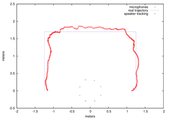
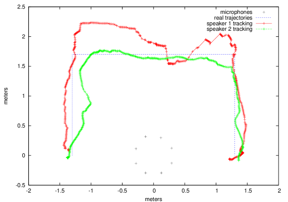
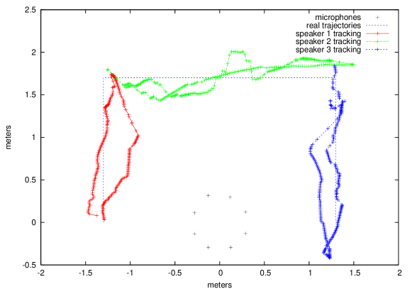
Fig. 2: Tracking results in the horizontal plane (time and elevation now shown). Left: one moving speaker (going from left to right), center: two moving speakers (speaker 1 going from right to left, speaker 2 going from left to right), right: three moving speakers going back and forth on each side.

The proposed localization system was tested using real recordings with a 60 cm circular array of eight omni-directional microphones resting on top of a table. The shape of the array is chosen for its symmetry and convenience in a videoconferencing setup, although the proposed algorithm would allow other positions. The testing environment is a noisy conference room resulting in an average SNR of 7 dB (assuming one speaker) and with moderate reverberation. Running the localization system in real-time required 30% of a 2.13 GHz Pentium-M CPU. For a stationary source at 1.5 meter distance, the angular accuracy was found to be better than one degree (below our measurement accuracy) while the distance estimate was found to have an RMS error of 10%. It is clear from these results that angular accuracy is much better than distance accuracy. This is a fundamental aspect that can be explained by the fact that distance only has a very small impact on the time delays perceived between the microphones.

Three tracking experiments were conducted. The results in Figure 2 show that the system is able to simultaneously track one, two or three moving sound sources. For the case of two moving sources, the particle filter is able to keep track of both sources even when they are crossing in front of the array. Because we lack the “ground truth” position for moving sources, only the distance error was computed (using the information about the height of the speakers) and found to be around 10% for all three experiments.

5 Conclusion

We have implemented a system that is able to localize and track simultaneous moving sound sources in the presence of noise and reverberation. The system uses an array of eight microphones and combines an RWPHAT-based steered beamformer with a particle filter tracking algorithm capable of following multiple sources.

An angular accuracy better than one degree was achieved with a distance measurement error of 10%, even for multiple moving speakers. To our knowledge, no other work has demonstrated tracking of direction and distance for multiple moving sound sources. The capability to track distance is important as it will allow a camera to follow a speaker even if it is not located at the center of the microphone array (parallax problem).

References

- [1] J.-M. Valin, J. Rouat, and F. Michaud, “Microphone array post-filter for separation of simultaneous non-stationary sources,” in Proc. ICASSP, 2004, pp. 221–224.
- [2] D. Bechler, M.S. Schlosser, and K. Kroschel, “System for robust 3D speaker tracking using microphone array measurements,” in Proc. IROS, 2004, pp. 2117–2122.
- [3] D. B. Ward, E. A. Lehmann, and R. C. Williamson, “Particle filtering algorithms for tracking an acoustic source in a reverberant environment,” IEEE Trans. SAP, vol. 11, no. 6, pp. 826–836, 2003.
- [4] J.-M. Valin, F. Michaud, B. Hadjou, and J. Rouat, “Localization of simultaneous moving sound sources for mobile robot using a frequency-domain steered beamformer approach,” in Proc. ICRA, 2004, vol. 1, pp. 1033–1038.
- [5] Y. Ephraim and D. Malah, “Speech enhancement using minimum mean-square error short-time spectral amplitude estimator,” IEEE Trans. ASSP, vol. ASSP-32, no. 6, pp. 1109–1121, 1984.
- [6] I. Cohen and B. Berdugo, “Speech enhancement for non-stationary noise environments,” Signal Processing, vol. 81, no. 2, pp. 2403–2418, 2001.
- [7] J. Huang, N. Ohnishi, X. Guo, and N. Sugie, “Echo avoidance in a computational model of the precedence effect,” Speech Communication, vol. 27, no. 3-4, pp. 223–233, 1999.
- [8] R. Duraiswami, D. Zotkin, and L. Davis, “Active speech source localization by a dual coarse-to-fine search,” in Proc. ICASSP, 2001, pp. 3309–3312.
- [9] H. Asoh, F. Asano, K. Yamamoto, T. Yoshimura, Y. Motomura, N. Ichimura, I. Hara, and J. Ogata, “An application of a particle filter to bayesian multiple sound source tracking with audio and video information fusion,” in Proc. Fusion, 2004, pp. 805–812.
- [10] A. Doucet, S. Godsill, and C. Andrieu, “On sequential Monte Carlo sampling methods for bayesian filtering,” Statistics and Computing, vol. 10, pp. 197–208, 2000.