Manifold unwrapping using density ridges

Abstract

Research on manifold learning within a density ridge estimation framework has shown great potential in recent work for both estimation and denoising of manifolds, building on the intuitive and well-defined notion of principal curves and surfaces. However, the problem of unwrapping or unfolding manifolds has received relatively little attention within the density ridge approach, despite being an integral part of manifold learning in general.

This paper proposes two novel algorithms for unwrapping manifolds based on estimated principal curves and surfaces for one- and multi-dimensional manifolds respectively. The methods of unwrapping are founded in the realization that both principal curves and principal surfaces will have inherent local maxima of the probability density function. Following this observation, coordinate systems that follow the shape of the manifold can be computed by following the integral curves of the gradient flow of a kernel density estimate on the manifold.

Furthermore, since integral curves of the gradient flow of a kernel density estimate is inherently local, we propose to stitch together local coordinate systems using parallel transport along the manifold.

We provide numerical experiments on both real and synthetic data that illustrates clear and intuitive unwrapping results comparable to state-of-the-art manifold learning algorithms.

Keywords: Manifold learning, principal curves, density ridges, manifold unwrapping, kernel density estimation

1 Introduction

Manifold learning is one of the fundamental fields in Machine Learning (van der Maaten et al., 2009; Tenenbaum et al., 2000; Zhang and Zha, 2004; Sun et al., 2012; Weinberger and Saul, 2006; Burges, 2009; Sorzano et al., 2014). It is motivated by the notion that high dimensional data sets often exhibit intrinsic structure that is concentrated on or near (sub)manifolds of lower local dimensionality. In addition to this, intrinsic structure that is nonlinear prevents the use of fast linear machine learning algorithms. Furthermore, recent developments have shown that the ridges of the probability density function can be used for both estimation and denoising of manifolds (Ozertem and Erdogmus, 2011; Genovese et al., 2014; Gerber and Whitaker, 2013; Pulkkinen, 2015; Pulkkinen et al., 2014; Hein and Maier, 2006).

In practice manifold learning is often posed as either learning coordinates that describe the intrinsic manifold or simply as unwrapping, stretching or unfolding the manifold such that it can, to some extent, be treated as a linear subspace of ${\mathbb{R}}^{D}$.

Most algorithms in manifold learning rely on the so-called manifold assumption (Lin and Zha, 2008). The assumption is that the data cloud in a vector space lies on or close to a hypersurface of lower intrinsic dimension. Doing inference on or along this hypersurface would enable the use of simple linear methods which are fast and theoretically well-defined. A much used example to illustrate these concepts is the so-called swiss roll (Tenenbaum et al., 2000). It consists of a 2-D plane embedded in 3-D and folded into a swiss roll shape. Calculating distances along this shape using standard Euclidean geometry would fail, and so will simple methods like for example linear regression if we wanted to estimate the data relationships. See e.g. Tenenbaum et al., (Tenenbaum et al., 2000), for illustrations and details.

There exists many algorithms and methods that globally or locally tries to unwrap or unfold nonlinear manifolds, but none of which use the density ridges for this purpose. Principal curves and density ridge algorithms, (Hastie and Stuetzle, 1989; Ozertem and Erdogmus, 2011; Gerber, 2013), find curves or surfaces that are smooth estimates of the underlying manifold, but the possible intrinsic nonlinear structure will still be present such that linear operations in the ambient space will fail to represent the manifold.

Expanding on these works, our main contribution in this paper is the use of density ridges to unwrap manifolds. In this paper we use the ridges of a probability density function as defined by Ozertem and Erdogmus, (Ozertem and Erdogmus, 2011), based on the gradient and Hessian of a kernel density estimate. This definition, though computationally expensive, gives an explicit non-parametric and non-ambiguous description of the density ridge. Furthermore, by tracing curve lengths along the local one-dimensional ridges of a mode attraction basin we can estimate distances and a local coordinate system along the manifold. By doing this, a local linear representation along the manifold structure can be constructed. In addition, we propose an algorithm inspired by parallel transport as defined in differential geometry to combine several local coordinate representations to form a global representation along a single connected manifold. Finally we suggest an extension from using one-dimensional ridges to unfold the manifold to using $d$-dimensional representations. This is done by creating locally flat charts of the manifold combined with approximated geodesic distances to relate the charts together to form a global representation of the manifold.

To summarize, our key contributions are: (1) Introduce a new algorithm for manifold learning that use the ridges of the probability density function. This enables a completely geometrically interpretable scheme for learning the structure of a hidden manifold. Note that this work is an extension of the scheme presented in, (Shaker et al., 2014), which is only local and limited to manifolds with intrinsic one-dimensional structure. (2) We present a new algorithm for combining local coordinate charts along a one-dimensional density ridge into a global atlas over a single connected manifold. (3) We present a local chart approximation for $d$-dimensional manifolds and an algorithm for calculating geodesics on $d$-dimensional manifolds represented by density ridges. Combining these gives a global unwrapping of a single connected manifold containing multiple charts.

1.1 Related research

In this work the goal is to unwrap manifolds estimated by density ridges. This yields two fields of literature to reference, the topics related to principal curves/density ridges and topics related to manifold learning. We start with principal curves and surfaces.

Research related to the manifold-estimation part of our work is usually described by the interrelated terms principal curves, principal surfaces and principal manifolds. Principal curves and related subjects have been studied in a wide array of settings, often under different names and configurations. The most common case is principal curves, which are smooth one-dimensional curves embedded in $\mathbb{R}^{D}$. They were originally posed as smooth self-consistent curves passing through the ‘middle’ of the data by Hastie and Stuetzle (Hastie and Stuetzle, 1989). Kegl et al. proposed to constrain the length of the principal curves, enabling a more thorough theoretical analysis and simpler implementation (Kégl et al., 2000). Einbeck et al. suggested an algorithm for finding local principal curves based on local linear projections (Einbeck et al., 2005). Our work is motivated by the work of Ozertem and Erdogmus, where local principal curves are defined as one-dimensional ridges of the data probability density (Ozertem and Erdogmus, 2011). This framework also extends naturally to cover higher dimensional principal surfaces by using higher dimensional density ridges. See also the work of Bas,  (Bas, 2011), for further details and applications.

In the last few years several very interesting works related to the density ridge interpretation have been introduced. Genovese et al. have provided a theoretical analysis of non-parametric density ridge estimation (Genovese et al., 2014) and Chen provides asymptotic theory and formulates density ridges as so-called solution manifolds (Chen et al., 2014c, a). Another closely related setting to the principal curves and derivatives of the probability density is filament estimation, which is in practice very similar to principal curves (Genovese et al., 2009, 2012). For estimation purposes, Pulkkinen and Pulkkinen et al.  have proposed several practical improvements for the density ridge estimation framework of Ozertem and Erdogmus (Ozertem and Erdogmus, 2011), both in the generative model and as a method of optimization (Pulkkinen, 2015; Pulkkinen et al., 2014). Finally we mention the recent work of Gerber and Whitaker, (Gerber and Whitaker, 2013), where the original framework of Hastie and Stuetzle (Hastie and Stuetzle, 1989) is reformulated to avoid regularization both for principal curves and surfaces.

Beyond metastudies of principal curves and density ridges themselves, several applications can be found. Examples include template based classification (Chang and Ghosh, 1998), ice floe detection (Banfield and Raftery, 1992), galaxy identification (Chen et al., 2014b), character skeletonization (Krzy, 2002) and clustering (Stanford and Raftery, 2000) to name a few.

As an intermediate summary we recall that the work in this paper expands the idea of a principal curve or surface to actually unfolding/unwrapping the curves or surfaces found by the algorithms mentioned above.

In the field of manifold learning within the machine learning literature, several works exists that are closely related to ours in terms of manifold unwrapping. The closest in principles and ideas are the local tangent space alignment algorithm, (Zhang and Zha, 2004), the LOGMAP algorithm for calculating normal coordinates of a manifold, (Brun et al., 2005), and the manifold chart stitching of Pitelis et al. in (Pitelis et al., 2013). The manifold parzen algorithm and contractive autoencoders should also be mentioned, (Vincent and Bengio, 2002; Rifai et al., 2011), as they are, similar to our work, algorithms that tries to learn representations along non-linear manifolds via estimates of the probability density.

1.2 Motivation: Using density ridges to unwrap manifolds

A kernel density ridge can be used to completely describe a biased version, called a surrogate, of a manifold embedded in $\mathbb{R}^{D}$ given sufficient samples and bounded noise (Genovese et al., 2014). The main motivation for using density ridges to locally unwrap nonlinear manifolds comes from the following.

• As the ridge is estimated via a probability density estimate, all ridges of dimensions higher than zero will by construction induce a gradient flow contained along the ridge/manifold surrogate. This is a trivial consequence of the definition of critical set by Ozertem and Erdogmus (Ozertem and Erdogmus, 2011).

• In the one-dimensional case the gradient flow completely describes local sections (attraction basins) of the manifold estimate, and can thus be unwrapped directly by representing the manifold in approximate arc-length coordinates. This is analoguous to pulling a curly string taut.

• In the $d$-dimensional case the gradient flows that converge to the same point can be approximated and unwrapped by a local linear projection. This is analoguous to flattening a curled up sheet.

To further emphasize the first point: Unless the underlying manifold is a straight line or flat in all directions, the kernel size of the density estimators used – presented in equation (2) on page 2 – has to be bounded. This will thus inherently lead to local maxima along the density ridges, which further leads to a gradient flow contained along the ridge.

For clarity, we split the next part of our motivation into the one-dimensional case and the general $d$-dimensional case, starting with the one-dimensional case.

In the one dimensional case all points along the ridge can be described by the piece-wise arc-length of the gradient flow integral curve from the point to the local mode where the gradient vanishes. This will create a complete description of the coordinate distances from all points on the ridge to their corresponding local maxima collected in local sections of the curve. In Figure 1(a), we see a 2-D version of the synthetic ‘swiss roll’ dataset with added Gaussian noise, (Roweis and Saul, 2000). It is clearly a one-dimensional manifold (curve) embedded in $\mathbb{R}^{2}$. The density ridge is shown in dark blue dots, while the noisy data is shown in light green dots. The ridge was found using the framework of Ozertem and Erdogmus, (Ozertem and Erdogmus, 2011), and a Runge-Kutta-Fehlberg ODE solver implemented in MATLAB. We see that the ridge is a good approximate for the manifold. To further illustrate the properties of the ridges we show a 3-D plot with the ridge of the noisy swiss roll on the horizontal axes, and the density values along the ridge shown on the vertical axis in Figure 1(b).

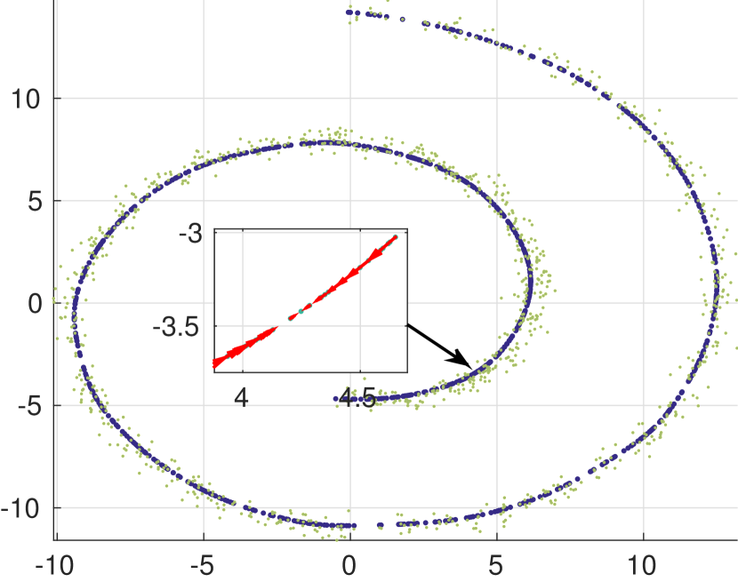
(a) Noisy one-dimensional manifold(light green) embedded in $\mathbb{R}^{2}$ and the density ridge estimate(dark blue). The small window shows a selected portion of the density ridge and the corresponding gradient flow. We can see the corresponding local maxima of the gradient flow in the figure on the left.

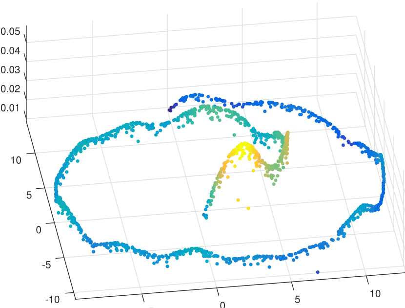
(b) Probability density along the intrinsic one-dimensional ridge from Figure 1(b) shown on vertical axis. Note that the density along the ridge has several local maxima. The points are additionaly marked with color proportional to the density value – from dark blue (low) to yellow (high) – to ease the interpretation.

Figure 1: Gradient flow and probability density along a noisy one-dimensional manifold.

It is evident that there are local maxima along the single connected ridge. Again, this observation is key to our proposition; by following the gradient flow of the density along the ridge we have a way of tracing the underlying manifold and thus calculating distances along the manifold.

Continuing to the $d$-dimensional case, the gradient flow will generate unique curves from each point on the density towards the local modes. The manifold can thus be inuitively be separated into parts based where the gradient flow converges to the same critical points. Each part can then be mapped by a linear projection approximating the logarithmic map (see for example Figure 4 on page 4 or Brun et al. (Brun et al., 2005)). In Figure 2 we see a two-dimensional manifold embedded in $\mathbb{R}^{3}$ estimated by a density ridge and the corresponding gradient flows from different views in Figure 2(b) and 2(a). In Figure 2(c) we see the sets of points, attraction basins, that have gradient flows that converge to the same point marked with similar colors. We see in Figure 2(d) that restricting the local flattening to cover only the different attraction basins separately will result in meaningful compact local representations. Flattening the entire manifold would, depending on perspective, most certainly introduce some kind of unwanted folding or collapsing.

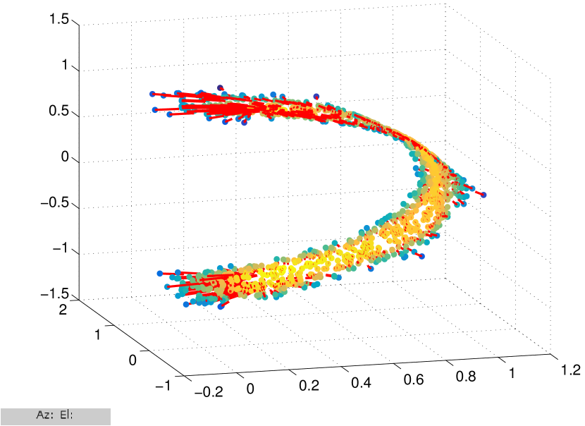
(a) Side view of manifold with gradient flow.

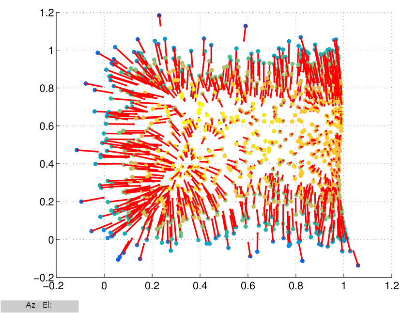
(b) Top view of manifold with gradient flow.

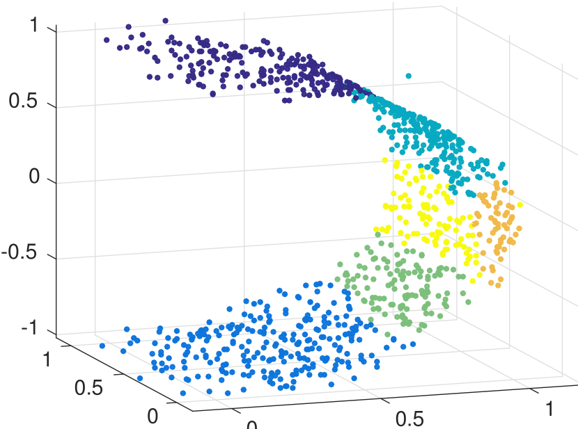
(c) Resulting attraction bases of the gradient flow.

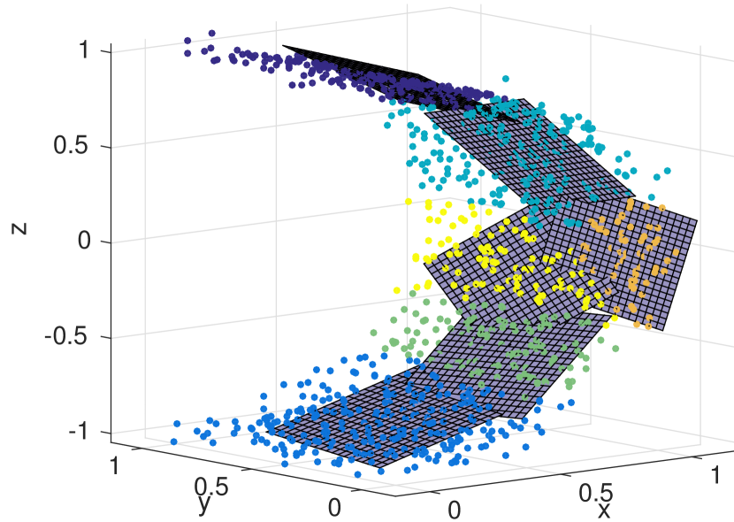
(d) Local linear flattening of attraction basins.

Figure 2: Gradient flow on a two-dimensional manifold.

Continuing from local to global unwrapping, we note that as we are using a kernel density estimate the gradient flow of the probability density is inherently local. Thus piecewise distances – or any other further operations – will also only be local, and to obtain a global unwrapping we need some strategy to combine local unwrappings. This is also clearly seen in Figure 2(d); the local attraction basins are flattened intuitively, but globally the representation is not meaningful.

To obtain a global representation we take inspiration from the concept of parallel transport from differential geometry (Lee, 1997) and introduce a translation along the tangent vectors of the one-dimensional ridges (translation along geodesics in the $d$-dimensional case) to obtain a complete unwrapped, or simply flat, representation of the ridge. This is analoguous to parallel transporting vectors along a geodesic, see for example Freifeld et al., (Freifeld et al., 2014), except that the piece-wise local distance along the geodesic is also added to the transported vector.

The result of global unwrapping of the two-dimensional manifold in Figure 2 is shown in Figure 3.

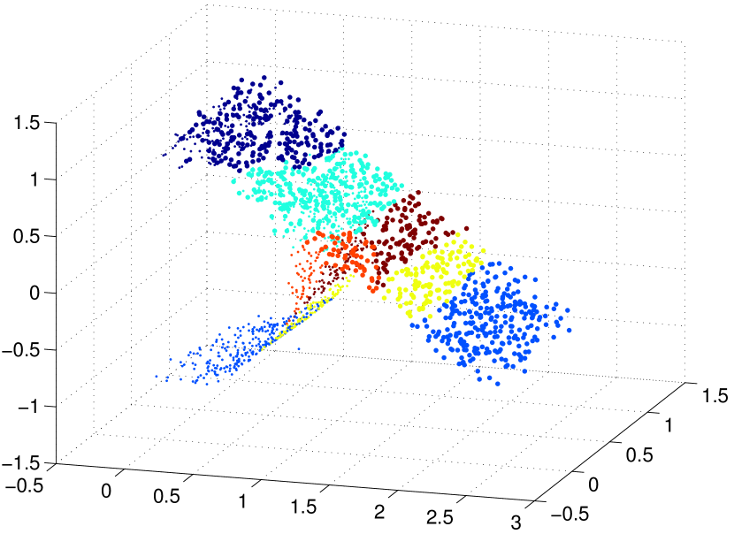
(a) Density ridge and unwrapped version. The color coding corresponds to attraction basins.

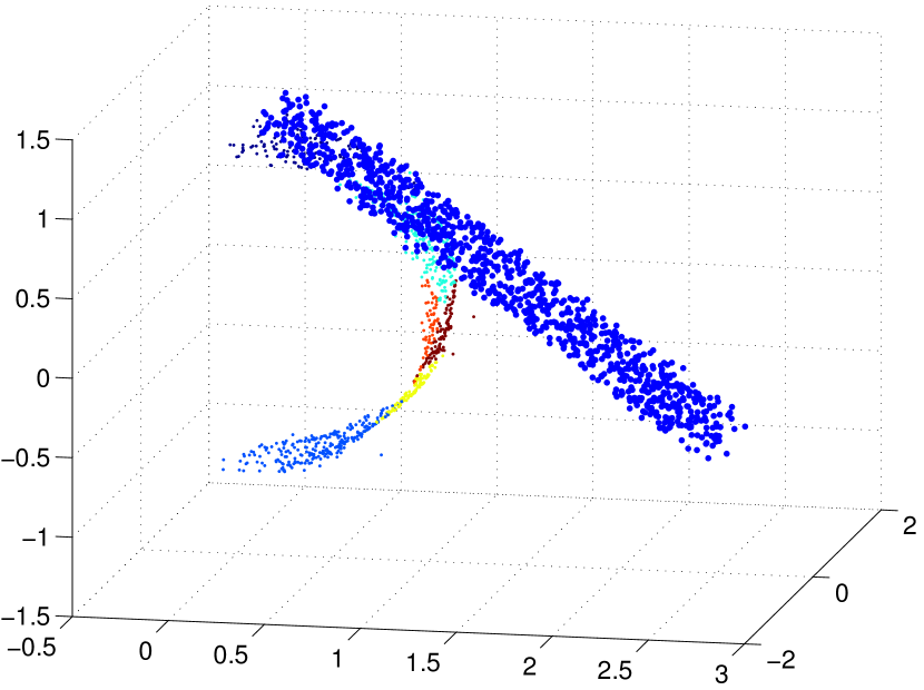
(b) Density ridge and unwrapped version. The color coding of the unwrapped manifold is kept a single color (blue) for easier visualization.

Figure 3: Unwrapped version of the two dimensional manifold in Figure 2.

To summarize, the gradient flow of a kernel density allows unwrapping manifolds using the following two steps:

1. Estimating local coordinate patches in the basins of attractions of the pdf.

2. Stitching together local coordinate charts by approximate parallel tranport/translation along geodesics.

To conclude this section we add two further comments that should be noted: (1) If the intrinsic manifold turns out to be an embedded surface ($S\subset\mathbb{R}^{2}$) or hypersurface ($S\subset\mathbb{R}^{d},\;d\geq 3$), we have to consider the case of non-zero curvature, where an isometric (distance-preserving) mapping or unfolding cannot be guaranteed. For simplicity, in the rest of this paper we assume that the manifolds we are working with are isometric to $\mathbb{R}^{d}$. (2) In some cases, the definition of the density ridges allows for multiple orthogonal one-dimensional ridges, up to $d$ if $f({\mathbf{x}}):\mathbb{R}^{d}\to\mathbb{R}$. In such cases local orthogonal coordinate systems can be estimated by first estimating the orthogonal ridges and then follow the gradient flow along each separate curve. This is useful in situations where the underlying one-dimensional manifold is corrupted by noise that changes along the manifold.

1.3 Structure of paper

The rest of the paper is organized as follows: We start by formally introducing principal curves and density ridges as in the framework of Ozertem and Erdogmus (Ozertem and Erdogmus, 2011). We then include some relevant topics from differential geometry, and show connections to density ridges as found by kernel density estimation in Section 3. In Section 4 we present the principal curve/one-dimensional density ridge unwrapping algorithm followed by the ridge translation algorithm in Section 5. Section 6 proposes extensions to density ridges of higher dimension and finally in Section 7 we show numerical examples and illustrations of the presented methods on both synthetic and real datasets.

2 Principal curves and density ridges

Principal curves were originally introduced by Hastie and Stuetzle (Hastie and Stuetzle, 1989). Several extensions were made, (Kégl et al., 2000; Einbeck et al., 2005; Tibshirani, 1992), until Ozertem and Erdogmus, (Ozertem and Erdogmus, 2011), redefined principal curves and surfaces as being the ridges of a probability density estimate, (Ozertem and Erdogmus, 2011). Given a probability density $f({\mathbf{x}})$, its gradient $g({\mathbf{x}})=\nabla^{T}f({\mathbf{x}})$ and Hessian matrix $H({\mathbf{x}})=\nabla\nabla^{T}f({\mathbf{x}})$, the ridge can be defined in terms of the eigendecomposition of the Hessian matrix.

Definition 1 (Ozertem 2011)

A point ${\mathbf{x}}$ is on the $d$-dimensional ridge, $R$ of its probability density function, when the gradient $g({\mathbf{x}})$ is orthogonal to at least $D-d$ eigenvectors of $H({\mathbf{x}})$ and the corresponding $D-d$ eigenvalues are all negative.

We express the spectral decomposition of $H$ as $H({\mathbf{x}})=Q({\mathbf{x}})\Lambda({\mathbf{x}})Q({\mathbf{x}})^{T}$, where $Q({\mathbf{x}})$ is the matrix of eigenvectors sorted according to the size of the eigenvalue and $\Lambda_{ii}({\mathbf{x}})=\lambda_{i}$, $\lambda_{1}({\mathbf{x}})>\lambda_{2}({\mathbf{x}})>\dots$, is a diagonal matrix of sorted eigenvalues. Furthermore $Q({\mathbf{x}})$ can be decomposed into $\left[Q_{\perp}({\mathbf{x}})\;Q_{\parallel}({\mathbf{x}})\right]$, where $Q_{\perp}$ is the $d$ first eigenvectors of $Q({\mathbf{x}})$, and $Q_{\parallel}$ are the $D-d$ smallest. The latter is referred to as the orthogonal subspace due to the fact that when at a ridge point, all eigenvectors in $Q_{\perp}$ will be orthogonal to $g({\mathbf{x}})$.

This motivates the following initial value problem for projecting points onto a density ridge:

$$\frac{\text{d}\mathbf{y}_{t}}{\text{d}t}=V_{t}V_{t}^{T}g(\mathbf{y}_{t}),$$ (1)

where $V_{t}=Q_{\perp}({\mathbf{x}}(t))$ at $\mathbf{y}_{t}=\mathbf{y}(t)$, and $\mathbf{y}(0)=\mathbf{x}$. We denote the set of $\mathbf{y}$’s that satisfy equation (1), calculated via the kernel density estimator $\hat{f}({\mathbf{x}})$, as the $d$-dimensional ridge estimator $\hat{R}$.

Of great value is the recent paper by Genovese et al., (Genovese et al., 2014), which showed that the Hausdorff distance between a $d$-dimensional manifold embedded in $D$ dimensions and the $d$-dimensional ridge of the density is bounded under certain restrictions wrt. noise and the closeness of the density estimate to the true density. They also show that the kernel density ridges are consistent estimators of the true underlying ridges and refer to the ridge as a surrogate of the underlying manifold. Thus, $\hat{R}$ is a point set representing the underlying manifold with theoretically established bounds under Hausdorff loss.

2.1 Orthogonal local principal curves

In the special case of a projection onto a principal curve, $d=1$, we note that the construction of the orthogonal subspace allows for choosing $d$ different orthogonal subspaces to project the gradient to. The most intuitive setting, which is most commonly used (Ozertem and Erdogmus, 2011; Genovese et al., 2014; Bas, 2011) is to use the top eigenvector(s) corresponding to eigenvalue(s) as the orthogonal subspace. We recall that the eigenvalues and eigenvectors of the Hessian matrix of a function points to the directions of largest second order change. In the case of a density ridge, the change in density along the ridge is assumed to be much lower than the change in density when moving away from the ridges, hence the choice of largest eigenvector pointing away from the ridge. This local ordering, though intuitive from the Hessian point of view, has not been well studied, and could in some cases actually give non-intuitive results. We will not go further into this in this paper.

The importance of this local decomposition is that considering a $d$-dimensional ridge, the ridge tracing algorithm, presented in Section 4, can be applied on each of the local orthogonal subspaces. In the case of e.g. different local scales of noise this could yield a better desciption of the data. Figure 4 shows a conceptual illustration of the idea, where the overall dominating nonlinearity can be described by a principal curve/one-dimensional density ridge, but since the orthogonal structure varies along the ridge local decomposition provides further detail.

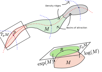
Figure 4: A manifold with a one-dimensional ridge/principal curve. The local basins of attraction can be decomposed using orthogonal principal curves. $M$ is the intrinsic manifold, $T_{p}M$ denotes the tangent space of $M$ at $p$. The green area denoted in the lower right sketch is the area of $T_{p}M$ constrained by the exponential map.

3 Relevant topics from differential geometry

Manifold learning is a framework which is inspired by concepts from differential geometry (Brun et al., 2005; Tenenbaum et al., 2000; Pitelis et al., 2013; Roweis and Saul, 2000; Gerber and Whitaker, 2013; Zhang and Zha, 2004). The main idea is that data sets or data structures seldom fill the vector space they are represented in. Even in low dimensions, e.g. $\mathbb{R}^{3}$, data often concentrate around clearly bounded subregions or so-called manifolds.

In some works the problem of learning representations on or along a manifold has been termed manifold unwrapping or unfolding (Weinberger and Saul, 2006; Sun et al., 2012). The idea is that learning the structure of a manifold keeps the local structures intact more strongly than global structures, so that the (global) nonlinearities can be unfolded, unrolled or unwrapped. This is perhaps the term most related to our work.

Unfolding or unwrapping a manifold can intuitively be performed in two different ways. Either we use some function that stretches or flattens the manifold such that we can use linear methods to calculate distances along the manifold, or we can somehow estimate the structure of the manifold such that distance measures can be defined directly along the manifold again allowing linear operations in the resulting coordinate system.

The ideas and concepts of manifold learning stems from differential geometry, the field of mathematics which studies smooth geometric objects and, closely related, smooth functions. Its main object of interest is the manifold, which can be roughly regarded as a well behaving smooth (topological) space.

A clear definition of a manifold can be found in either books of Lee or Tu, (Lee, 1997; Tu, 2008):

Definition 2

A (topological) manifold is a second countable, locally Euclidean, Hausdorff space.

Local Euclidean structure is analoguous to how humans perceive the surface of the earth. At smaller scales traversing a path along the surface will seem like a straight line, but on larger scales paths along the surface of the earth are clearly curved. A Hausdorff space is a space where two separate points have disjoint neighboorhoods (Barile and Weisstein, ). E.g. a surface embedded in $\mathbb{R}^{3}$ that intersects with itself will have points that shares neighborhoods and is thus not Hausdorff.

In simple terms; the intuition behind differential geometry and manifolds is to describe an object locally at a certain point or a certain homogenuous region using derivatives. Although often not explicitly stated the kernel density estimate and its derivatives – see e.g. (Chacón et al., 2013) – can be interpreted in a differential geometry setting. We recall that Genovese et al., (Genovese et al., 2014), has shown that kernel density derivatives can be used to estimate a smoothed version of an underlying manifold sampled from data with noise.

Before we go into further discussion of the connection between the kernel density estimate of data sampled from a manifold and differential geometry, we introduce a few basic concepts.

First: throughout this discussion we are talking about submanifolds of $\mathbb{R}^{D}$ (Lee, 1997). Given a manifold $M$ diffeomorphic to $\mathbb{R}^{d}$, at each point $p\in M$ the tangent space, $T_{p}M$, is the Euclidean space of dimension $d$ which is tangent to $M$ at $p$ (Lee, 1997). See Figure 4 for a sketch of the related concepts. The term tangent to, can intuitively be interpreted as either the space of tangent vectors of all possible curves passing through $p$ or the space spanned by the partial derivatives of the parametrization of $M$ at $p$ (Lee, 1997). A disjoint union of all tangent spaces of $M$ is called the tangent bundle. We denote the coordinate transformation from the tangent space $T_{p}M$to the manifold $M$ as the exponential map, and the inverse transformation from the $M$ to the $T_{P}M$ as the log map (Brun et al., 2005). Finally we note that vectors in $T_{p}M$ can be expressed by a local basis of differentials $E_{i}=\frac{\partial p}{\partial x^{i}}$. These are called the local coordinates at $p$, (Lee, 1997). These local coordinates represents a Euclidean subspace of same dimension $d$ as $M$.

As for the statiscal model, we assume the same model as in (Genovese et al., 2014) where the data points, $X=\left\{{\mathbf{x}}_{i}\right\}_{i=1}^{n}\in\mathbb{R}^{D}$, are sampled with noise from a distribution supported on $M$. If we let $P_{M}$ be the distribution of points on and along $M$ and $\Phi_{\sigma}$ be a Gaussian distribution with zero mean and $\sigma I$ covariance – also in $\mathbb{R}^{D}$ – that represents noisy samples that does not lie directly on the manifold, we get the following model:

$$P=P_{M}*\Phi_{\sigma}.$$

The kernel density estimator is defined as follows:

$$\hat{p}({\mathbf{x}})=\frac{1}{n}\sum^{n}_{i=1}\frac{1}{\sigma^{2}}K\left(\frac{||{\mathbf{x}}-{\mathbf{x}}_{i}||}{\sigma^{2}}\right),$$ (2)

where $K(\cdot)$ is any symmetric and positive semi-definite kernel function. Note that we skip the normalizing constant, as it is simply a matter of scale and we are only interested in the direction of the gradient and the Hessian eigenvectors. We also note that in this work we restrict ourselves to use the Gaussian kernel $K({\mathbf{x}}_{j},{\mathbf{x}}_{i})=\exp(-||x_{i}-x_{j}||^{2}/2\sigma^{2})$. From the kernel density estimate we can calculate the gradient as follows(notation adapted from (Genovese et al., 2014)):

$$g({\mathbf{x}})=-\frac{1}{n}\sum^{n}_{i=1}\frac{{\mathbf{x}}-{\mathbf{x}}_{i}}{\sigma^{2}}K\left(\frac{||{\mathbf{x}}-{\mathbf{x}}_{i}||}{\sigma^{2}}\right).$$ (3)

And finally the Hessian matrix:

$$H({\mathbf{x}})=\frac{1}{n}\sum^{n}_{i=1}\left(\mathbf{u}_{i}\mathbf{u}_{i}^{T}-\frac{1}{\sigma^{2}}I\right)K\left(\frac{||{\mathbf{x}}-{\mathbf{x}}_{i}||}{\sigma^{2}}\right),$$ (4)

where $\mathbf{u}_{i}=({\mathbf{x}}-{\mathbf{x}}_{i})$. From these equations we see that the gradient is simply the average of all vectors pointing out from ${\mathbf{x}}$ weighted by the kernel function value of the norm of the vectors. We also note that depending on the kernel size $\sigma^{2}$ the gradient will in practice be the average of the vectors pointing from ${\mathbf{x}}$ to all points within the neighborhood covered by the particular kernel size. If a point and its neighbors within the kernel size distance lies on or close to the manifold $M$, this clearly is a good candidate for a local tangent space estimate.

If we look at the expression for the Hessian matrix, we notice that it turns out to be proportional to the sample covariance matrix at $x$ with the variance normalized wrt the kernel size $\sigma^{2}$. Like the kernel density gradient, the weight of the points taken into account in calculating the covariance is governed by the kernel size, leading to a local sample covariance estimate at ${\mathbf{x}}$. We note that if a very large kernel size, in the order of $\operatorname{var}\{X\}$, is used, the Hessian matrix will resemble the standard sample covariance matrix and eigendecomposition would yield standard PCA. Considering this we can interpret the Hessian matrix as fixing and aligning a local Gaussian distribution to a local subset of the data. For a one-dimensional curve with multidimensional additive noise the local Gaussian will clearly have a strong correlation along the curve wich will be reflected in the eigenvectors of the local Hessian estimate. A simple illustration of this is shown in Figure 5. Considering the case of a principal surface we can continue our principal component analogy. Assuming the points have been sampled from some surface with some level of noise, the kernel density Hessian estimate at ${\mathbf{x}}$ will in practice calculate a covariance matrix estimate based on the points within the range covered by the kernel centered at ${\mathbf{x}}$. Unless the noisy points that does not lie on $M$ completely dominate, we expect that most of the variance is concentrated along the manifold, and thus the largest eigenvectors according to eigenvalue will span the local tangent space $T_{\mathbf{x}}M$.

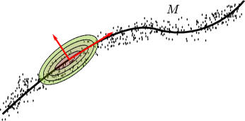
Figure 5: Illustration of the eigenvectors (red arrows) of the kernel density Hessian matrix at a point on the manifold $M$ (thick black line). A figurative illustration of the contours of the kernel centered at the same point is also shown to illustrate the bandwidth of the kernel.

Since by definition the kernel density gradient, $g({\mathbf{x}})$, lies in the span of $d$ Hessian eigenvectors if ${\mathbf{x}}$ is on the $d$-dimensional ridge, the corresponding $d$ eigenvectors forms a natural basis for local coordinates in $T_{\mathbf{x}}M$. Consequently the parallel Hessian eigenvectors, $Q_{||}$, can be calculated for each ${\mathbf{x}}$ that lies on the density ridge, also for out of sample points, and will thus form an approximate tangent bundle on the ridge estimate of the manifold, $\hat{R}$.

3.1 Properties of density ridges

Throughout this section we consider a single connected submanifold $M$ of Euclidean space without boundary that satisifies the properties given in (Genovese et al., 2014).

Recall that a principal curve can be approximated by a one-dimensional density ridge and a principal surface by a $d$-dimensional density ridge. Some properties are general, while some apply only to principal curves, or vice versa. We start by introducing the gradient flow, which we use in both cases later in this paper.

An integral curve of the positive gradient flow is a curve $\lambda(t)$ such that $\lambda^{\prime}(t)=\nabla f(\lambda(t))$. For every point $x_{0}$ in the domain of $f$ there exists an integral curve that starts at $x_{0}$. Given a critical point $\mathbf{m}$, $\nabla(\mathbf{m})=0$, all points that have integral curves that converges to the critical point are said to lie in the basin of attraction of $\mathbf{m}$ (Arias-Castro et al., 2013). This property is the foundation of mode based clustering algorithms, e.g mean shift clustering (Comaniciu and Meer, 2002; Myhre et al., 2015).

The idea of a basin of attraction can be extended to hold for density ridges as well. Given a density ridge of dimension $d$ a local mode will still satisfy the criteria for being a point on the ridge. The differential equation – equation (1) on page 1 – for projecting points towards the density ridge always follows the gradient, so the density ridge(s) can be divided into basins of attraction based on the original points before projection. This naturally divides a manifold estimated by a density ridge into non-overlapping subsets. Closely related: a chart of a smooth manifold is a diffeomorphism from a neighborhood $U$ on the manifold to $V\subset\mathbb{R}^{d}$, $\phi:U\to V$. The local density ridge unwrapping algorithm, presented in Section 4 can be considered an algorithm for learning the map $\phi$, and we thus have a chart for each separate basin of attraction of the manifold. We note that in classical differential geometry it is common to consider smoothly overlapping charts (Tu, 2008), which is not the case in this work.

We end this section with a short summary of important properties and observations for principal curves and surfaces separately.

Principal curves:

• The gradient flow integral curves $\gamma$ are geodesics, allowing for parallel transport, this will be introduced in Section 5.

• The gradient flow separates the manifold into non-overlapping regions $C_{i}$ - attraction basins, such that $M=\bigcup\limits_{i=1}^{\#\text{charts}}C_{i}$

• Curves does not have intrinsic curvature, and thus principal curves can always be unfolded isometrically.

• $T_{{\mathbf{x}}}M=\operatorname{span}\left(g({\mathbf{x}})\right)$, $g({\mathbf{x}})=\lambda Q_{\parallel}({\mathbf{x}})$. Thus, the gradient flow curve starting on points on the manifold is completely contained along the one-dimensional manifold, $\gamma\in M$.

Principal surfaces:

• The gradient flow separates the manifold into non-overlapping regions - attraction basins. Again $M=\bigcup\limits_{i=1}^{\#\text{charts}}C_{i}$.

• The gradient flow curves $\gamma$ are not necessarily geodesics. If the initial point is on the manifold the gradient flow integral curves will be restricted to the manifold. Thus, if $\gamma(0)\in M$, $\gamma(t)\in M\>\;\forall{t}$.

• Curvature must be introduced, isometric unfolding can no longer be guaranteed for arbitrary surfaces.

• $T_{{\mathbf{x}}}M=\operatorname{span}\left(Q_{\parallel}({\mathbf{x}})\right)$. Thus the direction of the gradient determines the gradient flow along the manifold.

4 Proposed method: Principal curve unwrapping by tracing the ridge

In this section we present the first part of our suggested algorithm for unwrapping manifolds, which deals with data distributed on and along a one-dimensional manifold. We start by recalling that the probability density function along a local principal curve/one-dimensional density ridge will contain local maxima. For a point ${\mathbf{x}}\in\hat{R}$ the gradient, $g({\mathbf{x}})$, is by definition orthogonal to all except one of the eigenvectors of the local Hessian $H({\mathbf{x}})$. Thus any gradient on the ridge which is not exactly zero will point along the ridge towards a local mode. This restricts the gradient flow, (Arias-Castro et al., 2013), along the ridge to stay on the ridge, and thus we can formulate a differential equation that sends the points on the principal curve, along the curve/ridge towards the local mode. We note that Arias-Castro et al. showed that a gradient ascent scheme for estimating the gradient flow lines converges uniformly to the true integral curve lines (Arias-Castro et al., 2013). Then, by using either a gradient ascent scheme – like in mean shift clustering – or as in this work a differential equation solver, we can estimate the gradient flow lines along a ridge, and by calculating the piece-wise Euclidean distances between the steps of the gradient flow we can estimate the distance from a point to a local mode along the ridge. Since this is the only possible path between the point on the ridge and the local mode it converges to, it is by construction a geodesic. These geodesic distances along the principal curve we will take as local coordinates in the basin of attraction of the local mode, $\mathbf{m}_{i}$, with the smallest eigenvector of $H(\mathbf{m}_{i})$ as basis. We state the differential equation for following the gradient along the ridge as follows:

$$\frac{\text{d}\mathbf{z}(t)}{\text{d}t}=g(\mathbf{z}(t)),$$ (5)

where $\mathbf{z}(0)=\mathbf{y}(T)$, $T$ such that $V_{T}^{T}g(\mathbf{y}_{T})\approx 0$.

Solving this equations gives coordinate lengths along the ridge and thus yields a complete local coordinate description for every point in the local basin of attraction of $\mathbf{m}_{i}$.

Algorithm 1 Local density ridge unwrapping.

0:  Input points, ${\mathbf{x}}_{i}$, projected to a one-dimensional density ridge $\hat{R}$ by solving Equation (1).

1:  Compute the trajectory, $Z_{i}$, from each point on the density ridge to the associated mode by solving Equation (5).

2:  For each trajectory $Z_{i}=\begin{bmatrix}\mathbf{z}_{i}^{1}&\mathbf{z}_{i}^{2}&\cdots&\mathbf{z}_{i}^{N}\end{bmatrix}$ calculate:

$$\mathbf{c}_{i}=\sum^{N-1}_{j=1}\|\mathbf{z}_{i}^{j}-\mathbf{z}_{i}^{j+1}\|_{2}$$ (6)

2:  Local manifold chart coordinate $\mathbf{c}_{i}$.

In practice we solve this using a Runge Kutta fourth and fifth order pair, also known as the Runge-Kutta-Fehlberg method(RKF5) (Fehlberg, 1969), implemented in MATLAB. This is an adaptive stepwise solver, which yields benefits both in terms of speed and accuracy. For density ridge estimations we use the kernel density estimate from Equation (2), its gradient, Equation (3), and the Hessian matrix from Equation (4) as presented in the previous section. The ridge projection for each data point considered is independent from other projections, so processing each point in parallel is possible. In this work we have used the parallel processing toolbox in MATLAB to achieve a local speedup proportional to the number of cores on the computer.

We have summarized the steps necessary to perform local principal curve unwrapping in Algorithm 1.

We conclude this section with an illustration of Algorithm 1. In Figure 6 we see a two dimensional sample from a Gaussian distribution superimposed with an underlying one-dimensional nonlinear structure. The two orthogonal density ridges found using the RKF45 solver are shown in red and blue dotted lines.

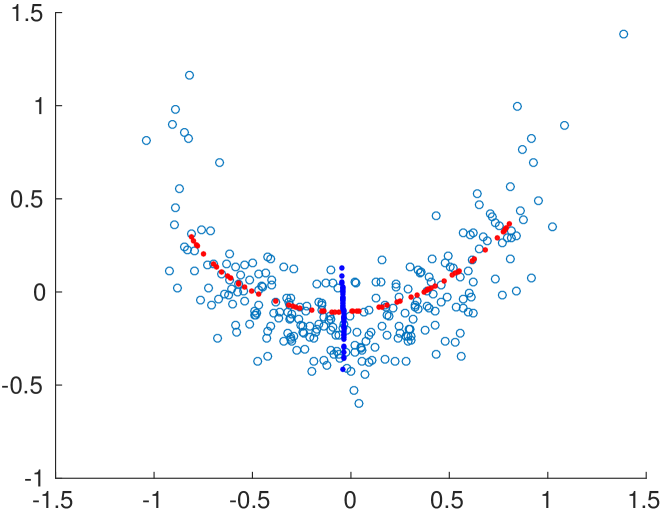
Figure 6: Nonlinear and noncovex data set with density ridges shown in red(top) and blue(second).

In Figure 7 we see the stages in Algorithm 1 for a single data point from Figure 6. First the point is projected to each of the two orthogonal density ridges using the RKF45 algorithm, shown in red. Second, the point is projected along the ridge by following the gradient towards the local mode shown in green. We see that by calculating the piece-wise Euclidean distances between the gradient ascent steps – the green points – we get approximate coordinate distance along the intrinsic nonlinear geometry.

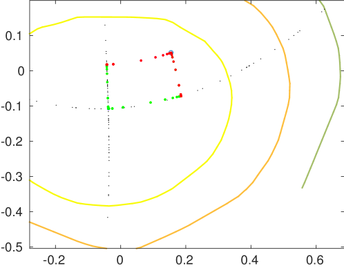
Figure 7: A single data point projected to the two one-dimensional density ridges, trajectories shown in red and then along the gradient to the local mode(green). The density ridges as shown in Fig 6 are marked with small black dots.

5 Parallel transport along density ridges

The local density ridge unwrapping algorithm presented in the previous section is only valid for local regions of the manifold. This implies that the local unwrapping algorithm can result in several charts for a single connected manifold if there are multiple local maxima along the ridge. So given a manifold $M$ embedded in $\mathbb{R}^{d}$ and a ridge approximator $\hat{R}$ consisting of a set over non-overlapping attraction bases, we can, by using Algorithm 1, obtain a local coordinate chart for each of the local attraction basins.

In the current setting where the underlying manifold describing the nonlinearity can be described by a one-dimensional ridge, the trajectories along the manifold can trivially be considered geodesics. This allows the use of parallel transport to transport vectors from one mode to another if they are connected by a principal curve/one-dimensional ridge Lee (1997). In this work we will not go further into the differential geometric framework for parallel transport – see for example (Lee, 1997) – , but rather develop a discrete empirical algorithm for sewing together local charts stemming from Algorithm 1 by translation along geodesics.

We make the following assumptions:

• If there is a one-dimensional ridge between two local modes, it can by definition be considered a geodesic.

• The local neighborhood around a density mode can be described by trajectories along local orthogonal density ridges.

To form a global representation of a manifold $M$, we need to relate the coordinate charts of the manifold to each other.

To do this we select a reference mode along the principal curve and translate the other local coordinate systems connected to the same ridge towards the reference mode. This is a straight forward operation, but there are a few issues that needs to be considered. First, each local system needs a basis and consequently the bases along the curve needs to be checked in case they are not equally aligned to the ridge. Second, once a reference mode and basis is chosen, the translation of other charts towards that mode can give ambiguities in terms of sign, if two charts are translated towards the same mode from different directions, a positive and negative direction needs to be defined.

Given a manifold $M$ and its ridge estimator $\hat{R}$, the set of local modes, $\left\{\mathbf{m}_{i}\right\}_{i=1}^{m}$, along the ridge, the gradient and Hessian at each point in both $\hat{R}$ and $\left\{\mathbf{m}_{i}\right\}_{i=1}^{m}$, we define the following:

Definition 3

At a given a reference mode $\mathbf{m}_{r}$, we define the $d$ eigenvectors of the Hessian of the kernel density estimate at $\mathbf{m}_{r}$ as the basis of the unwrapped coordinates.

Using this we can check the sign of the determinant of the other bases along $\hat{R}$ and change signs if the bases have a different orientations. This ensures a consistens orientation, unless the manifold is not orientable (e.g. a Möbius strip) (Spivak, 1965).

Definition 4

Given a reference mode $\mathbf{m}_{r}$, we define the direction towards the closest local mode along the ridge $\hat{R}$ as the positive direction.

As the ridge connecting two local modes is one-dimensional, tangent vectors by finite differences from mode to reference mode can be used to identify the relevant directions. Even though the ridge estimate $\hat{R}$ and local modes are known, we do not know if two local modes are connected and the order of the points contained in a local attraction base. As preliminary solutions to this, we use Dijkstra’s algorithm for identifying the path along the ridge from mode to mode, and use that path to calculate finite difference tangent vectors (Dijkstra, 1959). To check if two modes are connected we use the flood fill algorithm (Heckbert, 1990). Both algorithms operate on a nearest neighbor graph which in this case consists of the every input point projected to the density ridge estimator as well as the set of local modes found by following the gradients along the ridge for all points. The flood fill algorithm simply checks the number of connected components in a graph. Thus if there are several components along a one-dimensional density ridge, either the neighborhood graph must be expanded or the ridge is disconnected. Dijkstras algorithm calculates the shortest path along nodes in a sparse graph. In ridges of dimension higher than one, this would lead to poor estimates, but since all points along the one-dimensional ridges lie on a curve this is not a problem. In practice, the Dijkstra algorithm ends up simply sorting the points along the density ridge. Thus we have all steps needed to translate a local chart along the connecting density ridge and obtain a global unwrapping. The density ridge translation algorithm is summarized in in Algorithm 2.

Algorithm 2 Density ridge translation algorithm

0:  Ridge estimator $\hat{R}$, local modes $\mathbf{m}_{i}$ and unwrapped coordinates $\mathbf{c}_{i}$ corresponding to each local mode.

1:  Create a nearest neigborhood graph consisting of $\left\{\mathbf{m}_{i}\right\}_{i=1}^{m}$ and $\hat{R}$.

2:  Select a reference mode, $\mathbf{m}_{r}$, and calculate the geodesic path, $\gamma_{i,r}(t)$to all other modes $\mathbf{m}_{i}$ along the ridge using Dijkstras algorithm.

3:  Chose the mode closest to $\mathbf{m}_{r}$ and define the direction along $\hat{R}$ towards that mode as the positive direction.

4:  for all Local coordinate charts, $\mathbf{c}_{i}$ do

5:     Calculate fininite difference tangent vectors along the geodesic path, $t_{l}=\gamma_{i,r}(t_{l})-\gamma(t_{l-1})$.

6:     Select the coordinate direction of the translation. E.g. the first coordinate if translation is along the first principal curve/density ridge.

7:     Translate the local coordinates along the geodesic by adding the tangent vector length to the chosen coordinate direction.

$$\mathbf{c}_{translated}=\sum_{l}\mathbf{c}_{i}^{j}+||t_{l}||$$ (7)

8:  end for

9:  Concatenate all translated charts into a global representation $\mathbf{Z}$.

9:  Global representation, $\mathbf{Z}$ of concatenated and connected charts.

We end this section with an example. In Figure 8(a) and Figure 8(b) we see a two-dimensional uniform sample superimposed with a nonlinear structure, its density and one-dimensional orthogonal density ridges. The color coding of Figure 8(a) represents the order of the data points in the horizontal direction.

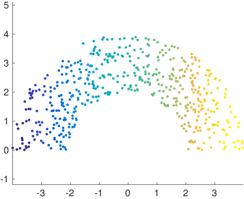
(a) Uniform data perturbed with a nonlinear shape.

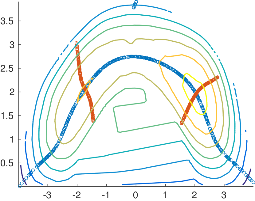
(b) Nonlinear uniform data set with kernel density estimate contours and orthogonal one-dimensional ridges shown.

Figure 8: Nonlinear uniform data set.

Figure 9 shows the results of the density ridge translation algorithm. We see that the underlying uniform distribution is revealed. There are some artifacts at the boundary of the manifold, this is probably due to the smoothness of the kernel density estimate and the fact that the kernel density estimate is close to a mixture of two Gaussians. There will always be a tradeoff between bias in the principal curves and non-smooth, but well fitting ridges. In other words, the smoother the curve, the larger the bias and the closer the density is to a mixture of a low number of Gaussians .

Figure 9: Result after applying the density ridge translation algorithm on dataset shown in Figure 8(a). Color coding follows from input data set.

We also have to note that the origin of the data structure has been moved to $\left[0,0\right]^{T}$. This is due to the arbitrary choice of reference mode. One could keep the original reference mode as origin of the unwrapped representation, but this would not affect the result other than a translation.

6 Expansion to $d$-dimensional ridges

In the case where the underlying manifold cannot be described by a principal curve, a density ridge of higher dimension, a principal surface, must be considered. This causes a problem with our previous approach: the gradient, $g({\mathbf{x}})$, of a point on a $d$-dimensional ridge lies in the span of $d$ eigenvectors of $H({\mathbf{x}})$ such that following the gradient flow will not lead to unique coordinates on the manifold. So for example applying Equation (5) on a $d$-dimensional ridge would lead to a ridge-constrained mean shift, i.e. gradient flow trajectories that lies completely on the ridge. Depending on how the data is distributed along the manifold as well as geometric properties such as curvature, a $d$-dimensional ridge cannot in general be decomposed into $d$ orthogonal one-dimensional ridges.

Also, in general, the curvature of the manifold has to be considered in higher dimensions – we can no longer be sure that an isometric unfolding exists. Furthermore, comparing with the previous section, a path between two points is also not necessarily a geodesic even if the path lies completely on the manifold. Thus the parallel transport/translation analogy cannot be directly used.

Based on the aforementioned, we propose an alternative unwrapping scheme for the density ridge framework in the case of $d$-dimensional nonlinear structures. We recall that in the one dimensional case we unfold local charts of the density ridge, and if there are several charts, transport them along the ridge to get a global representation. In the $d$-dimensional case we cannot directly unfold the local charts by following the gradient flow, so we insted do a local linear approximation by projecting the data points in the local basin of attraction to the tangent space of the local mode of the chart, presented in Section 6.1. Once we have linear approximations of all local charts of the manifold we calculate approximate geodesics and use parallel transport to send all charts to a reference mode. Finally, the unwrapping is done by sending the charts back along the geodesic by parallel transport, while at the same time constraining the piece-wise steps of the geodesic to lie in the tangent space of the reference mode, presented in Section 6.3. To approximate the geodesic we use an algorithm proposed by Dollár et al. (Dollár et al., 2007), presented in Section 6.2.

6.1 Local linear approximation

As calculating distances along gradient lines that cover the $d$-dimensional manifold will not give consistent orthogonal coordinates we will expand our approach and use local linear approximations. The approximations will consist of a local flattening centered at the local modes of the $d$-dimensional density ridge. By flattening at the local modes we get charts centered at the points of highest probability and the points within the chart are points where the gradient flow converges to the same mode. This ensures that the charts represents points that are close in density and that the charts are limited in extension since the gradient flow lines are restricted to locally smooth areas of the manifold. Following this, the flattening process consists of projecting the data points corresponding to a local mode to the space spanned by the Hessian eigenvectors that span the gradient (the local tangent space):

$$\mathbf{c}_{i}=Q_{||}(\mathbf{m}_{i})Q_{||}(\mathbf{m}_{i})^{T}\mathbf{x}_{i},$$ (8)

where $\mathbf{c}_{i}\in Q_{||}$ is a local coordinate for a point $\mathbf{x}_{i}$ that has converged to mode #$i$, $\mathbf{m}_{i}$. This is equivalent to an approximate inverse exponential map on the manifold at $\mathbf{m}_{i}$ – the log map. In this manner we get a local linear approximation for each local mode in the data set.

Also, comparing with the previously noted similarities between the Hessian of the KDE estimate and the local sample covariance matrix, we can view this local flattening directly as local PCA where the neighborhood is determined by the coverage of the kernel bandwidth.

6.2 Approximating geodesics

To obtain a global coordinate representation on a connected manifold that has a set of approximated local coordinate charts we proposed parallel transport of tangent space coordinates towards a reference mode. In the one-dimensional case a geodesic was directly available in the principal curve. In the $d$-dimensional case we need a numerical scheme to approximate the geodesic. In this paper we reframe an idea presented by Dollár et al. (Dollár et al., 2007), to approximate geodesics on the manifold. The idea is to minimize the distance between two points, while at the same time keeping the starting points and endpoints fixed and making sure that all points on the path lies approximately on the manifold. Formally, given a sequence of points $\left\{\gamma_{i}\right\}_{i=1}^{n}\in M$ between two points on the manifold ${\mathbf{x}}$ and $\mathbf{y}$ we can formulate the problem of finding a shortest path constrained to the manifold as follows:

$$\underset{\gamma}{\text{minimize}} \sum^{n}_{l=2}||\gamma_{l}-\gamma_{l-1}||^{2}$$ (9)

subject to $$\gamma_{1}={\mathbf{x}},\;\gamma_{n}=\mathbf{y},\;\gamma\in M.$$

To optimize (9) the path $\gamma$ is initialized using Dijkstra’s algorithm and further discretized with linear interpolation between the $n$ given points. Then minimization is performed by alternating between gradient descent to shorten distance and density ridge projection, equation (1) to ensure that points stay on the manifold. In addition we use another idea from the work of Dollár et al. (Dollár et al., 2007) for fast out of sample projections. After a selection of points have been projected to the density ridge, by equation (1), the tangent space of the ridge estimator is at each point ${\mathbf{x}}$ spanned by the parallel Hessian eigenvectors $Q_{\parallel}({\mathbf{x}})$. To project a new out-of-sample point ${\mathbf{x}}_{o}$ orthogonally to the ridge, $||{\mathbf{x}}_{o}-{\mathbf{x}}_{r}||^{2}$, where ${\mathbf{x}}_{r}$ is a point on the ridge, needs to be minimized. This can be solved by setting ${\mathbf{x}}_{r}$ to the closest point of ${\mathbf{x}}_{o}$ on the manifold and then performing gradient descent as follows:

$${\mathbf{x}}_{r}\leftarrow{\mathbf{x}}_{r}+\alpha Q_{\parallel}({\mathbf{x}}_{r})Q_{\parallel}({\mathbf{x}}_{r})^{T}\left({\mathbf{x}}_{o}-{\mathbf{x}}_{r}\right)$$ (10)

An illustration of the geodesics found by the alternating optimization of equations 9 and 10 on the ‘swiss roll’ dataset, (Tenenbaum et al., 2000), is shown in Figure 10.

Figure 10: Swissroll dataset showing two different geodesics approximated by the alternating least squares scheme in equation (9).

6.3 Combining geodesics and local approximations

Once we have local approximations in place we can in principle directly unfold manifolds that are isometric. We recall that if a manifold is isometric it has no intrinsic curvature and can be covered by a global chart, in other words: the diffeomorphism $\phi:\mathbb{R}^{d}\to M$ preserves distances. Still, if we use the algorithms presented previously in this paper we cannot in general find a single global chart. Combining the two previous sections we have the following: an estimate of the underlying density ridge $\hat{R}$ which is close to the true manifold, a set of local linear approximations $C$ of each local basin of attraction and the possibility of estimating geodesics between points in $\hat{R}$ by Equation (9).

Using these tools we can construct an algorithm for stitching together the local approximations $C$ to obtain a global unwrapping. Below we present a short outline of the algorithm, see the appendix for a complete description of the algorithm:

1. For each mode, project the points in the local attraction basin to the space spanned by the parallel Hessian eigenvectors.

2. Among all modes, select a reference mode and calculate the piece-wise geodesic distance from all other modes to the reference mode

3. Transport the local approximations towards the reference mode by iteratively translating and projecting to the local tangent space along the geodesics. Algorithm 3 is presented in Appendix A.

4. Once all coordinates are centered on the reference mode send them along the tangent vector of the reversed geodesic projected to the local tangent space of the reference mode. This is presented in Algorithm 4 in Appendix B.

We conclude this section with a short example. Again we turn to the swiss roll example, where a plane is deformed into a swiss roll shape embedded in $\mathbb{R}^{3}$. See Figure 23 for the data and unwrapped result.

7 Numerical experiments

We now show a selection of experiments to illustrate the presented frameworks. Both real and synthetic data is used. In the real data sets we preprocess the data with pca and reduce the dimension to two or three to enable visual evaluation.

We start by illustrating the density ridge projections using rkf45 and also how the estimates are influenced by the choice of kernel size. Then we illustrate density ridge unwrapping and translation on synthetic data sets and images of faces and the mnist handwritten digits,  (LeCun et al., 1998).

In all experiments we assume that the dimension of the underlying manifold is known.

7.1 Density ridge estimation

We start by illustrating the density ridge estimation algorithm using the rkf45 scheme implemented in matlab. This is an adaptive solver for initial value problems that reduces the parameter choices to only the kernel size of the kernel density estimate. To emphasize the algorithm we focus on examples in three dimensions so they easily can be visualized.

We start with the ‘helix’ data set, available in the drtoolbox of van der maaten (van der Maaten et al., 2009). It is a one-dimensional manifold embedded in $\mathbb{R}^{3}$, sampled uniformly with gaussian noise. We run the rkf45 scheme over a range of kernel sizes and select the one with the lowest mean square error. The result is shown in figure 11.

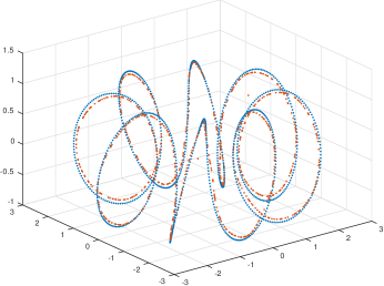
Figure 11: Helix data set and density ridge projection. True data set without noise shown in blue and density ridge projection with lowest mean square error in red.

The next example shows a two dimensional plane bent into a half-cylinder shape. A uniform sample is drawn from the surface and zero mean gaussian noise is added, see figure 12(a). We show the result using different kernel sizes in figure 12(b), to visually confirm that the bias of the density ridge estimate increases as the kernel size increases. the largest kernel size gives the most smooth result, but the curvature of the half-cylinder is reduced. for the smaller kernel sizes we see that the ridge estimator is closer to the true manifold, but that many of the noisy points become local maxima and is not projected to the density ridge.

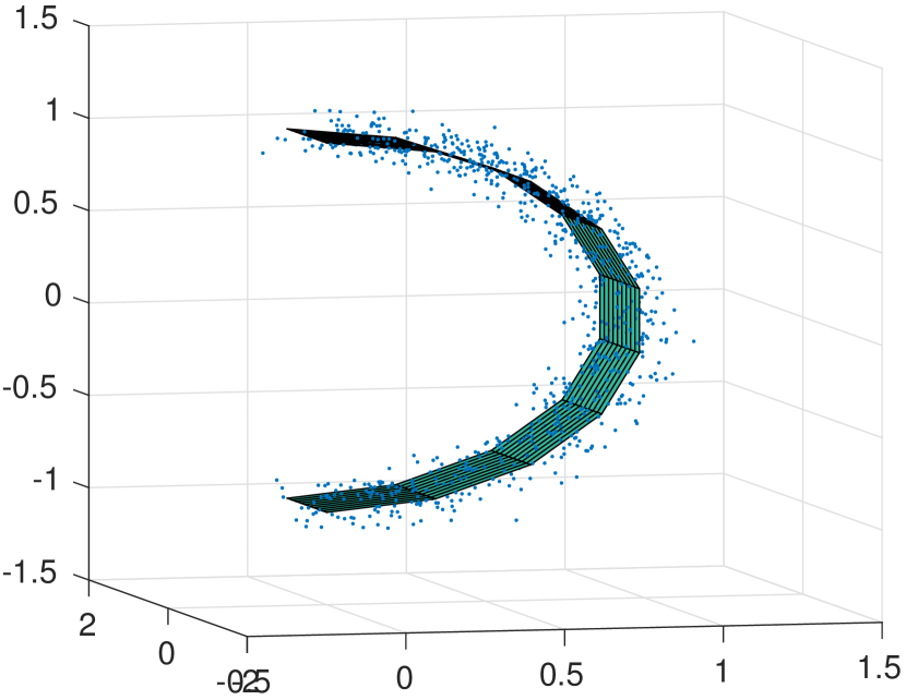
(a) Half cylinder manifold(solid) sampled with noise(dots).

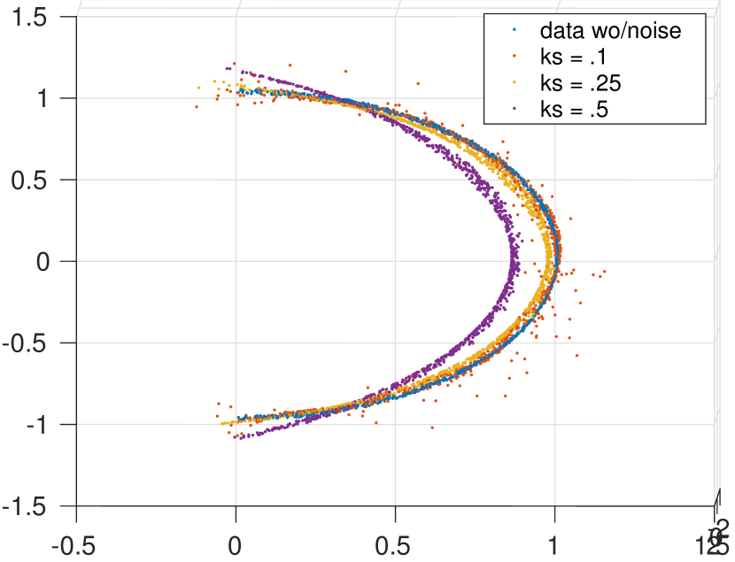
(b) Estimated density ridge of half cylinder manifold. The ridge is shown for a range of kernel sizes to illustrate the bias introduced. The true manifold is shown in blue dots.

Figure 12: Noisy half-cylinder manifold estimated at different kernel sizes.

7.2 influence of kernel size

The choice of kernel bandwidth is very important in estimating density ridges, and can have great influence on the results.

To illustrate the influence of kernel size we sample uniformly from a sphere, $\mathbb{s}^{2}$, and add different levels of $n(0,\varepsilon_{i})$ noise. In table 1 the mean squared error between the true manifold and the ridge for the different kernel bandwidths and levels of noise is shown.

Table 1: Mean squared error of ridge estimates for different levels of noise($\varepsilon$) and kernel sizes($\sigma^{2}$).

$\sigma^{2}$ \$\varepsilon$	.05	.1
.1	0.0103	0.0973
.25	0.0079	0.0909
.5	0.0140	0.0969
.7	0.0347	0.1267
1	0.1256	0.1901
2	0.2046	0.2738

In this concrete example we see that a kernel size of approximately $0.25$ gives the density ridge that is closest to the underlying manifold. We also see that even in the low noise case, the mean squared error of the estimates deteriorates quickly due to bias in the estimations.

In the rest of the paper – unless otherwise noted – we have used a heuristic choice of the average distance to the 12th nearest neighbor as kernel size for the gaussian kernel (Myhre and Jenssen, 2012).

7.3 Manifold unwrapping

In this section we show results on unwrapping one-dimensional manifolds with noisy embeddings in higher dimensions – $\mathbb{R}^{d}$, $d\geq 1$. We start with the full unimodal example from section 4. In figure 13(a) we see the data set, its two orthogonal density ridges and the contours of the density.

(a) Nonlinear unimodal data set with density ridges shown in red and blue and the equiprobable contour lines of the kernel density estimate shown.

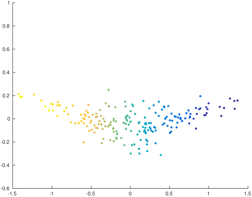
(b) Unwrapped version of the nonlinear distribution.

Figure 13: One crescent moon data set. Original and unwrapped version.

The same data set can be seen in figure 13(a). After applying the local density ridge unwrapping algorithm, we get the results shown in figure 13(b). We see that by calculating distances along the underlying structure we reveal the distribution along the intrinsic geometry. In this case a gaussian kernel was used with a manually chosen kernel bandwidth of $0.5$. If we inspect closer we see that there is a slight bias in the first ridge, show in red, in figure 13(a). This bias can also be seen in the unwrapped results, as they show a very downscaled version of the original nonlinearity. This could be avoided by either choosing a smaller kernel size, but risking more variance in the ridge and thus less accurate unwrapped coordinates or by using a varibable kernel density estimator (Wand and Jones, 1994; Bas, 2011).

7.4 Density ridge translation

To illustrate the density ridge translation algorithm we use a spiral shaped data set with gaussian noise as shown in figure 14. The underlying manifold is parameterized as $\bigl{(}\begin{smallmatrix}\mathbf{x}_{1}\\ \mathbf{x}_{2}\\ \end{smallmatrix}\bigr{)}=\bigl{(}\begin{smallmatrix}r\cos\theta\\ r\sin\theta\end{smallmatrix}\bigr{)}$ , with $\theta=\left[0,2\pi\right]$ and $r=\left[0,2\right]$. The $\theta$ parameter is indicated by the color coding from dark blue to light yellow. The two local orthogonal density ridges are shown in figure 15(a) and we note that there are two separate local maxima. This will give rise to two different local charts by algorithm 1. In figure 15(b) we see the results after applying the density ridge translation algorithm on the charts.

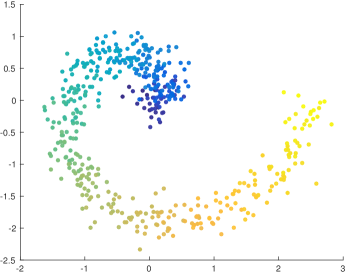
Figure 14: Spiral shaped data set with gaussian noise. Color coding indicates data point order in parameterization.

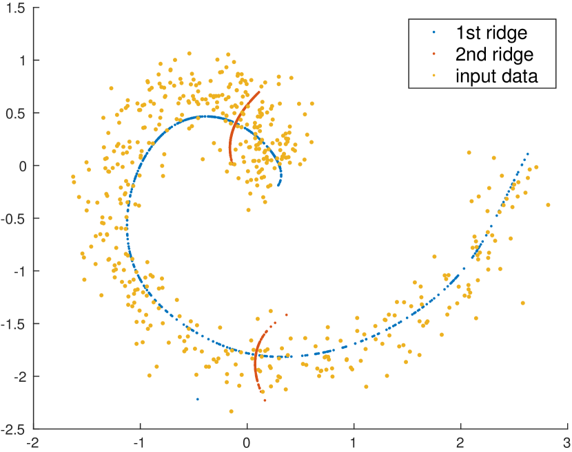
(a) Spiral shaped dataset with two orthogonal density ridges.

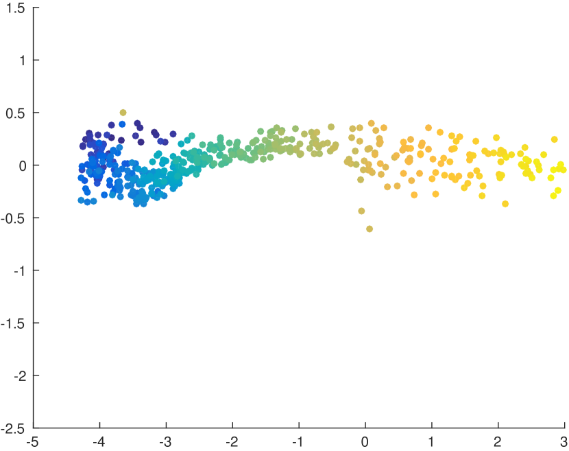
(b) Spiral shaped data set after the density ridge translation algorithm.

Figure 15: Spiral data set with density ridges and unwrapped version.

It is clear that the new unwrapped representation of the data follows the color coding directly, and the total horizontal variation from $-4$ to $3$ fits nicely with a centered version – $\left[-\pi,\pi\right]$ – of the original parameterization from $0$ to $2\pi$. In the top left of the unwrapped data structure we see some distortion with respect to the parameterization/color coding of the original data. This is most probably again due to bias in the density ridge estimation. The nonlinearity of the innermost part of the spiral is most likely on a smaller scale than the kernel bandwidth is able to capture, resulting in a density ridge that is straighter than it should be and thus the projections will be less accurate.

7.5 pca preprocessing and local density ridge unwrapping

In this section we present results on real data sets preprocessed by principal component analysis (Jolliffe, 2002).

7.5.1 Subset of mnist handwritten digits

In this experiment we use a subset of the mnist handwritten images. We preprocess the data by projecting the data to the first three principal components. We use images of the number one – $1$ – in this experiment, since it is very susceptible to geometric variations like rotations, translations and also more nonlinear deformations due to its simple shape.

The data projected to the top three principal components is shown in figure 16(a). We clearly see that the data follows a nonlinear submanifold and that the variation of the images varies along a low dimensional surface. To test our framework, we project the data to the two-dimensional density ridge, and find the local modes by following the gradient.

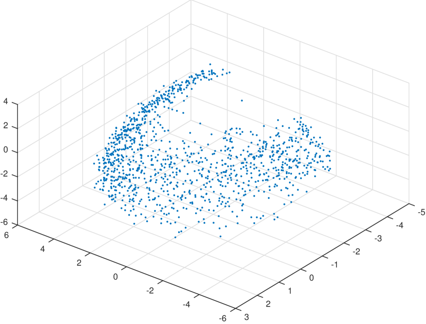
(a) The ones of the mnist data set projected to top three principal curves.

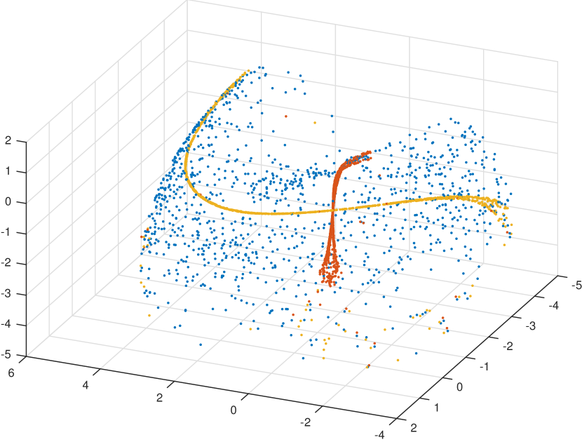
(b) Mnist handwritten digits image data projected to the top three principal components. The red and yellow curves shows the two one-dimensional density ridges of the projected dataset.

Figure 16: mnist-ones projected to three dimensions.

If we use a large kernel bandwidth we introduce some bias in the density ridge estimate seen e.g. in the splitting of the curves near the boundary of the manifold, but at the same time we get two global principal curves that cover the entire projected data set, shown in figure 16(b) such that there is no need to translate charts together and we can directly get a global unwrapping. In figure 17 we see the results of applying the local density ridge unwrapping algorithm (algorithm 1).

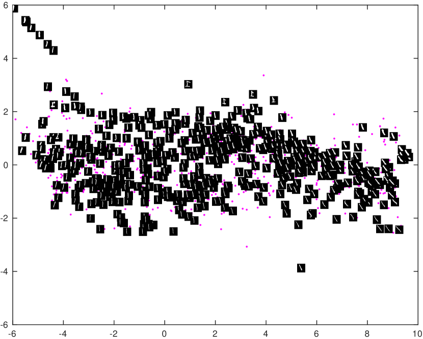
Figure 17: mnist data set – as shown in figure 16(b) – unwrapped by using algorithm 1.

In figure 17 we see the unwrapped mnist digits with a selection of random images of the actual digits on top. We see that the coordinates represents a clear structure in the data – a straight up version of the digit around the origin and different, but symmetric variations along the two axes. The horizontal axis represents the orientation of the digits, while the vertical axis represesents thickness of the digits. in section 7.9 we compare our results with other known manifold learning algorithms. as a final remark in this setting we note that the use of pca preprocessing is a linear projection such that the geometric properties of the data should not be influenced by the transformation. Ideally pca would remove all ambient space except $\mathbb{R}^{d+1}$ such that the codimension Is one.

7.5.2 Frey faces

In this section we test the local density ridge unwrapping on the frey faces data set. For visualization purposes we reduce the dimension of the data set down to two by pca – shown in figure 18(a). We clearly see an underlying curved structure.

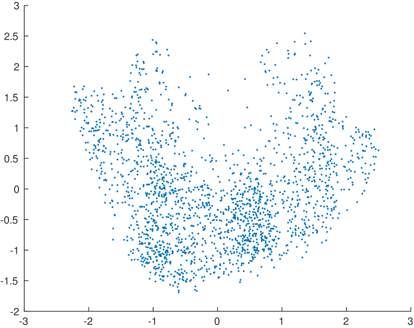
(a) Frey face images after reduction to two dimensions by principal component analysis.

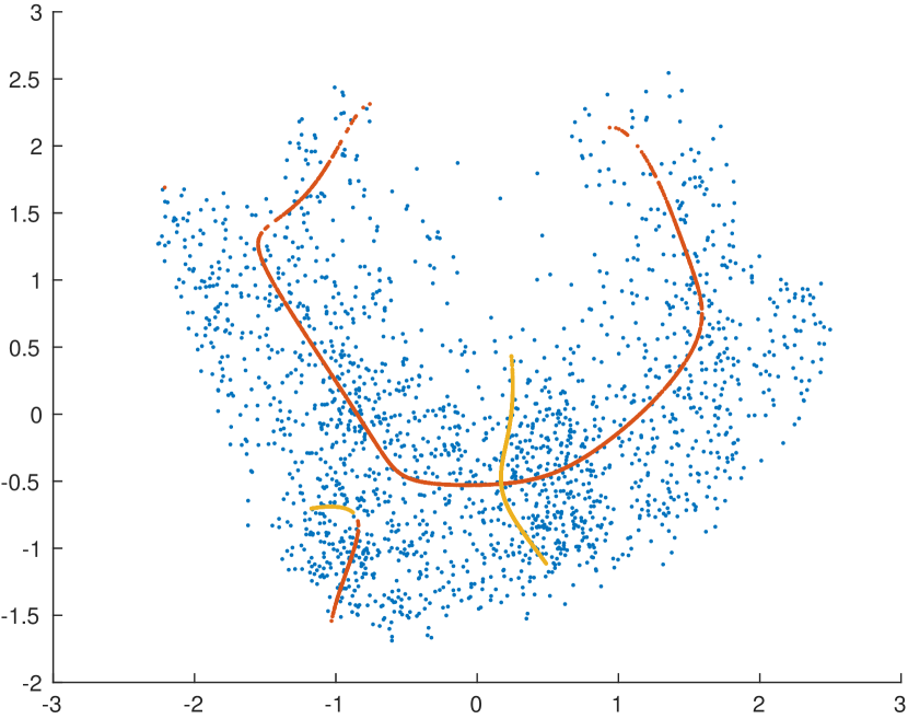
(b) Frey faces image after pca with the first and second one-dimensional density ridges as found by equation (1) shown in red and orange respectively.

Figure 18: frey faces reduced to two dimensions by pca.

The curved structure has seemingly large orthogonal variance so we project to both of the two available one-dimensional density ridges. The result can be seen in figure 18(b). The first density ridge/principal curve, according to the ordering of the eigenvalues of the local hessian, is shown in red. It captures well the underlying nonlinearity. The second ridge, shown in orange, fits well with the orthogonal variation along the underlying nonlinearity. We also have to note the disconnected ridges in the bottom left part of the data set. This is probably due to a separate curvilinear structure in the data. We could alleviate this by choosing a larger kernel size to increase the smoothness of the ridge, but then there would be a risk of smoothing away the nonlinear curved structure of the data. We proceed with the chosen kernel size and note that this case cannot be described by a single one-dimensional manifold.

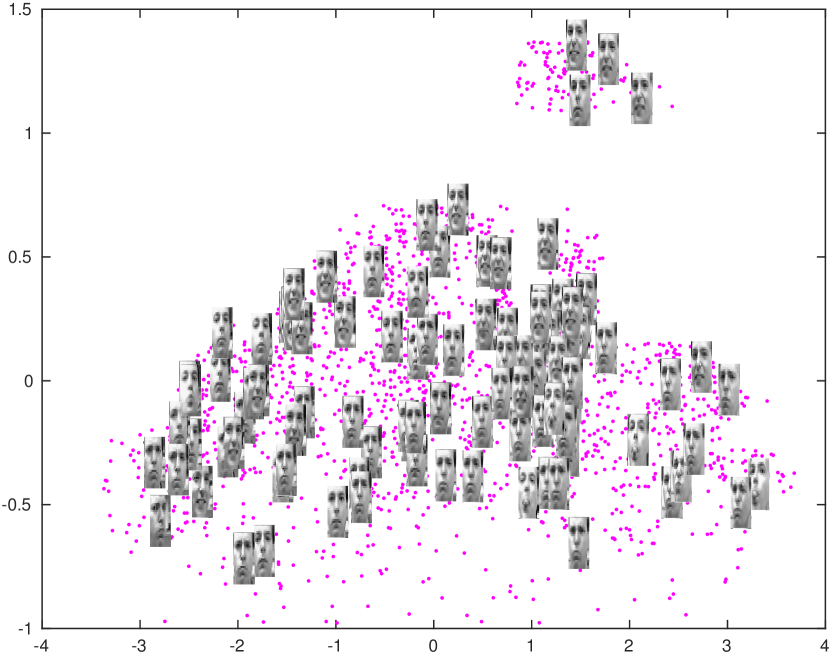
Figure 19: Unwrapped version of the frey faces. A random selection of actual face images shown on top of the unwrapped coordinates for illustration of structure.

In figure 19 we see the results of the local density ridge unwrapping algorithm. A random selection of 100 of the original input images are displayed on top of the unwrapped coordinates. We see that the main horizontal direction, exhibiting the largest variance, captures the left-right orientation of the faces. In figure 20 each row shows the largest negative, origin and largest positive coordinate of each of the two coordinates of the unwrapping respectively. We again see that the first ridge - top row - corresponds to the left-right orientation of the faces. The second ridge is harder to interpret, but we note that the orientation of the face is looking straight ahead in all bottom three images in figure 20, which fits well with the second coordinate being orthogonal to the horizontal direction represented by the first coordinate.

The disconnected ridges results in the region in the top right corner. The analysis and discussion of these cases are left for future research.

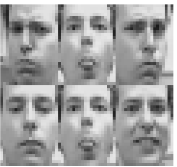
Figure 20: Top row: largest, orgin and smallest first unwrapped coordinate. Bottom: largest, origin and smallest second unwrapped coordinate.

7.6 $d$-dimensional ridges

In this section we present some applications of our non-parametric $d$-dimensional framework. Inspired by dollár et al.  (Dollár et al., 2007), we can perform several different operations once each point that lies on the manifold has been equipped with a tangent space - spanned by the hessian eigenvectors. Most important in this setting are calculating geodesics as in equation (9), and out-of-sample projections that are faster than projections by solving differential equations.

We include two examples: the first example shows out of sample projections by projecting so point to the closest local tangent space. The second example shows smooth geodesics found by the alternating least squares algorithm presented in section 6.2.

In figure 21 we see a synthetic hemisphere sampled uniformly with $n(0,.3i)$ noise added.

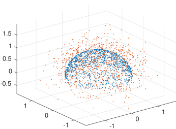
Figure 21: Data sampled from a hemisphere with(red) and without noise(blue). The noise level is $n(0,.3i)$.

In figure 22 we see the points projected to the closest tangent space of the density ridge by equation 10.

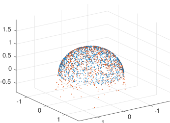
Figure 22: The hemisphere data projected to the local tangent space using the method from dollar

It is obvious that the out of sample projections are working as expected, but we also see that when samples are so noisy that they cannot be orthogonally projected to the manifold - in this case they are not directly above the hemisphere - they are projected to the tangent space of the boundary of the manifold, and the structure is thus lost. In this case the flat tangent spaces at the boundary gives the appearance of projecting to a cylinder below the hemisphere. Suggestions and solutions to this problem is left to future research.

7.7 Isometric unwrapping

In the case where the intrinsic manifold has zero gaussian curvature it can be unfolded isometrically by the algorithms from section 6. We start with the ‘swissroll’ example, a two dimensional surface of zero gaussian curvature distorted by a nonlinear function and $n(0,\sigma^{2})$-noise. This is a popular dataset/example to illustrate manifold learning algorithms. It is useful because it represents a strong non-linear structure, but at the same time it is a simple surface without gaussian curvature such that it can in fact be represented by a single coordinate chart. After projecting to the ridge and running the algorithms, we get the result of unwrapping shown in figure 23.

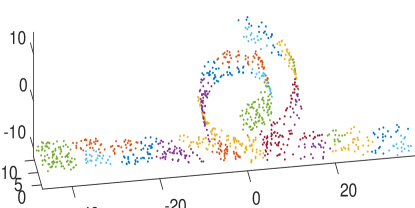
Figure 23: Swissroll dataset with unwrapped coordinates shown in the tangent space of the reference mode.

The color coding illustrates the local basins of attraction. In the unwrapped version - shown in the tangent space of one of the modes - we clearly see that the ordering of the local charts is preserved.

7.8 mnist autoencoder

We end this section with an example of a real data set where multiple $d$-dimensional charts emerge such that the isometric unwrapping algorithm, algorithms 3 and 4, has to be applied. Again we use the mnist one digits, but this time we reduce the dimension to three by using a deep autoencoder - as given in (van der Maaten et al., 2009).

In figure 24 we see both the data set and the data projected to the two-dimensional density ridge. The underlying ridge fits the data well, and we see that there are several local charts involved, indicated by the color coding.

After running the isometric density ridge unwrapping scheme we get the results shown with a random selection of digits overlaid in figure 25. We again se a clear structure in the data with the ones rotating/changing orientation along the horizontal axis. The structure in the other mnist-ones example, where the ones changed from thicker to thinner along the vertical axis is not as strong in this example.

Figure 24: Mnist one digits after reducing dimension to three by using an autoencoder (small red dots) and the two-dimensional density ridge. The color coding of the ridge indicates the local charts/attraction basins found.

Figure 25: Isometric unwrapping on mnist ones after reducing dimension to three by using an autoencoder.

7.9 Comparison with other unwrapping algorithms

Finally we compare our algorithm with isomap (Tenenbaum et al., 2000), local linear embedding (Roweis and Saul, 2000), local tangent space alignment (Zhang and Zha, 2004) and maximum variance unfolding (Weinberger and Saul, 2006). We use a synthetic data set consisting of a two-dimensional surface embedded in $\mathbb{R}^{3}$ with additive/convolutional gaussian noise in addition to the mnist-ones used previously.

For the mnist-ones, we use our isometric unwrapping with a slightly smaller kernel size than the previous example - recall that the previous example a large kernel size was used to obtain one-dimensional ridges that cover the entire manifold. This leads to several local modes, and thus several charts over the manifold such that algorithms 3 and 4 have to be used. The result is shown in figure 27. The other algorithms - isomap, lle, ltsa and mvu - all have a $k$-nearest-neighbor parameter that has to be set so we run them with different values of $k=\begin{bmatrix}5,12,20,50,100\end{bmatrix}$ and select the most visually meaningful results, shown in figure 26. We note that the ltsa had problems with finding the eigenvalue/eigenvectors such that the $k$ values had to be set much higher - $k=\begin{bmatrix}150,300\end{bmatrix}$.

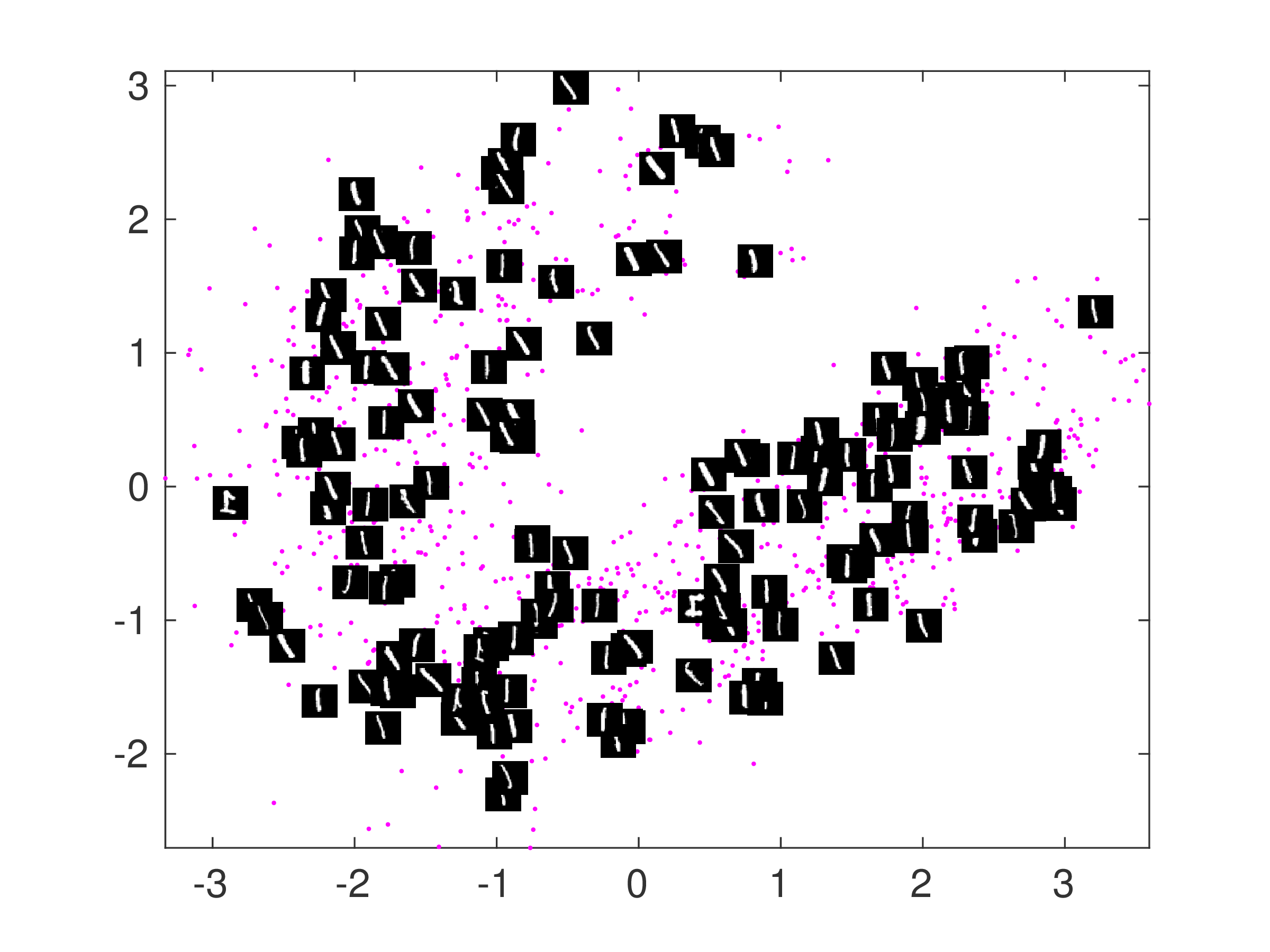
(a) Maximum variance unfolding. $k=12$

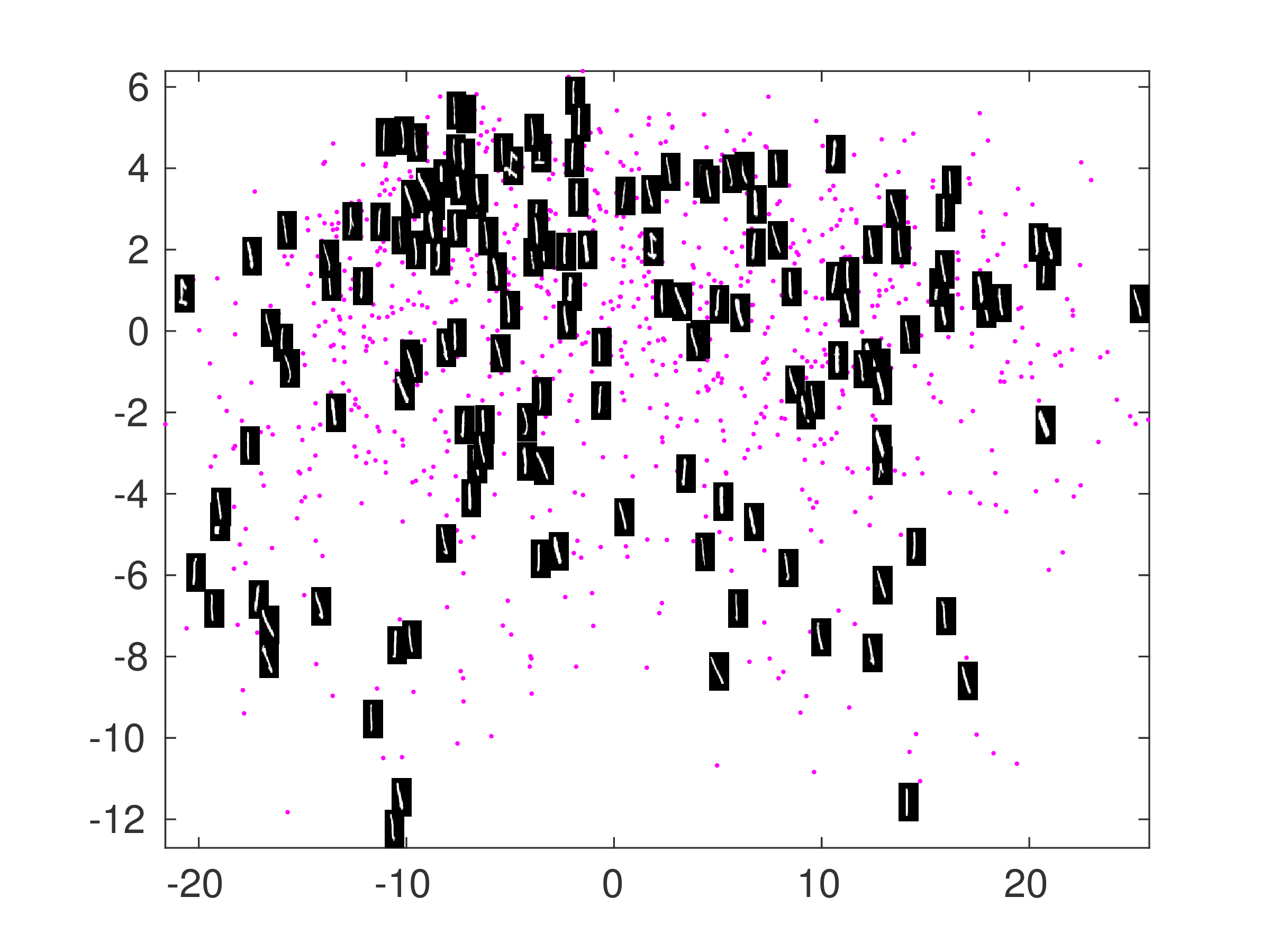
(b) Isomap. $k=20$

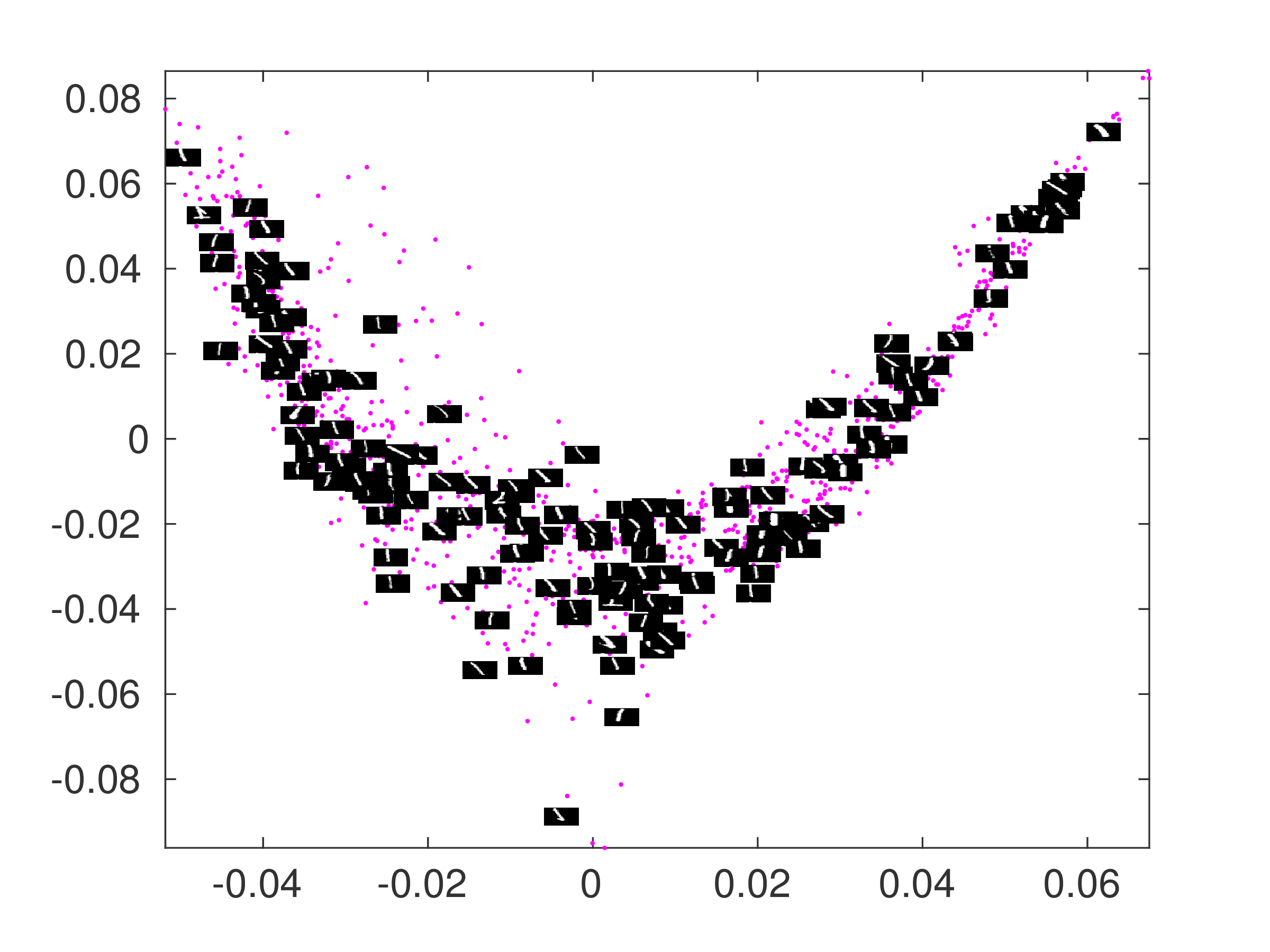
(c) Local linear embedding. $k=20$.

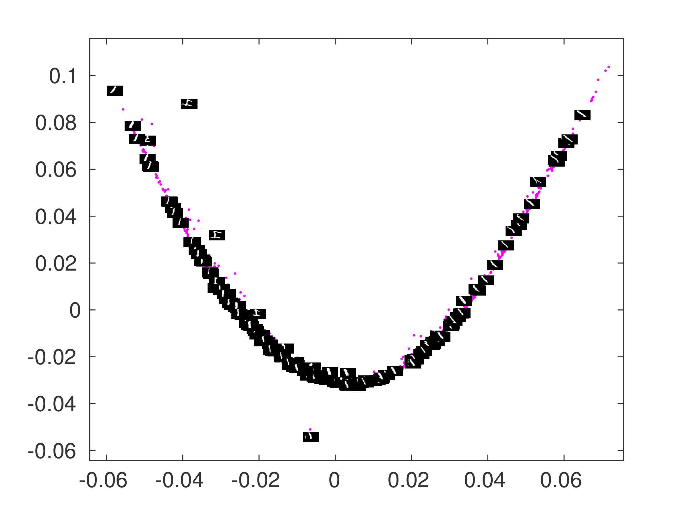
(d) Local tangent space alignment. $k=150$

Figure 26: mnist-ones dataset tested on several benchmark manifold learning algorithms.

Local tangent space alignment, figure 26(d) shows a similar structure to the density ridge unwrapped result that follows the orientation of the digit, but the structure is compressed to a curve and the structure orthogonal to the curve is lost. There is also no apparent unwrapping, the manifold is still curved. The same goes for the local linear embedding result, figure 26(c), no apparent unwrapping. Also, looking at the images overlaid over the data, there does not seem to be the same smooth consistent structure as in the density ridge unwrapped version. Isomap, figure 26(b) has unwrapped the manifold, but the structures seen in the overlaid images does not seem to follow specific patterns. Finally, maximum variance unfolding in figure 26(a) has also failed in unwrapping the noisy cylinder shape, we also note that the orientation of the numbers is not preserved properly.

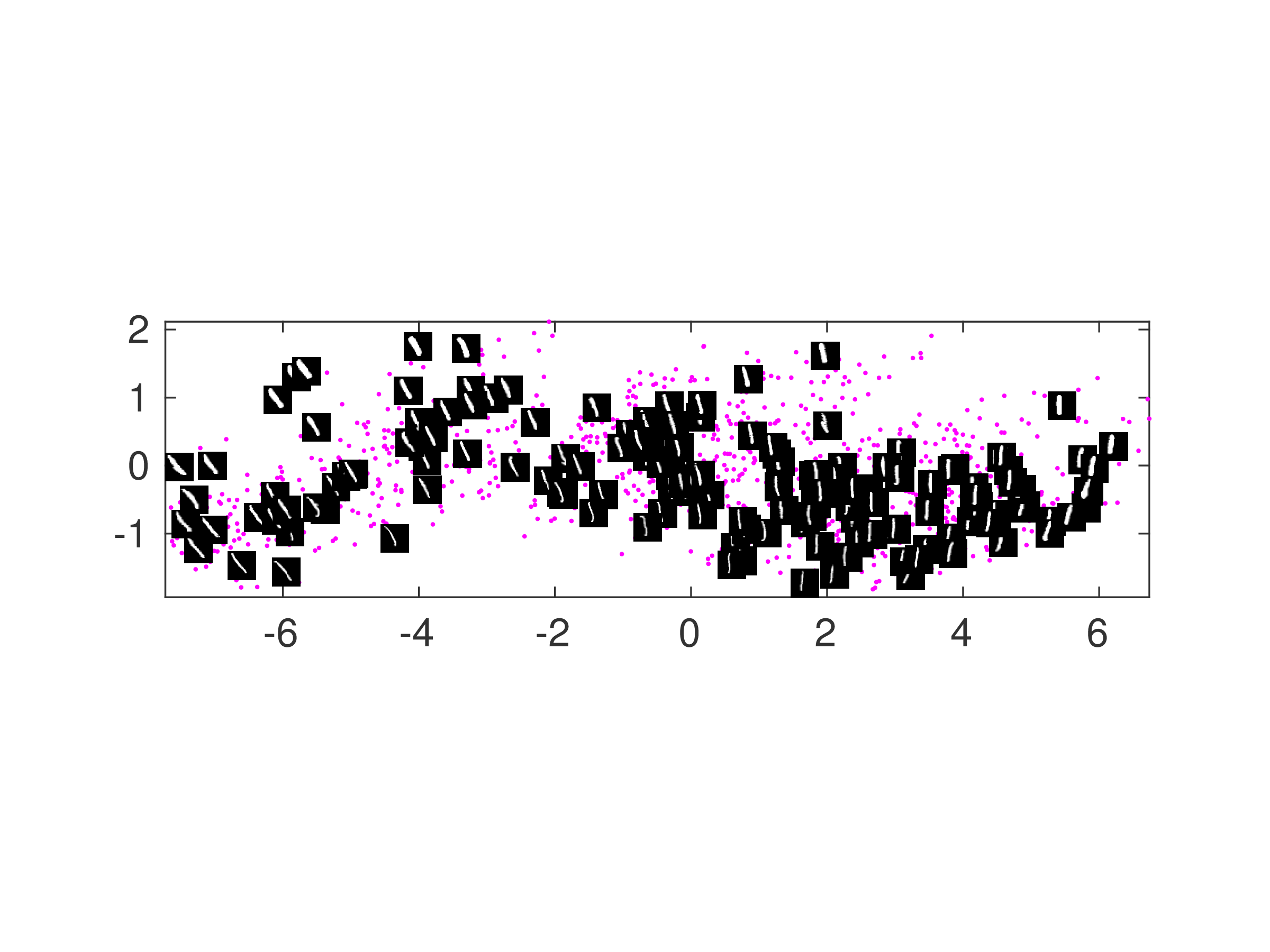
Figure 27: Density ridge unwrapping on mnist-ones.

Finally we do the same comparison on a synthetic data set with a high level of noise to indicate that our algorithm can handle noisy situations. The data set with and without noise and the density ridge unwrapped version projected to the tangent space of the reference mode is shown in figure 28. We see that even with a quite high level of noise the density ridge unwrapping gives meaningful results. In figure 29 we see the data processed to two-dimensions by isomap, lle, mvu, ltsa, laplacian eigenmaps and density ridge unwrapping. The original parameterization is shown in red dots, and the unwrapped coordinates from the different algorithms are shown with the same color coding as in figure 28. All result were obtained with neighborhood parameter $k=12$ and the results as well as the parameterization have been normalized and centered.

Looking at the figures we see that isomap is the closest to ours, but it is not able to capture the manifold without retaining the noise. The other four algorithms, laplacian eigenmaps, local linear embedding, maximum variance unfolding and local tangent space aligment all fail to unfold the underlying manifold and the results are accordingly hard to comment on. We tried different parameters for all algorithms, but all failed to give reasonable results, except isomap and our algorithms, that is why we chose to show only the results of the default parameter $k=12$.

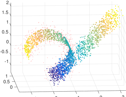
Figure 28: Dataset with(red dots) and without(colored dots) noise. The result of our algorithm projected to the tangent space of a reference mode shown in similar colors as the data without noise.

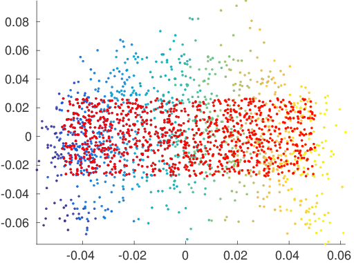
(a) Isomap $k=12$.

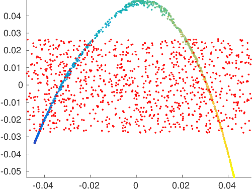
(b) Laplacian eigenmaps $k=12$.

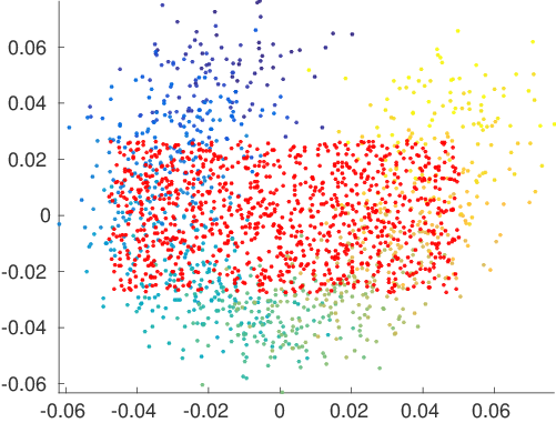
(c) Local linear embedding $k=12$.

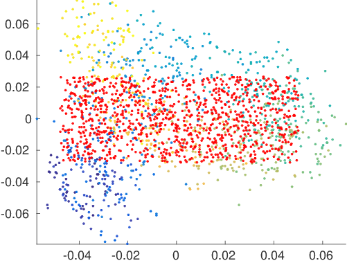
(d) Maximum variance unfolding $k=12$.

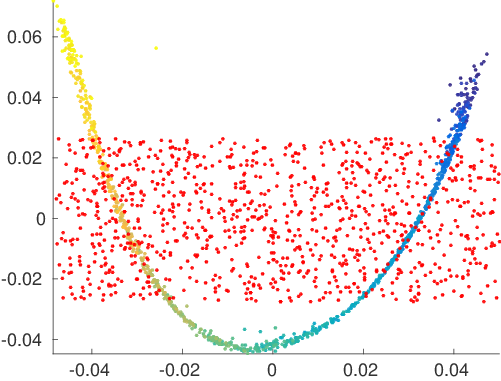
(e) Local tangent space alignment $k=12$.

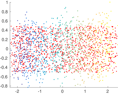
(f) Density ridge unwrapping.

Figure 29: Uncovering the underlying parameterization of figure 28 using various manifold unwrapping algorithms.

8 Conclusion and future work

In this paper we have shown that density ridges of a kernel density estimate can be used to unwrap manifolds. We have presented a geometrically intuitive algorithm for unwrapping one-dimensional manifolds embedded in euclidean space based on gradient flow. We have extended this algorithm to higher dimensional manifolds, replacing coordinates calculated via integral curves to local linear projections. promising results and illustrations have been shown on both synthetic and real data sets that match the geometric intuition of unfolding.

We conclude this paper with a short section on possible extensions and directions of further research.

8.1 Future research

The work presented in this paper contains suggestions on how to learn linear coordinate systems on non-linear data distributions that can be represented by principal curves or surfaces (density ridges). The perhaps most obvious lines of further research are related to the properties of the underlying manifold and the estimate of the manifold surrogate which relies on the kernel density estimate of the distribution of points on the manifold.

Regarding the properties of the underlyng manifold theoretical results should be established related to upper bounds on the curvature, boundary effects and smoothness properties in higher dimension. The online appendix for the convergence proofs of the isomap algorithm could be applied here (Tenenbaum et al., 2000).

Furthermore, the properties of the underlying manifold directly influences the density ridge estimate. Especially the choice of kernel size and how it influences the relationship between curvature, bias and smoothness of the density ridge estimate should be established theoretically. Also the properties of the kernel density estimate is known to deteriorate when the dimension increases since the distance distribution of a point set converges to the mean distance in higher dimensions. An upper bound on dimensions where the gradient flow of a kernel density estimate holds could be established and used in our setting.

Recently chacon and duong, Chacón et al. (2013) suggested kernel size estimators that yield different sizes for kernel density its gradient and its hessian. These could be implemented in our setting, perhaps increasing accuracy in density ridge estimations.

Aknowledgements

This work was partially funded by the research council of norway over fripro grant no. 239844 on developing the next generation learning machines (rj).

A Approximate parallel transport

In this section we present the algorithm for approximate parallel transport in the $d$-dimensional setting. Let $\hat{R}_{i}$ be the points on the ridge estimate that lies in the basin of attraction of mode $\mathbf{m}_{i}$ and $C_{i}$ the local coordinates of $\hat{R}_{i}$, $C_{i}=Q_{||}(\mathbf{m}_{i})Q_{||}(\mathbf{m}_{i})^{T}\hat{R}_{i}$. Let $\boldsymbol{\gamma}$ be the vector containing the points of the approximate geodesic from $\gamma_{0}=\mathbf{m}_{i}$ to $\gamma_{n}=\mathbf{m}_{j}$ as found by (9). The approximate parallel transport is performed by translating the local coordinates $C_{i}$ along the finite difference tangent vectors of the approximate geodesic. At each step of the translation the points are projected/rotated to the local tangent space by $Q_{\parallel}(\gamma_{t})Q_{\parallel}(\gamma_{t})^{T}$. This is to ensure that the local coordinates stay in the tangent space all the way along the geodesic towards the target mode $\mathbf{m}_{j}$. The algorithm for approximate parallel transport is summarized in Algorithm 3.

Algorithm 3 Approximate parallel transport from $\mathbf{m}_{i}$ to $\mathbf{m}_{j}$

0:  $C_{i}$ and $\boldsymbol{\gamma}=\left[\gamma_{t}\right]_{t=1}^{n}$.

1:  Calculate $Q_{||}(\gamma_{t})$ for $t=[1,\cdots,n]$.

2:  Initialize $C_{i}^{{}^{\prime}}=C_{i}$.

3:  for $t=[2,\cdots,n]$ do

4:     

$$C_{i}^{{}^{\prime\prime}}=Q_{||}(\gamma_{t})Q_{||}(\gamma_{t})^{T}\left(C_{i}^{{}^{\prime}}+(\gamma_{t}-\gamma_{t-1})\right)$$ (11)

5:     $C_{i}^{{}^{\prime}}=C_{i}^{{}^{\prime\prime}}$

6:  end for

6:  Local coordinates $C_{i}^{{}^{\prime}}$ transported from $\mathbf{m}_{i}$ to $\mathbf{m}_{j}$ along the manifold.

B Algorithm for unwrapping transported coordinates

Given a framework for approximate parallel transport, we can unwrap isometric manifolds. This is done by first transporting all local linear attraction basin approximations (charts) to a reference mode. Then each chart is iteratively translated back along the geodesic it came from whilst at the same time projecting each step down to the dimension of the tangent space along the same geodesic. This will give an unfolded version of the manifold where all charts lie in the dimension of the tangent space of the manifold centered on the reference mode.

Let $\boldsymbol{\nu}$ be the vector $\boldsymbol{\gamma}$ in reversed order. Since $\boldsymbol{\nu}$ lies approximately on the manifold the finite difference tangent vectors $\delta\nu=\nu_{t+1}-\nu_{t}$ will also lie on the manifold. So by pushing the coordinates along the geodesic and at the same time projecting to the intrinsic dimension of the manifold, we get a direct unfolding. The complete algorithm is presented in Algorithm 4.

Consider standing on the north pole of the earth and taking a step in some direction along the surface of the earth. Following the algorithm, one would take a step in the chosen direction and project the vector pointing from the north pole to the destination of the step to the tangent space of the north pole. This would yield a two-dimensional step in the tangent space of the north pole. Then the procedure is repeated from the next position; take a step and then project to the tangent space of the origin. The tangent space will still be two-dimensional, but the orientation might have changed slightly, so that we need to compensate for the change of basis from tangent space to tangent space.

In this manner one will get a two-dimensional representation of the path walked, e. g. walking from the north pole to the south pole along a great circle would yield a straight line in the unfolded coordinates. Note the similarity to stereographic projection coordinates. Of course this example is in effect not relevant since the earth is close to a sphere which cannot be unfolded isometrically, but the analogies to the algorithm still holds.

Algorithm 4 Isometric unfolding

0:  Local coordinates transported to a reference mode $C=\{C_{i}^{{}^{\prime}}\}_{i=1}^{m-1}$ and the reversed geodesic from reference mode to all other modes, $\boldsymbol{\nu}_{i}$.

1:  Choose a basis $E_{i}$ for the tangent space of a point on the reversed geodesic $\nu_{t}$, $T_{\nu_{t}}M$:

$$E_{i}=\begin{bmatrix}\Delta\nu_{t}&\text{null}\left(\begin{bmatrix}\Delta\nu_{t}&Q_{\perp}\left(\nu_{t}\right)\end{bmatrix}\right)\end{bmatrix}^{T}.$$

2:  for all Translated charts $C_{i}^{{}^{\prime}}$ do

3:     for $t=[2,\cdots,n]$, $n$ is the number of steps in $\boldsymbol{\nu}_{i}$ do

4:        Choose the translation direction as being along $\nu_{t}$ such that the step along the geodesic will be $\xi=[\|\nu^{\prime}_{t}\|,\;\mathbf{0}]^{T}$, $\xi\in\mathbb{R}^{D}$, $\mathbf{0}\in\mathbb{R}^{D-1}$.

5:        Make sure that the basis stays consistent: $B=BE_{t}^{T}E_{t+1}$, initialized as $B=E_{1}$.

6:        Project the translation to the tangent space, $U_{i}=Q_{\parallel}(\nu_{t})Q_{\parallel}(\nu_{t})^{T}\left(C^{{}^{\prime}}_{i}+B\xi_{t}\right)$

7:     end for

8:  end for

8:  Unwrapped manifold consisting of all unwrapped charts $\widehat{M}=\bigcup_{i=1}^{m}U_{i}$.

References

- Arias-Castro et al. (2013) Ery Arias-Castro, David Mason, and Bruno Pelletier. On the estimation of the gradient lines of a density and the consistency of the mean-shift algorithm. Unpublished manuscript, 2013.
- Banfield and Raftery (1992) Jeffrey D Banfield and Adrian E Raftery. Ice floe identification in satellite images using mathematical morphology and clustering about principal curves. Journal of the American Statistical Association, 87(417):7–16, 1992.
- (3) Margherita Barile and Eric W. Weisstein. T2-space. URL http://mathworld.wolfram.com/T2-Space.html. Visited on 25/02/15.
- Bas (2011) Erhan Bas. Extracting structural information on manifolds from high dimensional data and connectivity analysis of curvilinear structures in 3D biomedical images. PhD thesis, NORTHEASTERN UNIVERSITY, 2011.
- Brun et al. (2005) Anders Brun, Carl-Fredrik Westin, Magnus Herberthson, and Hans Knutsson. Fast manifold learning based on riemannian normal coordinates. In Image Analysis, pages 920–929. Springer, 2005.
- Burges (2009) Christopher JC Burges. Dimension reduction: A guided tour. Machine Learning, 2(4):275–365, 2009.
- Chacón et al. (2013) José E Chacón, Tarn Duong, et al. Data-driven density derivative estimation, with applications to nonparametric clustering and bump hunting. Electronic Journal of Statistics, 7:499–532, 2013.
- Chang and Ghosh (1998) Kyu-Yu Chang and Joydeep Ghosh. Principal curve classifier-a nonlinear approach to pattern classification. In Neural Networks Proceedings, 1998. IEEE World Congress on Computational Intelligence. The 1998 IEEE International Joint Conference on, volume 1, pages 695–700. IEEE, 1998.
- Chen et al. (2014a) Yen-Chi Chen, Christopher R Genovese, and Larry Wasserman. Asymptotic theory for density ridges. arXiv preprint arXiv:1406.5663, 2014a.
- Chen et al. (2014b) Yen-Chi Chen, Christopher R Genovese, and Larry Wasserman. Generalized mode and ridge estimation. arXiv preprint arXiv:1406.1803, 2014b.
- Chen et al. (2014c) Yen-chi Chen, Larry Wasserman, and Christopher R. Genovese. SOLUTION MANIFOLDS IN STATISTICS By Yen-Chi Chen, Christopher R. Genovese and Larry Wasserman Carnegie Mellon University June 29, 2014. pages 1–33, 2014c.
- Comaniciu and Meer (2002) Dorin Comaniciu and Peter Meer. Mean shift: A robust approach toward feature space analysis. Pattern Analysis and Machine Intelligence, IEEE Transactions on, 24(5):603–619, 2002.
- Dijkstra (1959) Edsger W Dijkstra. A note on two problems in connexion with graphs. Numerische mathematik, 1(1):269–271, 1959.
- Dollár et al. (2007) Piotr Dollár, Vincent Rabaud, and Serge Belongie. Non-isometric manifold learning: Analysis and an algorithm. In Proceedings of the 24th international conference on Machine learning, pages 241–248. ACM, 2007.
- Einbeck et al. (2005) Jochen Einbeck, Gerhard Tutz, and Ludger Evers. Local principal curves. (1992):301–313, 2005.
- Fehlberg (1969) Erwin Fehlberg. Low-order classical Runge-Kutta formulas with stepsize control and their application to some heat transfer problems. 1969.
- Freifeld et al. (2014) Oren Freifeld, Soren Hauberg, and Michael J Black. Model transport: Towards scalable transfer learning on manifolds. In Computer Vision and Pattern Recognition (CVPR), 2014 IEEE Conference on, pages 1378–1385. IEEE, 2014.
- Genovese et al. (2009) Christopher R Genovese, Marco Perone-Pacifico, Isabella Verdinelli, Larry Wasserman, et al. On the path density of a gradient field. The Annals of Statistics, 37(6A):3236–3271, 2009.
- Genovese et al. (2012) Christopher R Genovese, Marco Perone-Pacifico, Isabella Verdinelli, and Larry Wasserman. The geometry of nonparametric filament estimation. Journal of the American Statistical Association, 107(498):788–799, 2012.
- Genovese et al. (2014) Christopher R. Genovese, Marco Perone-Pacifico, Isabella Verdinelli, and Larry Wasserman. Nonparametric ridge estimation. The Annals of Statistics, 42(4):1511–1545, August 2014. ISSN 0090-5364. doi: 10.1214/14-AOS1218. URL http://projecteuclid.org/euclid.aos/1407420007.
- Gerber (2013) Samuel Gerber. Regularization-Free Principal Curve Estimation. 14:1285–1302, 2013.
- Gerber and Whitaker (2013) Samuel Gerber and Ross Whitaker. Regularization-free principal curve estimation. The Journal of Machine Learning Research, 14(1):1285–1302, 2013.
- Hastie and Stuetzle (1989) Trevor Hastie and Werner Stuetzle. Principal curves. Journal of the American Statistical Association, 84(406):502–516, 1989.
- Heckbert (1990) Paul S Heckbert. A seed fill algorithm. In Graphics gems, pages 275–277. Academic Press Professional, Inc., 1990.
- Hein and Maier (2006) Matthias Hein and Markus Maier. Manifold denoising. In Advances in neural information processing systems, pages 561–568, 2006.
- Jolliffe (2002) Ian Jolliffe. Principal component analysis. Wiley Online Library, 2002.
- Kégl et al. (2000) Balázs Kégl, Adam Krzyzak, Tamás Linder, and Kenneth Zeger. Learning and design of principal curves. Pattern Analysis and Machine Intelligence, IEEE Transactions on, 22(3):281–297, 2000.
- Krzy (2002) Adam Krzy. Piecewise linear skeletonization using principal curves ∗. 7, 2002.
- LeCun et al. (1998) Yann LeCun, Léon Bottou, Yoshua Bengio, and Patrick Haffner. Gradient-based learning applied to document recognition. Proceedings of the IEEE, 86(11):2278–2324, 1998.
- Lee (1997) John M Lee. Riemannian manifolds: an introduction to curvature, volume 176. Springer, 1997.
- Lin and Zha (2008) Tong Lin and Hongbin Zha. Riemannian manifold learning. Pattern Analysis and Machine Intelligence, IEEE Transactions on, 30(5):796–809, 2008.
- Myhre and Jenssen (2012) Jonas Nordhaug Myhre and Robert Jenssen. Mixture weight influence on kernel entropy component analysis and semi-supervised learning using the lasso. In Machine Learning for Signal Processing (MLSP), 2012 IEEE International Workshop on, pages 1–6. IEEE, 2012.
- Myhre et al. (2015) Jonas Nordhaug Myhre, Karl Øyvind Mikalsen, Sigurd Løkse, and Robert Jenssen. Consensus clustering using knn mode seeking. In Image Analysis, pages 175–186. Springer, 2015.
- Ozertem and Erdogmus (2011) Umut Ozertem and Deniz Erdogmus. Locally defined principal curves and surfaces. Journal of Machine Learning Research, 12(4):1249–1286, 2011.
- Pitelis et al. (2013) Nikolaos Pitelis, Chris Russell, and Lourdes Agapito. Learning a manifold as an atlas. In Computer Vision and Pattern Recognition (CVPR), 2013 IEEE Conference on, pages 1642–1649. IEEE, 2013.
- Pulkkinen (2015) Seppo Pulkkinen. Ridge-based method for finding curvilinear structures from noisy data. Computational Statistics & Data Analysis, 82:89–109, 2015.
- Pulkkinen et al. (2014) Seppo Pulkkinen, Marko M Mäkelä, and Napsu Karmitsa. A generative model and a generalized trust region newton method for noise reduction. Computational Optimization and Applications, 57(1):129–165, 2014.
- Rifai et al. (2011) Salah Rifai, Xavier Muller, Xavier Glorot, Grégoire Mesnil, Yoshua Bengio, and Pascal Vincent. Learning invariant features through local space contraction. arXiv preprint arXiv:1104.4153, 2011.
- Roweis and Saul (2000) Sam T Roweis and Lawrence K Saul. Nonlinear dimensionality reduction by locally linear embedding. Science, 290(5500):2323–2326, 2000.
- Shaker et al. (2014) Matineh Shaker, Jonas N Myhre, M Devrim Kaba, and Deniz Erdogmus. Invertible nonlinear cluster unwrapping. In Machine Learning for Signal Processing (MLSP), 2014 IEEE International Workshop on, pages 1–6. IEEE, 2014.
- Sorzano et al. (2014) Carlos Oscar Sánchez Sorzano, J Vargas, and A Pascual Montano. A survey of dimensionality reduction techniques. arXiv preprint arXiv:1403.2877, 2014.
- Spivak (1965) Michael Spivak. Calculus on manifolds, volume 1. WA Benjamin New York, 1965.
- Stanford and Raftery (2000) Derek C Stanford and Adrian E Raftery. Finding curvilinear features in spatial point patterns: principal curve clustering with noise. Pattern Analysis and Machine Intelligence, IEEE Transactions on, 22(6):601–609, 2000.
- Sun et al. (2012) Ke Sun, Eric Bruno, and Stéphane Marchand-Maillet. Stochastic unfolding. In Machine Learning for Signal Processing (MLSP), 2012 IEEE International Workshop on, pages 1–6. IEEE, 2012.
- Tenenbaum et al. (2000) Joshua B Tenenbaum, Vin De Silva, and John C Langford. A global geometric framework for nonlinear dimensionality reduction. Science, 290(5500):2319–2323, 2000.
- Tibshirani (1992) Robert Tibshirani. Principal curves revisited. Statistics and Computing, 2(4):183–190, 1992.
- Tu (2008) Loring W Tu. An introduction to manifolds, volume 200. Springer, 2008.
- van der Maaten et al. (2009) Laurens JP van der Maaten, Eric O Postma, and H Jaap van den Herik. Dimensionality reduction: A comparative review. Journal of Machine Learning Research, 10(1-41):66–71, 2009.
- Vincent and Bengio (2002) Pascal Vincent and Yoshua Bengio. Manifold parzen windows. In Advances in neural information processing systems, pages 825–832, 2002.
- Wand and Jones (1994) Matt P Wand and M Chris Jones. Kernel smoothing. Crc Press, 1994.
- Weinberger and Saul (2006) Kilian Q Weinberger and Lawrence K Saul. An introduction to nonlinear dimensionality reduction by maximum variance unfolding. In AAAI, volume 6, pages 1683–1686, 2006.
- Zhang and Zha (2004) Zhen-yue Zhang and Hong-yuan Zha. Principal manifolds and nonlinear dimensionality reduction via tangent space alignment. Journal of Shanghai University (English Edition), 8(4):406–424, 2004.