Estimating the treatment effect on the treated under time-dependent confounding in an application to the Swiss HIV Cohort Study

Abstract

When comparing time-varying treatments in a non-randomised setting, one must often correct for time-dependent confounders that influence treatment choice over time and that are themselves influenced by treatment. We present a new two step procedure, based on additive hazard regression and linear increments models, for handling such confounding when estimating average treatment effects on the treated (ATT). The approach can also be used for mediation analysis. The method is applied to data from the Swiss HIV Cohort Study, estimating the effect of antiretroviral treatment on time to AIDS or death. Compared to other methods for estimating the ATT, the proposed method is easy to implement using available software packages in R.

Keywords: additive hazards model, causal inference, linear increments models, time-dependent confounding, treatment effect on the treated.

¹Oslo Centre for Biostatistics and Epidemiology, Oslo University Hospital and University of Oslo, Norway. ²Oslo Centre for Biostatistics and Epidemiology, University of Oslo, Norway. ³Division of Infectious Diseases and Hospital Epidemiology, University Hospital Zurich, University of Zurich, Switzerland. ⁴Basel Institute for Clinical Epidemiology and Biostatistics, University Hospital Basel, Switzerland. ^∗Address for correspondence: Jon Michael Gran, Oslo Centre for Biostatistics and Epidemiology, Department of Biostatistics, University of Oslo, P.O.Box 1122 Blindern, 0317, NORWAY. E-mail: j.m.gran@medisin.uio.no.

1 Introduction

The issue of time-dependent confounding is central in causal inference. When comparing time-varying treatments in a non-randomised setting, one will often need to correct for confounders that influence the treatment choice over time, and that are themselves influenced by treatment. Such confounding can be present in both clinical and epidemiological data, and requires a careful analysis. The inverse probability weighted marginal structural Cox model has become the most popular tool for handling such confounding in settings with time-to-event outcomes (Robins et al., 2000; Sterne et al., 2005). The method identifies a marginal estimate, where the effects of the time-dependent confounders on treatment are removed by inverse probability weighting procedures. Two other general methods for handling time-dependent confounding has also been developed; g-computation (Keil et al., 2014; Westreich et al., 2012; Cole et al., 2013; Edwards et al., 2014; Taubman et al., 2009) and g-estimation (Vansteelandt et al., 2014a; Picciotto and Neophytou, 2016). All these three approaches fall under the so called g-methods by Robins and co-authors (Robins and Hernán, 2009); see e.g. Daniel et al. (2013) for an introduction to these methods. Other ways of dealing with time-dependent confounding has also been suggested, such as the sequential Cox regression approach (Gran et al., 2010).

Treatment effects may be viewed in various ways and there are typically more than one unique causal estimand that can be defined. The most common methods used to adjust for time-dependent confounding, inverse probability weighting and g-computation, are typically used to estimate the average total treatment effect (ATE). Another causal contrast is the average treatment effect on the treated (ATT). The ATT can in principle also be identified using existing methods, and especially through g-estimation of structural nested models, but this is hardly done in practice (Li et al., 2014; Vansteelandt et al., 2014a). The reason is partly that it is not a straightforward method to implement, and, when working with time-to-event outcomes, g-estimation is typically developed using accelerated failure time models and not in a more traditional hazard regression framework.

In this paper we present a new method for estimating the ATT, which is based on combining two off-the-shelf methods; hazard regression models and a method for modelling missing longitudinal covariate trajectories. We will discuss the differences between the ATE and ATT effect measures for time-varying treatments, when the latter can be of greater interest, and compare results from methods estimating both quantities. The idea behind our proposed method is to estimate the values that possible confounding processes would have had if, counterfactually, a treated person had not been treated. If these counterfactual values are substituted for the actual observed values, then, given some assumptions, one can estimate the ATT. In other words, the causal effect of treatment is estimated by modelling the treatment-free development of time-varying covariates. We shall also show that our approach has an interesting relationship to mediation, where quantities similar to natural direct and indirect effects can be estimated from the analysis.

Note that the estimation of counterfactual values under the assumption of no treatment has previously been applied in the two-stage approach of Kennedy et al. (2010) and Taylor et al. (2014), although in a different setting than here. There is also a relationship to the prognostic index discussed in Hansen (2008).

The proposed method is developed for additive hazards regression models (Aalen, 1980, 1989). The method is applied to data from the Swiss HIV Cohort Study, analysing the ATT of antiretroviral treatment on time to AIDS or death for HIV patients. The method is also explored in a accompanying simulation study. Incidentally, simulating data with time-dependent confounding in the setting of additive hazards models it is quite simple, as opposed to using Cox proportional hazards models (Havercroft and Didelez, 2012). The additive hazards model has generally been shown to be useful in causal settings because it allows explicit derivations that are not available for the Cox model (Martinussen et al., 2011; Martinussen and Vansteelandt, 2013; Vansteelandt et al., 2014b; Tchetgen Tchetgen et al., 2015; Strohmaier et al., 2015). This is due to collapsibility and other properties. The additive model also allows a more explicit process approach which is important in causal inference (Aalen et al., 2014). See Martinussen et al. (2016) for a recent application of instrumental variables and the additive hazars model for estimating the ATT.

As with the popular inverse probability weighting approach, the suggested method can also be said to be founded on the close relationship between the issues of missing data and causal inference (Howe et al., 2015). When a treatment is initiated, data that would have counterfactually been observed under no treatment can be considered as missing. If these data were known, the causal effect could be easily estimated. In this paper we use Farewell’s linear increments model (Farewell, 2006; Diggle et al., 2007) to estimate such missing data, or more precisely, to estimate the missing covariate trajectories of the counterfactual time-varying variables. When counterfactual covariate trajectories are estimated, we will show that these can be used to give us an estimate of the ATT.

The proposed method has the advantage of focusing specifically on individuals actually on treatment and estimating what they gain from it, both in terms of the main outcome (survival) and intermediate time-dependent covariate trajectories. In clinical practice the decision to set a patient on a treatment will depend on specific criteria regarding whether the treatment is of use for the patient. When judging the effect of such a treatment it is natural to take this into consideration, as is done when assessing the treatment effect for the actually treated patients. Such an analysis clearly is a useful supplement to the average treatment effect estimated in marginal structural models.

The basic idea behind the ATT is illustrated in Figure 1. The lower figures on the left hand side illustrate a comparison between the two treatments applied to the whole population; the average treatment effect (ATE). The lower right hand figures give a similar comparison, but limited to the subgroup actually on treatment; the average treatment effect on the treated (ATT). The idea and estimation of treatment effect on the treated compared to average treatments effects are discussed in many papers, and a good reference is that of Pirracchio et al. (2013), where they point out that the ATT and ATE estimates may give very different results and that the choice of method depends on the aims of the analysis.

For time-varying treatments, which is the main concern in this paper, the difference between the ATE and ATT becomes more complicated than in Figure 1. The ATE will then correspond to the treatment effect in a world where treatment initiation is randomized at every time point, which again corresponds to the average treatment effect in a counterfactual world where everyone is observed under every possible time of treatment start (including never treated). The ATT on the other hand, corresponds to the average effect of the treatment regimes that were actually observed in the study population.

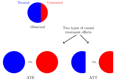
Figure 1: Illustration of the actual observed population, compared to the counterfactual target populations when estimating average treatment effects on the treated (ATT) and average treatment effects (ATE).

Our causal model for estimating the ATT is spelt out in Section 2, while Farewell’s linear increments model is formally introduced in Section 3. The relationship to mediation is demonstrated in Section 4. In Section 5 we discuss a shortcut through regression that yields an easier implementation of the method. We also briefly discuss estimation in Cox proportional hazards models. The application to the Swiss HIV Cohort data is found in Section 6, while results from simulations are summaried in Section 7. A discussion is given in Section 8. Details on the simulations and R code for carrying out the analyses, combined with a package for Farewell’s linear increments model (Hoff et al., 2014), is available in an online appendix.

2 A counterfactual additive hazards model for the treatment effect on the treated

2.1 The causal estimand of interest

The target estimand in this paper is the ATT for a time-to-event outcome in a setting with time-dependent exposure and confounding. Consider the illustration in Figure 2, depicting the situation for a hypothetical individual that starts treatment at some time point $S$. The time scale is time since inclusion in the study. When treatment is started, we can imagine a counterfactual scenario where treatment was not started at time $S$, and the individual remained untreated. Let $T^{S}$ be the potentially observed time of the outcome of interest when treatment is actually started at time $S$ and let $T^{S\ast}$ be the potential event time in the counterfactual situation that treatment is not started at time $S$ (or later).

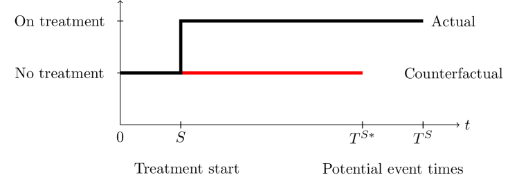
Figure 2: Illustration of the counterfactual scenarios in terms of event times, with $S$ being the time of treatment initiation, $T^{S}$ the event time under the given treatment and $T^{S*}$ the event time given no treatment. The black line denotes the observed outcome and the red line the unobserved counterfactual, given that treatment was never initiated.

In order to achieve notational clarity, we express the hazard rates in terms of conditional probabilities. Assume $S=s$ and let $h^{1}(t;s)$ be the causal hazard rate under the actual treatment initiation at $s$, for $t\geq s$. We can then write

$$h^{1}(t;s) =\frac{1}{dt}P(T^{S}\leq t+dt\,|\,S=s,T^{S}>t)$$

$$=E\left[\frac{1}{dt}P(T^{S}\leq t+dt\,|\,S=s,L^{1},T^{S}>t)\,|\,S=s,T^{S}>t\right],$$ (1)

where the second line in the formula follows from the Innovation theorem (Aalen et al., 2008). Note that $S=s$ represents conditioning, while $T^{s}$ is the result of a $do$-operator; that is the survival time under $do(\mathrm{treatment}$ starts at $s)$, where $S$ is a random variable. $L^{1}$ is the value of the corresponding covariate process under this same intervention.

Similarly, the causal hazard rate for the counterfactual scenario where treatment is not started at $s$ (or later), $h^{0}(t;s)$, can be written:

$$h^{0}(t;s) =\frac{1}{dt}P(T^{S\ast}\leq t+dt\,|\,S=s,T^{S\ast}>t)$$

$$=E\left[\frac{1}{dt}P(T^{S\ast}\leq t+dt\,|\,S=s,L^{0},T^{S\ast}>t)\,|\,S=s,T^{S\ast}>t\right],$$ (2)

where $T^{S\ast}$ is the potential survival time under the intervention $do(\mathrm{no}$ treatment$)$. Notice that we still condition with respect to treatment start at time $S=s$, but that counterfactually treatment is not started. The notation $L^{0}$ denotes the value of the covariate process in this case. The classic distinction in causal inference between conditioning and intervention is important here. We condition on treatment start at $S$, that is, we limit the outcomes to the part of the sample space with this starting time. However, we then intervene to insure that treatment is not really started.

The causal hazard difference is then given as follows for $t\geq s$:

$$d(t;s) =h^{1}(t;s)-h^{0}(t;s).$$ (3)

Defining the causal effect of interest, we integrate the causal hazard difference over $s$ to get a marginal effect. The effect will then only be a function of $t$, and can be estimated. The average causal hazard difference is thus:

$$d^{*}(t)=E(d(t,S)\,|\,t>S)=E^{S}(d(t,S)),$$ (4)

which corresponds to the ATT for all observed versions of treatment, started at any time point $S$. $E^{S}(.)$ denotes the conditional expectation given $t>S$, computed over the distribution of $S$.

Note that, conceptually, this means that when treatment is started for an individual, we want to create a "copy" of that individual who does not start treatment and observe her or him under both scenarios. When looking at the entire study population, this corresponds to a randomised study at treatment start where randomisation determines whether the intended treatment is actually started or not. Hence, our target parameter $d^{*}(t)$ is the average effect of the treatment that was actually started, compared to no treatment.

2.2 Assumptions

We assume an additive hazards regression model for the event of interest, taking the form

$$\alpha(t;B,\mathbf{L})=\delta(t)B(t)+\gamma_{0}(t)c+\gamma_{1}(t)L_{1}(t)+\ldots+\gamma_{k}(t)L_{k}(t),$$ (5)

with parameters $\delta(t)$ and $\gamma_{m}(t)$, for $m=0,\ldots,k$. Here, $c$ denotes a vector of baseline covariates, including a constant, and $\gamma_{0}(t)$ is a vector of time-dependent coefficients. The covariate processes $\mathbf{L}(t)=(L_{1}(t),\ldots,L_{k}(t))$ are various time-dependent quantities that may influence or be influenced by treatment. These processes are written as individual components and not in vector form since they are the main focus of interest; they are assumed to be measured repeatedly over time. The process $B(t)$ indicates whether treatment has been started; it is equal to zero with no treatment and changes to 1 when treatment starts. It is assumed that once started, treatment continues, so $B(t)$ cannot return to zero.

Assume that the model in Equation (5) is a causal model in the following sense: If one manipulates (intervenes on) the processes $\mathbf{L}(t)$ or $B(t)$, then the parameter functions $\delta(t)$ and $\gamma_{0}(t),\ldots,\gamma_{k}(t)$ in Equation (5) are assumed to stay unchanged. This implies that the assumption of no unmeasured confounding is met. For causal modelling in the setting of stochastic processes, see Røysland (2012).

Note that in our observed data, by definition, $B(S)=1$, but we also imagine a counterfactual scenario where $B(t)$ was manipulated to be 0 for $t\geq S$. In other words, we consider the situation where the person on treatment was not actually put on treatment and ask what would have happened then. The covariate processes of this non-treated scenario, where treatment is not started at time $S=s$ or later, are denoted $\mathbf{L}^{0}(t;s)=(L_{1}^{0}(t;s),\ldots,L_{k}^{0}(t;s))$; these are unobserved counterfactual quantities. We will therefore assume that we have a model for estimating these counterfactual individual covariate processes. The procedure we use for doing so, which is based on Farewell’s linear increments model for missing longitudinal data, and the corresponding causal assumptions are described in detail in Section 3. The covariate process under the scenario that treatment is actually started at time $S=s$ are denoted $\mathbf{L}^{1}(t;s)=(L_{1}^{1}(t;s),\ldots,L_{k}^{1}(t;s))$ and correspond to the actually observed processes $\mathbf{L}(t)$ for $t\geq s$.

2.3 Identification

The additive structure of the model in Equation (5) leads to the following formulation for the hazard rates in Equation (2) and (1):

$$h^{1}(t;s) =\delta(t)+\gamma_{0}(t)c+E\left[\gamma_{1}(t)L_{1}^{1}(t)+\ldots+\gamma_{k}(t)L_{k}^{1}(t)\,|\,S=s,T^{S}>t\right]$$ (6)

$$=\delta(t)+\gamma_{0}(t)c+\gamma_{1}(t)\tilde{L}_{1}^{1}(t;s)+\ldots+\gamma_{k}(t)\tilde{L}_{k}^{1}(t;s),$$

where $\tilde{L}_{i}^{1}(t;s)=E\left[L_{i}^{1}(t;s)\,|\,S=s,T^{S}>t\right]$, and

$$h^{0}(t;s) =\gamma_{0}(t)c+E\left[\gamma_{1}(t)L_{1}^{0}(t)+\ldots+\gamma_{k}(t)L_{k}^{0}(t)\,|\,S=s,T^{S\ast}>t\right]$$

$$=\gamma_{0}(t)c+\gamma_{1}(t)\tilde{L}_{1}^{0}(t;s)+\ldots+\gamma_{k}(t)\tilde{L}_{k}^{0}(t;s)$$

where $\tilde{L}_{i}^{0}(t;s)=E\left[L_{i}^{0}(t)\,|\,S=s,T^{S\ast}>t\right]$.

The corresponding causal hazard difference in Equation (3) can then be written as follows for $t\geq s$:

$$d(t;s) =\delta(t)+\gamma_{1}(t)(\tilde{L}_{1}^{1}(t;s)-\tilde{L}_{1}^{0}(t;s))+\ldots+\gamma_{k}(t)(\tilde{L}_{k}^{1}(t;s)-\tilde{L}_{k}^{0}(t;s)).$$ (7)

When defining the causal effect, we shall integrate the causal hazard difference over $s$ to get a marginal effect. The effect will then only be a function of $t$, and can be estimated. The average causal hazard difference is thus:

Using Equation (7) we can then identify the ATT in (4) using

$$d^{*}(t)= \delta(t)+\gamma_{1}(t)(E^{S}(\tilde{L}_{1}^{1}(t;S))-E^{S}(\tilde{L}_{1}^{0}(t;S)))$$

$$+\ldots+\gamma_{k}(t)(E^{S}(\tilde{L}_{k}^{1}(t;S))-E^{S}(\tilde{L}_{k}^{0}(t;S))).$$ (8)

2.4 Estimation

We will now discuss how to estimate the various components going into $d^{*}(t)$. Assume that a number of individuals, $i=1,\ldots,n$, participate in the study. Let $R(t)$ be the set of individuals for which $S_{i}<t$, and who are still under observation (i.e. the event has not happened and no censoring has occurred). Let $r(t)$ denote the size of $R(t)$ and assume that $r(t)>0$ from time 0. For simplicity, we assume independent censoring (see e.g. Aalen et al. (2008)), but in the case of dependent censoring, one can also adjust for this using inverse probability of censoring weighting.

First, the cumulative regression functions $\Delta(t)$ and $\Gamma_{1}(t),\ldots,\Gamma_{k}(t),$ defined as the integrals from 0 to $t$ of $\delta(t)$ and $\gamma_{1}(t),\ldots,\gamma_{k}(t)$, are estimated with an additive hazards model from all individuals, including those on and those off treatment, using the actual observed $\bm{L}$’s and treatment status. The estimates are denoted by $\hat{\Delta}(t)$ and $\hat{\Gamma}_{0}(t),\ldots,\hat{\Gamma}_{k}(t)$.

Then, we estimate $a_{j}(t)=E^{S}(\tilde{L}_{j}^{1}(t;S))$. When $t>S$, then all individuals are observed to be on treatment and hence an estimate is given as follows:

$$\hat{a}_{j}(t)=\frac{1}{r(t)}\sum_{i\in R(t)}L_{j}(t).$$

Note that we here make use of the consistency assumption, which means that “a subject’s counterfactual outcome under the same treatment regime that he actually followed is, precisely, his observed outcome” (Hernán et al., 2009).

Finally, we shall estimate

$$b_{j}(t)=E^{S}(\tilde{L}_{j}^{0}(t;S)).$$ (9)

This is a counterfactual quantity, and shall be estimated by Farewell’s linear increments model as described in Section 3. The resulting estimate is denoted by $\hat{b}_{j}(t)$. The estimated average cumulative causal effect based on Equation (8) is then given by

$$\hat{D^{*}}(t)=\hat{\Delta}(t)+\sum_{j=1}^{k}\int_{0}^{t}(\hat{a}_{j}(u)-\hat{b}_{j}(u))d\hat{\Gamma}_{k}(u).$$ (10)

Since we only consider treated individuals and compare with individuals that are identical apart from counterfactually not being on treatment, this is an estimate for a treatment effect of the treated.

3 Estimating counterfactual covariate processes when treatment is not started

So far we have shown how to estimate the causal effect of interest given that we can impute estimates of the confounder processes in the counterfactual setting that treatment had not been started. We shall view this as a missing data problem (Howe et al., 2015). We now give a general description of Farewell’s linear increments model and show how this model can be used to estimate the missing counterfactual quantities.

3.1 Farewell’s linear increments model

The linear increments model is a dynamic model for longitudinal data, analogous to the counting process approach for survival data. The model was originally suggested by Farewell (2006) and further described and discussed in Diggle et al. (2007). It was designed to analyse, in a simple manner, missing data in longitudinal studies. A multivariate generalisation of the model was given in Aalen and Gunnes (2010). Applications include estimation of mean response in studies with drop-out (Gunnes et al., 2009a) and correcting for missing data when assessing quality of life in a randomised clinical trial (Gunnes et al., 2009b). An R-package, FLIM, is available for fitting linear increments models (Hoff et al., 2014).

Let us start by imagining the complete data set (i.e. without missing data): Let $\widetilde{K}(t)$ be an $n\times m$ matrix of multivariate individual responses defined for a set of times $t\in\{0,\ldots,j\}$, with $\widetilde{K}(0)=k_{0}$, where the matrix $k_{0}$ contains the fixed starting values for the processes. The number of columns in $\widetilde{K}(t)$ corresponds to the number of $m$ variables measured for an individual and the number of rows corresponds to the number of $n$ individuals.

We define the increment $\Delta\widetilde{K}(t)=\widetilde{K}(t)-\widetilde{K}(t-1)$ and assume, for each $t$, that $\Delta\widetilde{K}(t)$ satisfies the model

$$\Delta\widetilde{K}(t)=\widetilde{K}(t-1)\beta(t)+\widetilde{\varepsilon}(t),$$ (11)

where $\beta(t)$ is a $m\times m$ parameter matrix and $\widetilde{\varepsilon}(t)$ is an $n\times m$ error matrix. The errors are defined as zero mean martingale increments such that $\mathrm{E}(\widetilde{\varepsilon}(t)\mid\mathcal{F}_{t-1})=0$, where $\mathcal{F}_{t}$ is the history of $K(t)$ up to and including time $t$. It then follows that

$$\mathrm{E}(\Delta\widetilde{K}(t)\mid\mathcal{F}_{t-1})=\widetilde{K}(t-1)\beta(t).$$

In analogy with censoring in survival analysis, missing data is common in longitudinal data. Let $\Delta K(t)$ denote the actually observed increments, i.e. when both components defining the increment are observed, and set $\Delta K(t)$ equal to zero otherwise. The relation between the true and observed responses and increments are $\Delta K(t)=Q(t)\Delta\widetilde{K}(t)$, where $Q(t)$ is a $n\times n$ diagonal matrix defined as follows: For individual $i$, the $i$’th diagonal element of $Q(t)$ is equal to 1 when the increment $\Delta\widetilde{K}_{i}(t)$ is observed and 0 otherwise. Let $\mathcal{Q}_{t}$ denote the history of the process $Q(t)$, that is, up to and including time $t$.

3.2 Causal assumptions of the linear increments model

The key condition for proper modelling of missing longitudinal data using the linear increments models is typically formulated trough the assumption of discrete-time independent censoring (DTIC), as discussed in Diggle et al. (2007). This assumption, which is analogous to the independent censoring assumption of survival analysis (see e.g. Aalen et al. (2008)), places constraints on the expected values of the increments $\Delta\widetilde{K}(t)=\widetilde{K}(t)-\widetilde{K}(t-1)$ of the hypothetical response, and can be formulated as follows:

$$\mathrm{E}(\Delta\widetilde{K}(t)\mid\mathcal{F}_{t-1},\mathcal{Q}_{t})=\mathrm{E}(\Delta\widetilde{K}(t)\mid\mathcal{F}_{t-1}),\quad\mathrm{for}\text{ }\mathrm{all}\text{ }t.$$

The DTIC assumption has a close relationship to other no-confounders assumptions, like sequentially missing at random (Seaman et al., 2016). In order to follow the assumptions as formulated in counterfactual analyses from causal inference, we will assume the slightly stronger condition of sequential conditional exchangeability. This assumption can for the modelling of missing longitudinal data be formulated as

$$\Delta\widetilde{K}(t)\perp Q(t)\mid\mathcal{F}_{t-1},\mathcal{Q}_{t-1},\quad\mathrm{for}\text{ }\mathrm{all}\text{ }t$$

e.g. based on the definition in Hernán et al. (2009).

Sequential conditional exchangeability guarantees that the observed data will satisfy the model defined in (11), so that we can write

$$\Delta K(t)=Q(t)K(t-1)\beta(t)+\varepsilon(t).$$

3.3 Estimation of missing covariate values

The procedure for estimating missing covariate values is as follows: We assume a nonparametric model over time, so that there is no assumed connection between $\beta(t_{1})$ and $\beta(t_{2})$ for two different times $t_{1}$ and $t_{2}$. The parameter matrices $\beta(t)$ can then be estimated unbiasedly by the least squares approach from observed increments, where we denote these estimates as $\hat{\beta}(t)$. The least square estimate of $\beta(t)$ is given by

$$\hat{\beta}(t)=(U^{T}U)^{-1}U^{T}\Delta K(t),$$

where $U=Q(t)K(t-1)$.

Now, let $Q_{0}(t)$ be an indicator which is equal to 1 when the value $\widetilde{K}(t)$ is observed. The hypothetical complete predicted data values can be estimated iteratively by (Aalen and Gunnes, 2010)

$$\widetilde{K}^{\mathrm{est}}(0) =k_{0},$$

$$\Delta\widetilde{K}^{\mathrm{est}}(t) =(1-Q_{0}(t))\widetilde{K}^{\mathrm{est}}(t-1)\hat{\beta}(t)+Q_{0}(t)(K(t)-\widetilde{K}^{\mathrm{est}}(t-1)),\quad t=1,\ldots,j$$ (12)

$$\widetilde{K}^{\mathrm{est}}(t) =\widetilde{K}^{\mathrm{est}}(t-1)+\Delta\widetilde{K}^{\mathrm{est}}(t),\qquad t=1,\ldots,j$$

given some initial values $k_{o}$. Note that when observation takes place, the estimated value $\widetilde{K}^{\mathrm{est}}(t)$ simply equals $K(t)$. When there is no observation, the increments are updated according to the model.

Farewell’s linear increments model will now be used below for estimating missing counterfactual values of covariate processes. For more details on the properties of this model, see Diggle et al. (2007) and Aalen and Gunnes (2010).

3.4 Application to imputing counterfactual trajectories

The counterfactual values $b_{j}(t)$ from Equation (9) shall be estimated by Farewell’s linear increments model. Assuming sequential conditional exchangeability, this model can give us a precise prescription for how to model missing data, which is central when estimating causal effects. Being exchangeable now means that the risk of event among the untreated would have been the same as the risk of event among the treated had subjects in the untreated group received the treatment (and vice versa). In a longitudinal setting this means that "at every observation time $k$ and conditional on prior treatment and covariate history, the treated and the untreated are exchangeable" (Hernán et al., 2009). This is also known as a no unmeasured confounding assumption.

We shall apply the linear increments model to the process $\mathbf{L}$. We then regard the values prior to treatment start as observed. When treatment is started the observations that would have been made in the absence of treatment are missing. These are estimated by the iterative procedure in Equation (12). If treatment is started at time $s$ we thus estimate the quantity $\tilde{L}_{j}^{0}(t;s)$ for each $j$. Taking an average of these at time $t$ over all individuals in $R(t)$ gives an estimate of $b_{j}(t)$. Notice from the definition of $R(t)$ in Section 2.4 that estimation of counterfactual trajectories will only take place until the individual is censored or experiences an event in the observed data. An illustration of the imputation idea is given in Figure 3.

An example showing how to impute counterfactual covariate values using the linear increments models has recently been included in the R package FLIM (Hoff et al., 2014).

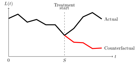
Figure 3: Illustrating the imputation of counterfactual covariate trajectories by Farewell’s linear increments model. Black line illustrates observed covariate trajectory and red line the originally unobserved, imputed counterfactual covariate trajectory for a hypothetical individual.

4 A mediation point of view

Mediation can also be studied for causal effects defined in an ATT setting, see e.g. Vansteelandt and VanderWeele (2012). We shall show that the formula for $d^{*}(t)$ in Equation (8), can be interpreted as the sum of a direct effect on the treated $\delta(t)$ and of an indirect effect transmitted through the covariates. This can be made precise as follows:

The natural direct effect is the effect that would be observed if the mediator under treatment was manipulated to be equal to the natural value of the mediator under no treatment. However, in our survival setting it is possible that the individual might survive in one counterfactual world and not in the other one, therefore manipulation at the individual level may not make sense. Instead we can use the concept of randomized interventional analogues of natural direct and indirect effects from VanderWeele (2015), see also standardized direct effects in Didelez et al. (2006).

Consider individuals that have started treatment. According to VanderWeele (2015, Section 5.4.1); “we will consider what would have happened if we fixed their mediator to a level that is drawn randomly from the subpopulation that is unexposed. Thus instead of using the individual’s particular value for the mediator in the absence of exposure, we use the distribution of the mediator amongst all the unexposed”. Our procedure follows the same idea in a slightly more general way, namely using the distribution of the mediator values among those not on treatment to estimate values of the mediator for those on treatment, where they not treated. This is precisely the calculation that is done by Farewell’s linear increments model.

For the purpose of estimating average effects we can formulate this for expected values. Assume that the mediator is the set of all time-dependent covariates; hence, we assume that $L_{i}^{1}(t;s)$ is manipulated to be equal to $L_{i}^{0}(t;s)$ for all $i$. The covariate part in Equation (8) would then be equal to 0, and so we would have

$$d^{*}(t)_{dir}=\delta(t)$$ (13)

as the average direct effect defined in the above sense. The average indirect effect is defined as the difference between the total causal effect and the direct effect; that is

$$d^{*}(t)_{indir} =\gamma_{1}(t)(E^{S}(\tilde{L}_{1}^{1}(t;S))-E^{S}(\tilde{L}_{1}^{0}(t;S)))$$

$$+\ldots+\gamma_{k}(t)(E^{S}(\tilde{L}_{k}^{1}(t;S))-E^{S}(\tilde{L}_{k}^{0}(t;S))).$$ (14)

A diagram illustrating a mediation model for $k=1$ is shown in Figure 4. The figure indicates that the causal effect may be seen as a sum of a direct effect, and an indirect effect passing through the covariate; the latter being the product of the coefficients on the two arrows.

Figure 4: Illustration of the mediation model for the causal effect of treatment on a time to event outcome from Equation (13) and (14) in the simple case of $k=1$.

Note that we have here a well defined composition valid at any time $t$. Based on this we can estimate cumulative direct and indirect effects from Equation (10), that is:

$$\hat{D^{*}}(t)_{dir}=\hat{\Delta}(t),\qquad\hat{D^{*}}(t)_{indir}=\sum_{j=1}^{k}\int_{0}^{t}(\hat{a}_{j}(u)-\hat{b}_{j}(u))d\hat{\Gamma}_{k}(u).$$ (15)

5 A shortcut through regression

A simple regression analysis can give us an approximate estimate of the causal effect in Equation (10). To do such an analysis one only needs to manipulate the values of the time-varying covariates in the original dataset, by giving individuals on treatment the imputed covariate values which they would have had, if they were, counterfactually, untreated. The manipulated dataset can then be analysed in a standard regression, adjusting for treatment, baseline covariates and the partly manipulated time-varying covariates. The regression function for the treatment covariate would then be the approximate estimate of the causal treatment effect.

Why should this work? The idea is that if those on treatment are given counterfactual covariates corresponding to no treatment, then the difference in outcome between treated and untreated must be due to the treatment. The same idea has worked well in the two-stage approach of Kennedy et al. (2010) and Taylor et al. (2014). The setting of these papers are different but the basic concept is the same.

5.1 The additive hazards model

The validity of the shortcut is best shown for additive models. We shall show later, in simulations, that the results are very close to those found by the direct approach in Section 2. However, we do not get exact theoretical results as we did in Section 2.

To put it formally: For an individual starting on treatment at time $s$, the hazard rate of an event from Equation (6) can be rewritten as follows $\mathrm{for\;}t\geq s$:

$$h^{1}(t;s) =\delta(t)+\gamma_{0}(t)c+\gamma_{1}(t)\tilde{L}_{1}^{1}(t;s)+\ldots+\gamma_{k}(t)\tilde{L}_{k}^{1}(t;s)$$

$$=d(t;s)+\gamma_{0}(t)c+\gamma_{1}(t)\tilde{L}_{1}^{0}(t;s)+\ldots+\gamma_{k}(t)\tilde{L}_{k}^{0}(t;s)$$

For individuals not on treatment, that is, $t<s$, the hazard rate is given by

$$h(t;0,\mathbf{L})=\gamma_{0}(t)c+\gamma_{1}(t)L_{1}(t)+\ldots+\gamma_{k}(t)L_{k}(t).$$

This is consistent with the following additive hazards regression model applied to all individuals at risk:

$$\mu(t)=\gamma_{0}(t)c+d(t,s)B(t)+\gamma_{1}(t)L_{1}^{\ast}(t,s)+\ldots+\gamma_{k}(t)L_{k}^{\ast}(t,s),$$

where $B(t)$ is the treatment indicator as defined earlier, and $L_{i}^{\ast}(t)$ equals $\tilde{L}_{j}^{0}(t;s)$ if $B(t)=1$ and $L_{i}(t)$ if $B(t)=0$. Note that for those on treatment we put in counterfactual values of the covariates to mimic what they would have were they not on treatment; this is the crux of the procedure. The causal effect for an individual starting treatment at time $s$ is seen to equal the coefficient of the variable $B(t)$. Note that this coefficient is dependent on the value of $S$, and is hence random (i.e. varying between individuals). If we knew the values of $\tilde{L}_{j}^{0}(t;s)$ and could run this regression we would expect that the coefficient corresponding to the covariate $B(t)$ would be an average of the possible values, and thus a reasonable estimate of $d^{*}(t)$. Since we estimate the cumulative coefficient in the additive regression model, we actually estimate $D^{*}(t)$, denoting this estimate $\tilde{D^{*}}(t)$. This is an approximate procedure since the coefficient of $B(t)$ varies with the individual treatment starting time $S$, thus we have a varying coefficient regression model. However, simulations show that $\tilde{D^{*}}(t)$ is very close to $\hat{D^{*}}(t)$ as might be expected. In fact, the simulations in Section 7 indicate that the two approaches estimate almost exactly the same thing.

The procedure depends on estimating the $\tilde{L}_{j}^{0}(t;s)$, which shall be done as previously, using Farewell’s linear increments model. Since we have a precise argument for $\hat{D^{*}}(t)$ and a less precise one for $\tilde{D^{*}}(t)$, the first one might be seen as more reliable. However, $\tilde{D^{*}}(t)$ is slightly easier to compute and fits with ideas already in the literature (Kennedy et al., 2010; Taylor et al., 2014).

5.2 The Cox model

Since the Cox model is the most common one in survival analysis, it is natural to ask whether the present approach could be applied to this model as well. The formal mathematical arguments in Section 2 and the causal effect given in Equation (10) does not work in this case; however, the intuitive argument given in Section 5 makes sense for the Cox model as well. Hence, one would expect that the shortcut method might work for the Cox model. The hazard rate would then be:

$$\mu(t)=\exp(\gamma_{0}(t)c+d(t,s)B(t)+\gamma_{1}L_{1}^{\ast}(t,s)+\ldots+\gamma_{k}L_{k}^{\ast}(t,s))$$

Again, we have a random coefficient model. What will be estimated by a Cox model is some kind of average of the quantity $d(t,s)$. Preliminary simulation in Section 7.4 seems to indicate that this might give sensible results, but further work on this issue is required.

6 Application to data from the Swiss HIV Cohort Study

Let us now consider data from The Swiss HIV Cohort Study (2010), studying the effect of antiretroviral treatment (HAART) on time to AIDS or death. The dataset we analyse consists of 2161 HIV infected individuals, with baseline at the time of the first follow-up after January 1996. The data is organised in monthly intervals, with time-varying variables describing the treatment received, CD4 cell count, viral load (HIV-1 RNA), haemoglobin levels and other relevant clinical variables. Scheduled clinical follow-up with protocol defined laboratory tests takes place every sixth month and on average one additional intermediate routine laboratory test is also recorded. In months with no new observations, the last observation is carried forward. Baseline variables include sex, year at birth, registration date and transmission category. The same dataset has been analysed before in Sterne et al. (2005); Gran et al. (2010); Røysland et al. (2011).

When estimating the effect of antiretroviral treatment on time to AIDS or death, time-dependent prognostic factors such as CD4, viral load and haemoglobin levels are typically time-dependent confounders. Time-dependent confounding can be adjusted for using marginal structural models (see Sterne et al. (2005)) or the sequential Cox approach (see Gran et al. (2010)). We shall here apply our new method for analysing the ATT.

Let us consider the three time-dependent variables CD4 count, viral load and haemoglobin level. For all individuals in the dataset that started treatment, we estimate their counterfactual covariate trajectories had they stayed untreated, using the iterative procedure described in Section 3. The counterfactual covariate values are estimated from the time treatment started and until the individuals are censored or experience an event in the observed data. When estimating counterfactual covariates, we adjust for baseline variables sex, age at baseline, year at baseline and transmission category, together with the three time-dependent variables. The observed and estimated covariate trajectories for all untreated individuals are shown in Figure 5.

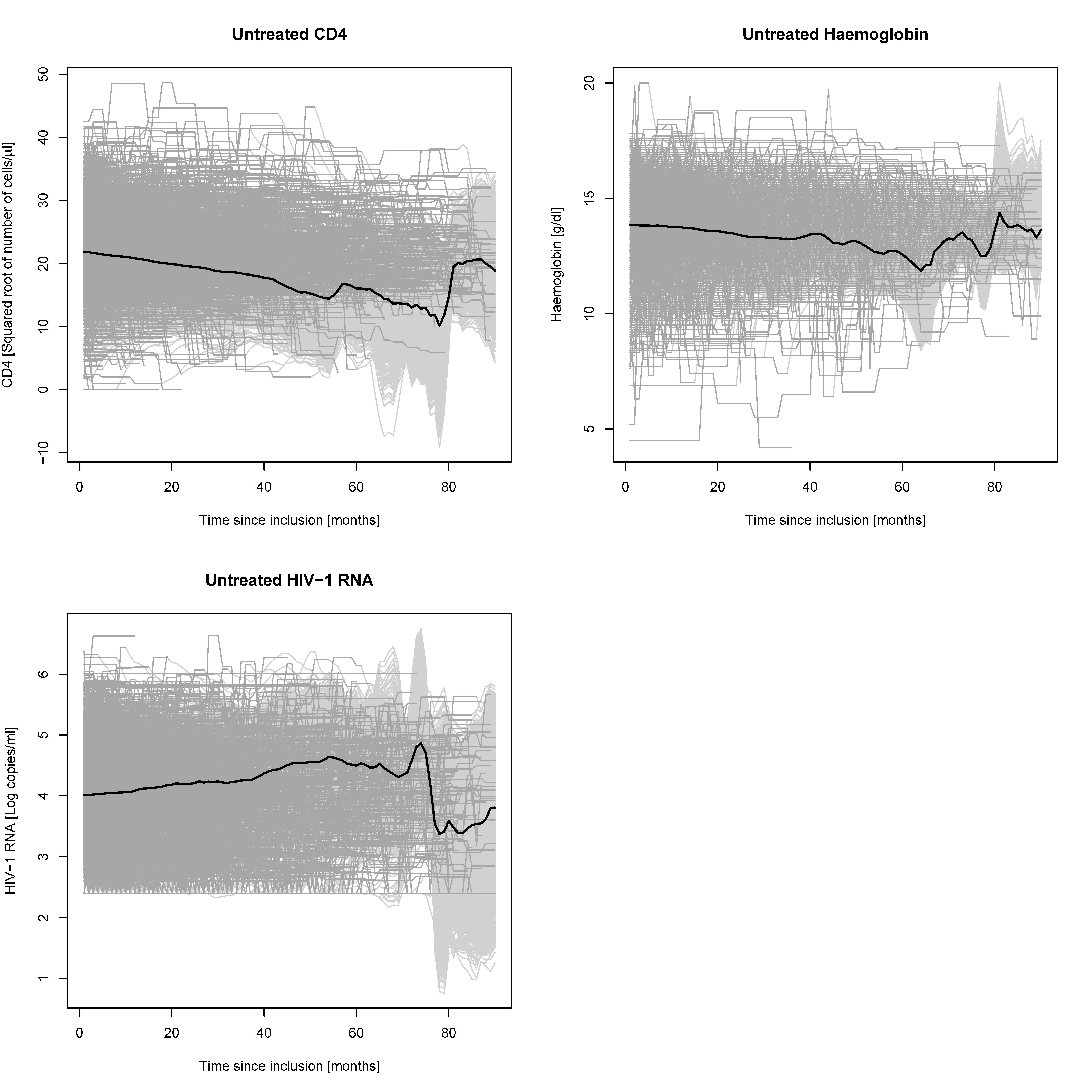
Figure 5: Observed (dark grey), estimated (light grey) and mean (black) CD4, viral load (HIV-1 RNA) and haemoglobin trajectories for untreated individuals.

Figure 5 shows that over time untreated individuals experience a decrease in CD4 and haemoglobin levels, and an increase in viral load. We see that the estimated (light grey) covariate trajectories typically depict individuals who are worse off, because they are modelled counterfactual trajectories, that is; trajectories for individuals who have started treatment in the observed data. This is best seen in the CD4 cell count trajectories because CD4 cell count is the most important predictor of treatment initiation. Note that model uncertainty gets bigger with time, as the size of the risk set decreases. This is seen by the increasing fluctuations of estimated CD4 counts with time. Because of this uncertainty the plots are truncated at 80 months, even though the last observation was 92 months after the start of follow-up.

The effect of treatment on the time-dependent covariates themselves can be studied graphically, by changing the time-scale to time since start of treatment and plotting the two counterfactual regimes of treated and untreated together (Figure 6). Here, the untreated group (the red lines) represent the unobserved counterfactual covariate trajectories the treated individuals would have had if they were not treated, which are all imputed values. For the treated group (black and grey lines), imputations are only needed when patients are censored. The rest of their trajectories are observed under treatment, as no individual, by definition, goes from being treated to untreated.

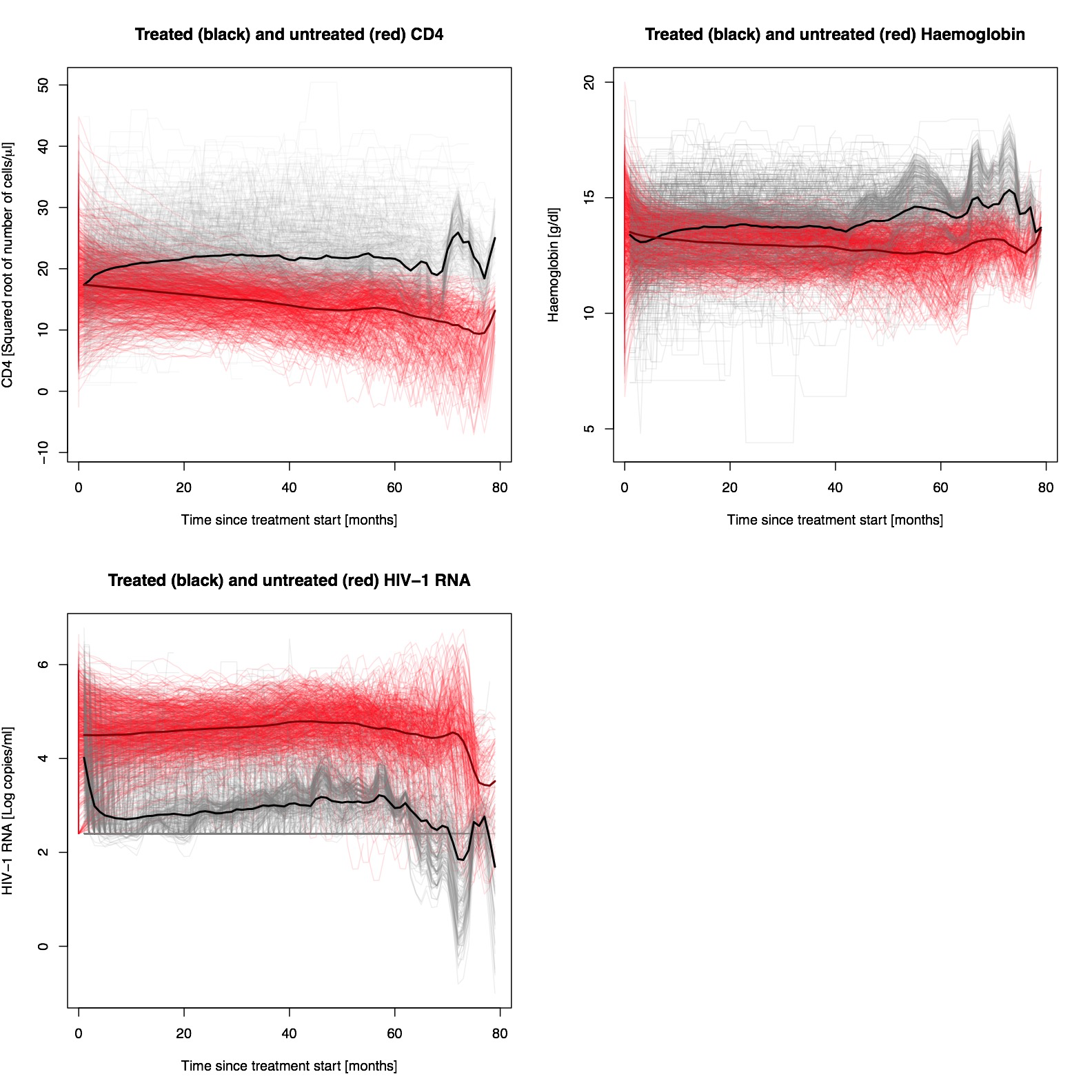
Figure 6: Observed, estimated and mean CD4, viral load (HIV-1 RNA) and haemoglobin trajectories for the two counterfactual regimes of treatment (black) and no treatment (red).

In Figure 6 we clearly see the negative consequences for untreated patients; lower CD4 counts and haemoglobin levels and higher viral load. Treated individuals, on the other hand, experience a rise in CD4 cell counts and a rather rapid decline in viral load.

Let us now return to the main objective of adjusting for time-dependent confounding. We want to estimate the treatment effect on the treated for antiretroviral treatment on time to AIDS or death, using the method in Section 2. In practice, we impute values for all counterfactual time-varying covariates under the scenario of no treatment, wherever these variables were not observed. The only time-varying variable we do not alter is the treatment indicator, representing the exposure we want to estimate, that is; the effect of treatment on time to AIDS or death.

We use the shortcut approach in Section 5 since it was demonstrated in Section 7 that it gives almost exactly the same result as the causal effect formula (10). The analysis was carried out fitting an additive hazards model to a pseudo dataset where all time-varying covariates for individuals on treatment were imputed using the linear increments model, adjusting for possible non-random dropout using inverse probability of censoring weights. The included covariates were HAART, sex, transmission category, baseline CD4 (sqrt cells per $\mu$L), baseline RNA (log10 copies per mL), baseline haemoglobin (g per mL), baseline CDC B event, previously experienced CDC B event at baseline, and current CD4, RNA and haemoglobin. The data is grouped into monthly intervals and baseline is set to the time of the first follow up visit after January 1996. For the marginal structural additive hazards model, the same covariates were used, except that the time-varying covariates were replaced by stabilised inverse probability of treatment weights. The applied censoring and treatment weights are identical to the weights used in Sterne et al. (2005), which analysed the same dataset.

Figure 7 (left panel) shows the cumulative treatment effect on the treated for HAART versus no treatment, found using the approach in Section 5.1. Treatment has a constant protective effect (a negative contribution to the hazard) for the first 30 months, before the effect decreases. The plot is truncated at 50 months to give a more detailed picture of the initial phase. As a comparison, in the second panel of Figure 7, we include the cumulative coefficient for HAART in a inverse probability weighted marginal structural Aalen additive model. This is merely a weighted additive hazards model using the same inverse probability of treatment and censoring weights as used in the marginal structural Cox proportional hazards model in Sterne et al. (2005). We see from Figure 7 that the estimated cumulative effects of treatment are somewhat smaller when using the marginal structural model. This is reasonable, since one would expect those actually treated to have a greater potential treatment effect on the average than those not actually treated.

Tests of effect (i.e. testing for slope) may be carried out for the plots in Figure 7, giving $p=0.0003$ for the left panel and $p=0.002$ for the right panel.

Figure 7: Analysis of the effect of HAART on AIDS or death in the Swiss HIV Cohort Study comparing estimates of the treatment effect on the treated (left panel) with average treatment effects (right panel). Both analyses are based on additive hazards regression, the first imputing counterfactual covariate trajectories from a linear increments model and secondly using an inverse probability weighted marginal structural model.

Note that robust confidence intervals are used for the curves in Figure 7. The intervals in the left panel may be slightly too narrow, as the uncertainty in the imputed values are not brought into the calculations of these intervals. An alternative is to calculate confidence intervals by bootstrapping.

All analyses were done in R version 3.0.0, using the aareg function from the package survival.

7 Simulation study

Let us now analyse simulated data to compare the methods and study their behaviour. The methods we want to compare are the procedures based on imputation of counterfactual covariate trajectories for estimating ATT, inverse probability weighted marginal structural models for estimating ATE and naive methods that do not properly adjust for time-dependent confounding.

To generate data with time-dependent confounding we simulate event times from an additive hazards model. We pretend to have a cohort of individuals under risk of experiencing some event of interest. Individuals are routinely controlled to have a covariate value measured. The probability of starting treatment on a specific time point will depend on an individual’s current covariate value, and in return, starting treatment affects the future covariate process. Both treatment status and the covariate value affect the probability of having an event.

7.1 Data generation

Imagine a cohort of $n$ individuals under risk of having an event $E(t)$, which can be postponed or prevented by treatment; everyone in the cohort starts out untreated. Each individual has a time-varying covariate $L(t)$ repeatedly measured on a set of pre-specified time points $t=0,1,...,11$, given that they have not yet experienced the event. To generate initial values of $L(t)$ for each subject, we took the square root of $n$ numbers uniformly distributed on the interval $[25,1000]$. The range of the interval and the square root transformation were employed to obtain a variable somewhat comparable to CD4 cell count. Untreated, $L(t)$ will decrease steadily, while when receiving treatment, $L(t)$ increase over time. Individuals who start treatment are not allowed to go back to being untreated. The hazard of having an event within an interval $[t,t+1)$ is affected by treatment status $B(t)$ and by covariate value $L(t)$. Everyone enter the study at $t=0$, and those who have not experienced the event by $t=11$ are censored.

We will consider three different treatment regimes, which are summarised in Figure 1 in the online appendix accompanying this paper. In the first, people with low covariate values have a high probability of starting treatment. The second regime is close to randomised treatment, meaning there are only small differences between treated and untreated individuals in terms of covariate values. Finally, the last regime is the opposite of the first, i.e, individuals with higher covariate values are prioritised for treatment. The online appendix also contains a pseudo code algorithm for simulating data under these three treatment regimes and the full corresponding R code. We ran the simulations 250 times, and in each run we generated a new dataset that was analysed with the methods described in the following section.

7.2 Analysing simulated data

The simulated data is analysed with the procedures for estimating the ATT as described in Section 2.4 and Section 5. For comparison, we also estimate the ATE from a marginal structural additive hazards model and treatment effects from two naive approaches. Implementing the marginal structural model involves estimating weights based on the inverse probabilities of starting treatment, which are then used in a weighted regression. The marginal structural model does correct for time-dependent confounding, but unlike our methods, the estimated effect of treatment is equivalent to comparing the effect of everyone being treated to no one being treated, as illustrated in Figure 1. The naive methods are additive regression analyses that do not properly correct for time-dependent confounding. In the first naive method we control for both treatment and covariate, and in the second we only control for treatment.

All of the methods are different implementations of Aalen’s additive hazards regression models, and we are interested in estimating the effect of treatment on survival. The estimated effects are displayed as curves showing the differences in cumulative hazards between the treated and untreated.

For the simulations, there are no single target parameter we can compare against to assess performance and check that methods are valid. Instead, we include an analysis of a simulated full counterfactual dataset. This dataset is constructed by combining data coming from the algorithm shown above where treatment is offered, with data from the same algorithm, but without offering treatment. This means that we end up with a dataset where those who originally received treatment are also included with their untreated histories. Analysing such a dataset with a univariable regression, controlling only for treatment, yields an estimate of the average treatment effect on the treated (ATT). In the simulation results, we will call this treatment effect on the treated: simulated.

Finally, we analyse the effect of treatment when starting treatment is randomised. This corresponds to finding the average treatment effect (ATE). More specifically, we implement a univariate regression, controlling only for treatment, to a dataset generated the same way as earlier, but with a flat probability set to 0.07 for starting treatment on all time points, for all individuals regardless of covariate values. The value 0.07 was chosen so that the random treatment setting was reasonably comparable to the other treatment regimes in terms of proportions of the cohort starting treatment at some point during follow-up.

7.3 Simulation results for the additive model

Figure 8 shows the mean of the cumulative hazard differences for being on treatment compared to not being on treatment. Both our proposed methods for estimating ATT in Section 2.4 and Section 5, the red curve and the dotted green curve, show similar estimates as the simulated target curve (blue) across all treatment regimes.

Our methods estimate the treatment effect on the treated. This effect varies between different treatment regimes. The marginal structural additive hazards model on the other hand, gives more or less the same curve estimates across the different regimes – estimates that are similar to the estimated treatment effect in a randomised study, the black dotted curve. The naive method where we control for both treatment and covariate value is estimating the direct effect of treatment, which is constant across all three simulations (the purple curves). The second naive method, green full-drawn line, where we only control for treatment, behaves very different from the advanced methods. In all but the second regime it fails to estimate a valid parameter, as it does not properly correct for the time-dependent confounding that is strong in regime 1 and regime 3.

The simulations show how our proposed methods estimate treatment effects that are dependent on who actually get treated. Given that we can impute counterfactual covariate trajectories, the procedures succeed in estimating the target curve that comes from analysing the full counterfactual dataset.

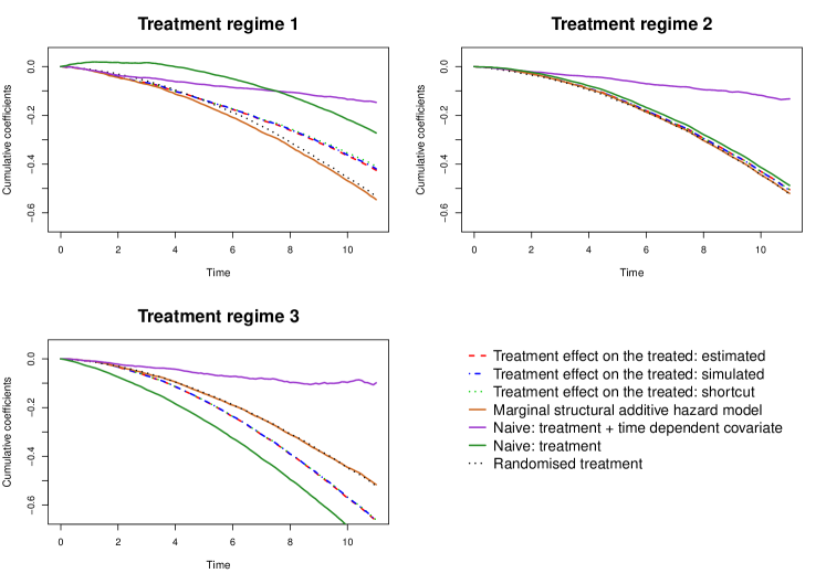
Figure 8: Average cumulative coefficients for the treatment effect for the three treatment regimes in the simulation study.

7.4 Simulation results for the Cox model

Treatment regime:	1	2	3
Treatment effect on the treated: simulated	0.77	0.74	0.69
Treatment effect on the treated: shortcut	0.79	0.75	0.68
Marginal structural model	0.75	0.74	0.75
Naive: treatment + time dependent covariate	0.93	0.93	0.91
Naive: treatment	0.84	0.76	0.64
Randomised treatment	0.75	0.75	0.75

Table 1: Cox model average hazard ratios for the effect of treatment.

Simulating data from Cox proportional hazards models with time-dependent confounding can be a very challenging task (Havercroft and Didelez, 2012), so instead we use the data already simulated for the additive model where, in contrary, simulation is very simple. This makes sense as it is quite clear that the Cox model, as well as other models, typically are used for data where the assumptions are not exactly fulfilled. In fact, one of the useful aspects of the Cox model is its robustness towards many types of model deviations.

The results from applying a Cox based analysis to the data simulated in Section 7 are presented in Table 1. We give all the same analyses as for the additive model apart from that based on Equation (10). Hence, the various settings are the same as previously and can be directly compared with the results for the additive model. First, one can see (in lines 1 and 2) that estimating the hazard ratio for the ATT using the shortcut approach gives essentially the same results as when simulating the same scenario. This indicates that the estimation method gives sensible results. In line 3 one sees that the marginal structural Cox model result in a hazard ratio that is independent of the treatment regime, as it should be, and that this fits with the randomised treatment (last line). The ATT analysis gives weaker effects than the ATE from the marginal structural model for regime 1, the same effect for regime 2, and stronger effects for regime 3. This again fits with the results for the additive model, and is as expected. The naive analyses also have the same type of deviations as seen for the additive model.

These are merely preliminary results, and obviously the issue of the validity of our approach for the Cox model needs further clarification.

8 Discussion

We have presented a new approach for estimating the ATT under time-dependent confounding. The ATT is a useful alternative to the ATE, and the two causal estimands answer two different questions. The latter answers the question how effective is the treatment if treatment was randomised over time?’, while the ATT answer the slightly different question of how effective was treatment for those who received it at the time they did? This is a subtle, but important difference, and it is not given that one should automatically use one method or the other when analysing data with time-dependent confounding – it depends on what questions one asks.

The ATT is a relevant parameter, both in a clinical and epidemiological setting, and quantifies the average effect of treatment as it was actually given. In other words; it quantifies the effect of the current treatment policy and not hypothetical ones. The ATT is often claimed to be a more relevant and preferred effect measure than the ATE in settings with selection among treated patients (Li et al., 2014). This is obviously the case in situations with time-dependent confounding, such as in the application to the Swiss HIV Cohort Study. The ATT for HIV treatment has been the target parameter in both early (Robins et al., 1992; Hernán et al., 2005) and recent papers (Wallace et al., 2016) using g-estimation. In settings were both the ATE and ATT can be identified, such as in our application, estimating both and comparing them will also add to the overall knowledge of the treatment effect. A difference between the two effect measures gives an indication on the effect of the current treatment policy.

Using the additive model gives an explicit derivation of the ATT in terms of counterfactual covariate processes. The positivity assumption is not as strict as when estimating the ATE, e.g. using inverse probability weighted marginal structural models, because there is no requirement that each individual should have a positive treatment probability. The no unmeasured confounding assumption is however still central. This also goes for the linear increments model when estimating counterfactual covariate processes, which we discussed earlier in terms of assuming conditional exchangeability. Another important assumption is the validity of the linear increments model itself. See VanderWeele (2013) for more on sensitivity analysis of unmeasured confounding in additive and proportional hazards models and Brumback et al. (2004) for more on sensitivity analysis with time-dependent confounding in HIV cohort studies.

Our approach for estimating the ATT also has the benefit of giving a detailed picture of how treatment works on the time-dependent variables themselves, and not only on the outcome. This of course comes at the cost of the assumptions for using the linear increments model, but in the application to data from the Swiss HIV Cohort Study we found that the this model provided stable and plausible estimates of counterfactual covariate trajectories. We have then shown that these estimates can be used to estimate the ATT in the presence of time-dependent confounding in survival data, by imputation in the additive hazards model. This can be seen as a front-door type of approach (Pearl, 2009), where causal effects are identified by estimating mechanisms, and our method may therefore also give additional insight into the dynamics of how treatment works.

Note that in our use of the linear increments model, the counterfactual covariate trajectories are only estimated until an individual experiences an event or is censored, as it can be seen in Figure 5. Covariate values beyond such events are not needed in order to fit our model for the overall treatment effect. However, for the sake of studying the effects of treatment initiation on the time-varying covariates themselves (and not on the main outcome) later covariate values might be useful. In that case, the linear increment model can be used to estimate covariate values after the time of censoring (or after the time of an event in the more conceptual case of immortal cohorts). See e.g. Diggle et al. (2007) for a further discussion of such topics.

Note also that the linear increments model is only one of many possible models that could be used for modelling of counterfactual covariate trajectories. Our approach could equally be used with other methods. Models that describe the progression of a specific disease using differential equations are another option, such as the HIV model in Prague et al. (2013). Different models, including a version of Farewell’s linear increments model, have also been compared in other papers (Prague et al., 2016).

Compared to other methods that estimate the ATT under time-dependent confounding on a time-to-event outcome our method is a two step approach, where each step has the benefit of being easy to implement using two simple existing statistical software packages. The outcome model also have the benefit of being a hazard regression model in the traditional sense, which typically is not the case in the g-estimation approach. We believe that there are advantages in considering several approaches for handling the thorny issue of time-dependent confounding, and that the procedure described in this paper serve as a valuable addition.

9 Acknowledgement

Jon Michael Gran, Rune Hoff and Odd O. Aalen were partly funded by the Research Council of Norway, project numbers 191460 and 218368. Kjetil Røysland was partly supported by the Norwegian Cancer Society contract/grant number 2197685.

References

- Aalen (1980) Aalen, O. (1980) A model for nonparametric regression analysis of counting processes. In Mathematical statistics and probability theory, 1–25. Springer.
- Aalen et al. (2014) Aalen, O., Røysland, K., Gran, J., Kouyos, R. and Lange, T. (2014) Can we believe the dags? a comment on the relationship between causal dags and mechanisms. Statistical methods in medical research, 0962280213520436.
- Aalen (1989) Aalen, O. O. (1989) A linear regression model for the analysis of life times. Statistics in medicine, 8, 907–925.
- Aalen et al. (2008) Aalen, O. O., Borgan, Ø. and Gjessing, H. K. (2008) Survival and event history analysis: a process point of view. Springer.
- Aalen and Gunnes (2010) Aalen, O. O. and Gunnes, N. (2010) A dynamic approach for reconstructing missing longitudinal data using the linear increments model. Biostatistics, 11, 453–472.
- Brumback et al. (2004) Brumback, B. A., Hernán, M. A., Haneuse, S. J. and Robins, J. M. (2004) Sensitivity analyses for unmeasured confounding assuming a marginal structural model for repeated measures. Statistics in medicine, 23, 749–767.
- Cole et al. (2013) Cole, S. R., Richardson, D. B., Chu, H. and Naimi, A. I. (2013) Analysis of occupational asbestos exposure and lung cancer mortality using the g formula. American journal of epidemiology, 177, 989–996.
- Daniel et al. (2013) Daniel, R., Cousens, S., De Stavola, B., Kenward, M. and Sterne, J. (2013) Methods for dealing with time-dependent confounding. Statistics in medicine, 32, 1584–1618.
- Didelez et al. (2006) Didelez, V., Dawid, P. and Geneletti, S. (2006) Direct and indirect effects of sequential treatments. In Proceedings of the Twenty-Second Conference Annual Conference on Uncertainty in Artificial Intelligence (UAI-06), 138–146. Arlington, Virginia: AUAI Press.
- Diggle et al. (2007) Diggle, P., Farewell, D. and Henderson, R. (2007) Analysis of longitudinal data with drop-out: objectives, assumptions and a proposal. Journal of the Royal Statistical Society: Series C (Applied Statistics), 56, 499–550.
- Edwards et al. (2014) Edwards, J. K., McGrath, L. J., Buckley, J. P., Schubauer-Berigan, M. K., Cole, S. R. and Richardson, D. B. (2014) Occupational radon exposure and lung cancer mortality: estimating intervention effects using the parametric g-formula. Epidemiology, 25, 829–834.
- Farewell (2006) Farewell, D. M. (2006) Linear models for censored data. Ph.D. thesis, University of Lancaster.
- Gran et al. (2010) Gran, J. M., Røysland, K., Wolbers, M., Didelez, V., Sterne, J. A., Ledergerber, B., Furrer, H., von Wyl, V. and Aalen, O. O. (2010) A sequential Cox approach for estimating the causal effect of treatment in the presence of time-dependent confounding applied to data from the Swiss HIV Cohort Study. Statistics in Medicine, 29, 2757–2768.
- Gunnes et al. (2009a) Gunnes, N., Farewell, D. M., Seierstad, T. G. and Aalen, O. O. (2009a) Analysis of censored discrete longitudinal data: estimation of mean response. Statistics in Medicine, 28, 605–624.
- Gunnes et al. (2009b) Gunnes, N., Seierstad, T. G., Aamdal, S., Brunsvig, P. F., Jacobsen, A.-B., Sundstrøm, S. and Aalen, O. O. (2009b) Assessing quality of life in a randomized clinical trial: Correcting for missing data. BMC medical research methodology, 9.
- Hansen (2008) Hansen, B. B. (2008) The prognostic analogue of the propensity score. Biometrika, 95, 481–488.
- Havercroft and Didelez (2012) Havercroft, W. and Didelez, V. (2012) Simulating from marginal structural models with time-dependent confounding. Statistics in medicine, 31, 4190–4206.
- Hernán et al. (2005) Hernán, M. A., Cole, S. R., Margolick, J., Cohen, M. and Robins, J. M. (2005) Structural accelerated failure time models for survival analysis in studies with time-varying treatments. Pharmacoepidemiology and drug safety, 14, 477–491.
- Hernán et al. (2009) Hernán, M. A., McAdams, M., McGrath, N., Lanoy, E. and Costagliola, D. (2009) Observation plans in longitudinal studies with time-varying treatments. Statistical Methods in Medical Research, 18, 27–52.
- Hoff et al. (2014) Hoff, R., Gran, J. M. and Farewell, D. (2014) Farewell’s linear increments model for missing data: The flim package. A peer-reviewed, open-access publication of the R Foundation for Statistical Computing, 137.
- Howe et al. (2015) Howe, C. J., Cain, L. E. and Hogan, J. W. (2015) Are all biases missing data problems? Current Epidemiology Reports, 1–10.
- Keil et al. (2014) Keil, A. P., Edwards, J. K., Richardson, D. R., Naimi, A. I. and Cole, S. R. (2014) The parametric g-formula for time-to-event data: towards intuition with a worked example. Epidemiology (Cambridge, Mass.), 25, 889.
- Kennedy et al. (2010) Kennedy, E. H., Taylor, J. M., Schaubel, D. E. and Williams, S. (2010) The effect of salvage therapy on survival in a longitudinal study with treatment by indication. Statistics in medicine, 29, 2569–2580.
- Li et al. (2014) Li, Y., Schaubel, D. E. and He, K. (2014) Matching methods for obtaining survival functions to estimate the effect of a time-dependent treatment. Statistics in biosciences, 6, 105–126.
- Martinussen and Vansteelandt (2013) Martinussen, T. and Vansteelandt, S. (2013) On collapsibility and confounding bias in cox and aalen regression models. Lifetime data analysis, 19, 279–296.
- Martinussen et al. (2011) Martinussen, T., Vansteelandt, S., Gerster, M. and Hjelmborg, J. v. B. (2011) Estimation of direct effects for survival data by using the aalen additive hazards model. Journal of the Royal Statistical Society: Series B (Statistical Methodology), 73, 773–788.
- Martinussen et al. (2016) Martinussen, T., Vansteelandt, S., Tchetgen, E. and Zucker, D. M. (2016) Instrumental variables estimation of exposure effects on a time-to-event response using structural cumulative survival models. arXiv preprint arXiv:1608.00818.
- Pearl (2009) Pearl, J. (2009) Causality: models, reasoning and inference. Cambridge Univ Press.
- Picciotto and Neophytou (2016) Picciotto, S. and Neophytou, A. M. (2016) G-estimation of structural nested models: Recent applications in two subfields of epidemiology. Current Epidemiology Reports, 3, 242–251.
- Pirracchio et al. (2013) Pirracchio, R., Carone, M., Rigon, M. R., Caruana, E., Mebazaa, A. and Chevret, S. (2013) Propensity score estimators for the average treatment effect and the average treatment effect on the treated may yield very different estimates. Statistical methods in medical research, 0962280213507034.
- Prague et al. (2016) Prague, M., Commenges, D., Gran, J., Ledergerber, B., Furrer, H., Thiébaut, R. et al. (2016) Dynamic versus marginal structural models for estimating the effect of haart on cd4 in observational studies: application to the aquitaine cohort study and the swiss hiv cohort study. Biometrics.
- Prague et al. (2013) Prague, M., Commenges, D. and Thiébaut, R. (2013) Dynamical models of biomarkers and clinical progression for personalized medicine: the hiv context. Advanced Drug Delivery Reviews, 65, 954–965.
- Robins et al. (1992) Robins, J. M., Blevins, D., Ritter, G. and Wulfsohn, M. (1992) G-estimation of the effect of prophylaxis therapy for pneumocystis carinii pneumonia on the survival of aids patients. Epidemiology, 319–336.
- Robins and Hernán (2009) Robins, J. M. and Hernán, M. A. (2009) Estimation of the causal effects of time-varying exposures. Longitudinal data analysis, 553–599.
- Robins et al. (2000) Robins, J. M., Hernan, M. A. and Brumback, B. (2000) Marginal structural models and causal inference in epidemiology. Epidemiology, 11, 550–560.
- Røysland (2012) Røysland, K. (2012) Counterfactual analyses with graphical models based on local independence. The Annals of Statistics, 40, 2162–2194.
- Røysland et al. (2011) Røysland, K., Gran, J. M., Ledergerber, B., von Wyl, V., Young, J. and Aalen, O. O. (2011) Analyzing direct and indirect effects of treatment using dynamic path analysis applied to data from the Swiss HIV Cohort Study. Statistics in Medicine, 30, 2947–2958.
- Seaman et al. (2016) Seaman, S. R., Farewell, D. and White, I. R. (2016) Linear increments with non-monotone missing data and measurement error. Scandinavian Journal of Statistics.
- Sterne et al. (2005) Sterne, J. A., Hernán, M. A., Ledergerber, B., Tilling, K., Weber, R., Sendi, P., Rickenbach, M., Robins, J. M. and Egger, M. (2005) Long-term effectiveness of potent antiretroviral therapy in preventing aids and death: a prospective cohort study. Lancet, 366, 378–384.
- Strohmaier et al. (2015) Strohmaier, S., Røysland, K., Hoff, R., Borgan, Ø., Pedersen, T. and Aalen, O. O. (2015) Dynamic path analysis-a useful tool to investigate mediation processes in clinical survival trials. arXiv preprint arXiv:1504.06506.
- Taubman et al. (2009) Taubman, S. L., Robins, J. M., Mittleman, M. A. and Hernán, M. A. (2009) Intervening on risk factors for coronary heart disease: an application of the parametric g-formula. International Journal of Epidemiology, 38, 1599–1611.
- Taylor et al. (2014) Taylor, J. M., Shen, J., Kennedy, E. H., Wang, L. and Schaubel, D. E. (2014) Comparison of methods for estimating the effect of salvage therapy in prostate cancer when treatment is given by indication. Statistics in medicine, 33, 257–274.
- Tchetgen Tchetgen et al. (2015) Tchetgen Tchetgen, E. J., Walter, S., Vansteelandt, S., Martinussen, T. and Glymour, M. (2015) Instrumental variable estimation in a survival context. Epidemiology, 26, 402–410.
- The Swiss HIV Cohort Study (2010) The Swiss HIV Cohort Study (2010) Cohort profile: the Swiss HIV Cohort Study. International journal of epidemiology, 39, 1179–1189.
- VanderWeele (2013) VanderWeele, T. J. (2013) Unmeasured confounding and hazard scales: sensitivity analysis for total, direct, and indirect effects. European journal of epidemiology, 28, 113.
- VanderWeele (2015) — (2015) Explanation in causal inference: methods for mediation and interaction. Oxford University Press.
- Vansteelandt et al. (2014a) Vansteelandt, S., Joffe, M. et al. (2014a) Structural nested models and g-estimation: The partially realized promise. Statistical Science, 29, 707–731.
- Vansteelandt et al. (2014b) Vansteelandt, S., Martinussen, T. and Tchetgen, E. T. (2014b) On adjustment for auxiliary covariates in additive hazard models for the analysis of randomized experiments. Biometrika, 101, 237–244.
- Vansteelandt and VanderWeele (2012) Vansteelandt, S. and VanderWeele, T. J. (2012) Natural direct and indirect effects on the exposed: effect decomposition under weaker assumptions. Biometrics, 68, 1019–1027.
- Wallace et al. (2016) Wallace, M. P., Moodie, E. E. and Stephens, D. A. (2016) Model assessment in dynamic treatment regimen estimation via double robustness. Biometrics.
- Westreich et al. (2012) Westreich, D., Cole, S. R., Young, J. G., Palella, F., Tien, P. C., Kingsley, L., Gange, S. J. and Hernán, M. A. (2012) The parametric g-formula to estimate the effect of highly active antiretroviral therapy on incident aids or death. Statistics in medicine, 31, 2000–2009.