Schrijver graphs
and projective quadrangulations

Abstract

In a recent paper [J. Combin. Theory Ser. B, 113 (2015), pp. 1–17], the authors have extended the concept of quadrangulation of a surface to higher dimension, and showed that every quadrangulation of the $n$-dimensional projective space $\mathbb{P}^{n}$ is at least $(n+2)$-chromatic, unless it is bipartite. They conjectured that for any integers $k\geq 1$ and $n\geq 2k+1$, the Schrijver graph $SG(n,k)$ contains a spanning subgraph which is a quadrangulation of $\mathbb{P}^{n-2k}$. The purpose of this paper is to prove the conjecture.

1 Introduction

Given any integers $k\geq 1$ and $n\geq 2k$, the Kneser graph $KG(n,k)$ is the graph whose vertex set consists of all $k$-subsets of $[n]=\left\{{1,\dots,n}\right\}$, and with edges joining pairs of disjoint subsets. It was conjectured by Kneser [5], and proved by Lovász [6] in 1978, that the chromatic number of $KG(n,k)$ is $n-2k+2$.

Schrijver [8] found a vertex-critical subgraph $SG(n,k)$ of $KG(n,k)$ whose chromatic number is also $n-2k+2$. (Recall that a graph is vertex-critical if the deletion of any vertex decreases the chromatic number.)

In [4], a quadrangulation of a space triangulated by a (generalised) simplicial complex $\mathsf{K}$ is defined as a spanning subgraph $G$ of the $1$-skeleton $\mathsf{K}^{(1)}$ such that the induced subgraph of $G$ on the vertex set of any maximal simplex of $\mathsf{K}$ is complete bipartite with at least one edge.

Particular attention was given in [4] to quadrangulations of projective spaces, and it was shown that if $G$ is a quadrangulation of the projective space $\mathbb{P}^{n}$, then the chromatic number of $G$ is at least $n+2$. By constructing suitable projective quadrangulations of $\mathbb{P}^{n}$ homomorphic to Schrijver graphs, an alternative proof of Schrijver’s result was obtained.

The purpose of this paper is to prove Conjecture 7.1 from [4] by establishing the following result:

Theorem 1.

For any $k\geq 1$ and $n>2k$, the graph $SG(n,k)$ contains a spanning subgraph $QG(n,k)$ that embeds in $\mathbb{P}^{n-2k}$ as a quadrangulation. In particular, $\chi(QG(n,k))=n-2k+2$.

To prove Theorem 1, we need to construct a suitable triangulation of the sphere $S^{n-2k}$. We first review some topological preliminaries (Section 2) and explore combinatorial relations among the vertices of Schrijver graphs (Section 3).

In Section 4, the required properties of the sought triangulation of $S^{n-2k}$ are formulated in Theorem 8, which is then proved by giving an explicit recursive construction. Theorem 1 is derived at the end of Section 4.

In Section 5, two open problems are given to conclude the paper. In particular, we conjecture that the graph $QG(n,k)$ of Theorem 1 is edge-critical.

2 Topological preliminaries

In this section, we recall the necessary topological concepts. For a background on topological methods in combinatorics, we refer the reader to Matoušek [7]. For an introduction to algebraic topology, consult Hatcher [2] or Munkres [3].

A simplicial complex $\mathsf{C}$ with vertex set $V$ is a hereditary set system on $V$; the elements of this set system are the faces of $\mathsf{C}$. A geometric simplicial complex $\mathsf{K}$ in $\mathbb{R}^{d}$ is obtained if we associate each vertex in $V$ with a point in $\mathbb{R}^{d}$ in such a way that

1. the set of points $P_{\sigma}$ associated with each face $\sigma$ is in convex position, and

2. for distinct faces $\sigma$ and $\tau$, the relative interiors of the convex hulls of $P_{\sigma}$ and $P_{\tau}$ are disjoint.

The convex hulls of the sets $P_{\sigma}$, where $\sigma$ is a face of the underlying simplicial complex $\mathsf{C}$, will be referred to as the faces of $\mathsf{K}$. Since we will be dealing exclusively with geometric simplicial complexes in this paper, we will often drop the adjectives ‘geometric’ and ‘simplicial’.

A face such as $\left\{{a,b,c}\right\}$ is also written as $abc$. Two vertices $v,w$ of $\mathsf{K}$ are adjacent if $vw$ is a face of $\mathsf{K}$. The dimension of a face $\sigma$ is $\left|{\sigma}\right|-1$. Faces of dimension one are called edges. The vertex set of a geometric simplicial complex $\mathsf{K}$ will be referred to as $V(\mathsf{K})$.

The space $\|\mathsf{K}\|$ of a geometric simplicial complex $\mathsf{K}$ in $\mathbb{R}^{d}$ is the subspace of $\mathbb{R}^{d}$ obtained as the union of all faces of $\mathsf{K}$. If a space $X\subseteq\mathbb{R}^{d}$ is homeomorphic to $\|\mathsf{K}\|$, we say that $\mathsf{K}$ triangulates $X$.

The induced subcomplex of $\mathsf{K}$ on a set $X\subseteq V(\mathsf{K})$, denoted by $\mathsf{K}[X]$, has vertex set $X$ and its faces are all the faces of $\mathsf{K}$ contained in $X$.

A $2$-coloured complex $\mathsf{K}$ in $\mathbb{R}^{d}$ is a geometric simplicial complex in $\mathbb{R}^{d}$, with each vertex coloured black or white. For any point $p\in\mathbb{R}^{d}$, its antipode is the point $-p$. The complex $\mathsf{K}$ is antisymmetric if the antipode $-v$ of every vertex $v$ is also a vertex of $\mathsf{K}$, and the colours of $v$ and $-v$ are different.

Suppose that $\mathsf{K}$ triangulates the ball $B^{d}$. The boundary of $\mathsf{K}$ is the subcomplex triangulating the boundary sphere $S^{d-1}=\partial B^{d}$. We will say that $\mathsf{K}$ is boundary-antisymmetric if its boundary is antisymmetric.

Let us recall the definition of deformation retraction (as given in [2]). Given a subspace $A$ of a topological space $X$, a family of continuous maps $f_{t}:\,X\to X$ (where $t\in[0,1]$) is a deformation retraction of $X$ onto $A$ if $f_{0}$ is the identity, so is the restriction of each $f_{t}$ to $A$, the image of $f_{1}$ is $A$, and the family is continuous when viewed as a map from $X\times[0,1]\to X$. If such a deformation retraction exists, $A$ is said to be a deformation retract of $X$.

Next, let $\mathsf{K}$ be a 2-coloured geometric complex whose space is a deformation retract of the thickened sphere $S^{d}\times I$ in $\mathbb{R}^{d+1}$, where $d\geq 1$, $S^{d}$ is the unit $d$-sphere and $I$ is a short interval in $\mathbb{R}$. Thus, we can define the interior of $\mathsf{K}$ as the bounded component of $\mathbb{R}^{d+1}\setminus\|\mathsf{K}\|$, and similarly for the exterior of $\mathsf{K}$. Note that the origin of $\mathbb{R}^{d+1}$ is contained in the interior. We define the interior boundary of $\mathsf{K}$, $\mathsf{IB}(\mathsf{K})$, as the subcomplex of $\mathsf{K}$ induced on the set of vertices contained in the closure of the interior of $\mathsf{K}$. The exterior boundary $\mathsf{EB}(\mathsf{K})$ is defined analogously. Note that $\mathsf{IB}(\mathsf{K})$ and $\mathsf{EB}(\mathsf{K})$ need not be disjoint.

In the above setting, we will utilise the operation of adding the clone of a vertex. For a vertex $v$ of $\mathsf{IB}(\mathsf{K})$, we add a vertex $v^{*}$ of the same colour (the clone of $v$) and embed it in the open segment from $v$ to the origin, very close to $v$. Furthermore, for each face $\sigma$ of $\mathsf{IB}(\mathsf{K})$ containing $v$, we add a face $\sigma\cup\left\{{v^{*}}\right\}$. Thus, $v^{*}$ replaces $v$ in the interior boundary of the resulting complex $\mathsf{K}^{\prime}$. Note also that $vv^{*}$ is a face of $\mathsf{K}^{\prime}$.

Let $K$ be a $2$-coloured complex and $u,v$ two adjacent vertices of $\mathsf{K}$ of the same colour. The contraction of the edge $uv$ is the operation replacing each face $\sigma$ of $\mathsf{K}$ with $\sigma\setminus\left\{{u,v}\right\}\cup\left\{{w}\right\}$, where $w$ is a new vertex (assigned the colour of $u$ and $v$). Geometrically, it corresponds to shrinking the segment $uv$ to a point. By definition, the operation does not introduce multiple copies of any face. For example, if $\mathsf{K}$ is the complex whose maximal faces are $xu$, $xv$ and $uvy$, where $u$ and $v$ are black and $x$ and $y$ are white, then the contraction of $uv$ produces the complex with maximal faces $xw$ and $wy$.

Let $\mathsf{K}$ and $\mathsf{L}$ be $2$-coloured complexes. A mapping $f:\,V(\mathsf{K})\to V(\mathsf{L})$ is a homomorphism (of $2$-coloured complexes) from $\mathsf{K}$ to $\mathsf{L}$ if $f$ preserves vertex colours and for any face $\sigma$ of $\mathsf{K}$, its image $f[\sigma]$ is a face of $\mathsf{L}$. (We stress that $f[\sigma]$ is a set, without repeated elements.)

A homomorphism $f$ from $\mathsf{K}$ to $\mathsf{L}$ is an isomorphism if $f$ is a bijection and $f^{-1}$ is a homomorphism.

For an antisymmetric $2$-coloured complex $\mathsf{K}$ triangulating a sphere, we define its associated graph $G(\mathsf{K})$ as the graph with vertex set $V(\mathsf{K})$ and with the edge set consisting of all edges of $\mathsf{K}$ with one end black and the other white.

3 Combinatorial preliminaries

Before we present the construction proving Theorem 1, we need to do some preparatory work. In this section, we introduce some terminology and notation that is useful for the classification of the vertices of the Schrijver graph $SG(n,k)$.

Let $k\geq 1$ and $n\geq 2k+1$. We let $C_{n}$ be the $n$-circuit on the vertex set $[n]=\left\{{1,\dots,n}\right\}$ and let $V(n,k)$ be the set of all independent subsets of $[n]$ of size $k$. Addition and subtraction on $[n]$ are defined ‘with wrap-around’: for instance, if $i,j\in[n]$ and $(i-1)+(j-1)\equiv\ell-1\pmod{n}$, where $\ell\in[n]$, then $i+j$ is defined as $\ell$. We let $V_{\,}(n,k)$ be the set of all subsets of $[n]$ of size $k$ that are independent sets in $C_{n}$. Note that $V_{\,}(n-1,k)$ is a subset of $V_{\,}(n,k)$.

The core of a set $A\in V_{\,}(n,k)$ is the set

$$\mathrm{core}(A)=\begin{cases}A\setminus\left\{{1}\right\}&\text{if $1\in A$,}\\ A\setminus\left\{{\max(A)}\right\}&\text{otherwise.}\end{cases}$$

Thus, $\mathrm{core}(\left\{{1,3,5}\right\})=\left\{{3,5}\right\}$, while $\mathrm{core}(\left\{{2,4,6}\right\})=\left\{{2,4}\right\}$.

Observation 2.

For $A\in V_{\,}(n,k)$,

$$\mathrm{core}(A)\cap\left\{{1,n}\right\}=\emptyset.$$

Let $0\leq i\leq n/2$. We define the set $\Lambda_{n,i}\subseteq[n]$ as follows:

$$\Lambda_{n,i}=\begin{cases}\left\{{2,4,\dots,i-1}\right\}\cup\left\{{n-i+1,n-i+3,\dots,n}\right\}&\text{if $i$ is odd,}\\ \left\{{1,3,\dots,i-1}\right\}\cup\left\{{n-i+1,n-i+3,\dots,n-1}\right\}&\text{if $i$ is even.}\end{cases}$$

For small $i$, the sets $\Lambda_{n,i}$ are given in the following table:

$\Lambda_{n,0}$	$\Lambda_{n,1}$	$\Lambda_{n,2}$	$\Lambda_{n,3}$	$\Lambda_{n,4}$
$\emptyset$	$\left\{{n}\right\}$	$\left\{{1,n-1}\right\}$	$\left\{{2,n-2,n}\right\}$	$\left\{{1,3,n-3,n-1}\right\}$

Note that for each $i$, $\Lambda_{n,i}\in V_{\,}(n,i)$.

The $n$-level of a set $A\in V_{\,}(n,k)$, $\ell^{n}(A)$, is the maximum $i$ such that $\Lambda_{n,i}\subseteq A$. Note that $0\leq\ell^{n}(A)\leq k$. For $0\leq i\leq k$, we define

$$V_{i}(n,k)=\left\{{A\in V_{\,}(n,k)}:\,{\ell^{n}(A)=i}\right\}.$$

Furthermore, we let $V_{+}(n,k)$ be the union of all $V_{i}(n,k)$ with $i\geq 1$.

Lemma 3.

We have

$$V_{0}(n,k)=V_{\,}(n-1,k).$$

Proof.

We need to show that for any set $A\in V_{\,}(n,k)$, we have $\ell^{n}(A)=0$ if and only if $A\in V_{\,}(n-1,k)$. By definition, $\ell^{n}(A)=0$ if and only if $A$ contains neither $\left\{{n}\right\}$ nor $\left\{{1,n-1}\right\}$ as a subset. In turn, this holds if and only if $A\in V_{\,}(n-1,k)$. ∎

Let $B\in V_{\,}(n-1,k)$. We define the set $B\langle n\rangle\in V_{\,}(n,k)$ by

$$B\langle n\rangle=\mathrm{core}(B)\cup\left\{{n}\right\}.$$

By Observation 2, the operation is well-defined. Since it will be used in relation with adding the ‘clone’ of a vertex labelled by $B$, we might call $B\langle n\rangle$ the $n$-clone of $B$.

The following lemma will be useful:

Lemma 4.

For $2k+1\leq i<m$ and $A\in V_{\,}(i-1,k)$, $(A\langle i\rangle)\langle m\rangle=A\langle m\rangle$.

Proof.

By definition, $A\langle i\rangle=\mathrm{core}(A)\cup\left\{{i}\right\}$. Since $1\notin\mathrm{core}(A)$, $\mathrm{core}(A\langle i\rangle)=\mathrm{core}(A)$. Thus, $(A\langle i\rangle)\langle m\rangle=A\langle m\rangle$. ∎

For a set $A\in V_{\,}(n,k)$ such that $1\notin A$, we define $A-1$ as the set obtained by subtracting $1$ from each element of $A$ (and similarly for $A+1$).

Let us define a mapping $f$ from $V_{\,}(n,k)$ to $V_{\,}(n-2,k-1)$, and a mapping $g_{n}$ in the inverse direction. Let $X\in V_{\,}(n,k)$ and $Y\in V_{\,}(n-2,k-1)$. The mappings are as follows:

$$f(X) =\mathrm{core}(X)-1,$$

$$g_{n}(Y) =\begin{cases}(Y+1)\cup\left\{{1}\right\}&\text{if $n-2\in Y$,}\\ (Y+1)\cup\left\{{n}\right\}&\text{otherwise.}\end{cases}$$

Lemma 5.

The restriction of $f$ to $V_{+}(n,k)$ is a bijection

$$f:\,V_{+}(n,k)\to V_{\,}(n-2,k-1),$$

and $g_{n}$ is its inverse. Furthermore, $f$ maps disjoint pairs of sets to disjoint pairs.

Proof.

The first assertion follows from the fact that the image of $g_{n}$ is contained in $V_{+}(n,k)$, and from the easily verified equalities

$$f(g_{n}(Y))=Y\text{\qquad and \qquad}g_{n}(f(X))=X$$

for $X\in V_{+}(n,k)$, $Y\in V_{\,}(n-2,k-1)$.

The assertion that the images of disjoint sets under $f$ are disjoint follows directly from the definition of $f$. ∎

Corollary 6.

All the sets in $V_{+}(n,k)$ have distinct cores.

Observation 7.

For any set $B\in V_{\,}(n-1,k)$, we have $f(B\langle n\rangle)=f(B)$. Thus, the suitable restriction of $f$ is a bijection

$$\left\{{B\langle n\rangle}:\,{B\in V_{+}(n-1,k)}\right\}\to V_{\,}(n-3,k-1).$$

To avoid ambiguity in our construction, we will need to fix a suitable total order on each set $V_{\,}(n,k)$. It will be convenient to simply use the lexicographical ordering: for $A,B\in V_{\,}(n,k)$, let $A^{\prime}$ and $B^{\prime}$ be the sequences obtained by listing the elements of $A$ and $B$ (respectively) in the increasing manner, and define $A\prec_{\mathrm{lex}}B$ if $A^{\prime}$ precedes $B^{\prime}$ in the standard lexicographical ordering.

Finally, we define a set $A\in V_{\,}(n,k)$ to be singular if $A\in V_{\,}(2k,k)$. Thus, the singular sets in $V_{\,}(7,3)$ are $\left\{{1,3,5}\right\}$ and $\left\{{2,4,6}\right\}$.

4 Constructing the embedding

In this section, we shall construct the antisymmetric $2$-coloured complex $\mathsf{QK}(n,k)$ in $\mathbb{R}^{n-2k+1}$ triangulating the sphere $S^{n-2k}$. The vertices will be coloured black and white; both the black vertices and the white vertices will be labelled bijectively with elements of $V_{\,}(n,k)$. We will identify each vertex with its label and speak, for instance, of the black copy of $\left\{{1,3,5}\right\}$ or the white copy of $\left\{{2,6,8}\right\}$. For a set $A\in V_{\,}(n,k)$, its black copy will be denoted by $A^{\bullet}$ and its white copy by $A^{\circ}$.

Theorem 8.

For any $k\geq 1$ and $n\geq 2k+1$, there is a 2-coloured geometric complex $\mathsf{QK}(n,k)$ in $\mathbb{R}^{n-2k+1}$ with the following properties:

1. $\mathsf{QK}(n,k)$ is an antisymmetric triangulation of the sphere $S^{n-2k}$ such that no face contains a pair of antipodal vertices.

2. $\mathsf{QK}(n,k)$ contains no monochromatic maximal faces.

3. The associated graph of $\mathsf{QK}(n,k)$ is a spanning subgraph of $SG(n,k)$.

4. For $n>2k+1$, $\mathsf{QK}(n,k)$ contains $\mathsf{QK}(n-1,k)$ as an antisymmetric subcomplex.

Let us embark on the construction of $\mathsf{QK}(n,k)$ which eventually proves Theorem 8. In the construction, we will ensure that the following (more technical) conditions hold as well:

1. If $A^{\bullet}B^{\circ}$ is a face of $\mathsf{QK}(n,k)$, then $\left|{\ell^{n}(A)-\ell^{n}(B)}\right|\leq 1$, and $\ell^{n}(A)=\ell^{n}(B)$ only if $\ell^{n}(A)=\ell^{n}(B)=0$.

2. For $k\geq 2$ and a vertex $A^{\bullet}$ of $\mathsf{QK}(n,k)$, $A$ is nonsingular if and only if for any $B^{\prime}\subseteq\left\{{2,\dots,n-1}\right\}$, $A^{\bullet}$ is contained in a face not containing any vertex $B^{\circ}$ with $\mathrm{core}(B)=B^{\prime}$.

3. For a vertex $A^{\bullet}$ with $A$ singular and an adjacent vertex $B^{\bullet}$, $\mathrm{core}(A)=\mathrm{core}(B)$.

The definition of $\mathsf{QK}(n,k)$ is straightforward in case that $n=2k+1$. For $j\in[2k+1]$, let

$$I_{j}=\left\{{j,j+2,\dots,j+2k-2}\right\}\in V_{\,}(2k+1,k).$$

The complex $\mathsf{QK}(2k+1,k)$ is $1$-dimensional, so we can describe it as a graph: it is the circuit of length $2(2k+1)$ with vertices

$$I_{1}^{\bullet},I_{2}^{\circ},I_{3}^{\bullet},\dots,I_{2k+1}^{\bullet},I_{1}^{\circ},I_{2}^{\bullet},\dots,I_{2k+1}^{\circ},I_{1}^{\bullet}$$

in this order. See Figure 1 for an illustration.

Figure 1: The complex $\mathsf{QK}(7,3)$. Set brackets are omitted in vertex labels such as $\left\{{1,3,5}\right\}$.

Suppose thus that $n>2k+1$ and that $\mathsf{QK}(n-1,k)$ has already been constructed. Recall that $\mathsf{QK}(n-1,k)$ is an antisymmetric triangulation of $S^{n-2k-1}$ in $\mathbb{R}^{n-2k}$. A quick summary of the construction of $\mathsf{QK}(n,k)$ is as follows:

• we extend $\mathsf{QK}(n-1,k)$ to $\mathsf{QB}^{\bullet}_{1}(n,k)$ (triangulating a ‘thickened sphere’ $S^{n-2k-1}\times I$ if $k\geq 2$),

• we obtain boundary-antisymmetric triangulations $\mathsf{QB}^{\bullet}(n,k)$ (and $\mathsf{QB}^{\circ}(n,k)$) of the $(n-2k)$-ball $B^{n-2k}$ by filling in the interior of $\mathsf{QB}^{\bullet}_{1}(n,k)$ using $\mathsf{QB}^{\circ}(n-2,k-1)$ (in the case of $\mathsf{QB}^{\circ}(n,k)$, inverting the colours),

• we form an antisymmetric triangulation of $S^{n-2k}$ from $\mathsf{QB}^{\bullet}(n,k)$ and $\mathsf{QB}^{\circ}(n,k)$.

As the first step of the construction, we extend $\mathsf{QK}(n-1,k)$ to a 2-coloured complex $\mathsf{QB}^{\bullet}_{1}(n,k)$ by adding the ‘clones’ of some of the vertices, and contracting certain edges. Both the exterior boundary $\mathsf{QK}(n-1,k)$ of $\mathsf{QB}^{\bullet}_{1}(n,k)$ and its interior boundary will be deformation retracts of $\mathsf{QB}^{\bullet}_{1}(n,k)$. The interior boundary of $\mathsf{QB}^{\bullet}_{1}(n,k)$ will be shown to be isomorphic (as a complex) to $\mathsf{QK}(n-3,k-1)$, enabling us to fill in the interior by recursion.

There are two special cases where the construction is particularly simple: $k=1$ and $n=2k+2$. Let us begin with $k=1$. In this case, $\mathsf{QB}^{\bullet}_{1}(n,1)$ is obtained just by taking the cone over $\mathsf{QK}(n-1,1)$, with the newly added apex vertex $n^{\bullet}$ placed at the origin.

In the case $n=2k+2$, we also construct $\mathsf{QB}^{\bullet}_{1}(n,k)$ directly from $\mathsf{QK}(2k+1,k)$. For each vertex $I_{j}^{\bullet}$, where $j\in[2k+1]\setminus\left\{{1,2}\right\}$, add its clone $I_{j}\langle n\rangle^{\bullet}$. Furthermore, add the faces of the following complexes:

• the join of $I_{3}\langle n\rangle^{\bullet}$ with the induced subcomplex of $\mathsf{QK}(2k+1,k)$ on the set $\left\{{I_{2k+1}^{\circ},I_{1}^{\bullet},I_{2}^{\circ}}\right\}$,

• the join of $I_{2k+1}\langle n\rangle^{\bullet}$ with the induced subcomplex of $\mathsf{QK}(2k+1,k)$ on $\left\{{I_{1}^{\circ},I_{2}^{\bullet},I_{3}^{\circ}}\right\}$.

See Figure 2 for an illustration.

Figure 2: The complexes $\mathsf{QB}^{\bullet}_{1}(4,1)$ (left) and $\mathsf{QB}^{\bullet}_{1}(8,3)$ (right). Set brackets in vertex labels are omitted. In $\mathsf{QB}^{\bullet}_{1}(8,3)$, the clones $(I_{3}\langle n\rangle)^{\bullet}=358^{\bullet}$ and $(I_{7}\langle n\rangle)^{\bullet}=248^{\bullet}$ have been moved slightly to produce a more symmetric picture.

To construct $\mathsf{QB}^{\bullet}_{1}(n,k)$ for $n>2k+2$ and $k>1$, we proceed as follows (the process is illustrated in Figure 3):

1. For each vertex $A^{\bullet}$ with $A\in V_{+}(n-1,k)$, we add its clone $A\langle n\rangle^{\bullet}$.

2. For each vertex $A^{\bullet}$ with $A\in V_{0}(n-1,k)$, in the order given by $\prec_{\mathrm{lex}}$, we add a ‘temporary’ clone denoted by $A_{*}^{\bullet}$.

3. For each vertex $A^{\bullet}$ with $A\in V_{0}(n-1,k)$, we note that the vertex $(A\langle n-1\rangle)\langle n\rangle^{\bullet}$, added in step (B1), is adjacent to $A_{*}^{\bullet}$. We contract the face consisting of these two vertices. The resulting vertex retains the label $(A\langle n-1\rangle)\langle n\rangle^{\bullet}$ (which is the same as $A\langle n\rangle^{\bullet}$).

4. For each vertex $B^{\circ}$ with nonsingular $B\in V_{0}(n-1,k)$, in the order given by $\prec_{\mathrm{lex}}$, we add its temporary clone $B_{*}^{\circ}$. (The fact that $B^{\circ}$ is contained in the interior boundary follows from Lemma 9(ii) below.)

5. For each vertex $B^{\circ}$ with nonsingular $B\in V_{0}(n-1,k)$, we note that $B_{*}^{\circ}$ is adjacent to the vertex $B\langle n-1\rangle^{\circ}$, added in step (B4), and we contract the face consisting of these two vertices. The resulting vertex retains the label $B\langle n-1\rangle^{\circ}$.

Figure 3: The construction of $\mathsf{QB}^{\bullet}_{1}(9,3)$. Above: a portion of $\mathsf{QK}(8,3)$; the equator $\mathsf{QK}(7,3)$ is shown bold. Below: the result of steps (B1)–(B6). The original complex $\mathsf{QK}(8,3)$ should be pictured in a base plane, and the added clones (such as $369^{\bullet}$, but not $157^{\circ}$) above it. Solid and dashed lines represent visibility. Some of the $3$-dimensional faces have been shaded to make the structure of the complex easier to visualise. Faces of the interior boundary of $\mathsf{QB}^{\bullet}(9,3)$ are coloured light yellow. The thick line is $\mathsf{QK}(5,2)$, the equator of $\mathsf{IB}(\mathsf{QB}^{\bullet}_{1}(9,3))\simeq\mathsf{QK}(6,2)$. Notice that it is disjoint from the equator of $\mathsf{QK}(8,3)$.

By switching colours in the above description (for example, adding clones to white vertices in step (B1)), we obtain the complex $\mathsf{QB}^{\circ}_{1}(n,k)$.

Lemma 9.

Let $\mathsf{K}_{123}$ be the complex resulting from steps (B1)–(B3) of the above construction, and let $A\in V_{\,}(n-1,k)$. The following properties hold:

1. $A^{\bullet}$ is not contained in the interior boundary of $\mathsf{K}_{123}$.

2. If $A\in V_{0}(n-1,k)$ is nonsingular, then $B^{\circ}$ is contained in the interior boundary of $\mathsf{K}_{123}$.

Lemma 10.

Let $\mathsf{IB}$ be the interior boundary of $\mathsf{QB}^{\bullet}_{1}(n,k)$, where $n\geq 2k+2$. The following properties hold:

1. The vertex set of $\mathsf{IB}$ is

   $$V_{\mathsf{IB}}=\bigcup_{A\in V_{+}(n-1,k)}\left\{{A\langle n\rangle^{\bullet},A^{\circ}}\right\}.$$

2. $\mathsf{IB}$ is the induced subcomplex of $\mathsf{QB}^{\bullet}_{1}(n,k)$ on $V_{\mathsf{IB}}$.

3. $\mathsf{IB}$ is isomorphic to $\mathsf{QK}(n-3,k-1)$, with the isomorphism determined by the mapping $f:\,A\mapsto\mathrm{core}(A)-1$ and preserving the colours (where $A$ is a vertex of $\mathsf{IB}$).

Proof.

(i) For $n=2k+2$ or $k=1$, the assertion is easy to verify directly. Assume then that $n>2k+2$ and $k>1$. In steps (B1) and (B2), we added clones of all black vertices of $\mathsf{QK}(n-1,k)$. Thus, these vertices are not included in the interior boundary of the resulting complex, and this remains true after the contractions performed in step (B3). On the other hand, all the added clones are vertices of $\mathsf{IB}$.

For a similar reason, in view of step (B4), no vertex $A^{\circ}$ with nonsingular $A\in V_{0}(n-1,k)$ is a vertex of $\mathsf{IB}$. If $A^{\circ}$ is such that $A\in V_{0}(n-1,k)$ is singular, then property (P2) of $\mathsf{QK}(n-1,k)$ implies that for all the vertices $B^{\bullet}$ adjacent to $A^{\circ}$, the sets $\mathrm{core}(B)$ are the same. This means that the complex resulting from steps (B1)–(B3) will contain the cone over the star of $A^{\circ}$, with apex $B\langle n\rangle^{\bullet}$, where $B^{\bullet}$ is any black vertex adjacent to $A^{\circ}$ in $\mathsf{QK}(n-1,k)$. Thus, $A^{\circ}$ is not a vertex of $\mathsf{IB}$.

It remains to show that any vertex $A^{\circ}$ with $A\in V_{+}(n-1,k)$ is a vertex of $\mathsf{IB}$. In this case, $A$ is nonsingular, so by property (P2) of $\mathsf{QK}(n-1,k)$, for any vertex $B^{\bullet}$ adjacent to $A^{\circ}$, $A^{\circ}$ is adjacent to a face not containing any vertex $C^{\bullet}$ with $\mathrm{core}(B)=\mathrm{core}(C)$. This implies that step (B3) does not eliminate $A^{\circ}$ from the interior boundary of the resulting complex.

(ii) Since $\mathsf{IB}$ is, trivially, a subcomplex of $\mathsf{QB}^{\bullet}_{1}(n,k)$, we need to show that each face of $\mathsf{QB}^{\bullet}_{1}(n,k)$ with all vertices in $V_{\mathsf{IB}}$ is a face of $\mathsf{IB}$. To see this, note that each of the steps (B1)–(B5) maintains this property with respect to the interior boundary of the complex constructed thus far, and it is trivially satisfied for the starting complex $\mathsf{QK}(n-1,k)$.

(iii) Assume first that $n=2k+2$. For $j\in[2k-1]$, let $I^{\prime}_{j}$ be the analogue of the independent set $I_{j}$, but defined in $C_{2k-1}$ and of size $k-1$. Thus, $I^{\prime}_{j}=\left\{{j,j+2,\dots,j+2k-4}\right\}$ with arithmetic performed in $[2k-1]$. The assertion follows from the following property of the mapping $f$, valid for any $j\in[2k+1]$:

$$f(I_{j})=\begin{cases}I^{\prime}_{2}&\text{if $j=1$,}\\ I^{\prime}_{1}&\text{if $j=2$,}\\ I^{\prime}_{j-1}&\text{if $3\leq j\leq 2k$,}\\ I^{\prime}_{1}&\text{if $j=2k+1$.}\end{cases}$$

Let us now assume that $n>2k+2$. Consider the mapping $h$ from the vertex set of $\mathsf{QK}(n-1,k)$ to the vertex set of $\mathsf{IB}$, defined as follows:

$$h(A^{\bullet}) =A\langle n\rangle^{\bullet}\text{\quad for $A\in V_{\,}(n-1,k)$},$$

$$h(B^{\circ}) =B\langle n-1\rangle^{\circ}\text{\quad for $B\in V_{0}(n-1,k)$},$$

$$h(B^{\circ}) =B^{\circ}\text{\quad for $B\in V_{+}(n-1,k)$.}$$

We claim that $h$ is a homomorphism of $2$-coloured complexes from $\mathsf{QK}(n-1,k)$ to $\mathsf{IB}$. We need to show that for a face $\sigma$ of $\mathsf{QK}(n-1,k)$, its image $h[\sigma]$ is a face of $\mathsf{IB}$. Indeed, consider a black vertex $A^{\bullet}$ of $\sigma$ such that $A$ comes first in $\prec_{\mathrm{lex}}$. If $A\in V_{+}(n-1,k)$, then a clone $A\langle n\rangle^{\bullet}$ is added in step (B1), and the interior boundary of the resulting complex contains a face $\sigma_{1}=\sigma\setminus\left\{{A^{\bullet}}\right\}\cup\left\{{A\langle n\rangle^{\bullet}}\right\}$. In case $A\in V_{0}(n-1,k)$, the same is true after performing steps (B2) and (B3). Proceeding similarly for the other black vertices of $\sigma_{1}$, we eventually obtain a face $\sigma^{\prime}$ of $\mathsf{IB}$ in which each vertex $B^{\bullet}$ of $\sigma$ is replaced by the clone $B\langle n\rangle^{\bullet}$.

The procedure for the white vertices $B^{\circ}$ of $\sigma^{\prime}$ is similar: we replace each such vertex with $B\in V_{0}(n-1,k)$ by its clone $B\langle n-1\rangle^{\circ}$ in one execution of steps (B4) and (B5). Care needs to be taken if $B$ is singular, in which case these two steps are not executed. On the other hand, properties (P2) and (P3) of $\mathsf{QK}(n-1,k)$ imply that the cores of all black vertices adjacent to $B^{\circ}$ are the same, and the core of any white vertex adjacent to $B^{\circ}$ equals $\mathrm{core}(B)$. Thus the property that needs to be verified is just the existence of a single edge in $\mathsf{QK}(n-1,k)$, and it follows by considering the nonsingular white vertex $B\langle 2k+1\rangle^{\circ}$ instead of $B^{\circ}$.

Thus, $h$ is a homomorphism as claimed. In addition, the above argument shows that each face of $\mathsf{IB}$ is the image of a face of $\mathsf{QK}(n-1,k)$.

Consider the exterior boundary $\mathsf{QK}(n-1,k)$ of $\mathsf{QB}^{\bullet}_{1}(n,k)$. By steps (K1)–(K3) below, $\mathsf{QK}(n-1,k)$ is obtained from $\mathsf{QB}^{\bullet}(n-1,k)$ and $\mathsf{QB}^{\circ}(n-1,k)$ by glueing them along their common boundary $\mathsf{QK}(n-2,k)$ (viewed as the equator of $\mathsf{QK}(n-1,k)$). Let $X$ be the set of vertices of $\mathsf{QB}^{\bullet}(n-1,k)$; it follows from the construction of $\mathsf{QB}^{\bullet}(n-1,k)$ and Lemma 12 below that

$$X=\bigcup_{A\in V_{\,}(n-2,k)}\left\{{A^{\bullet},A^{\circ}}\right\} \cup\left\{{A^{\bullet}}:\,{A\in\bigcup_{i\geq 1}V_{2i-1}(n-1,k)}\right\}$$

$$\cup\left\{{A^{\circ}}:\,{A\in\bigcup_{i\geq 1}V_{2i}(n-1,k)}\right\}.$$

In fact, $\mathsf{QB}^{\bullet}(n-1,k)$ is the induced subgraph of $\mathsf{QK}(n-1,k)$ on $X$.

As described in steps (B6)–(B9) below, the complex $\mathsf{QB}^{\bullet}(n-1,k)$ has been constructed as the union of the complex $\mathsf{QB}^{\bullet}_{1}(n-1,k)$ and a complex, say $\mathsf{K}^{+}$, isomorphic to $\mathsf{QB}^{\circ}(n-3,k-1)$. The intersection of these two subcomplexes is the interior boundary $\mathsf{K}^{0}$ of $\mathsf{QB}^{\bullet}_{1}(n-1,k)$. By part (i) of the lemma and induction, $\mathsf{K}^{0}$ is isomorphic to $\mathsf{QK}(n-4,k-1)$, and it is the induced subcomplex of $\mathsf{QK}(n-1,k)$ on vertex set

$$X^{0}=\bigcup_{A\in V_{+}(n-2,k)}\left\{{A\langle n-1\rangle^{\bullet},A^{\circ}}\right\}.$$

By Observation 11, $\mathsf{K}^{+}$ is obtained from $\mathsf{QB}^{\bullet}(n-1,k)$ by removing the set of vertices

$$Y=\left\{{A^{\bullet}}:\,{A\in V_{0}(n-1,k)}\right\}\cup\left\{{A^{\circ}}:\,{A\in V_{0}(n-2,k)}\right\}.$$

Using Corollary 6 and inspecting the definition of $h$, we find that the restriction of $h$ to the vertex set of $\mathsf{K}^{+}$, namely $X\setminus Y$, is one-to-one. Let $\mathsf{L}^{+}$ be the image of $\mathsf{K}^{+}$ under $h$, and define $\mathsf{L}^{0}$ as the image of $\mathsf{K}^{0}$. Furthermore, let $\mathsf{K}^{-}$ be the antipodal copy of $\mathsf{K}^{+}$, and let $\mathsf{L}^{-}$ be the image of $\mathsf{K}^{-}$ under $h$. Since $h$ is also one-to-one when restricted to the vertex set of $\mathsf{K}^{-}$, $\mathsf{L}^{-}$ is isomorphic to $\mathsf{QB}^{\bullet}(n-3,k-1)$.

From the definition of $h$, it follows that a vertex $A^{\bullet}$ or $A^{\circ}$ is mapped by $h$ to $\mathsf{L}^{0}$ if and only if $A\in V_{0}(n-1,k)\cup V_{1}(n-1,k)$. Consequently, the intersection of $\mathsf{L}^{+}$ and $\mathsf{L}^{-}$ equals $\mathsf{L}^{0}$. It also follows that $\mathsf{K}^{+}$ and $\mathsf{K}^{-}$ are mapped isomorphically to $\mathsf{L}^{+}$ and $\mathsf{L}^{-}$, respectively.

We have expressed $\mathsf{IB}$ as the union of two complexes, one isomorphic to $\mathsf{QB}^{\bullet}(n-3,k-1)$ and the other one to $\mathsf{QB}^{\circ}(n-3,k-1)$, intersecting in a subcomplex isomorphic to $\mathsf{QK}(n-4,k-1)$. In view of steps (K1)–(K3) below, this implies that $\mathsf{IB}$ is isomorphic to $\mathsf{QK}(n-3,k-1)$ as claimed. ∎

We can now finish the construction of $\mathsf{QB}^{\bullet}(n,k)$ (see Figure 4 for an illustration):

1. We identify the interior boundary of $\mathsf{QB}^{\bullet}_{1}(n,k)$ with $\mathsf{QK}(n-3,k-1)$ via the isomorphism of Lemma 10(iii).

2. Applying the recursion, we extend this embedding of $\mathsf{QK}(n-3,k-1)$ to an embedding of $\mathsf{QB}^{\circ}(n-2,k-1)$ (note the change of colour).

3. We form the complex $\mathsf{QB}^{\bullet}(n,k)$ as the union of $\mathsf{QB}^{\bullet}_{1}(n,k)$ (constructed above) and $\mathsf{QB}^{\circ}(n-2,k-1)$.

4. We give an explicit rule to relabel the vertices of $\mathsf{QB}^{\circ}(n-2,k-1)$ with elements of $V_{\,}(n,k)$ in such a way that the labelling of the boundary matches the original labelling in $\mathsf{QB}^{\bullet}_{1}(n,k)$ and each element of $V_{\,}(n,k)$ appears as the label of a vertex (either a unique non-boundary vertex, or two antipodal boundary vertices).

Observation 11.

Let $Y$ be the set of vertices not contained in the interior boundary $\mathsf{IB}$ of $\mathsf{QB}^{\bullet}_{1}(n,k)$. Then the complex $\mathsf{QB}^{\bullet}(n,k)\setminus Y$, obtained by removing all the vertices in $Y$, is isomorphic to $\mathsf{QB}^{\circ}(n-2,k-1)$.

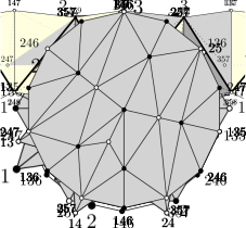
Figure 4: The construction of $\mathsf{QB}^{\bullet}(8,3)$. Top left: $\mathsf{QB}^{\bullet}_{1}(8,3)$. Top right: $\mathsf{QB}^{\circ}(6,2)$. Bottom: Filling in $\mathsf{QB}^{\bullet}_{1}(8,3)$ using $\mathsf{QB}^{\circ}(6,2)$ produces $\mathsf{QB}^{\bullet}(8,3)$. The labelling of the vertices inside the disk is discussed in rule (B9).

To relabel the vertices of $\mathsf{QB}^{\circ}(n-2,k-1)$ so as to accomplish step (B9), we will use the mapping $g_{n}$ of Section 3; recall that for $A\in V_{\,}(n-2,k-1)$,

$$g_{n}(A)=\begin{cases}(A+1)\cup\left\{{1}\right\}&\text{if $n-2\in A$,}\\ (A+1)\cup\left\{{n}\right\}&\text{otherwise.}\end{cases}$$

We relabel each black vertex $A^{\bullet}$ of $\mathsf{QB}^{\circ}(n-2,k-1)$ to $g_{n}(A)^{\bullet}$ (cf. Figure 4). A white vertex $A^{\circ}$ is relabelled to

$$g_{n}(A)^{\circ} A\in V_{+}(n-2,k-1)$$  if ,

$$g_{n-1}(A)^{\circ}$$  otherwise.

We need to check that any vertex at the interior boundary of $\mathsf{QB}^{\bullet}_{1}(n,k)$ is mapped to itself by $g_{n}\circ f$ ($g_{n-1}\circ f$, respectively). These are the vertices in the set $V_{\mathsf{IB}}$ defined in Lemma 10(i). Recall that

$$V_{\mathsf{IB}}=\bigcup_{A\in V_{+}(n-1,k)}\left\{{A\langle n\rangle^{\bullet},A^{\circ}}\right\}.$$

It follows from Lemma 5 that for $A\in V_{+}(n-1,k)$, $g_{n-1}(f(A))=A$ and $g_{n}(f(A\langle n\rangle))=A\langle n\rangle$, proving the requested property. Further properties of the labelling will be proved in Lemmas 12 and 14 below.

We finally construct $\mathsf{QK}(n,k)$ as follows:

1. We embed a deformed copy of $\mathsf{QB}^{\bullet}(n,k)$ in $\mathbb{R}^{n-2k+1}$, with its vertices placed in the closed upper hemisphere $H^{+}$ of $S^{n-2k}$, in such a way that the embedded complex is boundary-antisymmetric (thus, the boundary $\mathsf{QK}(n-1,k)$ is necessarily embedded in the ‘equator’ $S^{n-2k-1}$).

2. Projecting each vertex of $\mathsf{QB}^{\bullet}(n,k)$ to its antipode in $S^{n-2k}$ and inverting its colour, we obtain a copy of $\mathsf{QB}^{\circ}(n,k)$ in $H^{-}$ that matches the former copy at the boundary.

3. $\mathsf{QK}(n,k)$ is the result of glueing the two triangulated hemispheres together along their boundaries.

In several lemmas, we now verify the properties of $\mathsf{QK}(n,k)$ required by Theorem 8.

Lemma 12.

Each element of $V_{\,}(n,k)$ appears as (the label of) a vertex of $\mathsf{QK}(n,k)$.

Proof.

The assertion is easy to check for $n=2k+1$. If $n>2k+1$, we inductively assume that it is true for $n-1$. Thus, any set $A\in V_{\,}(n-1,k)$ is the label of a vertex of $\mathsf{QK}(n-1,k)\subseteq\mathsf{QK}(n,k)$.

By Lemma 3, it is sufficient to consider a set $A\in V_{+}(n,k)$. Let $B=f(A)$, where $B\in V_{\,}(n-2,k-1)$. By the induction hypothesis, $B$ is the label of a vertex of $\mathsf{QK}(n-2,k-1)$, and hence of the complex $\mathsf{QB}^{\circ}(n-2,k-1)$ used in the construction of $\mathsf{QB}^{\bullet}(n,k)$. We may assume that the vertex is $B^{\bullet}$ (the argument for $B^{\circ}$ being symmetric). The vertex was labelled with $g_{n}(B)$ in $\mathsf{QB}^{\bullet}(n,k)$; by Lemma 5(ii), $g_{n}(f(A))=A$ when $A\in V_{+}(n,k)$, so $A$ does appear as a vertex label in $\mathsf{QB}^{\bullet}(n,k)$ and $\mathsf{QK}(n,k)$. ∎

Lemma 13.

Any edge $A^{\bullet}B^{\circ}$ of $\mathsf{QB}^{\bullet}_{1}(n,k)$, where $A,B\in V_{\,}(n-1,k)$, is an edge of $\mathsf{QK}(n-1,k)$.

Proof.

Consider an edge $A^{\bullet}B^{\circ}$ of $\mathsf{QB}^{\bullet}_{1}(n,k)$ but not of $\mathsf{QK}(n-1,k)$, where $A,B\in V_{\,}(n-1,k)$. In the construction of $\mathsf{QB}^{\bullet}_{1}(n,k)$, which starts from $\mathsf{QK}(n-1,k)$, the edge $A^{\bullet}B^{\circ}$ was not added in steps (B1)–(B3) as these steps consist in adding clones of black vertices and contracting edges joining these clones. By Lemma 9(i), after step (B3) is completed, $A^{\bullet}$ is not contained in the interior boundary of the resulting complex $\mathsf{L}$. Consequently, steps (B4)–(B5) do not influence the set of edges incident with $A^{\bullet}$. Thus, there is no step where $A^{\bullet}B^{\circ}$ can be added, which is a contradiction. ∎

Lemma 14.

For any $A,B\in V_{\,}(n,k)$ such that $A^{\bullet}$ and $B^{\circ}$ are adjacent in $\mathsf{QK}(n,k)$, $A\cap B=\emptyset$.

Proof.

We proceed by induction on $n$. The claim is easy to verify for $n=2k+1$. Assume that this is not the case; in addition, we may assume that $k>1$. Let $A^{\bullet}B^{\circ}$ be an edge of $\mathsf{QK}(n,k)$.

Without loss of generality, $A^{\bullet}B^{\circ}$ is an edge of $\mathsf{QB}^{\bullet}(n,k)$ but not of $\mathsf{QK}(n-1,k)$. Suppose first that $A^{\bullet}B^{\circ}$ is an edge of $\mathsf{QB}^{\bullet}_{1}(n,k)$. By the fact that each white vertex of $\mathsf{QB}^{\bullet}_{1}(n,k)$ is a vertex of $\mathsf{QK}(n-1,k)$ and by Lemma 13, we find that $A^{\bullet}$ is not a vertex of $\mathsf{QK}(n-1,k)$. Inspecting steps (B1)–(B5) of the construction, we observe that there are two possibilities:

• there is a set $C\in V_{\,}(n-1,k)$ such that $A=C\langle n\rangle$ and $C^{\bullet}B^{\circ}$ is an edge of $\mathsf{QK}(n-1,k)$, or

• there are sets $C\in V_{\,}(n-1,k)$, $D\in V_{0}(n-1,k)$ such that $A=C\langle n\rangle$, $B=D\langle n-1\rangle$ and $C^{\bullet}D^{\circ}$ is an edge of $\mathsf{QK}(n-1,k)$.

In the first case, $C\cap B=\emptyset$ by the induction hypothesis and $n\notin C$, so $A\cap B=\emptyset$. In the second case, we similarly have $C\cap D=\emptyset$ by the induction hypothesis; since $n-1\notin A$ and $n\notin B$, we conclude $A\cap B=\emptyset$.

It remains to consider the case that the edge $A^{\bullet}B^{\circ}$ is not an edge of $\mathsf{QB}^{\bullet}_{1}(n,k)$. By the construction of $\mathsf{QB}^{\bullet}(n,k)$, $f(A)^{\bullet}f(B)^{\circ}$ is an edge of $\mathsf{QB}^{\circ}(n-2,k-1)$. By the induction hypothesis, $f(A)\cap f(B)=\emptyset$. By Lemma 5, since $A,B\in V_{+}(n,k)$, $A=g_{n}(f(A))$ and $B=g_{n}(f(B))$. The definition of $g_{n}$ shows that $A\cap B=\emptyset$ if one of $f(A)$, $f(B)$ contains $n-2$. Suppose thus that $n-2\notin f(A)\cup f(B)$. Then the $(n-2)$-level of both $f(A)$ and $f(B)$ is even. Since the vertices $f(A)^{\bullet}$ and $f(B)^{\circ}$ have different colours, the $(n-2)$-levels actually have to be zero by property (P1) of $\mathsf{QK}(n-2,k-1)$. Thus, $f(A),f(B)\in V_{0}(n-2,k-1)$, so $f(A)^{\bullet}f(B)^{\circ}$ is an edge of the exterior boundary $\mathsf{QK}(n-3,k-1)$ of $\mathsf{QB}^{\circ}(n-2,k-1)$ — but then $A^{\bullet}B^{\circ}$ would be an edge of the exterior boundary of $\mathsf{QB}^{\bullet}_{1}(n,k)$, a contradiction. ∎

Lemmas 12 and 14 imply part (iii) of Theorem 8. Parts (i) and (iv) follow easily from the construction. Part (ii) is a consequence of the following lemma:

Lemma 15.

The complex $\mathsf{QK}(n,k)$ contains no monochromatic maximal faces.

Proof.

The claim is certainly true for $\mathsf{QK}(2k+1,k)$. For $\mathsf{QK}(2k+2,k)$, it follows from the fact that each maximal face of $\mathsf{QB}^{\bullet}_{1}(2k+2,k)$ contains a $1$-dimensional face of either the exterior boundary or the interior boundary, and is therefore not monochromatic. With these base cases in hand, the lemma is proved by induction on $n$. Assume that $\mathsf{QK}(n-1,k)$ has no monochromatic maximal faces. The complex $\mathsf{QB}^{\bullet}_{1}(n,k)$ is obtained by two operations: adding clones and contracting $1$-dimensional monochromatic faces. None of these operations can create a monochromatic maximal face, so $\mathsf{QB}^{\bullet}_{1}(n,k)$ has no such faces. The rest follows using Lemma 10(ii) and induction. ∎

It only remains to check properties (P1)–(P3) of $\mathsf{QK}(n,k)$. This routine verification is left to the reader.

This concludes the proof of Theorem 8. We remark that the explicit construction of $\mathsf{QK}(2k+1,k)$ and $\mathsf{QB}^{\bullet}_{1}(2k+2,k)$ can, with minor modifications, be interpreted as a particular case of the general construction. Since a uniform treatment would make the exposition more complicated, we prefer to present these special cases separately.

Theorem 1 is a direct consequence of Theorem 8 and the results in [4]. Indeed, let the graph $QG(n,k)$ be obtained from the associated graph of $\mathsf{QK}(n,k)$ by identifying antipodal pairs of vertices (and discarding the colours). By Theorem 8 (i)–(ii) and [4, Lemma 3.2], $QG(n,k)$ is a quadrangulation of the projective space $\mathbb{P}^{n-2k}$. Theorem 8 (iii) implies that the quadrangulation is a spanning subgraph of $SG(n,k)$, while part (iv) implies that $QG(n,k)$ contains the $(2k+1)$-circuit $QG(2k+1,k)$ and is therefore non-bipartite. Finally, by [4, Theorem 1.1] and the easy upper bound on $\chi(SG(n,k))$, the chromatic number of $QG(n,k)$ is $n-2k+2$.

5 Conclusion

We conclude this paper with two open problems.

While the proof of Theorem 8 provides a recursive characterisation of the pairs of sets in $V_{\,}(n,k)$ that are adjacent in the graph $QG(n,k)$, it would be desirable to define this graph directly, without recursion. We have no such definition so far.

Recall that the Schrijver graph $SG(n,k)$ is a vertex-critical subgraph of the Kneser graph $KG(n,k)$ with the same chromatic number, namely $n-2k+2$. By Theorem 1, the spanning subgraph $QG(n,k)$ of $SG(n,k)$ has the same chromatic number, and we conjecture that it is the natural next step in the direction set by Schrijver:

Conjecture 16.

For any $k\geq 1$ and $n\geq 2k+1$, $QG(n,k)$ is edge-critical.

The conjecture is clearly true for $n=2k+1$ (odd cycles) and its validity for $n=2k+2$ can be derived from a result of Gimbel and Thomassen [1].

References

- [1] J. Gimbel and C. Thomassen. Coloring graphs with fixed genus and girth. Trans. Am. Math. Soc., 349:4555–4564, 1997.
- [2] A. Hatcher. Algebraic Topology. Cambridge University Press, Cambridge, 2002.
- [3] J. R. Munkres. Elements of Algebraic Topology. Addison–Wesley Publishing Company, Menlo Park, CA, 1984.
- [4] T. Kaiser and M. Stehlík. Colouring quadrangulations of projective spaces. J. Combin. Theory Ser. B, 113:1–17, 2015.
- [5] M. Kneser. Aufgabe 300. Jahresber. Deutsch., Math. Verein., 58:27, 1955.
- [6] L. Lovász. Kneser’s conjecture, chromatic number, and homotopy. J. Combin. Theory Ser. A, 25(3):319–324, 1978.
- [7] J. Matoušek. Using the Borsuk-Ulam theorem. Universitext. Springer-Verlag, Berlin, 2003.
- [8] A. Schrijver. Vertex-critical subgraphs of Kneser graphs. Nieuw Arch. Wisk. (3), 26(3):454–461, 1978.