Polarized thermal emission from X–ray Dim Isolated Neutron Stars: the case of RX J1856.5-3754

Abstract

The observed polarization properties of thermal radiation from isolated, cooling neutron stars depend on both the emission processes at the surface and the effects of the magnetized vacuum which surrounds the star. Here we investigate the polarized thermal emission from X–ray Dim Isolated Neutron Stars, taking RX J1856.5-3754 as a representative case. The physical conditions of the star outermost layers in these sources is still debated, and so we consider emission from a magnetized atmosphere and a condensed surface, accounting for the effects of vacuum polarization as the radiation propagates in the star magnetosphere. We have found that, for a significant range of viewing geometries, measurement of the phase-averaged polarization fraction and phase-averaged polarization angle at both optical and X–ray wavelengths allow us to determine whether this neutron star has an atmosphere or a condensed surface. Our results may therefore be relevant in view of future developments of soft X–ray polarimeters.

1 Introduction

X–ray dim isolated neutron stars (XDINSs), also known as the “Magnificent Seven”, are a class of isolated, radio-silent X–ray pulsars with peculiar properties, originally discovered by the ROSAT satellite (see e.g. Turolla, 2009, for a review). X–ray timing analysis allowed to measure the spin periods of all sources ($P\sim 3-12$ s; the latest addition being RX J1605.3+3249, $P=3.39$ s; Pires et al., 2014), together with the period derivatives, $\dot{P}\sim 10^{-14}-10^{-13}\rm{s~{}s}^{-1}$. These translate into spin-down magnetic fields $B\sim 10^{13}$ – $10^{14}$ G and characteristic ages $\tau_{c}$ of a few Myr. When available, kinematic age estimates based on the back-tracing of the star trajectory are typically shorter, $\sim 0.5$ Myr, and in agreement with those derived from the star cooling history (e.g. Mignani et al., 2013, and references therein).

XDINSs are quite close sources, possibly cradled in the young stellar clusters forming the Gould Belt Popov et al. (2003). The distances estimated from the hydrogen column density are $\la 500$ pc Posselt et al. (2008) and parallax measurements for RX J1856.5-3754 and RX J0720.4-3125 provide values of 123 and 360 pc, respectively (Walter et al., 2010; Kaplan & Van Kerkwijk, 2009, and references therein).

The Seven exhibit a purely thermal spectrum at X–ray energies with no evidence for a high-energy, power-law component often detected in other isolated NS classes. The X–ray luminosity is $10^{31}$ – $10^{32}\ {\rm erg\,s}^{-1}$, fully consistent with surface blackbody emission with temperatures $\sim 40$–100 eV and (radiation) radii of a few kilometers, as derived from X–ray spectral fits (see e.g. Kaplan & Van Kerkwijk, 2009; Turolla, 2009). With the only exception of RX J1856.5-3754, broad absorption features have been found in all XDINSs. These features have energies $\sim 300$ – 700 eV, equivalent widths of $\sim 50$ – 150 eV and, as in the case of RX J0720.4-3125, may be variable. In the latter source a second, strongly phase-dependent line was very recently reported Borghese et al. (2015).

Optical counterparts, with magnitudes $\ga 25$, have been identified (to a varying degree of confidence) for all the Seven on the basis of proper motion measurements or positional coincidence (e.g. Turolla, 2009; Kaplan et al., 2011). The optical flux appears to exceed the extrapolation of the X–ray blackbody at low energies by a factor $\sim 5$ – $50$ and deviations from a Rayleigh-Jeans distribution have been reported in some sources (notably RX J2143.0+0654; Kaplan et al., 2011).

The nature of the surface emission from XDINSs is still a debated issue. According to the conventional picture, isolated, cooling neutron stars are covered by an atmosphere which reprocesses the thermal radiation coming from the outermost stellar layers (see e.g. Potekhin, 2014, for a review). More recently, it has been appreciated that the low surface temperature ($\la 100\ {\rm eV}$) and the strong magnetic field ($\ga 10^{13}\ \rm G$) of XDINSs may produce a phase transition in the surface layers, leaving a bare neutron star with a condensed (either solid or liquid) surface (Lai & Salpeter, 1997; Lai, 2001; Burwitz et al., 2003; Turolla et al., 2004; Medin & Lai, 2007, see also Turolla 2009, Potekhin 2014).

The merits of the two models in explaining the observed multiwavelength spectral energy distribution (SED) of the XDINSs have been assessed in several studies, which are, however, hampered by the present poor knowledge of the star internal magnetic field structure and hence of the surface temperature distribution. Mid-Z element atmosphere models have been proposed for RX J1605.3+3249 Mori & Ho (2007). Pérez-Azorín et al. (2006) and Ho et al. (2007) used the condensed surface emission model to explain the observed properties of RX J0720.4-3125 and RX J1856.5-3754, respectively, although in the latter a thin, magnetized, H atmosphere on top of the condensate was added (as originally suggested by Motch, Zavlin & Haberl, 2003, see also Zane, Turolla & Drake 2004). A detailed, comparative investigation of atmospheric/condensed surface emission models was presented by Suleimanov et al. (2010), who also accounted for the possible presence of a thin H atmosphere around the condensed surface. Results were then applied to fit the SED of RX J1308.6+2127, showing that for this source an interpretation in terms of emission from a condensed surface with a thin atmosphere is favored Hambaryan et al. (2011).

Polarimetric measurements both at optical and X–ray energies can provide a valuable tool to better understand the physical properties of the neutron star surface. Current 8-m class telescopes, e.g. the VLT, already allow to perform polarization measures for faint sources like the XDINSs. X–ray polarimetry missions are at an advanced stage of development. The X–ray Imaging Polarimetry Explorer(XIPE), the Imaging X–ray Polarimetry Explorer(IXPE), and the Polarimeter for Relativistic Astrophysical X–ray Sources(PRAXyS) have been selected for the study phase of the ESA M4 and the NASA SMEX programmes. They will open the possibility to perform X–ray polarimetry and pave the way toward the construction of a X–ray polarimeter efficient in the soft X–rays.

Radiation from the surface of a neutron star is expected to be intrinsically polarized, because the strong magnetic field introduces an anisotropy in the medium in which electromagnetic waves are propagating. This, in turn, causes the opacity of the two normal modes (the ordinary and extraordinary) to be different, so that the emergent radiation carries a net polarization (see e.g. Harding & Lai, 2006). The expected polarization pattern is different whether emission comes from an atmosphere van Adelsberg & Lai (2006) or a condensed surface Potekhin et al. (2012). Thus, the study of the polarized emission from XDINSs can give us insight about the nature of the surface of strongly magnetized NS and ultimately probe the properties of the matter under strong magnetic fields.

Among the “Magnificent Seven”, the most promising source for the study of polarized emission in the optical and X-ray band is RX J1856.5-3754 (hereafter RX J1856). This is the brightest and nearest XDINS, with $V=25.58$, a nearly $\lambda^{-4}$ optical-UV SED van Kerkwijk & Kulkarni (2001); Kaplan et al. (2011) and a X–ray spectrum well modeled by two blackbody components ($T^{\infty}_{\mathrm{c}}\sim 40$ eV and $T^{\infty}_{\mathrm{h}}\sim 60$ eV; Sartore et al., 2012). The period derivative of RX J1856 has been obtained by van Kerkwijk & Kaplan (2008), $\dot{P}\sim 3\times 10^{-14}\ {\rm s/s}$, which translates into a spin-down magnetic field of $B\sim 1.5\times 10^{13}$ G. An alternative estimate, $B_{p}=6\times 10^{12}$ G (at the magnetic pole, assuming a dipole model), has been derived from fitting continuum models to the observed optical and X-ray spectrum (Ho et al., 2007). These relatively strong magnetic fields imply that a non vanishing degree of polarization is indeed expected in the thermal emission of the source.

In this paper we derive expectations for the polarization observables, focusing on the case of RX J1856. First, we briefly summarize the theoretical brackground to calculate the thermal emission from a magnetized atmosphere and a condensed surface (§ 2). Then, we proceed to the calculation of the intrinsic polarization properties (i.e. those at the star surface) for a magnetized, fully-ionized H atmosphere and for a condensed surface (§ 3.1). We then turn to the evaluation of the polarization fraction and the polarizations angle as measured by a distant observer, accounting for the effects of QED (vacuum polarization) and of the non-uniform star magnetic field (§ 3.2); this is done following closely the approach described in Taverna et al. (2015, hereafter paper I). Results are presented in § 4. Discussion and conclusions follow in § 5.

2 Theoretical framework

In this section we briefly outline the basic physical inputs of our model. Since XDINSs are slow rotators ($P\sim$ a few seconds, Turolla 2009), we neglect the effects of rotation and assume that the space-time outside the star is described by the vacuum Schwarzschild solution. Moreover, despite our treatment can handle general axially-symmetric magnetic fields, in the following we restrict to the case in which the neutron star field is dipolar, $\mathbf{B}=B_{\mathrm{p}}=(R_{\mathrm{NS}}/r)^{3}(f_{\mathrm{dip}}\cos\theta,g_{\mathrm{dip}}\sin\theta/2,0)$, where $B_{\mathrm{p}}$ is the polar field strength, $R_{\mathrm{NS}}$ is the star radius ($M_{\mathrm{NS}}$ denotes the star mass) and $r$, $\theta$ are the radial coordinate and the magnetic co-latitude, respectively. The two functions

$$\begin{array}[]{l}f_{\mathrm{dip}}=-\dfrac{3}{x^{3}}\left[\ln(1-x)+\dfrac{1}{2}x(x+2)\right]\\ g_{\mathrm{dip}}=\sqrt{1-x}\left(-2f_{\mathrm{dip}}+\dfrac{3}{1-x}\right)\,,\end{array}$$ (3)

account for relativistic corrections Ginzburg & Ozernoi (1965); Muslimov & Tsygan (1985), with $x=R_{\mathrm{s}}/r$, and $R_{\mathrm{s}}=2GM_{\mathrm{NS}}/c^{2}$.

2.1 Ray tracing method

Given an emission model characterized by a specific intensity $I_{\nu}$, which in general depends on the photon frequency $\nu$ and direction $\mathbf{k}$, and on the position on the star surface, the spectral and polarization properties at infinity are computed by summing the contributions of the surface elements which are into view at a given rotational phase.

Following Zane & Turolla (2006) and paper I, we introduce the two angles $\chi$ and $\xi$: the former is the angle between the line-of-sight (LOS, unit vector $\boldsymbol{\ell}$) and the spin axis ($\mathbf{p}$), while the latter is that between the magnetic (dipole) axis ($\mathbf{b}_{\rm dip}$), and the spin axis. We further introduce a (fixed) coordinate system, $(X,Y,Z)$ with the $Z$-axis parallel to $\boldsymbol{\ell}$ (i.e. along the LOS) and the $X$-axis in the $(\boldsymbol{\ell},\mathbf{p})$ plane, and a co-rotating coordinate system, $(x,y,z)$, with the $z$-axis parallel to $\mathbf{b}_{\rm dip}$ and the $x$-axis defined below. The associated polar angles are $(\Theta_{\mathrm{S}},\Phi_{\mathrm{S}})$ and $(\theta,\phi)$, respectively. In the fixed frame, the cartesian components of $\mathbf{p}$ and $\mathbf{b}_{\rm dip}$ are $\mathbf{p}=(\sin\chi,0,\cos\chi)$ and $\mathbf{b}_{\rm dip}=(\sin\chi\cos\xi-\cos\chi\sin\xi\cos\gamma,\sin\xi\sin\gamma,\cos\chi\cos\xi+\sin\chi\sin\xi\cos\gamma)$, where $\gamma=\omega t$ is the phase angle ($\omega=2\pi/P$, and $P$ is the star rotational period). We also define an additional vector, $\mathbf{q}=(-\cos\chi\cos\gamma,\sin\gamma,\sin\chi\cos\gamma)$, which is a unit vector orthogonal to $\mathbf{p}$ and rotating with angular velocity $\omega$ (in the fixed frame). The $x$-axis of the rotating coordinate system is then chosen in the direction of the component of $\mathbf{q}$ perpendicular to $\mathbf{b}_{\rm dip}$,

$$\mathbf{q}_{\perp}=\frac{\mathbf{q}-(\mathbf{b}_{\rm dip}\cdot\mathbf{q})\mathbf{b}_{\rm dip}}{\left[1-(\mathbf{b}_{\rm dip}\cdot\mathbf{q})^{2})\right]^{1/2}}\,.$$ (4)

The transformations linking the pairs of polar angles in the two systems are (see Zane & Turolla, 2006, paper I)

$$\cos\theta = \mathbf{b}_{\rm dip}\cdot\mathbf{n}$$

$$\cos\phi = \mathbf{n}_{\perp}\cdot\mathbf{q}_{\perp}$$ (5)

where $\mathbf{n}=(\sin\Theta_{\mathrm{S}}\cos\Phi_{\mathrm{S}},\sin\Theta_{\mathrm{S}}\sin\Phi_{\mathrm{S}},\cos\Theta_{\mathrm{S}})$ is the radial unit vector in the fixed coordinate system and $\mathbf{n}_{\perp}$ is defined in analogy with $\mathbf{q}_{\perp}$. Equations (2.1) are needed to express the intensity, which is naturally written in terms of the magnetic coordinate angles $(\theta\,,\phi)$, see §2.2, 2.3, in terms of the polar angles of the fixed frame $(\Theta_{\mathrm{S}}\,,\Phi_{\mathrm{S}})$ over which integration is performed.

At each phase the monochromatic flux detected by an observer at distance $D\gg R_{\mathrm{NS}}$ is obtained by integrating the intensity (in the fixed coordinate system) over the visible part of the surface (see e.g. Page, 1995; Zane & Turolla, 2006, paper I)

$$F_{\nu}(\gamma)=\left(1-\frac{R_{\mathrm{s}}}{R_{\mathrm{NS}}}\right)\frac{R_{\mathrm{NS}}^{2}}{D^{2}}\int_{0}^{2\pi}d\Phi_{\mathrm{S}}\int_{0}^{1}I_{\nu}(\mathbf{k},\theta,\phi)du^{2}\,,$$ (6)

where $u=\sin\bar{\Theta}$. The two angles, $\Theta_{\mathrm{S}}$ and $\bar{\Theta}$, are related by the “ray tracing” integral

$$\bar{\Theta}=\int_{0}^{1/2}dv\,\sin\Theta_{\mathrm{S}}\left[\frac{1}{4}(1-x)-(1-2vx)v^{2}\sin\Theta_{\mathrm{S}}^{2}\right]^{-1/2}\,.$$ (7)

For $x\ll 1$ Newtonian geometry is recovered and $\bar{\Theta}=\Theta_{\mathrm{S}}$. A $50\times 50$ mesh in $\cos\Theta_{\mathrm{S}}$ and $\Phi_{\mathrm{S}}$, equally spaced in the $[0,1]$ and $[0,2\pi]$ intervals, respectively, is typically used in our numerical calculations.

In the case of radiation (linearly) polarized in the two normal modes (the ordinary, O, and the extraordinary, X, mode), the total intensity is just the sum of the intensities in the two modes

$$I_{\nu}(\mathbf{k},\theta,\phi)=I_{\nu,\mathrm{O}}(\mathbf{k},\theta,\phi)+I_{\nu,\mathrm{X}}(\mathbf{k},\theta,\phi)$$ (8)

and we define the “intrinsic” degree of polarization, i.e. that at the source, as

$$\Pi_{\mathrm{L}}^{\mathrm{EM}}=\frac{F_{\mathrm{X}}-F_{\mathrm{O}}}{F_{\mathrm{X}}+F_{\mathrm{O}}}\,,$$ (9)

where $F_{\mathrm{X,O}}$ is the monochromatic, phase-dependent flux in each mode, defined as in equation (6).

Figure 1: Degree of polarization for emission from a pure H ionized atmosphere with $T=10^{6.5}$ K and magnetic field perpendicular to the surface. The solid line corresponds to $B=10^{12}$ G, and the dotted line to $B=10^{13}$ G. See text for details.

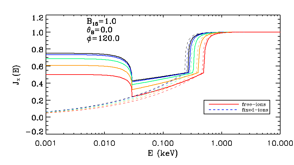
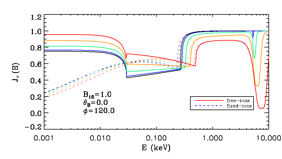
Figure 2: The condensed-surface emissivity in the X (left) and O mode (right). Full (dashed) lines refer to the free (fixed)-ions approximation. The different colours are for different values of $\theta_{\mathrm{k}}$ ($0^{\circ}$, black; $15^{\circ}$, blue; $30^{\circ}$, green; $45^{\circ}$, orange; $60^{\circ}$, red). Here $\phi_{\mathrm{k}}=120^{\circ}$, $\theta_{\mathrm{B}}=0$ and $B=10^{13}$ G.

2.2 Atmosphere

Atmospheres around cooling NSs are commonly modeled by considering a gas in radiative and hydrostatic equilibrium. Since the scaleheight of the atmosphere, $h\sim kT/m_{p}g\sim 10$ cm, is much smaller than the star radius, the radiative transfer equation is solved in the plane-parallel approximation, usually assuming an atmosphere in local thermodynamic equilibrium. Atmospheric models have been presented by a number of authors, under different assumptions and accounting for different degrees of sophistication in the description of radiative processes and the plasma composition (see e.g. Potekhin, 2014, for a review). Our objective in this work is to derive simple expectations for the difference in the polarization signal emitted in the case the NS is covered by a gaseous layer or it is “bare” (see § 2.3). We therefore adopt the assumption that of a fully ionized pure H atmosphere and avoid the complication of atmospheric compositions. The emergent intensity is computed using the numerical method presented in Lloyd (2003, see also ). The code exploits a complete linearization technique for solving the stationary radiative transfer equations for the two normal polarization modes in a plane-parallel slab, by including the effect of the magnetic field inclination with respect to the surface normal. The source term accounts for magnetic bremsstrahlung and magnetic Thompson scattering.

The spectral calculations have four input parameters: the (local) effective temperature $T$ and magnetic field strength, $B$, the angle between the local magnetic field $\mathbf{B}$ and the surface normal $\mathbf{n}$, $\theta_{\mathrm{B}}$, and the surface gravity, $g$. The code solves for the emergent intensity $I_{\nu}(\mathbf{k})\equiv I(E,\mu_{\mathrm{k}},\phi_{\mathrm{k}})$ for a range of photon energies $E=h\nu$, photon co-latitudes and azimuthal angles relative to the slab normal, $\theta_{\mathrm{k}}=\arccos(\mu_{\mathrm{k}})$ and $\phi_{\mathrm{k}}$, respectively. The $\phi_{\mathrm{k}}=0$ direction is defined by the projection of the magnetic field on the symmetry planes. We should notice that, since the magnetic field introduces an anisotropy in the opacities, the emergent intensity is not symmetric with respect to a rotation around the surface normal but instead it depends on both, $\mu_{\mathrm{k}}$ and $\phi_{\mathrm{k}}$. For the particular case in which $\theta_{\mathrm{B}}=0$, symmetry with respect to $\phi_{\mathrm{k}}$ is restored, so the calculation is restricted to the $\mu_{\mathrm{k}}$-dependent intensities. Moreover, even in the general case $\theta_{\mathrm{B}}>0$, thanks to the symmetry properties of the opacities, the calculation of the emergent spectrum can be restricted to $0<\phi_{\mathrm{k}}<\pi$.

Since we are considering photon energies well below the electron cyclotron frequency, the opacity for O-mode photons is almost unaffected by the magnetic field, while that for X-mode ones is substantially reduced (Harding & Lai, 2006). Therefore, in general, the emergent intensity of the X-mode is much larger than that of the O-mode, resulting in an emergent radiation with a non-null degree of polarization. This is illustrated in Figure 1, that shows the intrinsic polarization fraction, as a function of the energy, for a single model, assuming a parallel magnetic field ($\theta_{\mathrm{B}}=0$). As it can be seen, for $B=10^{13}$ G, the polarization fraction is relatively high in the optical band ($\sim 70\%$) and it tends to increase at high energies.

Figure 3: Pure H, fully ionized atmosphere model for the emission from RX J1856. The dotted line correspond to the the X–ray lightcurve (LC), while the solid and dashed lines correspond to the phase dependent polarization fraction in the X–ray band and in the optical band, respectively. The viewing geometry is such that $\chi=90^{\circ}$ and $\xi=15^{\circ}$. See text for details.

2.3 Condensed surface

Magnetic fields higher than $\sim m_{e}^{2}e^{3}c/\hbar^{3}=2.4\times 10^{9}\ \mathrm{G}$ change the properties of atoms, confining electrons in the direction perpendicular to the magnetic field. These elongated, cylindrical atoms can form molecular chains by covalent bonding along the magnetic field lines. In turn, chain-chain interaction can lead to the formation of a condensed phase, as originally suggested by Lai & Salpeter (1997, see also ). The cohesive energy for linear chains increases with the magnetic field strength and it is expected that, for sufficiently strong magnetic fields, there is a critical temperature, $T_{\mathrm{crit}}$, below which a phase transition between a gaseous and a condensed state occurs. This critical temperature depends on composition and increases with magnetic field strength Lai (2001); Medin & Lai (2007). Most recent estimates give $T_{\mathrm{crit}}\approx 10^{5}[5+2(B/10^{13}\ \rm G)]$ K for Fe composition, meaning that a phase transition may occur for surface temperatures $T\ga 10^{6}$ K if the field is stronger than $\sim 10^{13}\ \rm G$. Since these are the typical surface temperature and magnetic field found in XDINSs, the thermal spectrum may indeed come from a condensed surface Turolla et al. (2004).

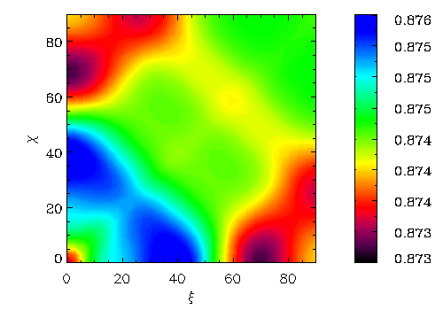
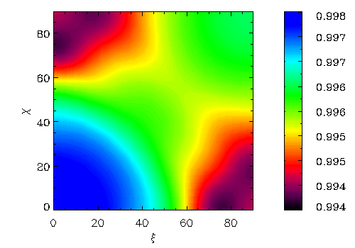
Figure 4: Contour plots of the intrinsic, phase-average polarization fraction in the ($\chi$, $\xi$) plane for the gaseous atmosphere model, with the left panel for the optical (B-filter) band and the right panel for the X–ray (0.12 - 0.39 keV, at infinity) band. See text for details.

The spectral properties of emission from a neutron star with a condensed surface were investigated in several papers since the pioneering work of Brinkmann (1980). In essence, the intensity is computed from the emissivity coefficient, $j_{\nu}$, which is in turn related to the reflectivity via Kirchhoff’s law. The latter is calculated applying Snell’s law at the interface between the vacuum and the condensed phase. The boundary conditions for the transmission of an electromagnetic wave across the two media give the amplitude of the reflected waves (Turolla et al., 2004; Pérez-Azorín et al., 2005; van Adelsberg et al., 2005; Suleimanov et al., 2010, see also Potekhin 2014).

There are uncertainties in this kind of calculation. Our present knowledge of the condensate is poor, and the lacking of a reliable expression of the dielectric tensor hinders the correct derivation of the reflectivity. Previous works adopted a simplified treatment, in which only the limits of “free ions” (no account for the effects of the lattice on the interaction of the electromagnetic waves with ions) and of “fixed ions” (no ion response to the electromagnetic wave because lattice interactions are dominant) were considered. The true reflectivity of the surface is expected to lie in between these two limits.

Here we maintain the same approach and use the analytical approximations by Potekhin et al. (2012) to compute the emissivities in the two normal modes. They depend on the magnetic field $B$, the photon direction $\mathbf{k}$ and energy, and the angle between $\mathbf{k}$ and $\mathbf{B}$, $\theta_{\mathrm{Bk}}$. However, the modes $1,\,2$ of Potekhin et al. (2012) are not defined with respect to the local direction of $\mathbf{B}$ but with respect to the local normal $\mathbf{n}$, with mode 1 perpendicular to both $\mathbf{k}$ and $\mathbf{n}$. As a consequence, the emissivities $j_{\nu,\mathrm{i}}$ ($\mathrm{i}=1,\,2$) do not coincide with those in the X and O modes, unless $\mathbf{n}$ and $\mathbf{B}$ are parallel, i.e. $\theta_{\mathrm{B}}=0$. The transformation linking the emissivities in the two basis is given in Appendix B of Potekhin et al. (2012). Once the transformation is perfomed the intensity of the emergent radiation in the X and O modes follows, by assuming the radiance of a blackbody, $B_{\nu}(T)=2h\nu^{3}/[c^{2}(\exp{(h\nu/kT)}-1)]$,

$$I_{\nu,\mathrm{O}}=j_{\nu,\mathrm{O}}(\nu,B,\mathbf{k},\theta_{\mathrm{Bk}})B_{\nu}(T)$$

$$I_{\nu,\mathrm{X}}=j_{\nu,\mathrm{X}}(\nu,B,\mathbf{k},\theta_{\mathrm{Bk}})B_{\nu}(T)\,.$$ (10)

Figure 2 shows the emissivity in the two normal modes, calculated in the two limits (“free” and “fixed” ions), for different values of $\theta_{\mathrm{k}}$.

3 The model for RX J1856

Figure 5: Same as in Figure 3 for the condensed surface. The dotted line is the X–ray lightcurve, while the solid and dashed lines are the phase dependent polarization degree in the X–ray and in the optical band, respectively. Thick curves correspond to free ions, and thin curves to fixed ions. Note that the X–ray lightcurve and phase dependent polarization degree in the optical band are almost indistinguishable in the two cases. Here $\chi=90^{\circ}$ and $\xi\approx 18^{\circ}$. See text for details.

In the following we consider a NS with mass $M_{\mathrm{NS}}=1.5~{}M_{\odot}$ and radius $R_{\mathrm{NS}}=12$ km, which is compatible with expectations from modern equations of state such as APR or BSk21 models (Akmal et al., 1998; Goriely et al., 2010). The value of the radius is also in agreement with the estimates derived by Sartore et al. (2012) and Ho et al. (2007), assuming a source distance of 120 pc (Walter et al., 2010). This choice translates into a gravitational red-shift factor at the star surface $1+z=1.26$. The rotational period of RX J1856 is $P=7$ s and the X–ray pulsed fraction is the lowest among the XDINSs, $\sim 1.3\%$ Tiengo & Mereghetti (2007). The polar strength of the dipole field is taken to be $B_{\mathrm{p}}=10^{13}$ G, a value which is somehow intermediate between the spin-down measure and the estimates from spectral fitting (van Kerkwijk & Kaplan, 2008; Ho et al., 2007). We assume that the magnetic field is dipolar (see §2) and that the surface temperature distribution is that induced by the core-centered dipole. Since for fields higher than $\sim 10^{11}\ \mathrm{G}$, electron conduction across the field lines is strongly suppressed, the meridional temperature variation is $T_{\mathrm{dip}}\simeq T_{\mathrm{p}}|\cos\theta_{\mathrm{B}}|^{1/2}$, where $T_{\mathrm{p}}$ is the polar value of the temperature (e.g. Greenstein & Hartke, 1983). We checked that this simple expression for $T_{\mathrm{d}ip}$ differs only slightly ($\la 6\%$) from the more accurate formula by Potekhin et al. (2015) for $\theta\la 80^{\circ}$. However, taken face value, the previous expression for $T_{\mathrm{dip}}$ yields vanishingly small values near the magnetic equator. The analysis of Sartore et al. (2012) has shown that the X–ray spectrum of RX J1856 is best modeled in terms of two blackbody components with $kT^{\infty}_{\mathrm{h}}\sim 60$ eV and $kT^{\infty}_{\mathrm{c}}\sim 40$ eV. To account for this in a simple way, we actually adopt a temperature profile given by $T_{\mathrm{s}}=\max(T_{\mathrm{dip}},T_{\mathrm{c}})$ with $T_{\mathrm{p}}=T_{\mathrm{h}}$, where $T_{\mathrm{h,c}}=T^{\infty}_{\mathrm{h,c}}/(1+z)$.

3.1 Intrinsic polarization degree

3.1.1 Atmosphere

We first consider the case in which the star is surrounded by a gaseous atmosphere. The star surface is divided in six angular patches in magnetic colatitude, centered at the values $\theta=\{0^{\circ},10^{\circ},30^{\circ},50^{\circ},70^{\circ},89^{\circ}\}$. By using the magnetic and temperature profiles previously described we compute, for each $\theta$, the local magnetic field strength, $B$, the angle $\theta_{\mathrm{B}}$ between the magnetic field and the normal to the surface, and hence the temperature, $T$. We then compute a set of atmospheric models corresponding to the six $\theta$ angles. Since the models are computed using different integration grids in the photon phase space (because the choice of the photon trajectories along which the radiative transfer is solved needs to be optimized to ensure fast convergence at the different values of magnetic field strength and inclination, see Lloyd, 2003), we reinterpolate all model outputs over a common grid. This results in three 4-D arrays for the emergent intensity $I^{i}_{\nu}(\mathbf{k},\theta)\equiv I^{i}(E,\mu_{k},\phi_{k},\theta)$ ($i=1,...3$) which contain the total intensity and the intensities for the ordinary and extraordinary modes, respectively. In order to take into account the emission from the southern magnetic hemisphere of the star, we use the previous 4-D arrays with the substitutions $\theta_{B}\rightarrow\pi-\theta_{B}$ and $\phi_{k}\rightarrow\pi-\phi_{k}$, which is justified by the simmetry properties of the opacities. By using the ray tracing method described in § 2, we can then compute lightcurves, phase resolved spectra and polarization fractions for each choice of the angles $\chi$ and $\xi$. As an example, Figure 3 shows the X–ray lightcurve ($0.12-0.39$ keV) and the phase–dependent polarization degree in the X–ray and optical (B–filter) bands, for $\chi=90^{\circ}$ and $\xi=15^{\circ}$. For this particular viewing geometry, the X–ray pulsed fraction is $1\%$, in agreement with the observed data and, as illustrated in the figure, the polarization degree is expected to be substantial and constant in phase.

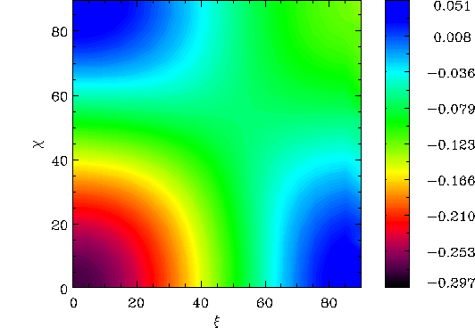
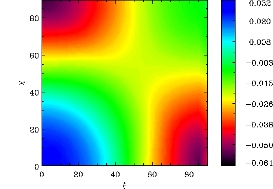
Figure 6: Contour plots of the intrinsic, phase-average polarization fraction in the ($\chi$, $\xi$) plane for the free-ion crustal emission model, with the left panel for the optical (B-filter) band and the right panel for the X–ray (0.12 - 0.39 keV) band.

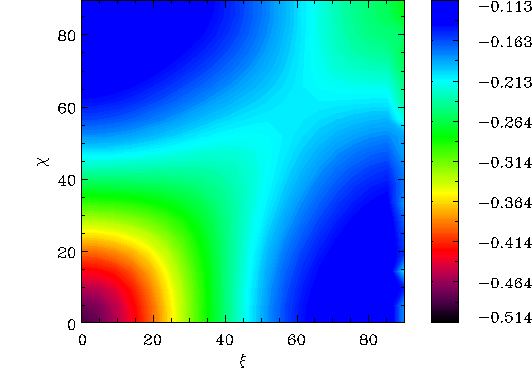
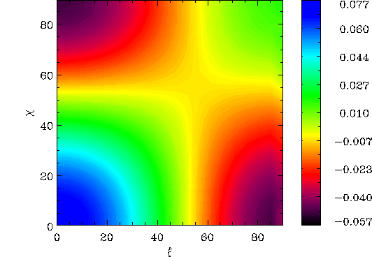
Figure 7: Same as in Figure 6 but for the fixed-ion crustal emission model.

Figure 4 shows the contour plots of the phase-averaged polarization fraction in the ($\chi$, $\xi$) plane, for the X–ray ($0.12-0.39$ keV) and optical (B-filter) bands. In both cases the phase-averaged polarization degree is significantly high. Like the results already obtained for the viewing geometry used in Figure 3, the phase-averaged polarization degree in the X–ray band is $\sim 99\%$, and that in the optical band is only slightly lower, $\sim 87\%$.

It is important to stress that these plots (and the analogous ones in §3.1.2) show the polarization degree as computed by using the definition given in equation (9), i.e. considering the difference in the radiative flux carried by the two modes when radiation reaches infinity, and repeating the calculation at different spin phases. Although we take into account for relativistic ray bending (i.e. for the fact that the emitting area which is into view is larger than a hemisphere), a proper calculation of the polarization observables is based on the Stokes parameters and must account for both QED effects in the magnetized vacuum through which photons propagate and the rotation of the plane normal to the photon wavevector in a varying magnetic field (see §3.2), effects that are not accounted for in the plots of Figure 4. We therefore refer to this quantity as the “intrinsic” degree of linear polarization, to distinguish it from the observed one, which is discussed later on (see section 4). We remark that both the “intrinsic” and the observed degree of polarization are evaluated at infinity, and a comparison of the two quantities may be of help in understanding how QED and geometrical effects influence the polarization observables.

3.1.2 Condensed surface

The same approach described in the previous subsection was used to compute the (phase-dependent) spectrum and the intrinsic polarization fraction for a bare INSs with a condensed surface. In this case the calculation was repeated twice, by assuming either “free” or “fixed” ions. Since we adopt the approximated analytical expressions by Potekhin et al. (2012) for the emissivities, no interpolations were required, contrary to the case of the atmosphere. The fitting formulae, however, cover the range $0\leq\theta_{\mathrm{B}}\leq\pi/2$. In order to take into account the emission from the southern magnetic hemisphere of the star, where $\mathbf{B}$ “enters” into the surface and $\pi/2<\theta_{\mathrm{B}}\leq\pi$, the emissivities are calculated by replacing $\cos\theta_{\mathrm{B}}$ with $-\cos\theta_{\mathrm{B}}$ and $\cos\phi_{\mathrm{k}}$ with $-\cos\phi_{\mathrm{k}}$ (A. Potekhin, private communication). Results are reported in Figure 5, where the X–ray lightcurve and the phase dependent polarization degree are shown for $\chi=90^{\circ}$ and $\xi\sim 18^{\circ}$, which is again compatible with a pulsed fraction of $\sim 1\%$. The corresponding contour plots for the X–ray and optical phase-averaged polarization fraction are shown in Figure 6 (free ions) and Figure 7 (fixed ions), respectively. In the case of free ions, the phase-averaged polarization degree in the X–ray band is always less than $\sim 6\%$ either when the emission is dominated by ordinary (negative values) or extraordinary photons (positive values, see Figure 6, right panel), while in the optical band (Figure 6, left panel) ordinary photons are predominant, with a maximum polarization degree $\sim 30\%$ for particular viewing geometries. In the case of fixed ions expectations are similar in the X–ray band, where the phase-averaged polarization degree is always less than $\sim 8\%$. However, in the optical band, the polarization degree can be slightly larger, up to $\sim 50\%$ (Figure 7, left panel), for the most favorable viewing geometries.

3.2 Stokes parameters and vacuum polarization

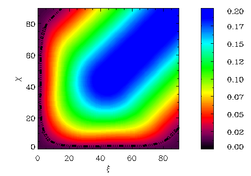
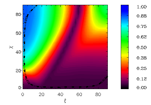
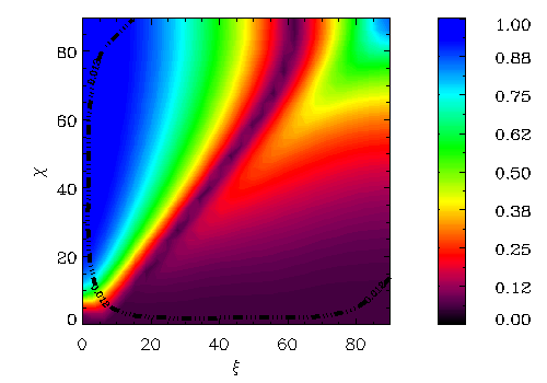
Figure 8: Contour plots for the X–ray pulsed fraction, phase-averaged polarization fraction in the optical (B filter) band and phase-averaged polarization fraction in the X–ray band in the ($\chi$,$\xi$) planes (panels from left to right respectively) for the gaseous atmosphere model. All polarization observables are computed by the expressions of the Stokes parameters (see § 3.2). The black curve in each panel corresponds to the observed X–ray pulsed fraction of RX J1856, $\sim 1\%$.

A strong magnetic field can modify the properties of the vacuum outside the NS. In particular, due to QED effects, photons can temporarily convert into electron-positron pairs, and those virtual pairs modify the dielectric and the magnetic permeability tensors of the vacuum. This affects the direction of the photon electric field and, in turn, influences the polarization fraction as observed at infinity (Heyl & Shaviv, 2000, 2002, see also Harding & Lai 2006). As a linearly polarized electromagnetic wave propagates in the magnetized vacuum close to the star, the direction of the electric field changes on a spatial scale much shorter than that over which $\mathbf{B}$ varies. This implies that up to the adiabatic (or polarization-limiting) radius

$$r_{\mathrm{a}}\simeq 4.8\left(\frac{B_{\mathrm{p}}}{10^{11}\ \mathrm{G}}\right)^{2/5}\left(\frac{E}{1\ \mathrm{keV}}\right)^{1/5}R_{\mathrm{NS}}\,,$$ (11)

a photon will keep the polarization mode (either X or O) in which it was emitted. Around $r_{\mathrm{a}}$, the coupling between $\mathbf{B}$ and the wave electric field weakens, until for $r\gg r_{\mathrm{a}}$, the direction of the electric field freezes (Heyl, Shaviv & Lloyd, 2003; Fernández & Davis, 2011, paper I).

The evolution of the wave electric field can be followed by solving the (linearized) wave equation in the magnetized vacuum around the star along each photon trajectory. However, as shown in paper I, the main effects of vacuum polarization can be cought using a simpler approach in which adiabatic propagation (i.e. mode locking) is assumed up to $r_{\mathrm{a}}$, while the electric field direction is constant (and modes change) for $r>r_{\mathrm{a}}$. In this approach the polarization properties are determined by the direction of the magnetic field at $r_{\mathrm{a}}$, in addition to the intrinsic polarization degree at the surface.

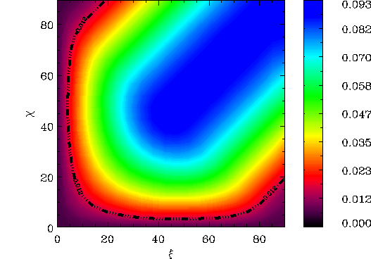
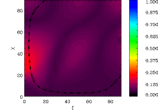
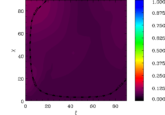
Figure 9: Same as Figure 8 but for the free-ion crustal emission model.

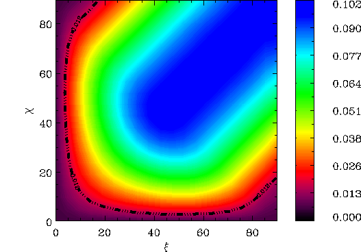
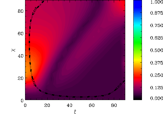
Figure 10: Same as Figure 8 but for the fixed-ion crustal emission model.

Since the X and O modes are defined according to the direction of the wave electric field with respect to the plane spanned by the magnetic field $\mathbf{B}$ and the wavevector $\mathbf{k}$, the Stokes parameters of photons crossing $r_{\mathrm{a}}$ at different positions are, in general, referred to different coordinate systems. While the $z_{i}^{\prime}$ axes coincide with the LOS (i.e. with $\boldsymbol{\ell}$), the two axes, $x_{i}^{\prime},\,y_{i}^{\prime}$, in the plane orthogonal to $\boldsymbol{\ell}$ will be different for each photon trajectory, because $\mathbf{B}$ changes its direction over the sphere of radius $r_{\mathrm{a}}$. In order to derive the polarization observables, as detected by a distant instrument, the Stokes parameters must be referred to the same fixed direction in the plane perpendicular to the LOS, $\mathbf{u}$. This is done by rotating the Stokes parameters by an angle $\alpha_{i}=\arccos\mathbf{u}\cdot{\mathbf{x}}_{i}$ (for the choice of the sign of $\alpha_{i}$ see, Paper I)

$$I_{i} = \bar{I}_{i}$$

$$Q_{i} = \bar{Q}_{i}\cos(2\alpha_{i})+\bar{U}_{i}\sin(2\alpha_{i})$$ (12)

$$U_{i} = \bar{U}_{i}\cos(2\alpha_{i})-\bar{Q}_{i}\sin(2\alpha_{i})\,.$$

In a strong magnetic field, each photon is 100$\%$ polarized either in the X-mode or O-mode. This is conveniently expressed in terms of the (normalized) Stokes parameters of each photon as $\bar{I}_{i}=1$, $\bar{Q}_{i}=\pm 1$ (for X-mode and O-mode photons) and $\bar{U}_{i}=0$ (see paper I). The collective Stokes parameters, i.e. those for the entire radiation field, are simply the sum of the individual parameters. This is immediately generalized to a continuum photon distribution following the same approach as in equation (6)

$$I = \int_{0}^{2\pi}d\Phi_{\mathrm{s}}\int_{0}^{1}du^{2}(n_{\mathrm{X}}+n_{\mathrm{O}})$$

$$Q = \int_{0}^{2\pi}d\Phi_{\mathrm{s}}\int_{0}^{1}du^{2}(n_{\mathrm{X}}-n_{\mathrm{O}})\cos(2\alpha)$$ (13)

$$U = \int_{0}^{2\pi}d\Phi_{\mathrm{s}}\int_{0}^{1}du^{2}(n_{\mathrm{O}}-n_{\mathrm{X}})\sin(2\alpha)\,,$$

where $n_{\mathrm{O,X}}=I_{\mathrm{O,X}}/E$, and $Q,\,U$ are the fluxes of the Stokes parameters; here $I$ is proportional to the total number flux and in (3.2) the constant factor appearing in front of the integral (see equation [6]) has been dropped. The explicit expression for $\alpha$ as a function of $\Theta_{\mathrm{s}}$, $\Phi_{\mathrm{s}}$, $\xi$, $\chi$, the phase $\gamma$ and the photon energy, $E$ was derived in paper I. Finally, the observed polarization fraction and polarization angle are given by the usual expressions

$$\Pi_{\mathrm{L}} = \frac{\sqrt{Q^{2}+U^{2}}}{I}$$ (14)

$$\chi_{\mathrm{P}} = \frac{1}{2}\arctan\left(\frac{U}{Q}\right)\,.$$ (15)

4 The observed polarization signal

With the method described in § 3.2, we can determine the polarization of the radiation as measured by a distant observer for any given viewing configuration. In particular, we compute and compare the X–ray pulsed fraction, the phase-averaged degree of polarization and polarization angle in the X–ray and in the optical bands as functions of the two geometrical angles $\chi$ and $\xi$. Here, all the calculations are performed by assuming that the polarimeter reference frame is aligned with the “fixed” one on the NS. We should notice that the choice of the direction of the polarimeter reference frame with respect to the “fixed” reference frame of the neutron star has no effect on the polarization fraction, but it affects the polarization angle (see § 3.2 and paper I for details).

The computed X–ray pulsed fractions are quite similar for both the atmosphere (Figure 8, left panel) and condensed surface (Figure 9 and 10, left panels). Particularly, the $1\%$ X–ray pulsed fraction observed in RX J1856 does not impose a strong constraint on the viewing geometry of the NS ($\chi$ and $\xi$ angles). However, it imposes (to a minor extent) a constraint to the polarization observables. So, for comparison and completeness we also keep this information in the contour plots of phase-averaged polarization fraction and polarization angle.

Figure 8 shows our results for the case of magnetized atmospheric model. First, we note that the range of viewing angles in which the polarization fraction is substantial (and potentially detectable) is approximately given by $\chi>\xi$. Viewing geometries near $\chi=90^{\circ}$, $\xi=0^{\circ}$ or $\chi=90^{\circ}$, $\xi=90^{\circ}$, which correspond to aligned and orthogonal rotators respectively, both seen perpendicularly to the spin axis, are particularly favorable for observing a high phase-averaged polarization fraction. In particular, for $\chi=90^{\circ}$ and $\xi=0^{\circ}$ the phase-averaged polarization fraction can reach $\sim 80\%$ in the optical band, and be even larger, up to $\sim 90\%$, in the X–ray band.

Figure 9 and 10 show the case of a condensed surface in the two limits, free and fixed ions, respectively. The results are noticeably different with respect to the atmospheric model. In fact, for free ions, if we consider for example viewing geometries close to $\chi=40^{\circ}$ and $\xi=0^{\circ}$ the phase-averaged polarization fraction can still be as large as $\sim 20\%$ in the optical band but it is substantially reduced in the X–ray band. In the case of fixed ions, for similar viewing geometries, we expect a phase-averaged polarization fraction of $\sim 35\%$ in the optical band while, in the X–ray band, the polarization is vanishingly small for all viewing angles.

As noticed in Fernández & Davis (2011) and in paper I, the phase-averaged polarization fraction is expected to be small for $\chi<\xi$, due to a combination of both QED effects and the frame rotation of the Stokes parameters which is needed in presence of a varying magnetic field over the emitting region. In paper I, the emission from a NS is computed for a dipolar magnetic field distribution and $100\%$ polarized blackbody emission, and it is found that in almost the entire region $\chi<\xi$ the phase-averaged polarization fraction is roughly zero, consistently with the present results. The effects of the choice of the emission model become important for viewing angles $\chi>\xi$. In particular, for a magnetized atmosphere, the highest phase-averaged polarization fraction is attained in the region near $\chi=90^{\circ}$ and $\xi=0^{\circ}$. This is because: i) under this hypothesis an “intrinsic” polarization fraction (see § 3.1.1) as high as $\sim 99\%$ is expected, and ii) in the case of an aligned rotator there is virtually no differential effect due to the rotation of the Stokes parameters at the adiabatic radius (that tends to reduce the observed polarization degree).

The situation is different for the condensed surface emission. In the optical band, in fact, we expect a maximum of the “intrinsic” polarization fraction as high as $\sim 30\%$ ($\sim 50\%$) for the case of free (fixed) ions at viewing angles $\chi\sim\xi\sim 0^{\circ}$ (see § 3.1.2). However, for this viewing geometry, the depolarizing effects of the Stokes parameter rotation are stronger because the $\alpha$ angle distribution assumes symmetrically all the values in the range $[0,2\pi]$, cancelling the original “intrinsic” polarization at infinity. As shown in Figures 9 and 10, central panels, a significant polarization degree, as high as $\sim 20\%$ ($\sim 35\%$) for the case of free (fixed) ions, is present only for sligthly greater values of $\xi$, before decreasing again according to the behaviors shown in the plots of Figures 6 and 7 (left panels). On the other hand, in the X–ray band, ordinary and extraordinary waves are expected to have similar reflected amplitudes: the “intrinsic” polarization fraction is therefore substantially reduced and as well the observed ones (at all viewing angles).

Figure 11 shows the phase-averaged polarization angle for the atmospheric emission in the optical and X–ray bands. The computed quantity is nearly constant in two regions of viewing angles, for which it is $\sim 90^{\circ}$ and $\sim 0^{\circ}$. This occurs also for the condensed surface models (see Figure 12 in the case of fixed ions); however, the main difference is that in these cases the expectation are somehow reversed in the two bands. In fact, by considering the region of viewing angles in which the phase-averaged polarization fraction is detectable, $\chi\sim 30^{\circ}$ and $\xi\sim 0^{\circ}$, we can see that in the case of fixed ions the expected phase-averaged polarization angle in the optical is $\chi_{\mathrm{P}}\sim 0^{\circ}$, while the X–ray band this is $\chi_{\mathrm{P}}\sim 90^{\circ}$.

Again, this behavior can be understood in terms of QED effects. The polarization angle reflects the global direction of the electric field distribution of the radiation, which in turn depends on the direction of the magnetic field at the adiabatic radius. Then, the observed phase-averaged polarization angle should reflect the “phase-averaged” direction of the magnetic field at the adiabatic radius, which for viewing angles $\chi>\xi$ is approximately parallel and for $\chi<\xi$ is approximately perpendicular to the spin axis. As a consequence, if the observed radiation is dominated by extraordinary photons, then for $\chi>\xi$ the “average” observed direction of the photon electric field is perpendicular to the spin axis, and the phase-averaged polarization angle is $\sim 90^{\circ}$, in agreement with our expectations for the case of the atmosphere model in both, the optical and the X–ray band (Figure 11, left and right panel, respectively). Here, we should notice that the association between the normal modes and the phase-averaged polarization fraction is possible because we already set the coordinate system of the polarimeter aligned with the “fixed” coordinate system of the NS. However, in general the reference frames of the polarimeter and the “fixed” one of the NS are expected to be disaligned.

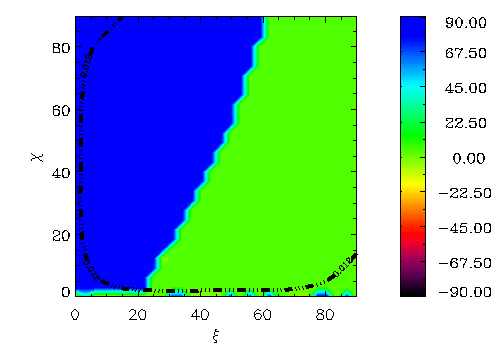
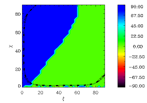
Figure 11: Contour plots of the phase-averaged polarization angles in the ($\chi$, $\xi$) plane for the gaseous atmosphere emission model, with left and right panels corresponding to the optical (B filter) and the X–ray bands respectively.

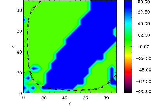
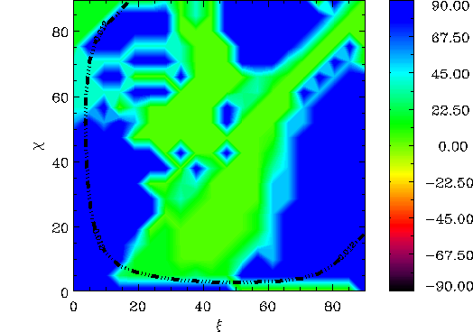
Figure 12: Same as Figure 11 but for the fixed-ion crustal emission model.

For condensed surface emission (in both approximations, fixed and free ions), whereas in the optical band the emitted radiation is dominated by ordinary photons (see Figure 7, left panel), in the X–ray band the two modes have similar intensities, with the emitted radiation being slightly dominated by extraordinary photons for fixed ions (Figure 7, right panel). As a consequence, in the optical band and for viewing angles $\chi>\xi$ we expect that the phase-averaged direction of the photon electric field is parallel to the spin axis, and thus the phase-averaged polarization angle is $\sim 0^{\circ}$. On the contrary, in the X–ray band and again for viewing angles $\chi>\xi$ the phase-averaged direction of the photon electric field is perpendicular to the spin axis, and therefore the expected phase-averaged polarization angle is $\sim 90^{\circ}$. However, the behavior of the polarization angle in the X–rays is quite irregular, due to the fact that the emissivities of the two modes in this band are similar to each other. So, the polarization angle present jumps by 90^∘, which arise because of an even slight predominance of O over X photons or conversely. For the same reason, we do not show the contour plots in the case of free ions, since the corresponding polarization fraction in the two energy bands is even lower than that of the fixed-ions case; hence, the phase-averaged polarization angle behavior for free ions present even more noisy patterns.

The main conclusion is that, by measuring the phase-averaged polarization observables in optical and X–ray bands it is potentially possible to discriminate between atmospheric and crustal emission. The most favorable geometries are those with viewing angles $\chi>\xi$, for which the expected phase-averaged polarization fraction is substantial. If emission is atmospheric, we expect a high phase-averaged polarization fraction in both, optical and X–ray band (although slightly lower in the optical). Whereas, if emission originates from a condensed surface, the phase-averaged polarization fraction should be modest in the optical, with an almost unpolarized signal in the X–ray band.

At the same time, the phase-averaged polarization angle for atmospheric emission is expected to be the same in the optical and X–ray band. On the contrary, for crustal emission the angle measured in the two bands is expected to be different by $\sim 90^{\circ}$ (although this latter consideration is just a theoretical expectation, since realistically the measure of the angle in the X–ray band can not be performed due to low degree of polarization in the signal).

5 Discussion and Conclusions

We studied the polarization properties of the thermal emission from RX J1856 considering different emission models: a NS with a magnetized atmosphere or a condensed surface. The effects of vacuum polarization in the propagation of the radiation in the NS magnetosphere and the rotation of the Stokes parameters were accounted for. Using a ray tracing method and assuming a dipole magnetic field, we derived the polarization observables for different viewing angles $\chi$ and $\xi$. We found that the phase-averaged polarization fraction can be substantially large for viewing angles $\chi>\xi$, which is consistent with previous works (see paper I and references therein). For these viewing angles, in the case of an atmosphere, we found that a) the phase-averaged polarization fraction in the optical band is expected to be lower than in the X–ray band and b) the phase-averaged polarization angle in the optical is the same that in the X–ray band. In the case of condensed surface, we found that a) the phase-averaged polarization fraction in the optical band is substantially higher than in the X–ray band and b) the phase-averaged polarization angle in the optical band is generally shifted by 90^∘ with respect to that in the X–ray band. Therefore, by combining optical and X–ray observations of the polarized emission from RX J1856, it is possible to determine if this XDINS has an atmosphere or a condensed surface.

Our treatment of the surface emission from RX J1856 relied on a number of assumptions/simplifications which are discussed in more detail below. In this respect we stress that our main goal has been to assess to which extent polarization measurements at optical and X–ray energies are effective in discriminating among different emission models, rather than to derive theoretical predictions to be matched with current observations (e.g. through spectral fitting). It is in this spirit that we deliberately chose to restrict to a simple treatment of the emission models we employed, in particular for the atmospheric model.

A major simplification we introduced is that of pure H composition and complete ionization. For the low surface temperature ($\sim 60$ eV) and strong magnetic field ($\sim 10^{13}$ G) of RX J1856, the neutral fraction of H atoms is expected to be $\approx 0.01$–$0.1$ for typical atmospheric densities Potekhin & Chabrier (2004), so that opacities are affected. H atmospheres with partial ionization have been presented e.g. by Potekhin et al. (2004) and Suleimanov et al. (2009, see also ). The major difference with respect to fully ionized models is the appearance of spectral features related to atomic transitions. These features, however, are mainly confined to far UV–soft X–ray range ($\la 0.2$ keV), and fully ionized models give a reasonable description of the spectra at X–ray/optical energies. Moreover, the features are strongly smeared out when the contributions from different surface patches (each with a different $T$ and $\mathbf{B}$) are summed together to obtain the spectrum at infinity (Ho, Potekhin & Chabrier, 2008, see again also Potekhin 2014), similarly to what occurs to the proton cyclotron line Zane et al. (2001).

As noticed by Ho & Lai (2003, see also ), in the atmosphere around a strongly magnetized neutron star vacuum polarization can induce a Mikheyev-Smirnov-Wolfenstein like resonance across which a photon may convert from one mode into the other, with significant changes in the opacities and polarization. While for $B\la 10^{13}$ G this is not going to change the emission spectrum, it still can significantly affect the polarization pattern at least at certain energies. For a photon of energy $E$, the vacuum resonance occurs when the vacuum and plasma contributions to the dielectric tensor become comparable, i.e. where $\rho=\rho_{V}\approx 0.96\times 10^{5}Y_{e}^{-1}(E/1\ \mathrm{keV})^{2}(B/10^{14}\mathrm{G})^{2}f^{-2}$ g cm^-3, where $Y_{\mathrm{e}}=Z/A$ ($Z$ and $A$ are the atomic and mass number of the ions) and $f\sim 1$ is a slowly varying function of $B$. Near the vacuum resonance, the probability of mode conversion is given by $1-P_{\mathrm{jump}}=1-\exp\left[-\pi\left(E/E_{\mathrm{ad}}\right)^{3}/2\right]$, where $E_{\mathrm{ad}}$ depends on the photon energy, on $B$ and on the angle between the photon direction and $\mathbf{B}$ ($\theta_{\mathrm{Bk}}$, van Adelsberg & Lai, 2006, see in particular their eq. 3). For $B\la 10^{13}$ G (as in the case discussed in this work), it is $\rho_{\mathrm{V}}<10^{-3}$ g/cm^-3, i.e. the vacuum resonance is well outside the photospheres of both the ordinary and the extraordinary mode. Moreover, the inequality $E<E_{\mathrm{ad}}$ is satisfied for all photon energies $\la 1$ keV, unless radiation is propagating nearly along the magnetic field direction ($\tan\theta_{\mathrm{Bk}}\la 0.1$). For this reason our assumption of “no mode conversion” at the vacuum resonance, which is equivalent to assume $E\ll E_{\mathrm{ad}}$ (or $P_{\mathrm{jump}}=1$) for all photons, appears reasonable. Further narrow features due to mode collapse and spin-flip transitions are expected very near the broad proton cyclotron resonance (Ho & Lai, 2003; Zane, Turolla & Treves, 2000, see also Melrose & Zhelezniakov 1981 for the case of electrons). In the absence to a complete description of the dielectric tensor in a electrons+ions+vacuum plasma we assumed as a working hypothesis no mode conversion at this frequency.

The present analysis can be extended to other XDINSs as well. The narrow range of surface temperatures inferred from the spectra of XDINSs, $T\sim 50-100$ eV may be important to determine the state of the surface, but it should not have an important effect on the properties of the observable polarization. A significant difference on the polarization properties of XDINSs may be introduced if we consider different magnetic field configurations (see paper I for the example of a twisted magnetic field). However, in general, XDINSs share similar magnetic field configuration, i.e., external dipole magnetic field, and there is no observational evidence for multipolar components or twisted magnetic fields (such as those that may be present in magnetars, see Turolla et al. 2015). This is supported by the good agreement between the magnetic fields derived from timing properties and those inferred from the absorption lines (assuming that they are caused by proton cyclotron resonance, see Turolla 2009), and the absence of non-thermal emission that may be linked to the presence of a twist in the external magnetic field. However, in this respect RX J0720.4-3125 may be an exception. For this XDINS, an absorption feature that is energy-dependent and phase-dependent has been recently reported (Borghese et al., 2015). If this feature is caused by proton cyclotron resonance, then it would be compatible with the presence of a multipolar component confined very close to the NS surface and consistent with a magnetic field $B=10^{14}$ G. The effect of this component on the polarization properties of the radiation has not been assessed, but certainly it can be studied using the method developed in paper I and the emission models here discussed.

References

- Akmal et al. (1998) Akmal A., Pandharipande V. R., & Ravenhall D. G. 1998, Phys. Rev. C, 58, 1804
- Borghese et al. (2015) Borghese A., Rea N., Coti Zelati F., Tiengo A., Turolla R. 2015, ApJ, 807, L20
- Brinkmann (1980) Brinkmann W., 1980, A&A, 82, 352
- Burwitz et al. (2003) Burwitz V., Haberl F., Neuhäuser R., Predehl P., Trümper J., Zavlin V.E. 2003, A&A, 399, 1109
- Fernández & Davis (2011) Fernández R., Davis S. W. 2011, ApJ, 730, 131
- Ginzburg & Ozernoi (1965) Ginzburg V.L., Ozernoi L.M. 1965, Sov. Phys. JETP, 20, 689
- Goriely et al. (2010) Goriely S., Chamel N., & Pearson J. M. 2010, Phys. Rev. C, 82, 035804
- Greenstein & Hartke (1983) Greenstein G., Hartke G.J. 1983, ApJ, 271, 283
- Hambaryan et al. (2011) Hambaryan V., Suleimanov V., Schwope A.D., Neuhäuser R., Werner K., Potekhin A.Y. 2011, A&A, 534, A74
- Harding & Lai (2006) Harding A.K., Lai D. 2006, Rep. Prog. Phys. 69, 2631
- Heyl & Shaviv (2000) Heyl J. S., Shaviv N. J. 2000, MNRAS, 311, 555
- Heyl & Shaviv (2002) Heyl J. S., Shaviv N. J. 2002, Phys. Rev. D, 66, 02300
- Heyl, Shaviv & Lloyd (2003) Heyl J. S., Shaviv N. J., Lloyd D., 2003, MNRAS, 342, 134
- Ho & Lai (2003) Ho W.C.G., Lai D. 2003, MNRAS, 338, 233
- Ho (2007) Ho W. C. G. 2007, MNRAS, 380, 71
- Ho et al. (2007) Ho W.C.G., Kaplan D.L., Chang P., van Adelsberg M., Potekhin A.Y. 2007, MNRAS, 375, 821
- Ho, Potekhin & Chabrier (2008) Ho W.C.G., Potekhin A.Y., Chabrier G. 2008, ApJS, 178, 102
- Jahoda et al. (2015) Jahoda K., Kouveliotou C., Kallman T. R., & Praxys Team 2015, American Astronomical Society Meeting Abstracts, 225, #338.40
- Kaplan & Van Kerkwijk (2009) Kaplan D.L, Van Kerkwijk M.H. 2009, ApJ, 705, 798
- Kaplan et al. (2011) Kaplan D.L., Kamble A., van Kerkwijk M.H., Ho W.C.G. 2011, ApJ, 736, 117
- Lai & Salpeter (1997) Lai D., Salpeter E.E. 1997, ApJ, 491, 270
- Lai (2001) Lai D. 2001, Reviews of Modern Physics, 73, 629
- Lloyd (2003) Lloyd D.A. 2003, arXiv:astro-ph/0303561
- Lloyd, Hernquist & Heyl (2003) Lloyd D.A., Hernquist L., Heyl J.S. 2003, ApJ, 593, 1024
- Medin & Lai (2007) Medin Z., Lai D. 2007, MNRAS, 382, 1833
- Melrose & Zhelezniakov (1981) Melrose D. B., Zhelezniakov V. V. 1981, A&A, 95, 86
- Mignani et al. (2013) Mignani R.P., Vande Putte D., Cropper M., et al. 2013, MNRAS, 429, 3517
- Mori & Ho (2007) Mori K., Ho W.G.C. 2007, MNRAS, 377, 905
- Motch, Zavlin & Haberl (2003) Motch C., Zavlin V., Haberl F. 2003, A&A, 323, 408
- Muslimov & Tsygan (1985) Muslimov A.G., Tsygan A.I. 1986, Sov. Astr., 30, 567
- Page (1995) Page D. 1995, ApJ, 442, 273
- Pavlov & Zavlin (2000) Pavlov G. G., Zavlin V. E. 2000, ApJ, 529, 1011
- Pérez-Azorín et al. (2005) Pérez-Azorín J.F., Miralles J.A., Pons J.A. 2005, A&A, 433, 275
- Pérez-Azorín et al. (2006) Pérez-Azorín J.F., Pons J.A., Miralles J.A., Miniutti G. 2006, A&A, 459, 175
- Pires et al. (2014) Pires A.M., Haberl F., Zavlin V.E., Motch C., Zane S., Hohle M.M. 2014, A&A, 563, A50
- Popov et al. (2003) Popov S.B., Colpi M., Prokhorov M.E., Treves A., Turolla R. 2003, A&A, 406, 111
- Posselt et al. (2008) Posselt B., Popov S.B., Haberl F., Trümper J., Turolla R., Neuhäuser R. 2008, A&A, 482, 617
- Potekhin & Chabrier (2004) Potekhin A.Y., Chabrier G. 2004, ApJ, 600, 317
- Potekhin et al. (2004) Potekhin A.Y., Lai D., Chabrier G., Ho W.C.G. 2004, ApJ, 612, 1034
- Potekhin et al. (2012) Potekhin A.Y., Suleimanov V.F., van Adelsberg M., Werner K. 2012, A&A, 546, A121
- Potekhin (2014) Potekhin A.Y. 2014, Phys. Usp., 57, 735
- Potekhin et al. (2015) Potekhin A. Y., Pons J. A., & Page D. 2015, Space Sci. Rev., 191, 239
- Ruderman (1971) Ruderman M. 1971, Phys. Rev. Lett., 27, 1306
- Sartore et al. (2012) Sartore N., Tiengo A., Mereghetti S., De Luca A., Turolla R., Haberl F. 2012, A&A, 541, A66
- Suleimanov et al. (2009) Suleimanov V., Potekhin A.Y., Werner K. 2009, A&A, 500, 891
- Suleimanov et al. (2010) Suleimanov V., Hambaryan V., Potekhin A.Y., Van Adelsberg M., Neuäuser R., Werner K. 2010, A&A, 522, A111
- Taverna et al. (2015) Taverna R., Turolla R., González Caniulef D., Zane S., Muleri F., Soffitta P. 2015, MNRAS, 454, 3254 (paper I)
- Tiengo & Mereghetti (2007) Tiengo A., Mereghetti S. 2007, ApJ, 657, L101
- Turolla et al. (2004) Turolla R., Zane S.,& Drake J.J. 2004, ApJ, 603, 265
- Turolla (2009) Turolla R. 2009, ASSL, 357, 141
- Turolla et al. (2015) Turolla R., Zane S., & Watts A. L. 2015, Reports on Progress in Physics, 78, 116901
- van Adelsberg et al. (2005) van Adelsberg M., Lai D., Potekhin A.Y., Arras P. 2005, ApJ, 628, 902
- van Adelsberg & Lai (2006) van Adelsberg M., Lai D. 2006, MNRAS, 373, 1495
- van Kerkwijk & Kulkarni (2001) van Kerkwijk M.H., Kulkarni S.R. 2001, A&A, 378, 986
- van Kerkwijk & Kaplan (2008) van Kerkwijk M.H., Kaplan D.L. 2008, ApJ, 673, L163
- Walter et al. (2010) Walter F.M., Eisenbeiß T., Lattimer J.M., Kim B., Hambaryan V., Neuhäuser R. 2010, ApJ, 724, 669
- Weisskopf et al. (2013) Weisskopf M. C., Baldini L., Bellazini R., et al. 2013, Proceedings of the SPIE, 8859, 885908
- Zane, Turolla & Treves (2000) Zane S., Turolla R., Treves A. 2000, ApJ, 537, 387
- Zane et al. (2001) Zane S., Turolla R., Stella A., Treves A. 2001, ApJ, 560, 384
- Zane, Turolla & Drake (2004) Zane S., Turolla R., Drake J.J. 2004, Adv. Sp. Res., 33, 531
- Zane & Turolla (2006) Zane S., Turolla R. 2006, MNRAS, 366, 727