Superconductivity in two-dimensional disordered Dirac semimetals

Abstract

In two-dimensional Dirac semimetals, Cooper pairing instability occurs only when the attractive interaction strength $|u|$ is larger than some critical value $|u_{c}|$ because the density of states vanishes at Dirac points. Disorders enhance the low-energy density of states but meanwhile shorten the lifetime of fermions, which tend to promote and suppress superconductivity, respectively. To determine which of the two competing effects wins, we study the interplay of Cooper pairing interaction and disorder scattering by means of renormalization group method. We consider three types of disorders, including random mass, random gauge potential, and random chemical potential, and show that the first two suppress superconductivity. In particular, the critical BCS coupling $|u_{c}|$ is increased to certain larger value if the system contains only random mass or random gauge potential, which makes the onset of superconductivity more difficult. In the case of random chemical potential, the effective disorder parameter flows to the strong coupling regime, where the perturbation expansion breaks down and cannot provide a clear answer concerning the fate of superconductivity. When different types of disorder coexist in one system, their strength parameters all flow to strong couplings. In the strong coupling regime, the perturbative renormalization group method becomes invalid, and one needs to employ other methods to treat the disorder effects. We perform a simple gap equation analysis of the impact of random chemical potential on superconductivity by using the Abrikosov-Gorkov diagrammatic approach, and also briefly discuss the possible generalization of this approach.

I Introduction

In the Bardeen-Cooper-Schrieffer (BCS) theory of metal superconductors, the Cooper pairing instability caused by a net attractive interaction plays an essential role. A pair of electrons can be bound together by an arbitrarily weak attractive force between them, known as the Cooper theorem. This theorem can by reformulated in the modern renormalization group (RG) theory, which states that the attractive interaction, characterized by a negative coupling constant $u$, is a (marginally) relevant perturbation to the electronic system Shankar1994RMP . The RG equation for $u$ takes the general form

$$\frac{du}{dl}=-cu^{2}$$ (1)

in three-dimensional (3D) metals, where $l$ is a varying length scale and $c$ some constant. This equation tells us that, while a positive $u$ would flow to zero at large $l$, a negative $u$ flows indefinitely to the strong coupling regime no matter how small its initial value is.

In the past three decades, there have been a great deal of research activities devoted to studying the physical properties of electronic systems in which the valence and conduction bands touch at a number of discrete points. Examples include zero-gap semiconductors Fradkin1986 , $d$-wave high-$T_{c}$ cuprate superconductors Orenstein ; Lee2006 , graphene CastroNeto ; Kotov ; DasSarma , topological insulators HasanKane ; ZhangQi ; Vafek , and Weyl semimetals Vafek . These materials exhibit different low-energy behaviors. However, irrespective of the microscopic details, a very common feature shared by these materials is that their low-energy fermionic excitations have a linear dispersion and thus can be described by $N$ species of massless Dirac fermions. Extensive recent theoretic studies Orenstein ; Lee2006 ; Vafek ; CastroNeto ; Kotov ; DasSarma have elaborated that the interparticle interactions can result in non-Fermi-liquid behaviors and certain quantum phase transition. For instance, the long-range Coulomb interaction is able to drive an excitonic insulating transition if its strength is sufficiently large Khveshchenko01 ; Gorbar02 ; Khveshchenko04 ; Liu09 ; LiuNJP11 ; WangNJP12 . The Coulomb interaction can also give rise to unusual spectral behaviors of Dirac fermions CastroNeto ; Kotov . Moreover, the strong spin-orbit coupling may open a finite gap and as such produce a topological insulator Vafek ; HasanKane .

The Cooper pairing of Dirac fermions and the resultant superconducting transition are two subjects of considerable interest Uchoa05 ; Uchoa07 ; Kopnin08 ; Gonzalez08 ; Zhao06 ; Honerkamp08 ; Roy10 ; Roy13 ; Roy14 ; Lee14 ; Yao15 ; Maciejko16 ; Chubukov12 ; Sondhi13 ; Sondhi14 . The superconductivity might be mediated by various bosonic modes, such as phonons or plasmons, in graphene Uchoa07 . When graphene is properly doped such that its Fermi surface is close to a Van Hove singularity Gonzalez08 ; Chubukov12 , even repulsive interaction can result in superconductivity via the Kohn-Luttinger mechanism Kohn65 . Other pairing mechanisms are also possible and have been extensively studied Roy13 . Recent experiment has revealed direct evidence for emergent superconductivity on the surface of a 3D topological insulator Krusin15 .

The Cooper pairing in intrinsic two-dimensional (2D) Dirac semimetals in which the Fermi energy is tuned to precisely the Dirac points is particularly interesting. Previous theoretical and numerical studies Uchoa07 ; Zhao06 ; Honerkamp08 ; Sondhi13 have found that, different from ordinary metals, the Cooper theorem is no longer valid in undoped Dirac semimetals. Because the fermion density of states (DOS) vanishes linearly near the band-touching points, an infinitely weak attraction is not sufficient to bind Dirac fermions together to form Cooper pairs. Cooper pairing can be triggered only when the attraction strength exceeds certain threshold Uchoa07 ; Zhao06 ; Honerkamp08 ; Sondhi13 , i.e., $|u|>|u_{c}|$ with $u_{c}$ being a finite critical value. Hence, there is a quantum phase transition between the semimetallic and superconducting phases, and the critical value $u_{c}$ defines the quantum critical point (QCP). It was proposed recently that a space-time supersymmetry emerges at such a quantum critical point Lee14 ; Maciejko16 , where the massless Dirac fermions and the massless bosonic order parameter are connected by a superconformal algebra.

An interesting question is whether the semimetal-superconductor quantum critical point and the emergent supersymmetry are robust against disorders. To answer this question, it is necessary to investigate the impact of disorders on Cooper pairing. It seems that disorders can promote superconductivity since it may generate a finite zero-energy DOS. However, this could happen only in the presence of disorder that is a relevant perturbation to the system. On the other hand, disorder scattering could break Cooper pairs by shortening the lifetime of Dirac fermions, which would destruct superconductivity. Moreover, there are at least three types of disorder in Dirac semimetals Ludwig1994 ; Nersesyan95 ; Altland02 , including random chemical potential, random mass, and random gauge potential. They have various physical origins, couple to Dirac fermions in different manners, and can result in distinct low-energy behaviors Ludwig1994 ; Nersesyan95 ; Altland02 ; Stauber2005PRB ; Wang2011PRB ; WangLiu2014 . It thus turns out that the effects of disorders are rich and complicated. To acquire a clear understanding of disorder effects, one needs to treat the quartic pairing interaction and fermion-disorder coupling on an equal footing, and analyze how the critical coupling $u_{c}$ is affected by various types of disorder.

Motivated by the above consideration, we will investigate in this paper the disorder effects by performing a perturbative RG analysis within an effective model that contains both quartic pairing interaction and fermion-disorder coupling. Recently, Nandkishore et al. Sondhi13 and Potirniche et al. Sondhi14 have studied the effects of random chemical potential on superconductivity. The main conclusion reached in the mean-field analysis Sondhi13 is that superconductivity is enhanced. In this paper, we will consider the impact of all the three types of disorder.

When the Dirac semimetal contains weak random mass or random gauge potential, the time-reversal symmetry is broken and the Anderson theorem Anderson1959JPCS ; Gorkov08 is certainly invalid. We study the fate of superconductivity by carrying out RG calculations and find that, the critical BCS coupling $|u_{c}|$ increases to certain larger value $|u_{c}^{\prime}|$ when random mass or random gauge potential exists by itself, which makes it more difficult to realize Cooper pairing in realistic materials. The effective strength of these two types of disorder either flows rapidly to zero or remains a small constant at low energies, thus the perturbative RG expansion is under control and the RG results are reliable. We therefore can conclude that superconductivity is more or less suppressed. If $|u|<|u_{c}^{\prime}|$, the Dirac semimetal remains gapless, but its low-energy properties are strongly affected by disorder. Specifically, random mass leads to marginal Fermi liquid (MFL-) like behavior, and random gauge potential induces non-Fermi liquid (NFL) behavior. As $|u_{0}|$ grows upon approaching $|u_{c}^{\prime}|$, the Dirac semimetal enters into a superconducting phase. The nature of such a QCP depends sensitively on the specific type of disorder: for random mass, $|u_{c}^{\prime}|$ defines a QCP between a MFL-like phase and a superconducting state; for random gauge potential, $|u_{c}^{\prime}|$ defines a QCP between a NFL and a superconducting state.

If only random chemical potential exists, the effective strength increases monotonously as the energy is lowered, which means that the perturbative RG method is out of control in the low-energy region and does not give us a clear answer to the fate of superconductivity. Other efficient theoretic tool is needed to study the effects of random chemical potential on superconductivity.

It is widely believed that random chemical potential generates a finite zero-energy DOS, namely $\rho(0)\neq 0$. Similar to Nandkishore et al. Sondhi13 , we assume that the Dirac fermion has only one flavor, with the surface state of a 3D topological insulator being an example. In this case, there is no conventional Anderson localization Ludwig1994 ; Mirlin2006PRB ; Evers08 ; Nomura07 ; Ryu10 , and the fermions become diffusive due to random chemical potential, but remain extended. As this problem cannot be handled by perturbative RG, one might appeal to the mean-field analysis, such as the Abrikosov-Gorkov (AG) approach Gorkov08 ; Sondhi13 . We will present a simple AG analysis and derive the superconducting gap equation after incorporating the impact of random chemical potential. However, it is important to remember that the original AG approach entirely ignores vertex corrections and is justified only in the limit $k_{F}\lambda\gg 1$, where $k_{F}$ is the Fermi momentum and $\lambda$ the mean free path. In 2D Dirac semimetal, we know that $k_{F}\rightarrow 0$, thus the applicability of the AG approach is indeed not well justified. The importance of the vertex corrections needs to be carefully examined, which is an interesting task but goes beyond the scope of the present paper.

After investigating the impact of each single type of disorder, we also consider the coexistence of different types of disorder and find that they have significant mutual influence on each other. Actually, once more than one types of disorder exist in the system, all three types of disorder are present and flow to strong couplings at low energies, driving the system entering into a highly disordered phase. In that case, the fate of superconductivity remains undetermined.

The rest of the paper will be organized as follows. We present the model Hamiltonian in Sec. II and studied the clean limit in Sec. III. We perform the detailed RG calculations in Sec. IV, and then use the RG results to determine the impact of disorder on superconductivity in Sec. V. The mutual influence between different disorders is also studied in this section. We discuss the applicability of the AG approach in Sec. VI. We briefly summarize the results and highlight further works in Sec. VII.

II Effective model

We begin with the following model Hamiltonian Sondhi13 :

$$H=H_{0}+H_{\mathrm{int}}+H_{\mathrm{dis}},$$ (2)

which may describe the Dirac fermions on a 2D honeycomb lattice or on the surface of a three-dimensional topological insulator. The free term of Dirac fermions is

$$H_{0}=\sum_{\mathbf{k}}\Psi^{\dagger}(\mathbf{k})(v_{F}k_{x}\sigma_{1}+v_{F}k_{y}\sigma_{2}-\mu\sigma_{0})\Psi(\mathbf{k}),$$ (3)

where $v_{F}$ is the Fermi velocity and $\mu$ chemical potential. We use $\sigma_{0}$ to denote the $2\times 2$ identity matrix, and $\sigma_{i}$ with $i=1,2,3$ to denote the Pauli matrices, which satisfy the algebra $\left\{\sigma_{i},\sigma_{j}\right\}=2\delta_{ij}$. Since the goal of the present work is to examine the possibility of superconductivity in intrinsic Dirac semimetals, we assume that the Fermi surface is tuned to be exactly at the Dirac points, and henceforth set $\mu=0$. Moreover, we assume there is one flavor of fermion, and neglect the possibility of Anderson localization Ludwig1994 ; Evers08 ; Mirlin2006PRB ; Nomura07 ; Ryu10 .

A possible quartic short-range interaction of Dirac fermions has the following form

$$H_{\mathrm{int}}=\int d^{2}\mathbf{x}\frac{u(\mathbf{x})}{4}\Psi^{\dagger}(\mathbf{x})\sigma_{0}\Psi(\mathbf{x})\Psi^{\dagger}(\mathbf{x})\sigma_{0}\Psi(\mathbf{x}).$$ (4)

For simplicity, the coupling function $u(\mathbf{x})$ can be replaced by a constant $u$, which after renormalization will depend on the varying energy scale. Making a Fourier transformation leads to

$$H_{\mathrm{int}} = \frac{u}{4}\int\frac{d^{2}\mathbf{k}_{1}}{(2\pi)^{2}}\frac{d^{2}\mathbf{k}_{2}}{(2\pi)^{2}}\frac{d^{2}\mathbf{k}_{3}}{(2\pi)^{2}}$$ (5)

$$\times\Psi^{\dagger}_{\mathbf{k}_{1}}\sigma_{0}\Psi_{\mathbf{k}_{2}}\Psi^{\dagger}_{\mathbf{k}_{3}}\sigma_{0}\Psi_{\mathbf{k}_{1}+\mathbf{k}_{3}-\mathbf{k}_{2}},$$

where the spinor $\Psi^{\dagger}_{\mathbf{k}}=\left(c^{\dagger}_{\mathbf{k}\uparrow},c^{\dagger}_{\mathbf{k}\downarrow}\right)$ and $\Psi^{T}_{\mathbf{k}}=\left(c_{\mathbf{k}\uparrow},c_{\mathbf{k}\downarrow}\right)$ are introduced to describe Dirac fermions. Now we can expand the quartic coupling term as

$$\Psi^{\dagger}_{\mathbf{k}_{1}}(\sigma_{0})\Psi_{\mathbf{k}_{2}}\Psi^{\dagger}_{\mathbf{k}_{3}}(\sigma_{0})\Psi_{\mathbf{k}_{4}}$$ (6)

$$= c^{\dagger}_{\mathbf{k}_{1}\uparrow}c_{\mathbf{k}_{2}\uparrow}c^{\dagger}_{\mathbf{k}_{3}\uparrow}c_{\mathbf{k}_{4}\uparrow}+c^{\dagger}_{\mathbf{k}_{1}\uparrow}c_{\mathbf{k}_{2}\uparrow}c^{\dagger}_{\mathbf{k}_{3}\downarrow}c_{\mathbf{k}_{4}\downarrow}$$

$$+c^{\dagger}_{\mathbf{k}_{1}\downarrow}c_{\mathbf{k}_{2}\downarrow}c^{\dagger}_{\mathbf{k}_{3}\uparrow}c_{\mathbf{k}_{4}\uparrow}+c^{\dagger}_{\mathbf{k}_{1}\downarrow}c_{\mathbf{k}_{2}\downarrow}c^{\dagger}_{\mathbf{k}_{3}\downarrow}c_{\mathbf{k}_{4}\downarrow},$$

with $\mathbf{k}_{4}=\mathbf{k}_{1}+\mathbf{k}_{3}-\mathbf{k}_{2}$. The first and fourth terms involve spinors with the same spin if we start from the interaction in Eq. (5), which are indeed not allowed by the Pauli principle Sondhi13 . This implies that the interaction can not capture all the potential four-fermion interactions in a 2D Dirac semimetal. To remedy this, we follow the approach of Ref. Sondhi13 and consider another quartic coupling term

$$H_{\mathrm{int}}\sim\Psi^{\dagger}_{\mathbf{k}}(-i\sigma_{2})\Psi_{\mathbf{k+q}}\Psi^{\dagger}_{\mathbf{p}}(i\sigma_{2})\Psi_{\mathbf{p-q}},$$ (7)

which can be expanded to give

$$\Psi^{\dagger}_{\mathbf{k}_{1}}(-i\sigma_{2})\Psi_{\mathbf{k}_{2}}\Psi^{\dagger}_{\mathbf{k}_{3}}(i\sigma_{2})\Psi_{\mathbf{k}_{4}}$$ (8)

$$= -c^{\dagger}_{\mathbf{k}_{1}\downarrow}c_{\mathbf{k}_{2}\uparrow}c^{\dagger}_{\mathbf{k}_{3}\downarrow}c_{\mathbf{k}_{4}\uparrow}+c^{\dagger}_{\mathbf{k}_{1}\downarrow}c_{\mathbf{k}_{2}\uparrow}c^{\dagger}_{\mathbf{k}_{3}\uparrow}c_{\mathbf{k}_{4}\downarrow}$$

$$+c^{\dagger}_{\mathbf{k}_{1}\uparrow}c_{\mathbf{k}_{2}\downarrow}c^{\dagger}_{\mathbf{k}_{3}\downarrow}c_{\mathbf{k}_{4}\uparrow}-c^{\dagger}_{\mathbf{k}_{1}\uparrow}c_{\mathbf{k}_{2}\downarrow}c^{\dagger}_{\mathbf{k}_{3}\uparrow}c_{\mathbf{k}_{4}\downarrow},$$

which contains all four types of four-fermion coupling term and hence can serve as the starting point.

Figure 1: One-loop correction to fermion propagator. The solid line represents the free fermion propagator.

We then consider the coupling between fermions and disorders, which can be generically described by Ludwig1994 ; Nersesyan95 ; Altland02 ; Stauber2005PRB ; Wang2011PRB ; WangLiu2014

$$H_{\mathrm{dis}}=v_{\Gamma}\int d^{2}\mathbf{x}\Psi^{\dagger}(\mathbf{x})\Gamma\Psi(\mathbf{x})A(\mathbf{x}),$$ (9)

where $v_{\Gamma}$ is a constant and the random field $A(\mathbf{x})$ is taken to be a quenched, Gaussian variable satisfying

$$\langle A(\mathbf{x})\rangle=0,\qquad\langle A(\mathbf{x})A(\mathbf{x}^{\prime})\rangle=\Delta\delta^{2}(\mathbf{x}-\mathbf{x}^{\prime})$$ (10)

with $\Delta$ being a dimensionless variance. The disorders are classified by the definitions of the matrix $\Gamma$. More concretely, $\Gamma=\sigma_{0}$ for random chemical (scalar) potential, and $\Gamma=\sigma_{3}$ for random mass. In the case of random gauge (vector) potential, there are two components for $\Gamma$ and $v_{\Gamma}$: $\Gamma=(\sigma_{1},\sigma_{2})$ and $v_{\Gamma}=(v_{\Gamma 1},v_{\Gamma 2})$. These disorders can be induced by various mechanisms in realistic Dirac fermion materials. For instance, the dominant impurity in $d$-wave cuprate superconductors behaves like a random gauge potential Nersesyan95 , whereas random mass and random chemical potential appear in a 2D orbit antiferromagnet Nersesyan95 . In the context of graphene, random chemical potential might be produced by local defects or neutral absorbed atoms Peres2010RMP ; Mucciolo2010JPCM . The ripple configurations of graphene are usually described by a random gauge potential CastroNeto ; Meyer2007Nature , and the random configurations in the substrates can generate random mass Champel2010PRB ; Kusminskiy2011PRB .

To make our consideration more generic, we suppose all the three types of disorder coexist in the Dirac fermion system and derive the RG equations for all the involved model parameters by employing the replica method to average over the disordered potentials Edwards1975 ; Lerner ; Herbut2008PRL ; Goswami2011PRL ; Roy2014PRB ; Wang2015PLA ; Roy2016PRB ; Roy2016SCP . The impact of each single disorder on the fate of superconductivity can be readily studied by removing the rest two types of disorder. We then consider the interplay of different disorders and examine their mutual influence.

There are three independent parameters in the total Hamiltonian: the fermion velocity $v_{F}$, the quartic coupling constant $u$, and the fermion-disorder coupling $\Delta_{\Gamma}$. They all flow under scaling transformations, and might affect each other since the flow equations are coupled. We will adopt the momentum-shell scheme of RG approach Shankar1994RMP , so it is most convenient to rewrite the effective action in the momentum space

$$S = \int\frac{d\omega d^{2}\mathbf{k}}{(2\pi)^{3}}\Psi^{\dagger}_{\alpha}(i\omega,\mathbf{k})\left[i\omega-v_{F}(k_{x}\sigma_{1}+k_{y}\sigma_{2})\right]\Psi_{\alpha}(i\omega,\mathbf{k})$$ (11)

$$+\frac{u\Lambda^{2}}{4}\int\frac{d\omega d\omega^{\prime}d^{2}\mathbf{k}d\Omega d^{2}\mathbf{q}}{(2\pi)^{7}}\Psi^{\dagger}_{\alpha}(i\omega,\mathbf{k}\uparrow)\sigma_{2}\Psi^{\dagger}_{\alpha}(\omega^{\prime},-\mathbf{k}\downarrow)\Psi_{\alpha}(\Omega,-\mathbf{q}\downarrow)\sigma_{2}\Psi_{\alpha}(i\omega+i\omega^{\prime}-i\Omega,\mathbf{q}\uparrow)$$

$$+\sum_{\Gamma}\frac{\Delta_{\Gamma}}{2}\int\frac{d\omega_{1}d\omega_{2}d^{2}\mathbf{k}_{1}d^{2}\mathbf{k}_{2}d^{2}\mathbf{k}_{3}}{(2\pi)^{8}}\Psi^{\dagger}_{\alpha}(i\omega_{1},\mathbf{k}_{1})\Gamma\Psi_{\alpha}(i\omega_{1},\mathbf{k}_{2})\Psi^{\dagger}_{\beta}(i\omega_{2},\mathbf{k}_{3})\Gamma\Psi_{\beta}(i\omega_{2},\mathbf{k}_{1}+\mathbf{k}_{2}+\mathbf{k}_{3}).$$

This action has been obtained by applying the replica trick to average over random potential $A(\mathbf{r})$, with $\alpha$ and $\beta$ being two replica indices and $\Delta_{\Gamma}=\Delta v_{\Gamma}^{2}$. To distinguish different random potentials, we introduce three new parameters $\Delta_{M}$, $\Delta_{S}$, and $\Delta_{V}$ to characterize the effective strength of the four-fermion couplings generated after averaging over random mass, random chemical potential, and random gauge potential, respectively. Notice that the coupling $u$ multiples a factor $\Lambda^{2}$, whose meaning will be explained in Sec. IV.

The first term is the free fixed point of the action, and should be kept invariant under the following re-scaling transformations

$$k_{i} = k^{\prime}_{i}e^{-l},$$ (12)

$$\omega = \omega^{\prime}e^{-l},$$ (13)

$$\Psi_{\alpha}(i\omega,\mathbf{k}) = \Psi_{\alpha}^{\prime}(i\omega^{\prime},\mathbf{k}^{\prime})e^{2l},$$ (14)

where $l$ is a freely varying length scale. We will examine how the other two interaction terms are modified under these transformations in the next two sections.

III Cooper pairing in the clean limit

We first consider the case of clean Dirac semimetals. The existence of a critical strength of attractive interaction, namely $u_{c}$, is well-known, and has been obtained previously by various methods Uchoa07 ; CastroNeto ; Sondhi13 . For completeness sake, we present the RG derivation of $u_{c}$ in this section and foresee the possible impact of disorders.

The leading correction to the fermion self-energy due to quartic interaction is shown in Fig. 1. Using the free fermion propagator

$$G_{0}(i\omega,\mathbf{k})=\frac{1}{i\omega-v_{F}(k_{x}\sigma_{1}+k_{y}\sigma_{2})},$$ (15)

it is easy to check that the self-energy is

$$\Sigma_{f}\sim\mathrm{Tr}\int^{\infty}_{-\infty}\frac{d\omega}{(2\pi)}\int_{b}^{1}\frac{d^{2}\mathbf{k}}{(2\pi)^{2}}(-i\sigma_{2})G_{0}(k)=0.$$ (16)

This result simply implies that the quartic interaction does not lead to renormalization of fermion velocity $v_{F}$, so we only need to consider the renormalization of the coupling constant $u$.

We now proceed to compute the one-loop corrections to the quartic coupling term. There are three sorts of diagrams for this vertex corrections, as shown in Fig. 2. Borrowing the terminology of Shankar Shankar1994RMP , these three diagrams are dubbed ZS, ZS’, and BCS diagrams, respectively. We find it convenient to first consider BCS diagram, which yields

$$u^{\mathrm{BCS}}_{\mathrm{1L}} = 4\left(\frac{u\Lambda^{2}}{4}\right)^{2}\mathrm{Tr}\int^{\infty}_{-\infty}\frac{d\omega^{\prime}}{(2\pi)}\int_{b}^{1}\frac{d^{2}\mathbf{k^{\prime}}}{(2\pi)^{2}}$$ (17)

$$\times\sigma_{2}G_{0}(k^{\prime})\sigma_{2}G_{0}(\mathbf{P}-k^{\prime})$$

$$= \left(\frac{1}{b^{-2}}\frac{u\Lambda^{2}}{4}\right)\left(\frac{u\Lambda^{2}}{4}\right)\frac{l}{\pi v_{F}},$$

with momentum $\mathbf{P}=0$ in the Cooper channel Sondhi13 . We then move to compute the contributions of the ZS and ZS’ diagrams Shankar1994RMP . It is straightforward to obtain

$$u^{\mathrm{ZS}}_{\mathrm{1L}} = -\frac{u^{2}_{0}}{2}\mathrm{Tr}\int^{\infty}_{-\infty}\frac{d\omega^{\prime}}{(2\pi)}\int_{b}^{1}\frac{d^{2}\mathbf{k^{\prime}}}{(2\pi)^{2}}$$ (18)

$$\times(\sigma_{2})G_{0}(k^{\prime})(\sigma_{2})G_{0}(k^{\prime}+\mathbf{Q}),$$

$$u^{\mathrm{ZS^{\prime}}}_{\mathrm{1L}} = \frac{u^{2}_{0}}{2}\mathrm{Tr}\int^{\infty}_{-\infty}\frac{d\omega^{\prime}}{(2\pi)}\int_{b}^{1}\frac{d^{2}\mathbf{k^{\prime}}}{(2\pi)^{2}}$$ (19)

$$\times(\sigma_{2})G_{0}(k^{\prime})(\sigma_{2})G_{0}(k^{\prime}+\mathbf{Q^{\prime}}),$$

where $\mathbf{Q}=\mathbf{k}_{2}-\mathbf{k}_{1}$ and $\mathbf{Q^{\prime}}=\mathbf{k}_{4}-\mathbf{k}_{1}$, also defined in Fig. 2. In ordinary metals which possess a finite Fermi surface, the transferred momenta $Q$ and $Q^{\prime}$ are suppressed due to the large Fermi momentum, thus the ZS and ZS’ contributions are negligible compared to the BCS contribution Shankar1994RMP . In a Dirac fermion system, the Fermi momentum $k_{F}\rightarrow 0$, and one needs to be more careful when dealing with the ZS and ZS’ diagrams. Since $\mathbf{k}_{2}$ and $\mathbf{k}_{1}$ are both external momenta, they are much smaller than the shell momenta to be integrated out in the process of carrying out RG calculations Shankar1994RMP . Accordingly, the difference $\mathbf{Q}=\mathbf{k}_{2}-\mathbf{k}_{1}$ can be approximated as $\mathbf{Q}=0$. Under these approximations, we compute ZS diagram and get

$$u^{\mathrm{ZS}}_{\mathrm{1L}}=2u^{\mathrm{BCS}}_{\mathrm{1L}}.$$ (20)

As for ZS’ diagram, we assume a finite $Q^{\prime}$ but henceforth utilize $Q$ to substitute $Q^{\prime}$ for notational simplicity. After introducing a variable $\delta\equiv 2Q-Q^{2}$ with $Q\in(0,\sqrt{2}b)$ and carrying straightforward calculations, we obtain

$$u^{\mathrm{ZS^{\prime}}}_{\mathrm{1L}} \equiv -2u^{\mathrm{BCS}}_{\mathrm{1L}}f_{Q},$$ (21)

where

$$f_{Q} \equiv \frac{2-2(1-\delta)^{\frac{3}{2}}}{3\delta}+\frac{4(Q^{2}_{x}-Q^{2}_{y})}{15\delta^{3}}$$ (22)

$$\times\left[4-5\delta+\sqrt{1-\delta}\left(\delta^{2}+3\delta-4\right)\right].$$

Summing over the contributions from BCS, ZS, and ZS’ diagrams yields

$$u_{\mathrm{1L}} = u^{\mathrm{BCS}}_{\mathrm{1L}}+u^{\mathrm{ZS}}_{\mathrm{1L}}+u^{\mathrm{ZS^{\prime}}}_{\mathrm{1L}}$$ (23)

$$= \left[1+2\left(1-f_{Q}\right)\right]u^{\mathrm{BCS}}_{\mathrm{1L}}.$$

Since the system preserves translational symmetry, one can show that

$$u_{\mathrm{1L}}=\left[1+2\left(1-f^{\prime}_{Q}\right)\right]u^{\mathrm{BCS}}_{\mathrm{1L}},$$ (24)

where

$$u^{\mathrm{BCS}}_{\mathrm{1L}} = \frac{u^{2}_{0}}{16\pi v_{F}}l,$$ (25)

$$f^{\prime}_{Q} \equiv \frac{2-2(1-\delta)^{\frac{3}{2}}}{3\delta}.$$ (26)

Since the transferred momentum $Q$ is very small, it is easy to verify that

$$\lim_{Q\rightarrow 0}f^{\prime}_{Q}=\lim_{\delta\rightarrow 0}f^{\prime}_{Q}=1,$$ (27)

which immediately indicates that

$$\lim_{Q\rightarrow 0}u_{\mathrm{1L}}=u^{\mathrm{BCS}}_{\mathrm{1L}}.$$ (28)

Figure 2: One-loop vertex corrections to the pairing interaction term, known as ZS, ZS’, and BCS diagrams respectively. The fourth momentum is determined according to momentum conservation, namely $\mathbf{k}_{4}=\mathbf{k}_{1}+\mathbf{k}_{3}-\mathbf{k}_{2}$.

From the above calculations, we infer that the ZS and ZS’ contributions cancel each other provided that the external momenta are sufficiently small. Since our focus is on the low-energy asymptotic behaviors of the system, we will neglect the ZS and ZS’ diagrams in the next two sections and retain only the BCS diagram. For completeness, we will revisit the effects of ZS and ZS’ diagrams in Sec. V.5, where it will be showed that including their contributions does not alter our basic conclusion.

Discarding the ZS and ZS’ diagrams and adding the vertex correction induced by the BCS diagram to the bare $u$ term, we find that the BCS coupling flows according to the following equation:

$$\frac{du}{dl}=-\left(1+\frac{u}{8\pi v_{F}}\right)u,$$ (29)

The critical coupling can be easily obtained from this equation:

$$u_{c}=-8\pi v_{F}.$$ (30)

The corresponding flow diagram is presented in Fig. 3. If the bare value $|u_{0}|<|u_{c}|$, the pairing interaction flows to the trivial fixed point and Cooper pairing cannot be formed. On the contrary, if $|u_{0}|>|u_{c}|$, the attractive interaction flows to the strong coupling regime, which leads to Cooper pairing instability.

The above results are not new and have already been obtained previously by various approaches Uchoa07 ; Zhao06 ; Honerkamp08 ; Sondhi13 . In the next section, we will include three types of disorder and study their interplay with the pairing interaction by carrying out detailed RG calculations. In that case, the flow equation of $u$ might be substantially influenced by disorders, and, as a consequence, superconductivity might be enhanced or suppressed.

IV RG calculations in disordered Dirac semimetals

In this section, we study the interplay of Cooper pairing and disorder by performing detailed RG analysis. The aforementioned three types of disorders are supposed to coexist in the system. The impact of each disorder can be separately examined by removing the rest two.

Following Nandkishore et al. Sondhi13 , we wish to start our analysis directly from an effective BCS-type interaction term that includes only the pairing between two Dirac fermions with opposite momenta and spin (in case of singlet pairing). To this end, we need to project the interaction term (7) onto the Cooper channel Sondhi13 , which is justified because the ZS and ZS’ diagrams cancel each other at low energies. This can be formally achieved by introducing a delta function $\delta^{2}(\mathbf{p}+\mathbf{k})$ to $H_{\mathrm{int}}$ and then integrate over $\mathbf{p}$. However, since a delta function $\delta^{2}(\mathbf{p})$ scales like $\mathbf{p}^{-2}$, it might alter the dimension of the coupling constant $u$. To solve this problem, here we introduce an UV cutoff $\Lambda$ and write the effective BCS interaction as

$$H_{\mathrm{BCS}}=\frac{u\Lambda^{2}}{4}\sum_{\mathbf{k},\mathbf{q}}\Psi^{\dagger}_{\mathbf{k},\uparrow}(-i\sigma_{2})\Psi^{\dagger}_{-\mathbf{k},\downarrow}\Psi_{-\mathbf{q},\downarrow}(i\sigma_{2})\Psi_{\mathbf{q},\uparrow}.$$ (31)

Here, $\Lambda$ can be considered as the contributions from the neglected non-BCS coupling terms. It should scale as $\mathbf{p}^{2}$ and becomes progressively unimportant as one goes to lower and lower energies. An alternative approach is to regard Eq. (31) as the starting point and define a new effective coupling constant $u_{\mathrm{eff}}=u\Lambda^{2}/4$, which will lead us to the same results.

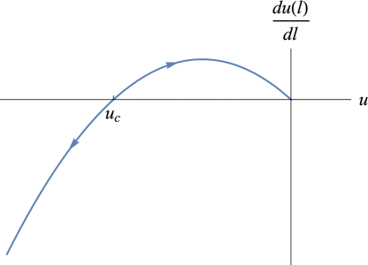
Figure 3: Critical value $u_{c}$ is an unstable infrared fixed point. Upon leaving this point, the BCS pairing coupling either flows to zero, or grows monotonously, leading to Cooper pairing instability.

It is necessary to pause here and briefly remark on the validity of introducing the above attractive interaction term. To acquire a net attraction between Dirac fermions, the attractive force mediated by either phonons or plasmons should be larger than the Coulombic repulsive force Uchoa07 . Due to the vanishing of zero-energy DOS, the Coulomb interaction is only poorly screened by the particle-hole continuum CastroNeto ; Kotov and thus makes it hard to achieve a net attraction. However, the strength of Coulomb interaction can be substantially reduced when the Dirac semimetal is placed on some metallic substrate CastroNeto ; Kotov ; DasSarma . Moreover, disorders may generate a finite DOS at the Dirac points, which also strongly suppresses the Coulomb interaction via static screening Liu09 ; LiuNJP11 . Therefore, it is in principle possible for Dirac semimetals to develop a net attractive interaction. Our following analysis will be based on the assumption that a net attraction is realized in an intrinsic 2D Dirac semimetal.

Figure 4: One-loop correction to fermion propagator due to disorder scattering. Here, the dashed line represents the disorder scattering and $\Gamma_{a}$ should sum over all the three types of disorder.

Figure 5: One-loop corrections to the disorder strength in the replica limit. The repeated $\Gamma_{a,b}$ should sum over all the three types of disorder.

Figure 6: One-loop vertex corrections to the pairing interaction due to disorder scattering.

In the presence of disorders, the Dirac fermions receive additional self-energy corrections due to disorder scattering. The leading correction presented in Fig. 4 leads to

$$\Sigma_{\mathrm{dis}}(i\omega) = \sum_{\Gamma}\Delta_{\Gamma}\int\frac{d^{2}\mathbf{q}}{(2\pi)^{2}}\Gamma G_{0}(i\omega,\mathbf{q})\Gamma$$ (32)

$$= -i\omega\frac{\Delta_{M}+\Delta_{S}+2\Delta_{V}}{2\pi v^{2}_{F}}l.$$

To study the renormalization of disorder parameter $\Delta_{\Gamma}$, we next would consider the vertex corrections to the effective quartic coupling induced by disorder averaging procedure, as schematically shown in Fig. 5. Clearly, Fig. 5(a) represents the bare vertex, and we only need to compute the rest four diagrams given by Fig. 5(b-e). The contribution of Fig. 5(b) is given by

$$\delta\Delta_{\Gamma}^{b} = \Delta_{\Gamma}\sum_{\Gamma_{b}}\Delta_{b}\int\frac{d^{2}\mathbf{q}}{(2\pi)^{2}}\Gamma_{b}G_{0}(\mathbf{q})\Gamma G_{0}(\mathbf{q})\Gamma_{b}.$$ (33)

The matrix $\Gamma$ has different expression in the case of different types of disorder. For random chemical potential, $\Gamma=\sigma_{0}$ and we have

$$\delta\Delta_{S}^{b}=\frac{(\Delta_{S}+\Delta_{M}+2\Delta_{V})\Delta_{S}}{2\pi v_{F}^{2}}\sigma_{0}l.$$ (34)

For random mass, $\Gamma=\sigma_{3}$ and we have

$$\delta\Delta_{M}^{b} = \frac{-(\Delta_{S}+\Delta_{M}-2\Delta_{V})\Delta_{M}}{2\pi v_{F}^{2}}\sigma_{3}l.$$ (35)

For random gauge potential, there are two components, namely $\Gamma=\sigma_{1}$ and $\Gamma=\sigma_{2}$. In both of these two cases, we find that

$$\delta\Delta_{V}^{b}=0.$$ (36)

The contributions form Fig. 5(c) and Fig. 5(d) are best computed at once. It is convenient to sum them up and obtain

$$\delta\Delta_{\Gamma}^{c+d} = \sum_{\Delta_{a}}\sum_{\Delta_{b}}\Delta_{a}\Delta_{b}\int\frac{d^{2}\mathbf{p}}{(2\pi)^{2}}\psi^{\dagger}_{\alpha}[\Gamma_{a}G_{0}(0,\mathbf{p})\Gamma_{b}]\psi_{\alpha}$$ (37)

$$\times\psi^{\dagger}_{\beta}[\Gamma_{b}G_{0}(0,\mathbf{p})\Gamma_{a}+\Gamma_{a}G_{0}(0,-\mathbf{p})\Gamma_{b}]\psi_{\beta}.$$

Straightforward calculations yield

$$\delta\Delta_{S}^{c+d} = \frac{2\Delta_{M}\Delta_{V}}{2\pi v_{F}^{2}}l(\bar{\psi}_{\alpha}\sigma_{0}\psi_{\alpha})(\bar{\psi}_{\beta}\sigma_{0}\psi_{\beta}),$$ (38)

$$\delta\Delta_{M}^{c+d} = \frac{2\Delta_{S}\Delta_{V}}{2\pi v_{F}^{2}}l(\bar{\psi}_{\alpha}\sigma_{3}\psi_{\alpha})(\bar{\psi}_{\beta}\sigma_{3}\psi_{\beta}),$$ (39)

$$\delta\Delta_{V}^{c+d} = \frac{\Delta_{M}\Delta_{S}}{2\pi v_{F}^{2}}l(\bar{\psi}_{\alpha}\sigma_{j}\psi_{\alpha})(\bar{\psi}_{\beta}\sigma_{j}\psi_{\beta}),$$ (40)

which apply to the case of random chemical potential, random mass, and random gauge potential, respectively. Here, the repeated index $j$ sums over the two components of random gauge potential. For all the other cases with $\Gamma_{a}=\Gamma_{b}=\sigma_{0,1,2,3}$, these two diagrams cancel each other and make no contributions to the vertex.

There is now only one diagram left, given by Fig. 5(e). Similar to the one-loop correction to the coupling $u$, there are three possibilities, corresponding to ZS, ZS’, and BCS like diagrams, as explicitly shown in Ref. Sondhi13 . As we have illustrated in Sec. III, the ZS and ZS’ diagrams cancel each other and the BCS diagram makes no contribution because the loop momentum lies in the slim shell due to the momentum restriction, as showed by Fig.1. Finally, as argued in Ref. Sondhi13 , this sort of diagram simply vanishes and contributes nothing to the quartic coupling term represented by parameter $\Delta_{\Gamma}$.

Apart from the fermion-disorder vertex corrections, there are two one-loop diagrams contributing to the BCS interaction $u$ due to disorders, as given by Fig. 6. It is easy to find that

$$u^{\mathrm{1L}}_{\mathrm{dis1}} = \frac{u}{4}\left(\frac{\Delta_{M}+\Delta_{S}+2\Delta_{V}}{4\pi v_{F}}\right),$$ (41)

$$u^{\mathrm{1L}}_{\mathrm{dis2}} = -\frac{u}{4}\left(\frac{\Delta_{M}+\Delta_{S}+2\Delta_{V}}{4\pi v_{F}}\right).$$ (42)

Apparently, these two contributions cancel precisely, and thus can be simply dropped.

Now we have evaluated all the leading corrections to fermion self-energy and disorder vertex, and are ready to derive the RG equations. To proceed, we need to integrate out the modes defined in the momentum shell $b\Lambda<k<\Lambda$, where $b$ can be written as $b=e^{-l}$. Under the scaling transformation $k_{i}=k^{\prime}_{i}e^{-l}$ and $\omega=\omega^{\prime}e^{-l}$, the fermion field and disorder potential should transform as follows Huh2008

$$\Psi_{\alpha}(i\omega,\mathbf{k}) = \Psi_{\alpha}^{\prime}(i\omega^{\prime},\mathbf{k}^{\prime})e^{\frac{1}{2}\int_{0}^{l}dl(4-\eta)}.$$ (43)

where $\eta$ is an anomalous dimension for the fermion field $\Psi$ induced by disorders.

To compute $\eta$, we first redefine the effective parameter for random potential as follows

$$\frac{\Delta_{\Gamma}}{2\pi v_{F}^{2}}\rightarrow\Delta_{\Gamma}.$$ (44)

Adding the fermion self-energy $\Sigma_{\mathrm{dis}}(i\omega)=-i\omega(\Delta_{M}+\Delta_{S}+2\Delta_{V})l$ to the free fermion action, we have

$$\int^{b}_{0}\frac{d\omega}{2\pi}\frac{d^{2}\mathbf{k}}{(2\pi)^{2}}\Psi^{\dagger}_{\alpha}[1+(\Delta_{M}+\Delta_{S}+2\Delta_{V})l](i\omega)\Psi_{\alpha}$$ (45)

$$= \int^{b}_{0}\frac{d\omega}{2\pi}\frac{d^{2}\mathbf{k}}{(2\pi)^{2}}\Psi^{\dagger}_{\alpha}(i\omega)e^{(\Delta_{M}+\Delta_{S}+2\Delta_{V})l}\Psi_{\alpha},$$

which after rescaling transformations becomes

$$\int^{1}_{0}\frac{d\omega}{2\pi}\frac{d^{2}\mathbf{k}}{(2\pi)^{2}}\Psi^{\dagger}_{\alpha}(i\omega)e^{-\eta l+(\Delta_{M}+\Delta_{S}+2\Delta_{V})l}\Psi_{\alpha}.$$ (46)

This term is required to return to its original form, which forces us to demand that

$$\eta=\Delta_{M}+\Delta_{S}+2\Delta_{V}.$$ (47)

By using the above anomalous dimension and the one-loop quantum corrections we have just computed, we eventually obtain the following RG equations:

$$\frac{dv_{F}}{dl} = \!\!-(\Delta_{M}+\Delta_{S}+2\Delta_{V})v_{F},$$ (48)

$$\frac{d\Delta_{S}}{dl} = \!\!2(\Delta_{S}+2\Delta_{V}+\Delta_{M})\Delta_{S}+4\Delta_{M}\Delta_{V},$$ (49)

$$\frac{d\Delta_{M}}{dl} = \!\!-2(\Delta_{M}-2\Delta_{V}+\Delta_{S})\Delta_{M}+4\Delta_{S}\Delta_{V},$$ (50)

$$\frac{d\Delta_{V}}{dl} = \!\!2\Delta_{S}\Delta_{M},$$ (51)

$$\frac{du}{dl} = \!\!-\left[1+2(\Delta_{M}+\Delta_{S}+2\Delta_{V})+\frac{u}{8\pi v_{F}}\right]\!\!u.$$ (52)

We notice that Eqs. (49)-(51) are in accordance with the results obtained previously in Refs. Aleiner2006PRL ; Aleiner2008PRB ; Foster12 . In the next section, we will use these RG equations to analyze how disorders affect the formation of superconductivity.

V RG analysis of the disorder effects on superconductivity

In this section, we will first consider the impact of each single disorder on superconductivity by simply removing the rest two types of disorder from the complete set of RG equations. We pay special attention to the (ir)relevance of the effective disorder parameter $\Delta_{\Gamma}$ and how the BCS coupling $u$ is modified by the disorder. In addition, we are also interested in the low-energy behaviors of some physical quantities, including the fermion velocity $v_{F}$, quasi-particle residue $Z_{f}$, and fermion DOS $\rho(\omega)$.

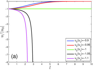
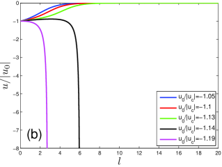
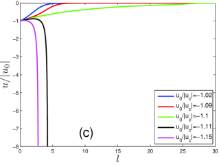
Figure 7: (Color online) Flow of pairing interaction parameter $u$ in the case of: (a) clean limit; (b) random mass with $\Delta_{M}^{0}=0.1$; (c) random gauge potential with $\Delta_{V}^{0}=0.05$. The parameter $u$ with a small initial value flows to zero at large $l$, whereas a sufficiently large $u$ flows rapidly to strong coupling, signalling the onset of superconductivity. A critical value for $u$ exists in each case, but the absolute value $|u_{c}^{\prime}|$ obtained in the presence of disorder is always larger than $|u_{c}|$ obtained in clean limit. It can be verified that stronger disorder gives rise to larger value of $|u_{c}^{\prime}|$, which further suppresses superconductivity.

V.1 Random mass

In the case that random mass exists alone in the system, we can simply set $\Delta_{S}=\Delta_{V}=0$. Now, the complete set of RG equations are simplified to

$$\frac{dv_{F}}{dl} = -\Delta_{M}v_{F},$$ (53)

$$\frac{d\Delta_{M}}{dl} = -2\Delta_{M}^{2},$$ (54)

$$\frac{du}{dl} = -\left[1+2\Delta_{M}+\frac{u}{8\pi v_{F}}\right]u.$$ (55)

It is clear that the velocity $v_{F}$ and disorder parameter $\Delta_{M}$ are no longer constants, but flow with varying length scale $l$ according to Eq. (53) and Eq. (54). To determine the new critical value $|u_{c}^{\prime}|$, we need to solve these two RG equations. It is easy to find that Eq. (54) has a solution

$$\Delta_{M}(l)=\frac{\Delta_{M}^{0}}{1+2\Delta_{M}^{0}l}.$$ (56)

Substituting Eq. (56) to Eq. (53) and solving the differential equation gives rise to

$$v_{F}(l)=\frac{v_{F}^{0}}{\sqrt{2\Delta_{M}^{0}l+1}}.$$ (57)

Apparently, $\Delta_{M}$ and $v_{F}$ decrease very slowly with growing $l$ and eventually vanish as $l\rightarrow+\infty$. After including random mass, the flow of $u$ for different values of $u_{0}/|u_{c}|$ at $\Delta_{M}^{0}=0.1$ is shown in Fig. 7(b). In the clean limit, for the specific initial values of $u_{0}/|u_{c}|=-1.05$, $u_{0}/|u_{c}|=-1.1$, and $u_{0}/|u_{c}|=-1.13$, $u$ flows rapidly to the strong coupling regime, which signals the onset of superconductivity. However, after random mass is included, $u$ flows to zero in the lowest-energy limit starting from the same initial values, which implies that the system remains gapless. It is therefore clear that random mass tends to suppress superconductivity. For larger initial values of $u_{0}/|u_{c}|$, $u$ still flows to strong coupling. The new QCP is located at $u_{c}^{\prime}$, which is greater than $u_{c}$.

The above RG analysis show that the effective disorder parameter $\Delta_{M}$ vanishes ultimately as $l\rightarrow+\infty$. However, $\Delta_{M}$ flows to zero slowly with growing $l$. Concretely, according to Eq. (56), we find that $\Delta_{M}\sim\frac{1}{l}$. In the spirit of RG theory, this means that random mass is marginally irrelevant in a 2D Dirac fermion system. Nevertheless, before $\Delta_{M}$ flowing to zero, random mass can still induce weak corrections to observable quantities of the system. As shown in the above analysis, random mass drives $v_{F}$ to vanish at very low energies and increases the critical BCS coupling $u_{c}$.

We now analyze three important quantities, namely the Landau damping rate, the quasiparticle residue $Z_{f}$, and the low-energy DOS. The residue is usually defined as

$$Z_{f}=\frac{1}{1-\frac{\partial\mathrm{Re}\Sigma^{R}(\omega)}{\partial\omega}},$$ (58)

where $\mathrm{Re}\Sigma^{R}$ is the real part of retarded fermion self-energy. By virtue of the RG results and also according to the one-loop self-energy given by Eq. (32), it is convenient to express the residue in the following form WangLiu2014 ; WangLiuZhang16

$$\frac{dZ_{f}}{dl}=-\Delta_{M}Z_{f}.$$ (59)

Making use of Eq. (56), it is easy to find that $Z_{f}\sim\frac{1}{\sqrt{2\Delta_{M}^{0}l+1}}\rightarrow 0$ in the limit $l\rightarrow+\infty$. Hence, the Dirac fermions are not well-defined Landau quasiparticles. Using the scaling relation $\omega=\omega_{0}e^{-l}$, where $\omega_{0}$ is a UV cutoff, we get

$$\mathrm{Re}\Sigma^{R}(\omega)\sim\omega\left[\ln\left(\frac{\omega_{0}}{\omega}\right)\right]^{\frac{1}{2}}.$$ (60)

According to the Kramers-Kronig (KK) relation, the imaginary part of retarded self-energy depends on $\omega$ as

$$\mathrm{Im}\Sigma^{R}(\omega)\sim\frac{\omega}{\left[\ln\left(\frac{\omega_{0}}{\omega}\right)\right]^{\frac{1}{2}}},$$ (61)

which apparently is a MFL-like behavior. The RG equation for the low-energy DOS is give by WangLiu2014 ; WangLiuZhang16

$$\frac{d\ln\rho(\omega)}{d\ln(\omega)}=\frac{1-\Delta_{M}}{1+\Delta_{M}}.$$ (62)

After solving this equation, we obtain

$$\rho(\omega)\sim\omega\ln\left(\frac{\omega_{0}}{\omega}\right).$$ (63)

Comparing to the low-energy DOS $\rho(\omega)\sim\omega$ for clean, non-interacting 2D Dirac semimetal, we find that the low-energy DOS $\rho(\omega)$ is enhanced by random mass.

Based on the above analysis, we plot the schematic phase diagram spanned by $\Delta_{M}^{0}$ and $u_{0}$ in Fig. 8(a). In the clean limit, the critical coupling $u_{c}$ defines a QCP between a non-interacting Dirac semimetallic phase and a superconducting phase. In contrast, in the presence of random mass, the new critical coupling $u_{c}^{\prime}$, whose absolute value is larger than $|u_{c}|$, corresponds to a QCP between a MFL-like phase and a superconducting phase.

V.2 Random gauge potential

Setting $\Delta_{S}=\Delta_{M}=0$, the RG equations become

$$\frac{dv_{F}}{dl} = -2\Delta_{V}v_{F},$$ (64)

$$\frac{d\Delta_{V}}{dl} = 0,$$ (65)

$$\frac{du}{dl} = -\left[1+4\Delta_{V}+\frac{u}{8\pi v_{F}}\right]u.$$ (66)

We know from Eq. (65) that random gauge potential is marginal and $\Delta_{V}$ should be a constant, namely

$$\Delta_{V}(l)=\Delta_{V}^{0}.$$ (67)

Substitute this constant to Eq. (64), we get

$$v_{F}(l)=v_{F}^{0}e^{-2\Delta_{V}^{0}l}.$$ (68)

Random gauge potential drives the fermion velocity to decay exponentially, which in turn alters the critical coupling $u_{c}$. At the chosen value $\Delta_{V}^{0}=0.1$, the flow of $u$ at different initial values of $u_{0}/|u_{c}|$ is depicted in Fig. 7(c). We observe that random gauge potential modifies the critical value $u_{c}$ to $u_{c}^{\prime}$ with a larger absolute value, and thus suppresses superconductivity. Based on Eqs. (58) and (67), we find that the residue behaves as

$$Z_{f}(l)=e^{-2\Delta_{V}^{0}l},$$ (69)

which vanishes rapidly with growing $l$. It is easy to obtain

$$\mathrm{Im}\Sigma^{R}(\omega)\sim\omega^{1-2\Delta_{V}^{0}}.$$ (70)

This is typical NFL behavior since $\Delta_{V}^{0}>0$. Using Eqs. (62) and (67), we get the low-energy DOS

$$\rho(\omega)=\omega^{\frac{1-2\Delta_{V}^{0}}{1+2\Delta_{V}^{0}}},$$ (71)

which is enhanced by random gauge potential.

If we fix $\Delta_{V}^{0}$ and tune the coupling $u$, the system undergoes a quantum phase transition between a NFL and a superconducting phase, with $u_{c}^{\prime}$ being the QCP. The schematic phase diagram in the space spanned by $\Delta_{V}^{0}$ and $u_{0}$ is shown in Fig. 8(b). There is a critical line on the phase diagram, separating the superconducting phase from the NFL phase.

V.3 Random chemical potential

In the case of random chemical potential, the RG equations are

$$\frac{dv_{F}}{dl} = -\Delta_{S}v_{F},$$ (72)

$$\frac{d\Delta_{S}}{dl} = 2\Delta_{S}^{2},$$ (73)

$$\frac{du}{dl} = -\left[1+2\Delta_{S}+\frac{u}{8\pi v_{F}}\right]u.$$ (74)

Similarly, solving Eq. (73) gives

$$\Delta_{S}(l)=\frac{\Delta_{S}^{0}}{1-2\Delta_{S}^{0}l}.$$ (75)

Substituting Eq. (75) to Eq. (72), and solving the differential equation we get

$$v_{F}(l)=v_{F}^{0}\sqrt{1-2\Delta_{S}^{0}l}.$$ (76)

There exists a characteristic length scale $l_{c}=1/2\Delta_{s}^{0}$. As $l$ approaches $l_{c}$ from below, the effective strength parameter $\Delta_{S}\rightarrow\infty$ and the fermion velocity $v_{F}\rightarrow 0$. It is thus clear that random chemical potential is a relevant perturbation to the system. This behavior is usually interpreted as a signature that the Dirac fermion system enters into a disorder-controlled diffusive state Altland02 . However, since $\Delta_{S}$ flows to the strong coupling, the perturbative RG method progressively breaks down and cannot provide a clear answer to the fate of superconductivity.

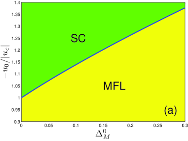
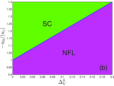
Figure 8: (Color online) Phase diagram in the space spanned by $\Delta_{\Gamma}$ and $u_{0}$ in the case of (a) random mass; (b) random gauge potential. Here, SC refers to the superconducting phase.

Let us briefly summarize the RG results here. In the cases of random mass and random gauge potential, the strength parameter $\Delta_{\Gamma}$ either vanishes or can be fixed at certain small value. Therefore, the conclusions that superconductivity is suppressed and that the value of increased critical value $u_{c}^{\prime}$ obtained by RG analysis are expected to be reliable. In the special case of random chemical potential, however, the impact of random chemical potential on superconductivity remains elusive. A more efficient approach should be developed to address this issue, which will be discussed in more detail in Sec. VI.

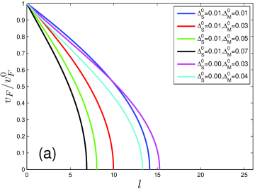
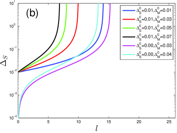
Figure 9: Flowing behavior of the parameters $v_{F}$, $\Delta_{S}$, $\Delta_{V}$, and $\Delta_{M}$ in case the system contains multi-type of disorders, where $\Delta_{V}^{0}=0.01$. The runaway behaviors of $\Delta_{S}$, $\Delta_{V}$, and $\Delta_{M}$ are not quantitatively reliable, but should be regarded as a signature of the dominance of random chemical potential in the low-energy region.

V.4 Coexistence of two or three types of disorder

In this subsection, we consider the mutual influence between distinct types of disorder. The full set of RG equations are already given by Eqs. (48)-(52), and can be solved self-consistently. For different initial conditions, the solutions are presented in Fig.9.

As shown in Fig. 9(a), the fermion velocity $v_{F}$ always flows to zero at some particular energy scale. According to Fig. 9(b) and (c), $\Delta_{S}$ and $\Delta_{V}$ increase with lowering energy scale monotonously, and appear to diverge at a finite energy scale. From Fig. 9(d), we see that $\Delta_{M}$ increases with lowering energy scale monotonously if $\Delta_{M}^{0}<2\Delta_{V}^{0}$, but displays a non-monotonic dependence on energy scale if $\Delta_{M}^{0}>2\Delta_{V}^{0}$. An important fact is that, once more than one types of disorder coexist, the three parameters $\Delta_{S}$, $\Delta_{M}$, an $\Delta_{V}$ all flow to strong couplings inevitably at low energies. This clearly informs us that distinct types of disorder are strongly correlated with each other, as can be seen from Fig. 9.

When the disorder strength flows to the strong coupling regime, it is usually believed that such behavior leads to a finite zero-energy DOS $\rho(0)\neq 0$ and a finite scattering rate, which drives the Dirac fermions to enter into a diffusive phase. As just discussed, the perturbative RG expansion method becomes out of control. In this case, one may attempt to study the effects of disorder on superconductivity by carrying out a mean-field analysis Sondhi13 . For instance, it would be possible to derive the superconducting gap equation after properly taking into account the impact of disorder. This approach has been extensively investigated in conventional dirty superconductors, and naturally leads to Anderson theorem. However, 2D Dirac semimetals exhibit interesting new features comparing to 3D ordinary metals, and one needs to be careful in the derivation of gap equation. This issue will be discussed in more detail in the next section.

V.5 Effects of ZS and ZS’ diagrams

We have elucidated in Sec. III that the contributions of ZS and ZS’ diagrams can be approximately neglected in the low-energy regime. That consideration applies only to the clean limit. We now incorporate the contributions of ZS and ZS’ diagrams into the RG equations and estimate their effects in the presence of disorders.

After including ZS and ZS’ diagrams, the RG equations of $v_{F}$ and $v_{\Gamma_{i}}$ are still given by Eqs. (48)-(51), but the RG equation for $u$ should be modified. If the system contains only random mass, we have

$$\frac{du}{dl}=-\left[1+\Delta_{M}+\frac{u[1+2(1-f^{\prime}_{Q})]}{8\pi v_{F}}\right]u,$$

where $f^{\prime}_{Q}\equiv\frac{2-2(1-\delta)^{\frac{3}{2}}}{3\delta}$. If the system contains only random gauge potential, one simply replaces $\Delta_{M}$ with $2\Delta_{V}$. We only consider the case that random mass or random gauge potential exists alone, since otherwise the perturbative RG method would be out of control. The numerical RG solutions suggest that a large value of $\delta$ favors superconductivity, whereas a small $\delta$ disfavors superconductivity. The influence of ZS and ZS’ diagrams are determined by the value of transferred momenta $Q$. Disorder effects are dominant for small $Q$, but ZS and ZS’ contributions become prevailing for large $Q$. In the RG analysis, we eventually would take $Q$ to vanish in the lowest-energy limit, which corresponds to $\delta\rightarrow 0$. In this limit, the contributions of ZS and ZS’ diagrams become progressively unimportant.

VI Further discussions about disorder effects

The impact of disorder on superconductivity has been extensively studied for nearly six decades, in the contexts of both conventional metal superconductors and various unconventional superconductors Anderson1959JPCS ; Gorkov08 ; LeeRMP1985 ; Balatsky06 . In particular, Anderson Anderson1959JPCS pointed out that the time-reversed exact eigenstates of electrons can still pair up in disordered metals. For an $s$-wave superconductor, one can show via gap equation calculations Gorkov08 that weak non-magnetic disorders do not affect the superconducting gap $m$ and the critical temperature $T_{c}$. In the case of 2D disordered Dirac semimetals, it should be still possible for the exact eigenstates of Dirac fermions related by time-reversal symmetry to form Cooper pairs. However, the magnitude of gap $m$ and $T_{c}$ might be influenced by disorder Sondhi13 .

When a 2D Dirac semimetal contains a weak random mass or gauge potential disorder, the time-reversal symmetry is broken Ludwig1994 . The Anderson theorem thus becomes invalid and cannot be used to determine the fate of superconductivity. We studied this issue by means of perturbative RG method in the last section, and showed that the disorder strength either flows to zero or is fixed at a small constant in the low-energy region. In both cases, the perturbative expansion is under control. It can also be deduced that the Dirac fermions remain extended. From the RG results presented in Sec.V, we know that either random mass or random gauge potential leads to suppression of superconductivity.

Random chemical potential is quite different since it preserves the time-reversal symmetry. Different from conventional $s$-wave metal superconductors, both the superconducting gap $m$ and temperature $T_{c}$ can be modified by random chemical potential. As mentioned in the last section, perturbative RG cannot be used to address this issue. A promising alternative is to perform a detailed gap equation analysis.

For conventional $s$-wave dirty superconductors, the impact of disorder on superconductivity can be investigated by using the AG diagrammatic approach Gorkov08 . This approach works as follows. When a conventional $s$-wave superconductor contains weak non-magnetic disorder, which exists as a random chemical potential, one can derive the following gap equation Gorkov08

$$m=\frac{u}{4}T\sum_{\omega_{n}}\int\frac{d^{d}\mathbf{k}}{(2\pi)^{d}}\frac{A_{3}m}{A_{1}^{2}\omega_{n}^{2}+\xi_{\mathbf{k}}^{2}+A_{3}^{2}m^{2}},$$ (77)

where $u$ is the BCS coupling constant, $m$ is the superconducting gap, $A_{1}$ is the renormalization factor of fermion energy, and $A_{3}$ is the renormalization factor of gap. In the clean limit, $A_{1}=A_{3}=0$. To integrate over $\mathbf{k}$, one usually needs to make an essential assumption that the Fermi surface is large enough such that the influence of disorder on the low-energy DOS can be neglected. In a 3D ordinary metal, this assumption is certainly satisfied, which allows one to employ the approximation

$$\int\frac{d^{3}\mathbf{k}}{(2\pi)^{3}}\rightarrow\int d\xi\rho(\xi)\rightarrow\rho(0)\int d\xi,$$ (78)

This then directly leads to the following gap equation

$$m = \frac{u}{4}T\sum_{\omega_{n}}\rho(0)\int d\xi\frac{A_{3}m}{A_{1}^{2}\omega_{n}^{2}+\xi^{2}+A_{3}^{2}m^{2}}$$ (79)

$$= \pi\frac{u}{4}T\rho(0)\sum_{\omega_{n}}\frac{A_{3}m}{\sqrt{A_{1}^{2}\omega_{n}^{2}+A_{3}^{2}m^{2}}}.$$

Within the AG formalism, one can prove that $A_{1}=A_{3}$, which immediately indicates that the disorder-induced renormalization factors $A_{1}$ and $A_{3}$ cancel each other exactly. Now the gap equation is further simplified to

$$m=\pi\frac{u}{4}T\rho(0)\sum_{\omega_{n}}\frac{m}{\sqrt{\omega_{n}^{2}+m^{2}}}.$$ (80)

This equation has precisely the same expression as that obtained in a perfectly clean $s$-wave superconductor Gorkov08 , which means that the superconducting gap is independent of weak random chemical potential.

Checking the computational process, we can see that the independence of superconductivity on disorder is based on an important assumption that weak disorder has nearly no effects on the low-energy DOS. In case this assumption is invalid, the disorder does not disappear. Different from 3D ordinary metals, 2D Dirac semimetal does not have a large Fermi surface, but has only discrete band-touching Dirac points. Near the Dirac points, the low-energy DOS of Dirac fermions depends on energy as $\rho(\omega)\propto|\omega|$, in the clean limit. In particular, $\rho(0)=0$ at the Fermi level. Once random chemical potential is added to the system, its effective strength increases monotonously in the low-energy region, which is often interpreted as the emergence of a disorder-controlled diffusive state Ludwig1994 ; Altland02 . A characteristic property of such a diffusive state is the generation of a finite zero-energy DOS, namely $\rho(0)\neq 0$. Since the zero-energy DOS is significantly altered by random chemical potential, both the gap $\Delta$ and $T_{c}$ are disorder dependent. To address this issue, we now apply the AG formalism to examine the impact of random chemical potential on superconductivity in 2D Dirac semimetal. After carrying out length calculations, we obtain two self-consistently coupled equations

$$A = \!\!1+\zeta A\ln\left(1+\frac{1}{A^{2}\omega^{2}+A^{2}m^{2}}\right),$$ (81)

$$1 = \!\!\frac{1}{2\pi}\frac{u}{u_{c}}\int_{-\infty}^{+\infty}\!\!d\omega A\ln\left(1+\frac{1}{A^{2}\omega^{2}+A^{2}m^{2}}\right),$$ (82)

where $\zeta=\frac{\Delta_{V}^{2}}{4\pi v_{F}^{2}}$. Here, the renormalization factor $A_{1}$ and $A_{3}$ are still equal, and can be universally represented by $A$ for simplicity. In the derivation of these two equations, one cannot adopt the approximation given by Eq. (78), but should integrate over momentum straightforwardly. It is apparent that the factor $A$ does not disappear and indeed satisfies two self-consistently coupled equations. The quantities $A$ and $m$ should be computed by solving these two equations simultaneously. Because the factor $A$ is induced by random chemical potential, the gap is definitely not independent of disorder.

Figure 10: (a) Dependence of $A$ on $\omega$ at different values of $\zeta$. (b) Dependence of $\omega A$ on $\omega$ at different values of $\zeta$.

Now let us solve the two coupled equations (81) and (82). As the system approaches the semimetal-superconductor QCP, i.e., $u\rightarrow u_{c}$, the superconducting gap vanishes continuously, and these equations can be simplified to

$$A = 1+\zeta A\ln\left(1+\frac{1}{A^{2}\omega^{2}}\right),$$ (83)

$$1 = \frac{1}{2\pi}\frac{u}{u_{c}}\int_{-\infty}^{+\infty}d\omega A\ln\left(1+\frac{1}{A^{2}\omega^{2}}\right).$$ (84)

The numerical solutions of these equations are depicted in Fig. 10, which shows that $\omega A$ approaches to some constant $\gamma$ in the zero-energy limit. The value of $\gamma$ is determined by the strength of random chemical potential. As $\omega$ decreases from the scale set by $\gamma$, $\omega A$ becomes a constant. If $\omega$ increases from $\gamma$, $A\rightarrow 1$. Thus, the asymptotic behavior of $A$ is approximately given by

$$A\sim\left\{\begin{array}[]{lll}\frac{\gamma}{|\omega|}&\mathrm{if}&|\omega|\ll\gamma,\\ 1&\mathrm{if}&|\omega|\gg\gamma.\end{array}\right.$$ (87)

According to this behavior, we find that the integration over $\omega$ in Eq. (84) is divergent, which indicates that

$$u_{c}\rightarrow 0.$$

This result means that an arbitrarily weak attraction is able to cause BCS pairing in the presence of random scalar potential, which can be considered as a disorder-induced enhancement of superconductivity Sondhi13 .

We show the dependence of gap $m$ on $u$ at different values of disorder strength $\zeta$ in Fig. 11. We find that for small $u$, the gap $m$ is enhanced by disorder, which is shown in Fig. 11(a). However, when $u$ is larger than some critical value, the gap $m$ is suppressed by disorder, as can be seen from Fig. 11(b). This result is qualitatively consistent with that of Potirniche et al. Sondhi14 , who studied the problem by solving self-consistent Bogoliubov-de Gennes equations.

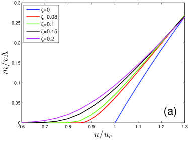
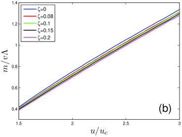
Figure 11: Dependence of gap $m$ on parameter $u$ at different values of $\zeta$.

However, we should warn that the coupled equations (81) and (82) may still be inadequate. In 3D ordinary metals, the validity of AG treatment is based on an assumption that the vertex corrections are unimportant. This assumption is justified once the inequality $k_{F}\lambda\gg 1$ is satisfied Gorkov08 . Dirac semimetals are quite different from ordinary metals since $k_{F}\rightarrow 0$, hence we can no longer utilize the condition $k_{F}\lambda\gg 1$ to judge whether the AG formalism is applicable or not. The vertex corrections may play an important role in the present system. It is an interesting task to generalize the AG approach by incorporating the vertex corrections in a self-consistent way, and examine the impact of random chemical potential on superconductivity. This will be carried out in the future work.

If random chemical potential coexists with random mass or random gauge potential, or if all the three types of disorder are present, the disorder strength parameters flow inevitably to strong couplings Foster12 , and the perturbative RG method is unable to provide a reliable tool for the determination of the fate of superconductivity in the low-energy regime. This issue might also be addressed by a proper generation of the AG diagrammatic approach. At first glance, this situation seems to be quite similar to the case in which random chemical potential exists alone. However, they are actually different. The time-reversal symmetry is preserved when the system contains only random chemical potential, but is explicitly broken once random mass and/or random gauge potential exist Evers08 ; Mirlin2006PRB ; Foster12 . It would be interesting to study whether such symmetry breaking has a remarkable impact on superconductivity.

VII Summary and discussion

In this paper, we have studied the interplay between an effective BCS-type interaction and fermion-disorder coupling by performing a RG analysis. Our main finding is that random mass and random gauge potential both lead to certain amount of increment of the critical BCS coupling $|u_{c}|$, which makes the onset of superconductivity more unlikely since a stronger net attraction is required to form Cooper pairs comparing to the clean case. In addition to the suppression of superconductivity, disorders have other drastic effects on the low-energy behaviors of Dirac fermions. At the new critical value $|u_{c}^{\prime}|$, which is lager than $|u_{c}|$ obtained in the clean limit, the system would undergo a quantum phase transition between a superconducting phase and: (a) a MFL-like phase in the case of random mass; (b) a NFL in the case of random gauge potential. It is interesting to study the critical properties of these QCPs, and examine whether an effective supersymmetry emerges in the low-energy regime.

In the case of random chemical potential, our RG analysis show that the effective disorder parameter $\Delta_{S}$ grows monotonously as energy is lowered. This indicates that such type of disorder plays a significant role at low energies, but also signals the breakdown of perturbative RG method. We have investigated the impact of random chemical potential on superconductivity by carrying out a straightforward AG analysis and compared to previous pertinent works. We then have demonstrated that such simple AG analysis might be insufficient to get a reliable conclusion and that the AG diagrammatic approach needs to be improved to include the vertex corrections self-consistently.

We also have considered the mutual influence between different types of disorder. In case more than one types of disorder coexist, all three types of disorder should be present and their effective strength parameters all flow to strong couplings Foster12 . Given that perturbative RG approach become inapplicable, other efficient theoretic techniques are urgently needed to handle this complicated problem.

We then briefly discuss the case of doped 2D Dirac semimetal. For a 2D Dirac semimetal defined at a finite chemical potential $\mu$, previous mean-field studies have found that an arbitrarily small attraction suffices to induce Cooper pairing Uchoa05 ; Kopnin08 . In light of these studies, we expect that the same conclusion should be reproduced by the RG method. In particular, the RG equation would be the same as Eq. (1). If this is the case, the critical BCS coupling should vanish: $u_{c}=0$. However, we need to emphasize that the problem of Cooper pairing becomes highly nontrivial when a 2D Dirac semimetal is doped. For the surface state of 3D topological insulator, the paring symmetry is $s$-wave at zero doping. At a finite $\mu$, the $s$-wave gap will mix with a $p_{x}+ip_{y}$-wave gap, although the $p_{x}+ip_{y}$ component is small if $\mu$ is not very large Sondhi13 . In doped graphene, the possible pairing symmetry is more complicated due to the presence of several valleys of Dirac fermions. Moreover, when graphene is doped to the vicinity of the Van Hove singularity, a $p$-wave chiral superconductivity may emerge as the ground state. Due to these complications, it is actually not easy to make a full RG analysis of superconductivity. Technically, the RG scheme used at $\mu=0$ cannot be simply applied to the case of $\mu\neq 0$. In the former case, all the associated momenta can be assumed to be small quantities in the lowest-energy limit. However, in the latter case, only the component $k_{\bot}=|\mathbf{k}|-k_{F}$ can be considered as small at low energies. To study the latter case, one should employ the RG scheme similar to that utilized in some recent works on Cooper pairing in NFL systems Metlitski15 ; Fitzptrick15 ; Raghu15 .

It is also interesting to make a RG analysis to study the impact of various types of disorder on the Cooper pairing instability in other semimetal materials, such as 3D Dirac semimetals Vafek , 2D semi-Dirac semimetals Yang14 ; Isobe16 ; Moon16 , and double- and triple-Weyl semimetals Huang16 ; Lai15 ; Jian15 .

References

- (1) R. Shankar, Rev. Mod. Phys. 66, 129 (1994).
- (2) E. Fradkin, Phys. Rev. B 33, 3263 (1986).
- (3) P. A. Lee, N. Nagaosa, and X.-G. Wen, Rev. Mod. Phys. 78, 17 (2006).
- (4) J. Orenstein and A. J. Millis, Science 288, 468 (2000).
- (5) A. H. Castro Neto, F. Guinea, N. M. R. Peres, K. S. Novoselov, and A. K. Geim, Rev. Mod. Phys. 81, 109 (2009).
- (6) V. N. Kotov, B. Uchoa, V. M. Pereira, A. H. Castro Neto, and F. Guinea, Rev. Mod. Phys. 83, 407 (2011).
- (7) S. Das Sarma, S. Adam, E. H. Hwang, and E. Rossi, Rev. Mod. Phys. 83, 407 (2011).
- (8) M. Z. Hasan and C. L. Kane, Rev. Mod. Phys. 82, 3045 (2010).
- (9) X.-L. Qi and S.-C. Zhang, Rev. Mod. Phys. 83, 1057 (2011).
- (10) O. Vafek and A. Vishwanath, Ann. Rev. Condensed Matt. Phys. 5, 83 (2014).
- (11) D. V. Khveshchenko, Phys. Rev. Lett. 87, 246802 (2001).
- (12) E. V. Gorbar, V. P. Gusynin, V. A. Miransky, and I. A. Shovkovy, Phys. Rev. B 66, 045108 (2002).
- (13) D. V. Khveshchenko and H. Leal, Nucl. Phys. B 687, 323 (2004).
- (14) G.-Z. Liu, W. Li, and G. Cheng, Phys. Rev. B 79, 205429 (2009).
- (15) G.-Z. Liu and J.-R. Wang, New J. Phys. 13, 033022 (2011).
- (16) J.-R. Wang and G.-Z. Liu, New J. Phys. 14, 043036 (2012).
- (17) B. Uchoa, G. G. Cebrera, and A. H. Castro Neto, Phys. Rev. B 71, 184509 (2005).
- (18) B. Uchoa and A. H. Castro Neto, Phys. Rev. Lett. 98, 146801 (2007).
- (19) N. B. Kopnin and E. B. Sonin, Phys. Rev. Lett. 100, 246808 (2008).
- (20) J. Gonzalez, Phys. Rev. B 78, 205431 (2008).
- (21) E. Zhao and A. Paramekanti, Phys. Rev. Lett. 97, 230404 (2006).
- (22) C. Honerkamp, Phys. Rev. Lett. 100, 146404 (2008).
- (23) B. Roy and I. F. Herbut, Phys. Rev. B 82, 035429 (2010).
- (24) B. Roy, V. Juričić, and I. F. Herbut, Phys. Rev. B 87, 041401(R) (2013).
- (25) B. Roy and V. Juričić, Phys. Rev. B 90, 041413(R) (2014).
- (26) P. Ponte and S.-S. Lee, New J. Phys. 16, 013044 (2014).
- (27) S.-K. Jian, Y.-F. Jiang, and H. Yao, Phys. Rev. Lett. 114, 237001 (2015).
- (28) W. Witczak-Krempa and J. Maciejko, Phys. Rev. Lett. 116, 100402 (2016).
- (29) R. Nandkishore, L. S. Levitov, and A. V. Chubukov, Nature Physics 8, 158 (2012).
- (30) R. Nandkishore, J. Maciejko, D. A. Huse, and S. L. Sondhi, Phys. Rev. B 87, 174511 (2013).
- (31) I.-D. Potirniche, J. Maciejko, R. Nandkishore, and S. L. Sondhi, Phys. Rev. B 90, 094516 (2014).
- (32) W. Kohn and J. M. Luttinger, Phys. Rev. Lett. 15, 524 (1965).
- (33) L. Zhao, H. Deng, I. Korzhovska, M. Begliarbekov, Z. Chen, E. Andrade, E. Rosenthal, A. Pasupathy, V. Oganesyan, and L. Krusin-Elbaum, Nature Commun. 6, 8279 (2015).
- (34) A. A. Nersesyan, A. M. Tsvelik, and F. Wenger, Nucl. Phys. B 438, 561 (1995).
- (35) A. Altland, B. D. Simons, and M. R. Zirnbauer, Phys. Rep. 359, 283 (2002).
- (36) A. W. W. Ludwig, M. P. A. Fisher, R. Shankar, and G. Grinstein, Phys. Rev. B 50, 7526 (1994).
- (37) T. Stauber, F. Guinea, and M. A. H. Vozmediano, Phys. Rev. B 71, 041406(R) (2005).
- (38) J. Wang, G.-Z. Liu, and H. Kleinert, Phys. Rev. B 83, 214503 (2011).
- (39) J.-R. Wang and G.-Z. Liu, Phys. Rev. B 89, 195404 (2014).
- (40) P. W. Anderson, J. Phys. Chem. Solids 11, 26 (1959).
- (41) L. P. Gor’kov, in Superconductivity: Conventional and Unconventional Superconductors, edited by K. H. Bennemann and J. B. Ketterson, (Spriner-Verlag, Berlin, 2008).
- (42) F. Evers and A. D. Mirlin, Rev. Mod. Phys. 80, 1355 (2008)
- (43) P. M. Ostrovsky, I. V. Gornyi, and A. D. Mirlin, Phys. Rev. B 74, 235443 (2006).
- (44) K. Nomura, M. Koshino, and S. Ryu, Phys. Rev. Lett. 99, 146806 (2007).
- (45) S. Ryu, A. P. Schnyder, A. Furusaki, and A. W. W. Ludiwig, New. J Phys. 12, 065010 (2010).
- (46) N. M. R. Peres, Rev. Mod. Phys. 82, 2673 (2010).
- (47) E. R. Mucciolo and C. H. Lewenkopf, J. Phys. Condens. Matter 22, 273201 (2010).
- (48) J. C. Meyer, A. K. Geim, M. I. Katsnelson, K. S. Novoselov, T. J. Booth, and S. Roth, Nature 446, 60 (2007).
- (49) T. Champel and S. Florens, Phys. Rev. B 82, 045421 (2010).
- (50) S. V. Kusminskiy, D. K. Campbell, A. H. Castro Neto, and F. Guinea, Phys. Rev. B 83, 165405 (2011).
- (51) S. F. Edwards and P. W. Anderson, J. Phys. F 5, 965 (1975).
- (52) I. V. Lerner, in Proceedings of the International School of Physics, Enrico Fermi Course CLI, edited by B. Altshuler and V. Tognetti (IOS Press, Amsterdam, 2003).
- (53) I. F. Herbut, V. Juricic, and O. Vafek, Phys. Rev. Lett. 100, 046403 (2008).
- (54) P. Goswami and S. Chakravarty, Phys. Rev. Lett. 107, 196803 (2011).
- (55) B. Roy and S. Das Sarma, Phys. Rev. B 90, 241112(R) (2014).
- (56) J. Wang, Phys. Lett. A 379, 1917 (2015).
- (57) B. Roy and S. Das Sarma, Phys. Rev. B 94, 115137 (2016).
- (58) B. Roy, V. Jurii, and S. Das Sarma, Sci. Rep. 6, 32446 (2016).
- (59) Y. Huh and S. Sachedv, Phys. Rev. B 78, 064512 (2008).
- (60) I. L. Aleiner and K. B. Efetov, Phys. Rev. Lett. 97, 236801 (2006).
- (61) M. S. Foster and I. L. Aleiner, Phys. Rev. B 77, 195413 (2008).
- (62) M. S. Foster, Phys. Rev. B 85, 085122 (2012).
- (63) J.-R. Wang, G.-Z. Liu, and C.-J. Zhang, New J. Phys. 18, 073023 (2016).
- (64) P. A. Lee and T. V. Ramakrishnan, Rev. Mod. Phys. 57, 287 (1985).
- (65) A. V. Balatsky, I. Vekhter, and J.-X. Zhu, Rev.Mod. Phys. 78, 373 (2006).
- (66) M. A. Metlitski, D. F. Mross, S. Sachdev, and T. Senthil, Phys. Rev. B 91, 115111 (2015).
- (67) A. L. Fitzpatrick, S. Kachru, J. Kaplan, S. Raghu, G. Torroba, and H. Wang, Phys. Rev B 92, 045118 (2015).
- (68) S. Raghu, C. Torroba, and H. Wang, Phys. Rev. B 92, 205104 (2015).
- (69) B.-J. Yang, E.-G. Moon, H. Isobe, and N. Nagaosa, Nature Phys. 10, 774 (2014).
- (70) H. Isobe, B.-J. Yang, A. Chubukov, J. Schmalian, and N. Nagaosa, Phys. Rev. Lett. 116, 076803 (2016).
- (71) G. Y. Cho and E.-G. Moon, Sci. Rep. 6, 19198 (2016).
- (72) S.-M. Huang, S.-Y. Xu, I. Belopolski, C.-C. Lee, G. Chang, T.-R. Chang, B. Wang, N. Alidoust, G. Bian, M. Neupane, D. Sanchez, H. Zheng, H.-T. Jeng, A. Bansil, T. Neupert, H. Lin, and M. Z. Hasn, Proc. Natl. Acad. Sci. U.S.A. 113, 1180 (2016).
- (73) H.-H. Lai, Phys. Rev. B 91, 235131 (2015).
- (74) S.-K. Jian and H. Yao, Phys. Rev. B 92, 045121 (2015).