Numerical simulations of Kelvin-Helmholtz instability: a two-dimensional parametric study

Abstract

Using two-dimensional simulations, we numerically explore the dependences of Kelvin-Helmholtz instability upon various physical parameters, including viscosity, width of sheared layer, flow speed, and magnetic field strength. In most cases, a multi-vortex phase exists between the initial growth phase and final single-vortex phase. The parametric study shows that the evolutionary properties, such as phase duration and vortex dynamics, are generally sensitive to these parameters except in certain regimes. An interesting result is that for supersonic flows, the phase durations and saturation of velocity growth approach constant values asymptotically as the sonic Mach number increases. We confirm that the linear coupling between magnetic field and Kelvin-Helmholtz modes is negligible if the magnetic field is weak enough. The morphological behaviour suggests that the multi-vortex coalescence might be driven by the underlying wave-wave interaction. Based on these results, we make a preliminary discussion about several events observed in the solar corona. The numerical models need to be further improved to make a practical diagnostic of the coronal plasma properties.

1 Introduction

The velocity shear concentrating in a thin layer is ubiquitous in natural flows. Under certain circumstance, the velocity shear is susceptible to the Kelvin-Helmholtz (KH) instability, and may eventually develop into turbulence or large-scale wavy motions. The KH instability is a very important mechanism for momentum and energy transport and mixing of fluid. The phenomena akin to KH instability are frequently observed in the atmosphere of planets, magnetosphere boundary, and low solar corona. For instance, ripples at the prominence surface (Ryutova et al. 2010), billows on the flank of a coronal mass ejecta (CME) (Foullon et al. 2011), and traveling fluctuations at the boundaries of the magnetic structures (Ofman & Thompson 2011; Möstl et al. 2013), were attributed to the KH instability. Plasma blobs emerging from the cusps of quiescent coronal streamers have also been interpreted as the result of nonlinear development of streaming KH instability (Chen et al. 2009).

A comprehensive understanding of the KH instability is useful for diagnosing the plasma conditions of the occurring sites. Linear analysis gave the onset condition of the KH instability in magnetized plasma (e.g., Chandrasekhar 1961),

$$[\vec{k}\cdot(\vec{u_{1}}-\vec{u_{2}})]^{2}>\frac{\rho_{1}+\rho_{2}}{\mu_{0}\rho_{1}\rho_{2}}[(\vec{k}\cdot\vec{B_{1}})^{2}+(\vec{k}\cdot\vec{B_{2}})^{2}],$$ (1)

where subscripts indicate the quantities of either side of the velocity shear. $\vec{k}$, $\vec{u}$, $\rho$, $\vec{B}$, $\mu_{0}$ are the wave vector, velocity, density, magnetic field, and permeability in vacuum, respectively. This criterion is obtained based on the assumption that the sheared layer is infinitely thin and the fluid is incompressible. Miura & Pritchett (1982) showed that compressibility can stabilize KH modes and the finite thickness of velocity shear $\Delta$ acts as a filter, e.g., only modes with $k\Delta<2$ are unstable and the fastest growing modes are those with $k\Delta\sim 0.5-1$. Wu (1986) compared the growth rate of convective and periodic KH instability and found no difference in the linear stage.

Criterion (1) and many other studies indicate that the component of magnetic field parallel to the flows can stabilize KH modes. If magnetic reconnection is taken into account, the situation is more complicated. Chen et al. (1997) studied the coupling between KH and tearing instability. No linear interaction has been confirmed. Nykyri & Otto (2001) numerically investigated the mass transport due to reconnection in KH vortices. They found that reconnection would cause the high density plasma filaments detached from the magneto-sheath. Similar numerical simulations (e.g., Otto & Fairfield 2000 and Nykyri et al. 2006) have been performed to identify and reproduce the processes which cause the fluctuations at the boundary between magnetosphere and magneto-sheath observed in-situ.

Based on the detailed observational analysis of Foullon et al. (2013), Nykyri & Foullon (2013) conducted a magnetic seismology study to parametrically determine the field configuration in the CME reconnection outflow layer. Since the magnetic flux rope could be a component of CME, the KH instability at a cylindrical surface is of particular interests. Zhelyazkov et al. (2015a, b) showed that the KH wave observed in CME is the $m=-3$ MHD mode in the twisted flux tube, where $m$ is the azimuthal wave number. Using a two-fluid approximation, Martínez-Gómez et al. (2015) studied the effects of partial ionization in cool and dense magnetic flux tubes.

Frank et al. (1996), Jones et al. (1997), Jeong et al. (2000), and Ryu et al. (2000) carried out a series of numerical simulations of the KH instability. The control parameters they used are magnetic field strength, magnetic field orientation, the sheared magnetic fields, and the perturbation from third dimension. They found that in the hydrodynamic case, the KH vortex persisted until the viscosity dissipated it. In the case with magnetic field, they classified four parameter regimes: the dissipative, disruptive, nonlinearly stable, and linearly stable regime. If the field strength is less than $\sim 0.1$ of the critical value needed for linear stabilization, the role of magnetic field is to enhance the rate of energy dissipation. The magnetic tension force in stronger field cases would disrupt the KH vortex. For magnetic field strength slightly weaker than required for linear instability, the magnetic tension enhanced during linear growth phase prevents the flow from developing into nonlinearly unstable state. In the linearly stable regime, only very small amplitude fluctuations present. Jones et al. (1997) carefully designed a set of numerical experiments to show that the magnetic field component perpendicular to the flow affects the KH instability only through minor pressure contributions and the flows are essentially two-dimensional (2D). Three-dimensional (3D) numerical simulations indicate that the KH vortex has a quasi-2D structure at the beginning. For weak magnetic fields, the 3D KH instability will eventually develop into decaying turbulence. If the magnetic field is relatively strong, the flows will undergo reorganization and become stable. Malagoli et al. (1996) identified three stages in the evolution of KH instability for marginally supersonic weak field case, namely, a linear stage, a dissipative transient stage, and a saturation stage.

In most of the earlier simulations, only the dependence of single-vortex dynamics on magnetic field configuration was parametrically studied and the sonic Mach number was fixed. The discussions about viscosity, width of velocity shear, and multiple vortices interaction in these literatures are limited. In the present study, besides magnetic field strength, we systematically explore the viscosity, width of velocity shear, and flow speed in a wide range of values. We are interested in not only the vortex dynamics but also some direct observable quantities, e.g., the duration of evolution phases. As expected, we repeat many aspects of the existing studies. We also obtain some new results that are discrepant and complementary to the earlier investigations.

In the aforementioned KH instability studies, the geometry configuration of sheared layer is simply an interface. Another type of configuration, which could mimic streamer or jets, has also been considered in some investigations (e.g., Min 1997; Zaliznyak et al. 2003; Bettarini et al. 2006, 2009). Here we only consider the interface geometry in a 2D computational domain.

The rest of this paper is organized as follows. Section 2 describes the numerical model. Section 3 presents the results from numerical simulations. In section 4, we discuss the applications of our results to the observations in solar corona. Section 5 summarizes and concludes this paper.

2 Numerical model

We numerically solve the following resistive MHD equations using the PENCIL CODE, which is an open source, modular high-order finite difference code. It is of sixth-order accuracy in space and third-order in time by default.

$$\partial\ln{\rho}/\partial t = -\vec{u}\cdot\nabla\ln{\rho}-\nabla\cdot\vec{u},$$ (2)

$$\partial\vec{u}/\partial t = -\vec{u}\cdot\nabla\vec{u}-c^{2}_{s}\nabla(s/c_{p}+\ln{\rho})$$ (3)

$$+\nu(\nabla^{2}\vec{u}+\nabla\nabla\cdot\vec{u}/3+2\vec{\Sigma}\cdot\nabla\ln{\rho})$$

$$+\zeta\nabla\nabla\cdot\vec{u}+\vec{j}\times\vec{B}/\rho,$$

$$\partial s/\partial t = -\vec{u}\cdot\nabla s+1/(\rho T)(\nabla\cdot(K\nabla T)$$ (4)

$$+2\rho\nu\vec{\Sigma}\otimes\vec{\Sigma}+\zeta\rho(\nabla\cdot\vec{u})^{2}$$

$$+\eta\mu_{0}\vec{j}^{2}),$$

$$\partial\vec{A}/\partial t = \vec{u}\times\vec{B}-\eta\mu_{0}\vec{j},$$ (5)

where $c_{s}$ is the sound speed, $c_{p}$ the specific heat at constant pressure, $s$ the specific entropy, $\vec{j}=\nabla\times\vec{B}/\mu_{0}$ the electric current density, $\vec{\Sigma}$ the rate-of-shear tensor that is traceless, $\nu$ the kinematic viscosity, $\zeta$ the bulk viscosity, $K$ the thermal conductivity, $\vec{A}$ the vector potential, and $\eta$ the magnetic resistivity. Other symbols have their standard meanings.

We consider periodic flows in the x-y plane. An ideal gas is confined in a rectangular computational domain, with $x\in[-2L,2L]$, $y\in[0,4L]$. Periodic boundary conditions are used at the y boundaries. Open boundary conditions are applied to the x boundaries. All the simulations are performed on a $512\times 512$ mesh.

The background plasma is uniform in density $\rho_{0}$ and specific entropy $s_{0}$. A velocity shear layer with hyperbolic tangent profile is initially centered at the y axis ($x=0$), i.e.,

$$u_{y}=\frac{1}{2}u_{0}(1+\tanh{\frac{x}{a}}),$$ (6)

where $a$ is the half width of the sheared layer, and $u_{0}$ is the initial flow speed. A small perturbation is introduced to $u_{x}$ at $t=0$ of the form

$$u_{x}=u^{\prime}_{x0}(e^{-\frac{(y-y_{1})^{2}}{\Delta_{y}^{2}}}-e^{-\frac{(y-y_{2})^{2}}{\Delta_{y}^{2}}}),$$ (7)

where $u^{\prime}_{x0}$ is the amplitude of perturbation, $y_{1}$, $y_{2}$, and $\Delta_{y}$ define its location and width along the y-direction. For magnetized case we impose a uniform magnetic field parallel to the initial velocity, i.e., $B_{y}=B_{0}$.

We choose a case with parameters of moderate value as our reference model. Then we vary the control parameters to check their influence on the dynamics of KH instability. For the reference model, $\rho_{0}=1$ and the magnetic field is absent. The plasma stays still in the left half computational domain ($x<0$) and flows with $u_{0}=0.5$ in the right half ($x>0$). The initial entropy is set so that $c_{s}=1.29$, and thus we have $Ma=u_{0}/c_{s}\simeq 0.39$. With $a=0.05L$, there are nearly $7$ grids in the sheared layer.

Dimensionless quantities, namely the thickness of the sheared layer $a/L$, sonic Mach number $Ma=u_{0}/c_{s}$, Alfvénic Mach number $M_{A}=u_{0}/c_{a}$, plasma beta $\beta=p_{g}/p_{m}$ , Reynolds number $Re=u_{0}L/\nu$, magnetic Reynolds number $Rm=u_{0}L/\eta$, and Péclet number $Pe=c_{p}\rho u_{0}L/K$, are used to characterize the simulation runs. Considering the stabilization due to magnetic field, only the component parallel to the flows takes effect. Therefore, it is useful to define an effective Alfvénic Mach number and an effective plasma $\beta$ with $M_{A,y}=u_{0}\sqrt{\mu_{0}\rho}/B_{y}$ and $\beta_{y}=2\mu_{0}p_{g}/B_{y}^{2}$.

The reference model is labeled as Run A and listed in Table 1 among other representative cases. In all runs presented here, we adopt $Pe=10^{6}$ and $Rm=5\times 10^{7}$. The ranges of other parameters are listed in the last column of Table 2.

Table 1: Representative simulation runs.

Run	$a/L$	$Ma$	$M_{A,y}$	$Re$	$\beta_{y}$
A	$0.05$	$0.39$	$--$	$2500$	$--$
B	$0.1$	$0.39$	$--$	$2500$	$--$
C	$0.05$	$0.39$	$--$	$250$	$--$
D	$0.05$	$0.04$	$--$	$2500$	$--$
E1	$0.05$	$0.39$	$50$	$2500$	$20000$
E2	$0.05$	$0.39$	$3.57$	$2500$	$102$
E3	$0.05$	$0.39$	$2.5$	$2500$	$50$
E4	$0.05$	$0.39$	$2.27$	$2500$	$41.3$

3 Results

Figure 1(a) shows the time evolution of $\max{(u_{y})}$ in the reference Run A, from which we can see that the evolution consists three phases: (i) an initial growth phase, in which the perturbed flow grows until the vortex starts to form; (ii) a multi-vortex stage, in which multiple fully developed KH vortices coexist until they start to merge; and (iii) a single-vortex stage, in which the single-vortex resulted from multi-vortex coalescing spins until the end of the simulation. Some control parameters can dramatically affect the dynamics of the KH vortex.

The influence of magnetic field is shown in the panel (b) of Fig. 1, where the disruption effect of very weak field and stabilization effect of strong field are evident.

In the remainder of this section, besides vortex dynamics, we inspect the parametric behaviour of evolutionary phase durations. The first peak in the evolutionary curve of $\max{(u_{y})}$ marks the saturation of the velocity growth. We define the occurrence of this local maximum as the end of initial growth phase. The duration of multi-vortex phase, $\Delta t_{mult}$, is defined as the time interval between the KH vortices evidently form and they start to coalesce.

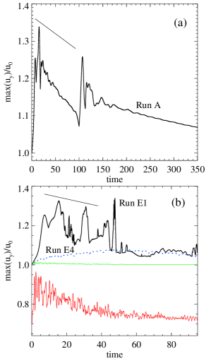
Figure 1: Evolution of $\max{(u_{y})/u_{0}}$ in typical cases. (a) hydrodynamic case (Run A); (b) thick solid black line, dotted blue line, and thin solid green line represent very weak field case (Run E1), the critical case for linear stability (Run E4), and strong field case, respectively. Oblique straight lines indicate the multi-vortex phase in Run A and Run E1. The bottom red curve in (b) is the green line shifted downward and multiplied by a factor of 20 to reveal the small-amplitude fluctuations.

3.1 Initial growth phase

The initial growth phase can be roughly divided into two stages, i.e., a linear stage followed by a nonlinear stage. The KH vortex only starts to form in the late nonlinear stage. In this stage the growing amplitude of velocity is comparable to the background flow speed, and thus the nonlinear effects cannot be ignored anymore.

Figure 2 shows the dependence of initial growth duration, $\Delta t_{init}$, on the control parameters. Viscosity and the width of sheared layer can affect considerably the initial growth time-scale. It is expected that the flow speed is critical to $\Delta t_{init}$. But this is true only for the subsonic flows ($Ma\lesssim 0.5$). It is interesting to notice that $\Delta t_{init}$ is slightly dependent on the speed of supersonic flows and approaches a constant as sonic Mach number increases (see Fig. 2(e)). As represented by the critical case in the panel (b) of Fig. 1, the initial growth phase can be hardly identified in the presence of strong magnetic field. Figure  2(g) shows that the initial growth duration measured in the weak field cases only slightly depend on the magnetic field strength. The reason may lie in the fact that the KH modes are stabilized by magnetic tension force. During the initial growth phase, especially the linear stage, there is no obvious vortex formed, and thus no Maxwell stress is induced by magnetic field distortion. So the strength of weak magnetic field plays a minor role in determining $\Delta t_{init}$. It should be pointed out that here we only talk about the growth of velocity. By contrast, the growth of magnetic field is sensitively dependent on the initial strength.

Figure 2: Phase durations and velocity saturation as a function of various parameters. Stars: velocity saturation which is measured by the first peak value of $\max{(u_{y})}$; diamonds: the duration of multi-vortex phase; triangles: the duration of initial growth phase. Note that the period of multi-vortex phase is multiplied by a factor of 1/15. In order to linearly space the data points, we plot the curves against $1/Re$ instead of $Re$ in panel (a) and (b), and against initial magnetic field strength $B_{0}$ instead of plasma $\beta$ in panel (g) and (h).

Both $u_{x}$ and $u_{y}$ are enhanced continuously by Reynolds stress during the initial growth phase. Panels on the right of Fig. 2 show the value of the first peak of $\max(u_{y})$ in its evolution curve as a function of various parameters. For the present study, in many cases the saturation of velocity enhancement is between $15\%$ and $30\%$ of the background flow speed. The first peak decreases monotonically as a function of viscosity and magnetic field strength. We identify a parameter range, $0.1\lesssim a/L\lesssim 0.2$, in which the first peak varies slightly. Compare the panel (e) and (f) in Fig. 2, we can see the similarity between $\Delta t_{init}$ and $\max(u_{y})/u_{0}$. The first peak of $\max(u_{y})/u_{0}$ is nearly independent on $Ma$ for supersonic flow and approaches an asymptotic upper limit of $\sim 1.27$ as the sonic Mach number increases.

3.2 Multi-vortex phase

The number of KH vortex is determined by the initial perturbation. In our models, two Gaussian perturbations with half width of $0.1L$ are introduced. After the initial growth, the KH vortex with $\lambda=2L$ form and evolve to $\lambda=4L$ later on. The multi-vortex phase can also be defined as the evolutionary phase with $\lambda=2L$. Figure 3 and Figure 4 show the snapshots of selected typical cases during the multi-vortex phase. The parameters used in these runs are given in Table 1.

In the present simulations, there are two fully developed vortices in most of the runs. The coexisting vortices are generally different in appearance. For example, in the reference Run A, the relatively round vortex resembles the ‘yin-yang symbol’ in Chinese traditional philosophy and the more oval vortex looks just like Cat’s Eye. Inspection reveals that the ‘yin-yang symbol’ is resulted from pairing process. We will discuss this issue in the next subsection. If the sheared layer is moderately wide ($a/L=0.1$), these two vortices are similar to each other (see Run B). In a thinner sheared layer model ($a/L=0.01$), both vortices have the appearance of ‘yin-yang symbol’. Under certain conditions, for instance, the flow is very viscous (see Run C), very slow (see Run D) or the velocity shear is very wide ($a/L\gtrsim 0.2$), the ‘yin-yang symbol’ vortex cannot develop.

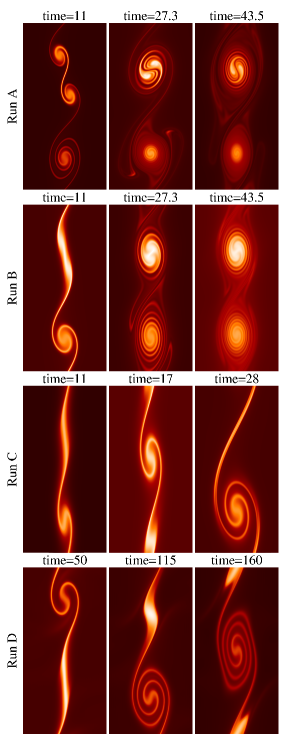
Figure 3: Snapshots of specific entropy taken during multi-vortex evolving phase for selected cases, i.e., Run A (the reference case), Run B (with wider sheared layer width), Run C (with larger viscosity) and Run D (with smaller sonic Mach number).

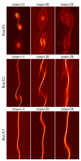
Figure 4: Snapshots of specific entropy taken during multi-vortex evolving phase for selected cases with different effective Alfvénic Mach number. Run E1: $M_{A,y}=50$; E2: $M_{A,y}=3.75$; E3: $M_{A,y}=2.5$.

The multiple vortices spin until they merge into a single vortex. Figure 2 also shows the estimated durations of multi-vortex phase. Note that in some cases, the multi-vortex phase cannot be clearly identified. The time-scale of multi-vortex phase is very sensitive to the parameter ranges explored in the current study, except for $Re\sim 1000$ and $a/L\sim 0.08$. Usually the multi-vortex phase lasts longer than the initial growth phase but an exception exists for $a/L\gtrsim 0.15$. For supersonic flows, the multi-vortex phase duration $\Delta t_{mult}$ approaches asymptotically a constant just like $\Delta t_{init}$.

The presence of magnetic field alters dramatically the KH vortex patterns, and thus the multi-vortex phase is recognizable only if the magnetic field is sufficiently weak (see Fig. 2(g)). Compared to the hydrodynamic case, the presence of magnetic field can speed up the multi-vortex phase by a factor of 2 in the very weak field case ($\beta_{y}\sim 20000$). The multi-vortex phase duration decreases as the magnetic field strength increases.

3.3 Multi-vortex coalescing

It has been pointed out that coexisting KH vortices would merge (e.g., Frank et al. 1996) and the vortex pairing process transfers energy from short wavelength to long wavelength perturbations (e.g., Malagoli et al. 1996). The present numerical simulations show that the KH vortices merge through pairing or wrapping process. Figure 5 shows the typical coalescing processes for selected cases.

Pairing takes place at the beginning stage of multi-vortex evolution phase. Top panels of Fig. 5 show that two newborn vortices rotate symmetrically around each other during pairing process. Eventually, a bigger vortex forms in the shape of ‘yin-yang symbol’. The two engaged vortices are symmetric through the period of pairing.

The merging case 1 in Fig. 5 represents a typical wrapping process. Wrapping happens near the end of the multi-vortex evolution. During the wrapping process, the Cat’s Eye eddy shrinks continuously and then is wrapped to the ‘yin-yang symbol’ eddy. The resulted single-vortex is bigger and more complicated in the fine structure. The Cat’s Eye eddy becomes a part of the perimeter structure. The merging case 2 in Fig. 5 is a special wrapping process occurring in the very viscous flows. In this case, the ‘yin-yang symbol’ vortex cannot develop and the shearing layer outside the Cat’s Eye vortex is wide at first. During the course of merging, the outside shearing layer becomes thinner and is finally wrapped to the Cat’s Eye vortex rapidly. Afterwards, the size of the Cat’s Eye is doubled and comparable to the computational domain.

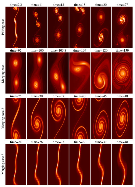
Figure 5: Coalescing processes taking place at different stages in the typical cases. Top panels: pairing process at the beginning of multi-vortex phase in Run A; Merging case 1: wrapping process at the end of multi-vortex phase in Run A; Merging case 2: merging process in Run C, where the ‘yin-yang symbol’ vortex cannot develop; Bottom panels: merging of the wavy motion in Run E3.

As long as the vortex formation is suppressed by the magnetic tension force, the KH instability develops into wavy motions. The merging case 3 in Fig. 5 can be regarded as a process of ‘multi-vortex coalescing’ in this special circumstance. During the coalescing course, the wave-like motion with wavelength $\lambda=2L$ evolves into larger structure with $\lambda=4L$ (see Run E3). Comparing these different merging cases, we may postulate that the multi-vortex coalescing is driven by the underlying wave-wave interaction. When the vortex is the dominant feature of the KH instability, the coalescing process is manifested by the complicated vortex dynamics.

3.4 Role of uniform magnetic field

The effects of magnetic field on the KH instability have been studied intensively with numerical simulations and theoretical analyses. Most of the numerical simulations were conducted for weak or very weak fields. The present study reproduces many aspects of these results (see Fig. 1(b)). Here we present some discrepant and supplementary results.

We numerically determine the onset condition for the MHD KH instability. The critical Alfvénic Mach number is $M_{A,y}\sim 2.27$, which is a little bit larger than the theoretical value $2$. The theoretical prediction is based on several assumptions; for instance, the fluid is imcompressible and the sheared layer is infinitely thin. Since the compressbility and finite width stabilize the KH modes, a little bit larger numerical value is expected. The Alfvénic Mach number can be expressed in term of sonic Mach number and plasma $\beta$, i.e., $M_{A,y}\propto Ma\sqrt{\beta_{y}}$. We conduct a numerical experiment by varying simultaneously $Ma$ and $\sqrt{\beta_{y}}$, and keeping their product unchanged. The results confirm that the linear stability is indeed determined by Alfvénic Mach number instead of plasma $\beta$. This supports the argument that the competition between Maxwell stress and Reynolds stress dominates the fate of the KH vortices.

The very weak field dissipative case ($M_{A,y}=50$, $\beta_{y}=20000$) in the present study is different from previous study, for example, the simulations done by Jones et al. (1997) and Jeong et al. (2000). In their study ($\beta=3000$ and $\beta=24000$), the KH vortex persists until viscosity and small-scale magnetic reconnection dissipate it. In our case, the KH vortex starts being destroyed soon after the small-scale magnetic reconnection taking place, as indicated by the top panels in Fig. 4. A possible explanation is that the numerical dissipation is significantly different in different MHD code. A large dissipation smooths small-scale structures quickly, and thus stops the small-scale magnetic reconnection before it dramatically disrupts the vortex. We check this effect by adopting a very large kinematic viscosity $\nu$ in one of the simulations. When the local small-scale velocity gradient is greatly reduced by viscosity, the magnetic field cannot be efficiently amplified and thus can hardly influence the flow motions. The resulted vortex dynamics nearly resembles the hydrodynamic case.

We identify a filamentary structure regime for $2.8\lesssim M_{A,y}\lesssim 6.2$ ($61\lesssim\beta_{y}\lesssim 313$). An example (Run E2) is shown in Fig. 4. In this regime, the magnetic tension force suppresses the swirling vortex when it is halfway through its first rotation. The half rolled-up vortex extends along the field lines to release its kinetic energy and the flow pattern becomes filamentary.

For the stronger field cases ($2.27\lesssim M_{A,y}\lesssim 2.8$), the KH modes cannot overcome the magnetic tension force at very beginning. The KH instability eventually develops into wavy motions (see Run E3 in Fig. 4). The wavelength of these wavy structures is finally comparable to the $y$ extent of the computational domain.

4 Discussion

Table 2: Comparison of observational and numerical non-dimensional parameters.

Parameter	F2011	O2011	M2013	F2013	Numerical
$Ma$	$0.08\sim 1.75$	$0.12\sim 0.17$	$0.66\sim 5.66$	$0.9\sim 3$	$0.05-1.5$
$M_{A}$	$0.04\sim 2.25$	$\sim 0.05$	$0.16\sim 0.68$	$1.5\sim 5$	$--$
$\beta$	$0.16\sim 2.51$	$\sim 0.15$	$\sim 0.22$	$1.5\sim 9$	$--$
$M_{A,y}$	$2.41\sim 12.98$	$\sim 5$	$0.8\sim 6.8$	$--$	$0.56-50$
$\beta_{y}$	$16\sim 854$	$\sim 1240$	$5.48\sim 21.95$	$--$	$31-20000$
$\Delta/\lambda$	$0.17\sim 0.27$	$\sim 0.11$	$0.13\sim 0.2$	$--$	$0.01-0.3$
$Re$	$--$	$--$	$--$	$--$	$250-2500$

Our results are applicable to a wide variety of astrophysical problems. In this paper, we present a preliminary application to the solar corona.

4.1 Applicability to solar corona

According to the linear analysis, the KH instability may be excited by superalfvénic flows anywhere in the solar atmosphere (Ryutova 2015). This kind of instability is actually the oscillation of flux tube. As a gas dynamics dominated structure, the classic rolled-up KH vortex can develop only if plasma $\beta$ or sonic Mach number is extremely large. Since the solar corona is highly structured and very dynamic (see Fig. 1.17 in Aschwanden 2005), the strength of magnetic field may vary considerably. If we consider the hydrostatic equilibrium, plasma $\beta$ varies much faster than magnetic field strength. The well-known coronal condition, $\beta\ll 1$, should be applied to the magnetic field dominated regions. Far from the major area of these regions, e.g., at the interface between different structures, it is possible that plasma $\beta$ is considerably larger than unit. It is probable that rolled-up KH vortex can develop at these locations during some fast transient processes.

In order to validate the application of our results to the solar corona, in Table 2, we compare the non-dimensional parameters used in the current study to that taken or roughly deduced from observations. F2011, O2011, M2013, and F2013 stand for the events that reported by Foullon et al. (2011), Ofman & Thompson (2011), Möstl et al. (2013), and Feng et al. (2013), respectively. Note that the coronal magnetic field cannot be directly measured. So the field strength and orientation presented in these observations are indeed given by rough estimates. Table 2 shows that the plasma conditions for the coronal KH instability vary dramatically from case to case, and the parameter ranges in our study at least partially overlap with the observations. Especially the effective Alfvénic Mach number lies exactly in the theoretically predicted range.

In a realistic situation, the development of KH instability is essentially a 3D problem. The numerical experiments conducted by Ryu et al. (2000) indicate that in the early stage of 3D KH instability development, 2D Cat’s Eye develops and is subsequently destroyed in all the nonlinearly unstable cases. The fully developed 3D KH instability is either decaying turbulence for weak field or become stable for strong field. The 2D rolled-up vortex is the most distinguishable feature of the KH instability and thus easily identifiable during the observation. So a 2D investigation is of practical meaning.

4.2 Evolutionary phase duration

The observed growing and evolving durations of the KH instability are significantly different. Foullon et al. (2013) estimated a period of around 2 minute between the first acceleration jet and the first perturbation appeared on the CME flank, and the evolution of visible vortices lasts about 45 seconds. Ofman & Thompson (2011) obtained a developing period of 13 minutes, and an evolving period of more than one and half hours. The event analyzed by Möstl et al. (2013) has estimated growing period of 6 minutes.

The linear growth rate of the KH mode for a plasma with uniform density is $q=\frac{1}{2}k\Delta v=\pi\Delta v/\lambda$. So provided velocity shear and wavelength, we can calculate the linear growth rate for the observed events. Table 3 contains the calculated linear growth rate and some observed properties of the coronal KH instability, where $\Delta t_{init}$ and $\Delta t_{evol}$ are the growing and evolving duration, respectively. Unless the whole growth phase is linear and the saturation of velocity is a universal constant, we cannot expect that the time-scale of initial growth is uniquely determined by the linear growth rate. In order to explain the observations we need to consider the nonlinear effect, and the results in Fig. 2 may shed light on it.

In numerical simulations we often have to adopt a Reynolds number much smaller than the realistic value by several orders of magnitude. As previously stated, the viscosity can affect the initial growth period considerably. A linear extrapolation from Fig. 2(a) suggests that $6.5\lesssim\Delta t_{init}\lesssim 6.74)$ when $Re\gtrsim 10000$. This means that if the Reynolds number is significantly large, the difference in initial growth duration caused by viscosity is extremely limited. Also, the magnetic field in the KH events observed in the low solar corona need to be weak enough so that the vortices can roll up. As mentioned in the Results section, the initial growth duration is only slightly dependent on the weak magnetic field strength. These two results suggest that among the tested parameters we should concentrate on the width of sheared layer and flow speed to explain the differences in the observed coronal KH events.

Firstly we compare the two events observed by Foullon et al. (2011) and Möstl et al. (2013). The fast flows in these two events are supersonic (see Table 2). According to the results in Fig. 2(e), the initial growth period approaches an asymptotic constant for supersonic flows. By contrast, we have $\Delta t_{init}(M2013)/\Delta t_{init}(F2011)=3$ from observations. The cause of the difference may be the width of the sheared layer. But the uncertainties in measurement prevent a deterministic comparison of the shear width in these two events. Using Fig. 2(c) we may roughly estimate that the initial growth period varies by a factor of 3 for $0.1\lesssim\Delta/\lambda\lesssim 0.3$. Since $\Delta t_{init}(M2013)>\Delta t_{init}(F2011)$, we expect that the width of velocity shear $\Delta/\lambda$ is wider in M2013.

Then we discuss the difference between F2011 and O2011. Table 2 shows that the flow speed in these two events is very different. For fast flows, $Ma(F2011)\sim 1.5$ and $Ma(O2011)\sim 0.15$. From numerical simulations (see Fig. 2(c)), we roughly have $\Delta t_{init}(Ma=0.15)/\Delta t_{init}(Ma=1.5)\sim 4.4$. From observations (see Table 2), we get $\Delta t_{init}(O2011)/\Delta t_{init}(F2011)\sim 6.5$. The observed ratio is too large compared to the numerical value. This should be from the width of sheared layer. Since a wider width causes a longer initial growth duration, we expect that $\Delta/\lambda$ is larger in O2011.

For several reasons, we cannot make a similar discussion for the multi-vortex evolutionary phase at the present stage. Firstly in the low solar corona the rapid evolution of background structure may eliminate the existing conditions, and thus terminates the KH mode before it develops into multi-vortex phase. Secondly with nowadays instruments, the fine structure of KH vortices cannot be resolved in the low solar corona and we cannot tell if a rolled-up vortex has gone through coalescing or not. Another limitation is from the numerical models. In the present study, there are only two fully developed vortices during the multi-vortex phase. In realistic situations, the train of KH vortices may undergo hierarchical merging process if the plasma conditions at the occurring place are stable. Nevertheless, a diagnostic is possible for some special cases. For example, in nonlinearly stable regime, the dynamic vortices are suppressed by magnetic field, the multi-vortex evolution can be traced by wave-wave interaction. This situation resembles somewhat the event observed by Feng et al. (2013). But their observation is made in the high corona, and the KH instability triggering event cannot be traced. There is no obvious wave-wave interaction in this event either. We will discuss this event further in the next subsection.

Table 3: Properties of observed KH instability in solar corona.

Parameter	F2011	O2011	M2013	F2013
$\Delta t_{init}$	$2m$	$13m$	$6m$	$--$
$\Delta t_{evol}$	$45$s	$>90m$	$--$	$--$
$\lambda$	$\sim 18.5\pm 0.5$Mm	$\sim 7$Mm	$\sim 14.4$Mm	$2\sim 3R_{\odot}$
$h$	$\sim 10$Mm	$--$	$2.5\sim 4$Mm	$0.3\sim 0.5R_{\odot}$
$h/\lambda$	$0.53\sim 0.56$	$--$	$0.17\sim 0.28$	$0.1\sim 0.25$
$\Delta v$	$\sim 680$km/s	$6\sim 20$km/s	$\sim 320\pm 40$km/s	$\sim 350$km/s
$q$	$0.113\sim 0.169$/s	$0.003\sim 0.009$/s	$0.061\sim 0.079$/s	$0.0005\sim 0.00075$/s

4.3 Vortex size

The height of the billow structure observed in Foullon et al. (2011) reaches $h\sim 10Mm\sim 0.5\lambda$. The vortex features observed by Ofman & Thompson (2011) are $\sim 7Mm$ in size, which is also the wavelength they assumed for analysis. The size of vortices from Möstl et al. (2013) ranges from $\sim 0.17\lambda$ to $\sim 0.28\lambda$. The amplitude of the wave-like motion observed by Feng et al. (2013) is $\sim 0.1\lambda$ and increases over the observing period. The current simulations show that for mature vortex the ratio of $h/\lambda$ varies approximately between $0.25$ and $0.5$. The discrepancy between the numerical and observed ranges (see Table 3) could be caused by the evolutionary phase difference.

The KH vortex usually has a oval shape. In some cases, it becomes relatively round right after merging, and is elongated along the velocity shear lately. In the event reported by Foullon et al. (2011), some vortices rotate about $180$ degree for $\sim 24s$ and then disappear probably due to the change of background structures. The variation of height of the KH vortices reported by Möstl et al. (2013) can be attributed to the rotation of the elliptical vortex. The identification of rotating vortices suggests that $M_{A,y}\gtrsim 6.2$ in these events, otherwise the KH modes will develop into filamentary or wavy flow motions.

The event reported by Feng et al. (2013) resembles the numerical run E3 very closely. In E3, $Ma=0.39$, $\beta_{y}=50$, and $M_{A,y}=2.5$ (see Table 1). In F2013, $Ma\sim 3$ (see Table 2). Recall that the key parameter for KH instability is the effective Alfvénic Mach number and $M_{A,y}\propto Ma\sqrt{\beta_{y}}$. Assuming the effective Alfvénic Mach number is roughly same in E3 and F2013, we can estimate that $\beta_{y}\sim 50(0.39/3)^{2}\sim 0.85$ in F2013. From observation and the general properties of the solar corona, we estimate that $1.5<\beta<9$ in F2013 (see Table 2). Considering the uncertainties in these estimations, the difference is not that large.

In run E3 the length scale of perturbation is initially $0.2L$ and increases during the development of KH instability. It reaches $\sim 2L$ in the multi-vortex phase and $\sim 4L$ after coalescing. Meanwhile, the amplitude of the wavy motion increases until it reaches $\sim 0.5L$. In F2013 the length scale and amplitude also increase continuously during the observation. Table 3 shows that the wavelength increases from $2R_{\sun}$ to $3R_{\sun}$ and the amplitude increases from $0.3R_{\sun}$ to $0.5R_{\sun}$. It seems that the variation ranges in simulation and observation are close to each other. But this is not a fair comparison due to the limitations of numerical models. In simulations the background plasma is uniform and the wavelength is restricted by the $y$ extent of the computational domain. In the solar corona the KH wavelength can increases freely and the rapid dropping of the background plasma density may cause a fast growth of the amplitude.

5 Summary and conclusion

Based on 2D numerical simulations, the dependences of KH instability on some important parameters have been investigated. The parameters that we explored are viscosity, sheared layer width, flow speed, and magnetic field strength. In the present study, we focus on the evolutionary phase duration and KH vortex morphology. The main results can be summarized as follows.

For typical hydrodynamic cases, we discern three stages in the evolution of the KH instability, i.e., a multi-vortex phase which is preceded by a monotonically growing phase and followed by a single-vortex spinning phase. The presence of magnetic field and variation of parameters may greatly affect these stages in a complicated way. For example, the initial growth time scale is sensitive to the tested parameters, but there are some regimes, such as $a/L\sim 0.2$, $Ma\gtrsim 1$, and $M_{A,y}\gtrsim 3$, in which the initial growth duration varies slightly. An interesting point from the present simulations is that for supersonic flows, the phase durations and saturation of flow growth asymptotically approach constant values as the sonic Mach number increases. Although magnetic field can dramatically alter the KH vortex morphology, the linear coupling between magnetic field and KH modes during the initial growth phase is negligible.

In many cases a KH vortex with appearance of ‘yin-yang symbol’ is formed through the pairing process. In the pairing process, two newborn vortices rotate around each other symmetrically and finally merge into one vortex. At the end of multi-vortex phase, the KH vortices coalesce through wrapping process, in which one vortex is wrapped to the other and becomes a part of the perimeter structure of the resulted single-vortex. When the formation of KH vortex is suppressed, the coalescence happens between wavy structures; therefore we may speculate that the multi-vortex coalescing is driven by underlying wave-wave interaction and manifested by vortex dynamics.

In our simulations, the MHD KH mode is linearly stable for $M_{A,y}\lesssim 2.27$. In the regime $2.27\lesssim M_{A,y}\lesssim 2.8$, the MHD KH mode is nonlinearly stable and develops into wavy motions. A weak magnetic field with $2.8\lesssim M_{A,y}\lesssim 6.2$ causes the KH mode evolving into filamentary flows. The KH vortex can roll up in an even weaker magnetic field, e.g., a case with $M_{A,y}=50$. But the small-scale reconnection can destroy the integrity of vortex soon after its formation.

As a fundamental mechanism responsible for various astrophysical phenomena, KH instability is of general interests. Based on the results from 2D numerical simulations, we make a general discussion about four events observed in solar corona. It is promising to develop a practical diagnostic tool for the coronal plasma properties. In order to do so, the current numerical KH models need to be further improved. The plasma $\beta$, sonic Mach number, width of sheared layer, and magnetic topology need to be set simultaneously according to the properties of the targeted phenomenon.

References

- Aschwanden (2005) Aschwanden, M. J. 2005, Physics of the Solar Corona. An Introduction with Problems and Solutions (2nd edition)
- Bettarini et al. (2006) Bettarini, L., Landi, S., Rappazzo, F. A., Velli, M., & Opher, M. 2006, A&A, 452, 321
- Bettarini et al. (2009) Bettarini, L., Landi, S., Velli, M., & Londrillo, P. 2009, Physics of Plasmas, 16, 062302
- Chandrasekhar (1961) Chandrasekhar, S. 1961, Hydrodynamic and hydromagnetic stability
- Chen et al. (1997) Chen, Q., Otto, A., & Lee, L. C. 1997, J. Geophys. Res., 102, 151
- Chen et al. (2009) Chen, Y., Li, X., Song, H. Q., et al. 2009, ApJ, 691, 1936
- Feng et al. (2013) Feng, L., Inhester, B., & Gan, W. Q. 2013, ApJ, 774, 141
- Foullon et al. (2011) Foullon, C., Verwichte, E., Nakariakov, V. M., Nykyri, K., & Farrugia, C. J. 2011, ApJ, 729, L8
- Foullon et al. (2013) Foullon, C., Verwichte, E., Nykyri, K., Aschwanden, M. J., & Hannah, I. G. 2013, ApJ, 767, 170
- Frank et al. (1996) Frank, A., Jones, T. W., Ryu, D., & Gaalaas, J. B. 1996, ApJ, 460, 777
- Jeong et al. (2000) Jeong, H., Ryu, D., Jones, T. W., & Frank, A. 2000, ApJ, 529, 536
- Jones et al. (1997) Jones, T. W., Gaalaas, J. B., Ryu, D., & Frank, A. 1997, ApJ, 482, 230
- Malagoli et al. (1996) Malagoli, A., Bodo, G., & Rosner, R. 1996, ApJ, 456, 708
- Martínez-Gómez et al. (2015) Martínez-Gómez, D., Soler, R., & Terradas, J. 2015, A&A, 578, A104
- Min (1997) Min, K. W. 1997, ApJ, 482, 733
- Miura & Pritchett (1982) Miura, A., & Pritchett, P. L. 1982, J. Geophys. Res., 87, 7431
- Möstl et al. (2013) Möstl, U. V., Temmer, M., & Veronig, A. M. 2013, ApJ, 766, L12
- Nykyri & Foullon (2013) Nykyri, K., & Foullon, C. 2013, Geophys. Res. Lett., 40, 4154
- Nykyri & Otto (2001) Nykyri, K., & Otto, A. 2001, Geophys. Res. Lett., 28, 3565
- Nykyri et al. (2006) Nykyri, K., Otto, A., Lavraud, B., et al. 2006, Annales Geophysicae, 24, 2619
- Ofman & Thompson (2011) Ofman, L., & Thompson, B. J. 2011, ApJ, 734, L11
- Otto & Fairfield (2000) Otto, A., & Fairfield, D. H. 2000, J. Geophys. Res., 105, 21175
- Ryu et al. (2000) Ryu, D., Jones, T. W., & Frank, A. 2000, ApJ, 545, 475
- Ryutova (2015) Ryutova, M. 2015, Physics of Magnetic Flux Tubes, doi:10.1007/978-3-662-45243-1
- Ryutova et al. (2010) Ryutova, M., Berger, T., Frank, Z., Tarbell, T., & Title, A. 2010, Sol. Phys., 267, 75
- Wu (1986) Wu, C. C. 1986, J. Geophys. Res., 91, 3042
- Zaliznyak et al. (2003) Zaliznyak, Y., Keppens, R., & Goedbloed, J. P. 2003, Physics of Plasmas, 10, 4478
- Zhelyazkov et al. (2015a) Zhelyazkov, I., Chandra, R., Srivastava, A. K., & Mishonov, T. 2015a, Ap&SS, 356, 231
- Zhelyazkov et al. (2015b) Zhelyazkov, I., Zaqarashvili, T. V., & Chandra, R. 2015b, A&A, 574, A55