Characterisation of the turbulent electromotive force and its magnetically-mediated quenching in a global EULAG-MHD simulation of solar convection

Abstract

We perform a mean-field analysis of the EULAG-MHD millenium simulation of global magnetohydrodynamical convection presented in Passos & Charbonneau (2014). The turbulent electromotive force operating in the simulation is assumed to be linearly related to the cyclic axisymmetric mean magnetic field and its first spatial derivatives. At every grid point in the simulation’s meridional plane, this assumed relationship involves 27 independent tensorial coefficients. Expanding on Racine et al. (2011), we extract these coefficients from the simulation data through a least-squares minimization procedure based on singular value decomposition. The reconstructed $\bm{\alpha}$-tensor shows good agreement with that obtained by Racine et al. (2011), who did not include derivatives of the mean-field in their fit, as well as with the $\bm{\alpha}$-tensor extracted by Augustson et al. (2015) from a distinct ASH MHD simulation. The isotropic part of the turbulent magnetic diffusivity tensor $\bm{\beta}$ is positive definite and reaches values of $5.0\times 10^{7}\,$m${}^{2}\,$s^-1 in the middle of the convecting fluid layers. The spatial variations of both $\alpha_{\phi\phi}$ and $\beta_{\phi\phi}$ component are well reproduced by expressions obtained under the Second Order Correlation Approximation, with a good matching of amplitude requiring a turbulent correlation time about five times smaller than the estimated turnover time of the small-scale turbulent flow. By segmenting the simulation data into epochs of magnetic cycle minima and maxima, we also measure $\alpha$- and $\beta$-quenching. We find the magnetic quenching of the $\alpha$-effect to be driven primarily by a reduction of the small-scale flow’s kinetic helicity, with variations of the current helicity playing a lesser role in most locations in the simulation domain. Our measurements of turbulent diffusivity quenching are restricted to the $\beta_{\phi\phi}$ component, but indicate a weaker quenching, by a factor of $\simeq 1.36$, than of the $\alpha$-effect, which in our simulation drops by a factor of three between the minimum and maximum phases of the magnetic cycle.

1 Introduction

A proper understanding of the physical mechanism(s) underlying solar dynamo action and regulating the cycle’s amplitude and duration are crucial components of long term prediction of space weather (also known as “space climate”), and of research on solar-terrestrial interaction in general (Weiss, 2010). We are still a long way from physically-based prediction of solar cycle characteristics, even though significant progress has been made in recent years (for a recent review see Petrovay 2010). Part of the difficulty lies with the fact that no concensus currently exists as to the mode of operation of the solar cycle; the shearing of the solar magnetic field by differential rotation is usually considered as a key process, but what drives the regeneration of the solar dipole moment remains ill-understood. Some dynamo models invoke the electromotive force associated with turbulent convection, others the surface decay of active regions (the Babcock-Leighton mechanism), while others yet focus on various rotationally-influenced (magneto)hydrodynamical instabilities taking place immediately beneath the base of the solar convection zone. A survey of these different types of dynamo models can be found in (Charbonneau, 2010). Such models make use of geometrical and dynamical simplifications, most notably perhaps the use of the so-called kinematic approximation, in which the dynamical backreaction of the magnetic field on the inductive flows is neglected or parametrized through largely ad hoc prescriptions. Proper tuning of these ad hoc functionals and associated model parameters can in many cases lead to cyclic behavior showing reasonably solar-like variability patterns in the amplitude and duration of magnetic cycles (see, e.g., Karak & Choudhuri (2011); Kitchatinov & Olemskoy (2012) and references therein)

An alternate approach is made possible by global magnetohydrodynamical simulations of solar convection, which recently have succeeded in producing magnetic fields well-organized on large spatial scales and undergoing more or less regular polarity reversals (Brown et al. 2010, 2011; Ghizaru et al. 2010; Käpylä et al. 2010; Racine et al. 2011; Käpylä et al. 2012; Masada et al. 2013; Beaudoin et al. 2013; Passos & Charbonneau 2014; Fan & Fang 2014; Augustson et al. 2015). There are no active regions in such simulations (but do see Nelson et al. 2013, 2014), and therefore no Babcock-Leighton mechanism, but the turbulent electromotive force associated with thermally-driven convection is captured in a dynamically consistent manner at spatial and temporal scales resolved by the computational grid. Evidence for the development of MHD instabilities has also been found in some of these simulations (see Lawson et al. 2015; Miesch 2007).

The availability of such simulation data allows to bridge the gap between simplified kinematic models and MHD simulations of solar convection. More specifically, the latter can be used to measure turbulent coefficients usually specified in largely ad hoc fashion in the former. Of particular interest is the turbulent electromotive force, its associated $\alpha$-effect and turbulent diffusivity, and variations of these as a function of the magnetic field strength. Such measurements can assist in the interpretation of simulation results, and may help in clarifying some puzzling differences in the characteristics of cycles generated by simulations that are generally alike and differ primarily in what one would have hoped are only computational and algorithmic detail (see, e.g., §3.2 Charbonneau 2014). Moreover, mean-field models incorporating source terms and physical coefficients derived from numerical simulations can be useful in exploring long timescale behaviors that remain unaccessible to full MHD simulations, due to limitations in computing resources.

The aim of this paper is twofold. First, we document and validate a generalization of the least-squares minimization technique introduced by Racine et al. (2011)(see also Brandenburg & Sokoloff 2002) for extracting mean-field coefficients from the output of global MHD simulations of solar convection. Second, we use this methodology to measure the level of magnetically-mediated quenching of the $\alpha$-effect and turbulent diffusivity operating in the simulation. Section 2 presents a minimal overview of classical mean-field electrodynamics, focusing on aspects necessary to properly frame the analyses to follow. In section 3.1 we describe the least-squares minimization method used to extract the $\bm{\alpha}$- and $\bm{\beta}$-tensors, and present the results of this procedure in §3.2 and 3.3, applied to the “millenium simulation” described in Passos & Charbonneau (2014). We also compare in §3.4 the isotropic part of these two tensors to reconstructions using analytical forms obtained under the second-order correlation approximation. In sections 4 we turn to an investigation of the magnetic suppression of the $\alpha$-effect and turbulent diffusivity. We close in §5 by summarizing our conclusions and discussing the limitation of our analyses.

2 Mean-field electrodynamics

The mathematical and physical underpinnings of mean-field electrodynamics are well-covered in many textbooks and review articles (see, e.g., Moffatt 1978; Krause & Rädler 1980; Ossendrijver 2003; Brandenburg & Subramanian 2005; Charbonneau 2010). What follows is only a brief overview, focusing on definitions and reformulations of the $\bm{\alpha}$- and $\bm{\beta}$-tensors on which the analyses presented in this paper are based. The starting point of classical mean-field electrodynamics is the separation of the magnetic field (${\bm{B}}$) and flow (${\bm{u}}$) into a spatially large-scale, slowly varying mean component, and a small-scale, rapidly varying fluctuating component:

$$\bm{u}=\langle\bm{u}\rangle+\bm{u}^{\prime},\;\;\;\bm{B}=\langle\bm{B}\rangle+\bm{B}^{\prime}~{},$$ (1)

where the prime quantities represent the fluctuating part and the brackets $\langle...\rangle$ denote an intermediate averaging scale over which the fluctuating parts vanish, i.e., $\langle\bm{u}^{\prime}\rangle=0$ and $\langle\bm{B}^{\prime}\rangle=0$. Inserting eq. (1) into the magnetohydrodynamical induction equation and applying this averaging operator yields:

$$\frac{\partial{\langle\bm{B}\rangle}}{\partial{t}}=\nabla\times\left(\langle\bm{u}\rangle\times\langle\bm{B}\rangle+\mathcal{\bm{E}}-\mathrm{\eta}\nabla\times\langle\bm{B}\rangle\right)~{},$$ (2)

where

$$\mathcal{\bm{E}}=\langle\bm{u}^{\prime}\times\bm{B}^{\prime}\rangle~{},$$ (3)

is the mean electromotive force (emf) due to the fluctuation of the flow and the magnetic field, and $\eta$ is the magnetic diffusivity. The next step is to develop this emf in terms of the mean magnetic component and its derivatives. Because we are working here with vector fields, such a development is written as:

$$\mathcal{\bm{E}}=\bm{a}\langle{\bm{B}}\rangle+\bm{b}\nabla\langle{\bm{B}}\rangle+\textrm{higher order derivatives}~{},$$ (4)

where the tensors $\bm{a}$ and $\bm{b}$ appearing in this expression are assumed to depend only on the statistical properties of the small-scale flow and field (see, e.g., Krause & Rädler 1980). Truncation of the higher order derivatives is justified provided a good separation of spatial and/or temporal scale exists between the fluctuating velocity and magnetic fields on one hand, and the large-scale magnetic and flow field on the other. The first term in the expansion involves a rank-two tensor capturing (among other effects) the so-called $\alpha$-effect, which can act as a source term in the mean-field equation (2). The second term in the series is a rank-three tensor and embodies (among other effects) the destructive action of turbulent diffusion on the mean magnetic field (see Rädler 1980, 2000; Rädler & Stepanov 2006). It is convenient —and physically meaningful— to separate out the symmetric part of these tensors, so that with the higher-order terms neglected eq. (4) can be rewritten as :

$$\mathcal{E}=\bm{\alpha}\cdot\langle{\bm{B}}\rangle+\bm{\gamma}\times\langle{\bm{B}}\rangle-\bm{\beta}\cdot(\nabla\times\langle{\bm{B}}\rangle)-\bm{\delta}\times(\nabla\times\langle{\bm{B}}\rangle)-\bm{\kappa}\cdot(\nabla\langle{\bm{B}}\rangle)^{sym}~{},$$ (5)

where

$$\alpha_{ij}={1\over 2}(a_{ij}+a_{ji})~{},\qquad\gamma_{k}=-{1\over 2}\epsilon_{kij}a_{ij}~{}.$$ (6)

The $\bm{\alpha}$-term now describes the classical $\alpha$-effect, which in the present context is related to the kinetic helicity of the unmagnetized flow, and the vectorial quantity $\bm{\gamma}$ acts on the mean field as an additional (pseudo)velocity known as turbulent pumping. The $\bm{b}$ tensor is separated into three components; a rank-two tensor $\bm{\beta}$, a vectorial quantity $\bm{\delta}$, and a rank-three tensor $\bm{\kappa}$. The first two can be interpreted as anisotropic contributions to the mean-field resistivity, and the last one embodies other more complex influences of the mean field. The $\bm{\beta}$-tensor is the symmetric part of the more general $\bm{b}$-tensor and is defined as follows:

$$\beta_{ij}={1\over 4}(\epsilon_{i\mu\nu}b_{j\mu\nu}+\epsilon_{j\mu\nu}b_{i\mu\nu})~{}.$$ (7)

Working in spherical polar coordinate ($r,\theta,\phi$) and assuming that $\langle{\bm{B}}\rangle$ varies only weakly in space and by construction is axisymmetric ($\partial{}/\partial{\phi}\equiv 0$), the emf can be rewritten as:

$$\mathcal{E}_{m}=\widetilde{a}_{mk}\langle{B_{k}}\rangle+\widetilde{b}_{mkr}\frac{\partial{\langle B_{k}\rangle}}{\partial{r}}+\frac{\widetilde{b}_{mk\theta}}{r}\frac{\partial{\langle B_{k}\rangle}}{\partial{\theta}}~{},$$ (8)

where $\widetilde{a}$ and $\widetilde{b}$ are pseudo-tensors, which can be related to the true tensors $\bm{a}$ and $\bm{b}$ by introducing proper covariant differentiation for the $\partial{\langle B_{j}\rangle}/\partial{x_{k}}$, so as to account for the curvilinear nature of the (spherical) coordinate system and its associated unit vectors. Because our adopted averaging is a zonal average, all $\partial{\langle B_{j}\rangle}/\partial{x_{\phi}}$ are zero, and consequently only 18 out of the 27 components of the $\bm{\widetilde{b}}$ pseudo-tensor are accessible (see Schrinner et al. (2007) for further details). In spherical geometry we thus have:

$$\alpha_{rr}=\widetilde{a}_{rr}-\frac{\widetilde{b}_{r\theta\theta}}{r}~{},\\$$ (9a)

$$\alpha_{r\theta}=\alpha_{\theta r}={1\over 2}(\widetilde{a}_{r\theta}+\widetilde{a}_{\theta r}+\frac{\widetilde{b}_{rr\theta}}{r}-\frac{\widetilde{b}_{\theta\theta\theta}}{r})~{},\\$$ (9b)

$$\alpha_{r\phi}=\alpha_{\phi r}={1\over 2}(\widetilde{a}_{r\phi}+\widetilde{a}_{\phi r}-\frac{\widetilde{b}_{\phi rr}}{r})~{},\\$$ (9c)

$$\alpha_{\theta\theta}=\widetilde{a}_{\theta\theta}+\frac{\widetilde{b}_{\theta r\theta}}{r}~{},\\$$ (9d)

$$\alpha_{\theta\phi}=\alpha_{\phi\theta}={1\over 2}(\widetilde{a}_{\theta\phi}+\widetilde{a}_{\phi\theta}+\frac{\widetilde{b}_{\phi r\theta}}{r})~{},\\$$ (9e)

$$\alpha_{\phi\phi}=\widetilde{a}_{\phi\phi}~{}.$$ (9f)

Note here the appearance of $\widetilde{b}$-related contributions to the $\bm{\alpha}$-tensor, a direct consequence of spatial derivatives acting on unit vectors of the spherical coordinate system. Similar expressions relating the components of $\bm{\beta}$ to those of $\bm{\widetilde{b}}$ are given by equations (12a) through (15k) in Schrinner et al. (2007), and are not replicated in full here, except for the diagonal components:

$$\beta_{rr}=-\frac{1}{2}\;\widetilde{b}_{r\phi\theta}~{},\,\,\,\,\beta_{\theta\theta}=\frac{1}{2}\;\widetilde{b}_{\theta\phi r}~{},\,\,\,\,\beta_{\phi\phi}=\frac{1}{2}(\widetilde{b}_{\phi r\theta}-\widetilde{b}_{\phi\theta r})~{}.$$ (10)

Note finally that the isotropic part of the $\bm{\beta}$-tensor, i.e.:

$$\beta\equiv{1\over 3}(\beta_{rr}+\beta_{\theta\theta}+\beta_{\phi\phi})~{},$$ (11)

corresponds to the coefficient of turbulent diffusivity introduced in the vast majority of published mean-field and mean-field-like dynamo models of the solar cycle, including those relying on inductive source terms distinct from the turbulent electromotive embodied in the $\bm{\alpha}$-tensor.

3 Extracting the $a$-and $b$-tensors

The numerical data used in what follows is taken from the EULAG-MHD “millenium simulation” described in Passos & Charbonneau (2014); (see also Ghizaru et al. 2010; Beaudoin et al. 2013; Charbonneau & Smolarkiewicz 2013; Smolarkiewicz & Charbonneau 2013). This global simulation of thermally-driven MHD convection spans 1600yr of simulated time, and generates an axisymmetric large-scale magnetic field undergoing regular polarity reversals on a $\simeq 40\,$yr cadence.

A number of distinct approaches have been designed to extract the $\bm{a}$- and $\bm{b}$-tensors from the output of MHD turbulence simulations. The test-field method (Schrinner et al. 2007, see also Käpylä et al. 2009) solves a set of evolution equations for the turbulent fluctuations ${\bm{B}}^{\prime}$ produced by the kinematic action of the flow on a set of imposed large-scale “test magnetic field”. The turbulent emf is then calculated directly via eq. (3), and with the test fields playing the role of the large-scale magnetic field $\langle{\bm{B}}\rangle$, the tensorial components of the emf development (4) can be obtained.

An alternate, direct approach is possible in the case of simulations which generate autonomously a large-scale magnetic field, as in the EULAG-MHD millenium simulation. Subtracting this large-scale field from the total magnetic field yields ${\bm{B}}^{\prime}$, and a similar procedure applied to the total flow provides ${\bm{u}}^{\prime}$, at which point the turbulent emf is directly computed via eq. (3). In the case of axisymmetric large-scale magnetic fields, the large-scale component are defined through zonal averaging. This results, for every spatial grid point $(r_{b},\theta_{c})$ in a meridional plane of the simulation, in a time series of $\bm{\mathcal{E}}(r_{b},\theta_{c},t)$, which is linked to the corresponding time series for the components of the mean field and its first order spatial derivatives via eq. (4). For example, in the case of the zonal component $\mathcal{E}_{\phi}$ this would read:

$$\mathcal{E}_{\phi}(r_{b},\theta_{c},t) = \widetilde{a}_{\phi r}\langle B_{r}\rangle(r_{b},\theta_{c},t)$$

$$+ \widetilde{a}_{\phi\theta}\langle B_{\theta}\rangle(r_{b},\theta_{c},t)$$

$$+ \widetilde{a}_{\phi\phi}\langle B_{\phi}\rangle(r_{b},\theta_{c},t)$$

$$+ \widetilde{b}_{\phi rr}\frac{{\partial\langle B_{r}\rangle}}{\partial r}+\widetilde{b}_{\phi\theta r}\frac{{\partial\langle B_{\theta}\rangle}}{\partial r}+\widetilde{b}_{\phi\phi r}\frac{{\partial\langle B_{\phi}\rangle}}{\partial r}$$

$$+ {\widetilde{b}_{\phi r\theta}\over r}\frac{{\partial\langle B_{r}\rangle}}{\partial\theta}+{\widetilde{b}_{\phi\theta\theta}\over r}\frac{{\partial\langle B_{\theta}\rangle}}{\partial\theta}+{\widetilde{b}_{\phi\phi\theta}\over r}\frac{{\partial\langle B_{\phi}\rangle}}{\partial\theta}~{}.$$

Values for the $\widetilde{a}(r_{b},\theta_{c})$ and $\widetilde{b}(r_{b},\theta_{c})$ components are then sought by least-squares minimization of the residual of the above expression. At every grid point in the meridional plane, for each component of $\mathcal{\bm{E}}$ this involves 9 independent coefficients defining the linear combination of the 9 time series of the mean magnetic field and its spatial derivatives on the RHS that best fit the emf time series on the LHS, for a grand total of 27 unknown coefficients per spatial grid point.

Figure 1 shows a representative 400 yr segment of emf time series, taken from the 1600 yr long EULAG-MHD millenium simulation described in Passos & Charbonneau 2014, used in the analyses to follow. The components of the turbulent emf calculated directly from the simulation output via eq. (3), extracted at $45^{\circ}$ latitude in the N-hemisphere at mid-convection zone depth, are plotted in black. Even with the zonal averaging implied by eq. (3), the emf components are quite noisy, but all shows a very well-defined periodic signal. The colored time series are emf reconstructions produced by the SVD-based least-square scheme described in what follows.

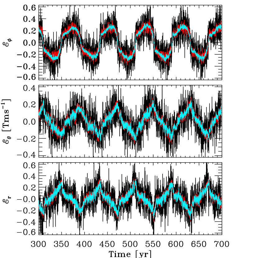
Figure 1: Time series of the turbulent electromagnetic force (black) extracted directly from EULAG-MHD simulation output (viz. eq. (3)) in the course of 5 complete magnetic cycles. The light blue time series show the emf reconstructed using the original procedure of Racine et al. (2011), i.e., fitting only the $\bm{\alpha}$-tensor, while the red time series are the emf components reconstructed from the expanded SVD procedure detailed below, in which both $\bm{\alpha}$ and $\bm{\beta}$ are fitted to the emf (see text).

3.1 The singular value decomposition procedure

The procedure employed here to extract the $\bm{a}$ and $\bm{b}$-tensor components is a generalization of the method originally introduced by Racine et al. (2011). The idea is to take the emf and the mean (zonally-averaged) magnetic field from the simulation output of EULAG-MHD and seek time-independent numerical coefficients, specifically the components of $\bm{\widetilde{a}}$ and $\bm{\widetilde{b}}$, which provide the best possible match to eq. (8). This defines an optimization problem, which is tackled as a least-squares minimisation using Singular Value Decomposition (see Press et al. 1992, Section 15.4).

For a given component $m=(r,\theta,\phi)$ of the emf at a specific node of the computational grid $(r_{b},\theta_{c})$, we first define the time-dependent functions $\mathrm{y}(t)$ and $X(t)$:

$$\mathrm{y}(t)=\mathcal{E}_{m}(t,r_{b},\theta_{c})~{},$$ (13)

and

$$X(t)=[\langle B_{k}(t,r_{b},\theta_{c})\rangle,\,\partial_{r}\langle B_{k}(t,r_{b},\theta_{c})\rangle,\,\partial_{\theta}\langle B_{k}(t,r_{b},\theta_{c})\rangle]\,\,\,\textrm{for}\,\,\,k=r,\theta,\phi~{},$$ (14)

where for each time step of the simulation output, $X(t)$ at $(r_{b},\theta_{c})$ is a 9 components vector containing the mean magnetic field and its derivatives, as appearing on the RHS of eq. (8). We then define the vector $\bm{\varphi}$ at fixed $m$ as:

$$\varphi_{j}=[\widetilde{a}_{mk}(r_{b},\theta_{c}),\widetilde{b}_{mkr}(r_{b},\theta_{c}),\widetilde{b}_{mk\theta}(r_{b},\theta_{c})]~{},\,\,\,\textrm{for}\,\,\,k=r,\theta,\phi~{},$$ (15)

containing the value of $\bm{\widetilde{a}}$ for $j=1-3$ and $\bm{\widetilde{b}}$ for $j=4-9$ corresponding to a single component of the emf. In this notation, the parameterization of the emf is written as:

$$\mathrm{y}(t)=\sum\limits_{j=1}^{9}\varphi_{j}X_{j}(t)~{},$$ (16)

and the goal here is to find the 9 values of $\varphi_{j}$ that minimize the least-squares merit function:

$$\chi^{2}=\sum\limits_{i=1}^{N_{t}}\left[\mathrm{y}(t_{i})-\sum\limits_{j=1}^{9}\varphi_{j}X_{j}(t_{i})\right]^{2}~{},$$ (17)

where $N_{t}$ is the number of time-steps $t_{i}$. The design matrix A used in singular value decomposition procedure is constructed as $\mathrm{A}_{ij}=X_{j}(t_{i})$. In the present context this $N_{t}\times 9$ matrix depends on the large scale magnetic field and its spatial derivatives in $r$ and $\theta$, as per eq. (8). It can be decomposed as:

$$\mathbf{A}=\mathbf{U\cdot w\cdot V^{T}}~{},$$ (18)

where $\mathbf{U}$ is an $N_{t}\times 9$ orthogonal matrix, $\mathbf{w}$ is a $9\times 9$ diagonal matrix containing the so-called singular values, and $\mathbf{V}$ is a $9\times 9$ orthogonal matrix. The solution of $\bm{\varphi}$ is then given by;

$$\bm{\varphi}=\mathbf{V\cdot w^{-1}\cdot U^{T}\cdot y}~{},$$ (19)

which is where the emf finally enters the problem, though the $\mathrm{y}=(\mathrm{y}_{1},\mathrm{y}_{2},...\mathrm{y}_{N_{t}})$ time series.

This whole procedure is repeated three times for $m=r,\theta$ and $\phi$ and at all grid points in the meridional plane so as to construct the spatial profiles of all 9 components of the $\bm{\widetilde{a}}$ pseudotensor, and of the 18 components of the $\bm{\widetilde{b}}$ pseudotensor accessible in a system axisymmetric on the large scales.

A great practical advantage of the SVD decomposition is that it also returns the standard deviation ($\sigma$) via:

$$\sigma^{2}_{j}=\sum\limits_{i=1}^{9}\left(\frac{\mathrm{V}_{ji}}{\mathrm{w}_{ii}}\right)^{2}~{}.$$ (20)

For each component of $\bm{\alpha}$ and $\bm{\beta}$ computed, we can thus recover an error estimate. In all results presented in what follows, a measurement of a tensor component is deemed significant if it deviates from zero by more than its associated standard deviation. Note that $\sigma$ is a function of $\mathrm{\mathbf{V}}$ and $\mathrm{\mathbf{w}}$, both originating from the decomposition of the design matrix, which therefore implies that $\sigma$ is set by fluctuations of the mean magnetic field and its derivatives, but not by fluctuations of the emf components. Typically, the inclusion of the $\bm{\beta}$-tensor in the SVD procedure tends to increase the standard deviation with respect to reconstruction fitting only the $\bm{\alpha}$-tensor, as in Racine et al. (2011), because the time series of mean field spatial derivatives tend to be noisier than those of the mean field components.

3.2 Results for the $\boldmath{\alpha}$-tensor

Racine et al. (2011) extracted the $\bm{\alpha}$-tensor from the output of an earlier EULAG-MHD simulation of much shorter duration, retaining only the first term in the emf development given by eq. (4). Including now the second term, proportional to first derivatives of the mean field not only introduces additional explicit contributions to the $\bm{\alpha}$-tensor components (see eqs. (9a)–(9f)), but also alters the fit altogether. In either cases the reconstructed emf offers a very good representation of the emf measured directly from the simulation output via eq. (3) herein, as shown by the red and blue time series superimposed on the measured emf on Figure 1. However, as we shall see presently, including the $\bm{\beta}$-tensor does reduce the rms residual with respect to the measured emf.

It will prove interesting to first quantify the differences between the $\bm{\alpha}$-tensors, extracted with and without the $\bm{\beta}$-terms so as to reassess the reliability and accuracy of the Racine et al. (2011) $\bm{\alpha}$-tensor extraction. Such a comparison is presented on Figure 2, for two of the diagonal components of the $\bm{\alpha}$-tensor (two leftmost columns) and two components of the turbulent pumping speed (two rightmost columns, viz. eq. (6)). The top row shows results where only the $\bm{a}$ term is retained in eq. (4), while in the bottom row both ${\bm{a}}$ and ${\bm{b}}$ are used in the SVD fitting procedure, as described in §3.1. A white mask is applied to show only regions of the meridional plane where the measured tensor components deviate from zero by more than one standard deviation. Both sets of tensor component are morphologically quite similar, the primary difference being a small reduction in overall magnitude when the ${\bm{b}}$ term is retained in the analysis, ranging from $\simeq 15$% for $\gamma_{r}$, up to $50$% for $\alpha_{\phi\phi}$, this latter, larger difference being dominated by variations in the polar regions.

Figure 3 shows radial cuts for four $\bm{\alpha}$-tensor components extracted at different latitudes with and without the inclusion of the $\bm{\beta}$-tensor. The sets of cuts usually stand within each other’s one-$\sigma$ standard deviation returned by the SVD fit, the most significant difference being found with the $\alpha_{\phi\phi}$ component, which stand between 1 and $\simeq 2\sigma$ of each other at high latitudes (viz. Fig. 3A).

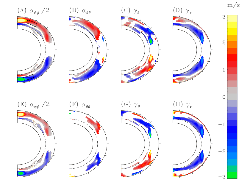
Figure 2: Illustration of the $\alpha_{\phi\phi}$ (leftmost column) and $\alpha_{\theta\theta}$ (second column) components, together with the turbulent pumping components $\gamma_{\theta}$ (third column) and $\gamma_{r}$ (rightmost column) as extracted from the 1600 yr long EULAG-MHD millenium simulation. The top row shows results when only the first term is retained on the RHS of eq. (4), while the bottom row shows the corresponding results when the first two terms are retained. A white mask is applied in regions of the meridional plane where the signals is lower than one standard deviation. On each panels, the dash-line indicates the base of the convectively unstable fluid layer, and the tickmarks on the outer boundary of each diagram are drawn at intervals of $20^{\mathrm{o}}$. The box drawn in panel (A) shows the integration domain used in the $\alpha$-quenching analysis of §4.1 below.

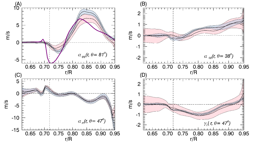
Figure 3: Radial cuts of four selected $\bm{\alpha}$-tensor components taken at different latitudes without (blue) and with (pink) the inclusion of $\bm{\beta}$ in the SVD fitting procedure. The colored area indicate the correponding 1$\,\sigma$ region of significance, and the vertical dashed line the location of the core-envelope interface. Panel (A) also includes (in blue) a radial profile of the SOCA $\alpha*$ (eq. (21)) extracted at the same latitude and divided by a factor 4.5 (see text).

3.3 Results for the $\boldmath{\beta}$-tensor

Figure 4 shows the nine $\bm{\beta}$-tensor components reconstructed via eqs. (15d)—(15e) in Schrinner et al. (2007) from the $\bm{\widetilde{b}}$ components extracted using our SVD least-squares minimization method. Once again a white mask is used to show only the regions of the meridional plane where the tensor components exceed the one standard deviation level, as returned by the SVD procedure. As self-consistency check, we also applied a modified form of the SVD procedure, retaining only the $\bm{\widetilde{b}}$ coefficients, to the residual $\bm{\mathcal{E}}-\bm{\alpha}\langle{\bm{B}}\rangle$ of a SVD extraction carried out only with the $\bm{\widetilde{a}}$ terms, as in Racine et al. (2011). The resulting $\bm{\beta}$-tensor closely resembles its counterpart returned by the complete extraction procedure described in § 3.1 (viz. Fig. 4).

The tensor is noisier, and typically shows smaller significance regions than the $\bm{\alpha}$-tensor. Note however that the diagonal elements are positive definite almost everywhere, which offers some confidence that the results are physically meaningful. Moreover, the overall amplitudes are in the range $10^{7}$—$10^{8}\,\mathrm{m}^{2}/\mathrm{s}$, which is consistent with other estimates of dissipation in similar EULAG simulations (see, e.g., Strugarek et al., this volume). The largest amplitude, peaking at $\simeq 10^{8}\,\mathrm{m}^{2}/\mathrm{s}$, are obtained for the $\beta_{\phi\phi}$ component, with most of the domain returning a signal well above our one standard deviation mask. This component thus dominates the diagonal, and will be used preferentially in what follows when comparing to SOCA reconstructions and measuring magnetically-mediated quenching.

While many $\bm{\beta}$-tensor components lie below the 1$\sigma$ threshold in extended portions of the meridional place, the rms residual between the emf (Fig. 5A) and the reconstructed emf (Fig. 5B) is reduced after the inclusion of the $\bm{\beta}$-tensor in the SVD procedure. This residual is plotted in Fig. 5D together with the residual for a SVD fit using only the $\bm{\alpha}$-tensor (Fig. 5C). Comparison of those two panels reveals a slight decrease of the residual when $\bm{\beta}$ is included in the SVD procedure of the emf: averaged over the meridional plane, the residual drops from $0.046$ (Fig. 5C) to $0.043\,\mathrm{Tm}/\mathrm{s}$ (Fig. 5D), amounting to a 6.5$\%$ decrease. This indicates that the slightly higher level of fluctuations observed in the red time series on Fig. 1 does no result from a noisier reconstruction, but rather from the fitting procedure capturing more of the physical variability present in the extracted emf components.

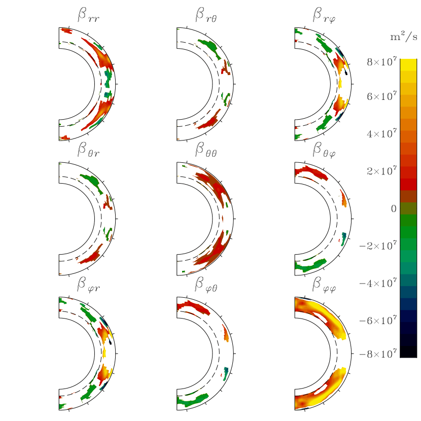
Figure 4: Reconstruction of the $\bm{\beta}$-tensor from the 18 accessible components of the pseudo-tensor $\bm{\widetilde{b}}$ extracted from the EULAG-MHD millenium simulation. The format is similar to Fig. 2, with the dashed line indicating the base of the convectively unstable fluid layers. A white mask applied to regions of the meridional plane where the tensor components fall below the one-standard deviation level.

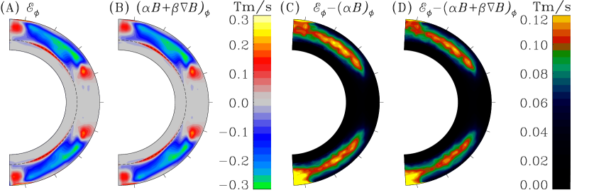
Figure 5: Mean azimutal turbulent electromotive force in a meridional plane for the concatenated set of cycle maximum 14 month-wide block as computed via eq. (3) in panel (A) and as reconstructed via eq. (8) in panel (B). Rms residuals averaged over the same concatenated set for the reconstructed emf where in the first (panel (C)) or both (panel (D)) term are retained in the SVD procedure.

3.4 Comparison with SOCA

In the case of isotropic, homogeneous turbulence, the $\bm{\alpha}$ and $\bm{\beta}$-tensors simplify to $\alpha_{ij}=\alpha\delta_{ij}$ and $\beta_{ij}=\beta\epsilon_{ijk}$. The scalar coefficients $\alpha$ and $\beta$ can be computed under the Second Order Correlation Approximation (SOCA) as:

$$\alpha*=-\frac{\tau_{c}}{3}\langle\bm{u}^{\prime}\cdot\nabla\times\bm{u}^{\prime}\rangle~{},$$ (21)

and

$$\beta*=\frac{\tau_{c}}{3}\langle(\bm{u}^{\prime})^{2}\rangle~{},$$ (22)

where $\tau_{c}$ is the coherence time of the turbulence, and the terms in the averaging brackets on the RHSs are, respectively, the mean kinetic helicity and the turbulent intensity of the small-scale flow component (see, e.g., Ossendrijver 2003; Schrijver & Siscoe 2009). Figure 6A and D show the corresponding $\alpha$ and $\beta$ coefficients, assuming a coherence time equal to the turnover time of the convective flow; the latter is estimated as $H_{\rho}/u^{\prime}$, where $H_{\rho}$ is the density scale height and $u^{\prime}$ is the rms small-scale flow speed.

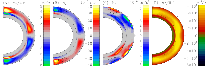
Figure 6: SOCA-based reconstructions of the isotropic part of the $\bm{\alpha}$-tensor (in A) from the kinetic helicity (in B) as given by eq. (21); compare with Fig. 2A and E. Panel C illustrate the current helicity as computed by the second term on the RHS of equation (26), note the different ranges of the color scales in (B) and (C). Panel D shows the corresponding reconstruction for the isotropic part of the $\bm{\beta}$-tensor via eq. (22); compare with $\beta_{\phi\phi}$ at bottom right in Fig. 4. The dashed line indicates the base of the convectively unstable fluid layers and the boxes drawn in panels (B) and (C) shows again the integration domain used in the following $\alpha$-quenching analysis of §4.1.

The resemblance with the actual $\alpha_{\phi\phi}$, as extracted from the simulation via the SVD least-squares method in Fig. 2E and Fig. 3A, is quite good: both tensor components peak at polar latitudes, show a secondary maximum at low latitude, and undergo a sign change just above the core-envelope interface. The main discrepancy resides in the absolute magnitudes, with $\alpha*$ being larger than $\alpha_{\phi\phi}$ in its region of significance by an average factor of $\simeq 4.5$.

Figure 6D shows the corresponding SOCA coefficient $\beta*$ computed via eq. (22), which is best compared to the $\beta_{\phi\phi}$ component in the lower right of Fig. 4. Here also the general spatial variations of the two quantities are similar, the main difference being one of overall amplitude, with the SOCA expression exceeding the extracted $\beta_{\phi\phi}$ by an average factor of $\simeq 5.5$ over its region of significance. That we recover a scaling factor almost identical to that characterizing the ratio of $\alpha*$ to $\alpha_{\phi\phi}$ suggests that the discrepancy may lie with our choice of correlation time $\tau_{c}$ in eqs. (21)—(22), indicating in turn that equating $\tau_{c}$ to the convective turnover time may be a large overestimate. Interestingly, a short correlation time is one of the physical regimes under which the SOCA approximation can be expected to hold (Ossendrijver 2003).

4 Magnetic quenching of the turbulent emf

In the nonlinearly saturated regime of dynamo action, one would expect the Lorentz force associated with the magnetic field to impact the inductive flows, including at the turbulent scales. Starting with the pioneering study of Pouquet et al. (1976), this magnetic quenching of the emf has by now been measured in a variety of MHD turbulence simulations. Karak et al. (2014) §1 give a good survey of these various quenching measurements. In most cases what is being measured is the suppression of the emf in response to the application of an external large-scale magnetic field. This is also the case for the rotating convection simulations for which Karak et al. (2014) report quenching results: quenching is measured with respect to the strength of imposed large-scale “test-fields”. One important exception is the analyses of Brandenburg et al. (2008), who investigated quenching of the $\alpha$-effect and turbulent diffusivity, both in full tensorial form, in a cartesian box MHD simulation of helically forced turbulence autonomously generating a large-scale magnetic component. The EULAG-MHD millenium simulation introduced above also generates autonomously its own large-scale magnetic field, and so offers the possibility to measure directly the quenching of the emf, without the artificial introduction of external large-scale field components.

4.1 $\alpha$ Quenching

We first repeat the SVD fitting procedure used to obtain the $\alpha_{\phi\phi}$ tensor component plotted on Fig. 2A, this time over disjoint 100-month wide temporal blocks (about one fifth of the half-cycle duration) centered on epochs of cycle maxima and minima, the latter determined on the basis of the time series of magnetic energy associated with the large-scale magnetic component waxing and waning in the course of the simulation. We opted to integrate the $\alpha_{\phi\phi}$ component over the domain indicated on Figure 2A. This selected area is one where $\alpha_{\phi\phi}$ does not change sign, has a magnitude much larger than its standard deviation, and is located at high latitude, where the large-scale dipole moment is building up (see Fig. 1B in Passos & Charbonneau 2014). Henceforth, unless explicitly stated otherwise, spatial averaging is always carried out over this domain, separately for each hemisphere. The results are shown on Fig. 7, in the form of bar charts, one bar per temporal block, color-coded to indicate min/max cycle phase. The error bars assigned to each measurement are obtained by integrating the standard deviation over the same spatial domain as $\alpha_{\phi\phi}$, assuming that fluctuations at each grid point are uncorrelated. With only a few exceptions, the $\alpha_{\phi\phi}$ component extracted from each of the 34 cycles in the simulation show a statistically significant difference between epochs of maxima and minima. Qualitatively similar results are obtained for the other components of the $\bm{\alpha}$-tensor.

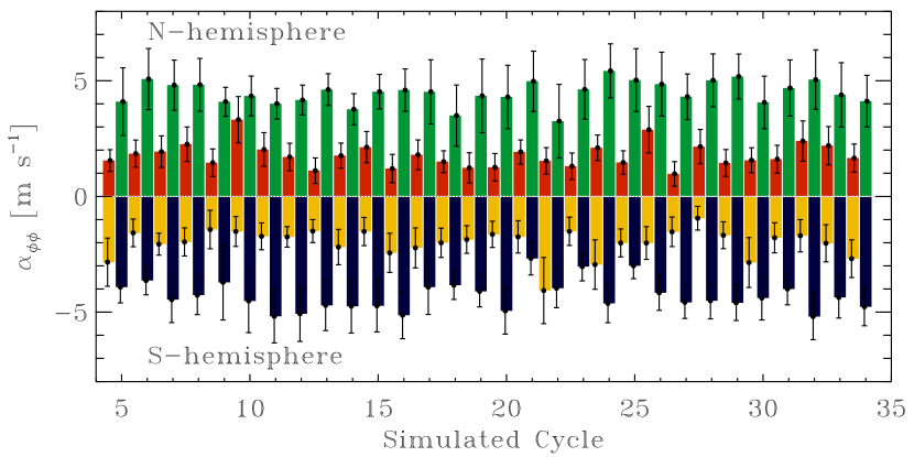
Figure 7: Bar diagram showing the magnitude of the $\alpha_{\phi\phi}$ tensor component, averaged over the domain shown on Fig. 2A. The top (bottom) half of the diagram correspond to the Northern (Southern) hemisphere. The SVD fitting procedure was applied here over 100-month wide segments centered over successive cycle maxima (red and yellow) or minima (green and black). Error bars are estimated by averaging the standard deviation over the same domain, assuming spatially uncorrelated statistics. With only a few exceptions, cycle maxima show a level of $\alpha$-quenching significantly exceeding the error bars.

Figure 8 shows, in meridional planes, the spatial profile of the $\alpha_{\phi\phi}$ tensor component for the concatenated set of cycle minimum 100 month-wide blocks in (A), cycle maximum blocks in (B), and the full simulation in (C), for comparison purposes. In all cases white contours delineate the 1$\,\sigma$ significance regions, as returned from the SVD algorithm. Comparing panels (A) and (B) reveals that quenching of this tensor component involves an overall reduction of its amplitude, leaving its spatial profile largely invariant. The $\alpha_{\theta\theta}$ tensor component behaves similarly in this respect.

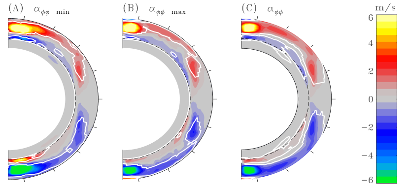
Figure 8: The $\alpha_{\phi\phi}$ in the meridional plane, extracted from (A) the concatenation of all “minimum” blocks on Fig. 7, (B) the “maximum” blocks, and the full simulation in (C). White contours delineate the regions of significance ($1\,\sigma$).

Next, we carry out a similar exercise, this time extracting the $\bm{\alpha}$-tensor over successive 100-month long temporal block, extending over the whole simulation with a 50% overlap from block to block. For each such block we average the $\alpha_{\phi\phi}$ component and the magnetic energy over the same spatial domain as previously described. The $\alpha_{\phi\phi}$ component shows a clear decrease with magnetic energy, dropping from a mean value $\simeq 4.4\,$m s^-1 at cycle minima, down to $1.8\,$m s^-1 at cycle maxima, amounting to a reduction by a substantial factor of three. Similar levels of quenching are observed with other $\bm{\alpha}$-tensor components, e.g., the averaged $\alpha_{r\theta}$ drops from $1.5$ to $0.7\,$m s^-1 from cycle minimum to maximum.

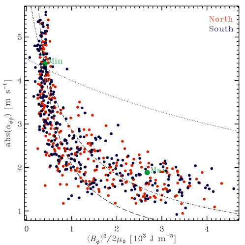
Figure 9: Variation of the $\alpha_{\phi\phi}$ component versus magnetic energy of the zonal magnetic component, both again averaged over the domain shown on Fig. 2A. The SVD fit is carried out over successive 100-month wide time blocks, with 50% overlap between successive blocks, and the magnetic energy is averaged similarly in space and time. The larger green solid dots indicate the mean values for these quantities at cycle maxima and minima, taken directly from Fig. 7. $\alpha$-quenching is again quite obvious here, with $\alpha_{\phi\phi}$ decreasing by a factor of $\sim 3$ over the range of magnetic energy density sampled throughout the cycles. The dotted curve shows the variation expected from the standard algebraic quenching formula (eq. (24)), and the dash-dotted and dashed curves result from the alternate strong quenching expression (viz. eq. (25)), with $R_{m}=10$ and $50$ respectively.

An $\alpha$-quenching parametric formulae commonly used in mean-field dynamo models is based on the assumption that the $\alpha$-effect becomes suppressed once turbulent fluid motions reach energy equipartition with the large-scale magnetic field, i.e.,

$${1\over 2}\rho(u_{\rm rms}^{\prime})^{2}={\langle{\bm{B}}\rangle^{2}\over 2\mu_{0}}~{},$$ (23)

where $\mu_{0}$ is the permeability of free space and $\rho$ is the density of the plasma. The field strength at which this equality is satisfied defines the equipartition field strength (hereafter denoted $B_{\rm eq}$). Note that here the small-scale flow $u_{\rm rms}^{\prime}$ is extracted from the simulation output of EULAG-MHD, and therefore is distinct from the small-scale flow that would characterize a purely hydrodynamical simulation operating in the same parameter regime. Such hydrodynamical flows are typically used as baseline in many quenching analyses using externally-imposed magnetic fields (see e.g., Karak et al. 2014).

The working hypothesis embodied in eq. (23) is most often introduced in mean-field models by adding an explicit algebraic dependence on $\langle{\bm{B}}\rangle$ to the $\bm{\alpha}$-tensor components:

$$\alpha\to{\alpha_{0}\over 1+(\langle{\bm{B}}\rangle^{2}/B_{\rm eq}^{2})}~{},$$ (24)

where $\alpha_{0}$ is the magnitude of the $\bm{\alpha}$-tensor in the absence of large-scale magnetic field. This ad hoc expression obviously “does the right thing”, in that it ensures $\alpha\to 0$ as $\langle{\bm{B}}\rangle\gg B_{\rm eq}$. However, attempts to validate such expression against MHD numerical simulations of forced helical flows have instead lead to the alternate “strong quenching” expression (Vainshtein & Cattaneo 1992):

$$\alpha\to{\alpha_{0}\over 1+R_{m}(\langle{\bm{B}}\rangle^{2}/B_{\rm eq}^{2})}~{},$$ (25)

where $R_{m}$ is the magnetic Reynolds number characterizing the flow. With $R_{m}\sim 10^{8}$–$10^{10}$ in the solar convection zone, $\alpha$-quenching then sets in at a magnitude of $\langle{\bm{B}}\rangle$ four to five orders of magnitude below equipartition. The difference between eqs. (24) and (25) hinges on the fact that at high-$R_{m}$, the turbulent flow first reaches energy equipartition with ${\bm{B}}^{\prime}$, not $\langle{\bm{B}}\rangle$; eq. (25) then follows from the scaling ratio ${\bm{B}}^{\prime}/\langle{\bm{B}}\rangle\sim\sqrt{R_{m}}$, expected in the limit $R_{m}\gg 1$ (see Cattaneo & Hughes 1996; Hubbard & Brandenburg 2012). This catastrophic quenching is believed to reflect a cascade of magnetic helicity to small scales, required under the constraint of total magnetic helicity conservation (Brandenburg 2001; Field & Blackman 2002). It can be alleviated by allowing a flux of helicity through the simulation boundaries (see, e.g., Käpylä et al. (2008) and discussion therein).

In the simulation analyzed in this paper $\rho=42\,$kg m^-3 and $u_{\rm rms}^{\prime}\simeq 20\,$m s^-1 in the middle of averaging domain used for the $\alpha$-quenching analysis, which leads to a kinetic energy density $e_{k}\simeq 8000\,$J m^-3, corresponding to an equipartition field strength of $\simeq 0.15\,$T, in good agreement with the energy density of the small-scale magnetic component averaged over the same subdomain. Fig. 9 indicates that quenching is already well underway at $\langle{B_{\phi}}\rangle^{2}/2\mu_{0}\simeq 10^{3}\,$J m^-3. This suggests that $\alpha$-quenching in our simulation is mediated primarily by the small-scale magnetic field, even though the magnetic Reynolds number characterizing this simulation is only a few tens.

Attempts to fit the classical quenching expression given by eq. (24) to the simulation data presented in Figure 9 yield an extremely poor fit (dotted line), due to the strong concavity of the observed trend. Similar attempts using the strong quenching expression (25) fare definitely better, although no single combination of $\alpha_{0}$ and $R_{m}$ fits the simulation data well over its full range. The dash-dotted and dashed curves on Fig. 9 show the quenching predicted by eq. (25) for $R_{m}=10$ and $R_{m}=50$, respectively, with $\alpha_{0}$ adjusted to fit approximately the mean $\alpha_{\phi\phi}$ value at cycle minima. The rapid initial drop of $\alpha_{\phi\phi}$ is best reproduced by picking a higher $R_{m}$, but the flat, extended tail is better fit with a lower $R_{m}$. Note that a magnetic Reynolds number of a few tens is actually consistent with other estimates obtained for this simulation by different means, e.g. from the turbulent spectrum, and thus presents a form of internal consistency with the strong quenching interpretation.

Whether in their weak or strong form, the algebraic quenching expressions (24) and (25) remain extreme simplifications of the complexity of turbulent flow-field interactions. The numerical simulations of Pouquet et al. (1976) suggest that for MHD turbulence with short coherence time, eq. (21) should be replaced by:

$$\alpha*=-{\tau_{c}\over 3}(\langle{{\bm{u}}^{\prime}\cdot\nabla\times{\bm{u}}^{\prime}}\rangle-\rho^{-1}\langle{{\bm{j}}^{\prime}\cdot{\bm{B}}^{\prime}}\rangle)~{}.$$ (26)

The first term in parentheses on the RHS of this expression is again the kinetic helicity $h_{v}$, and the second is its magnetic equivalent, namely the current helicity, where $\mu_{0}{\bm{j}}^{\prime}=\nabla\times{\bm{B}}^{\prime}$, a quantity closely related to the usual magnetic helicity. Note that this magnetic contribution to the $\alpha$-effect has a sign opposite to that of the kinetic contribution, and reflects the small-scale magnetic helicity will tend to counteract the kinetic helicity of the small-scale flow, a general property of flow-field interactions in the MHD limit.

We can take advantage of the fact that eq. (26) offers a good representation of the $\alpha_{\phi\phi}$ component extracted from the simulation (viz. Fig. 2) to investigate the physical origin of the $\alpha$-quenching measured in the simulation. The formulation known as dynamical $\alpha$-quenching assumes that reduction of the $\alpha$-effect takes place through the growth of the magnetic term on the RHS of eq. (26). This growth is seen as an unavoidable consequence of magnetic helicity conservation, which requires accumulation of magnetic helicity of one sign at small scales, if a large-scale magnetic component with helicity of opposite sign is to be produced by turbulent dynamo action (Brandenburg 2001).

Figure 10 shows the temporal variations of the kinetic helicity $h_{v}$ and magnetic helicity $h_{b}$ over the course of the 34 cycles in the simulation, in the form of a trajectory in the 2D phase space $[h_{v},h_{b}]$. Both helicities are averaged over the high latitude domain depicted on Fig. 6B and C, as well as in time, over 100-month wide temporal blocks overlapping by 50%, as on Figure 9. The plot shows the trajectory associated with the Northern hemisphere, but the Southern hemisphere trajectory is similar, except for being reflected about the origin. One full magnetic cycle corresponds here to two clockwise circuits along the loop-like path, and the solid green dots show the locii corresponding to the averages of maxima and minima on Fig. 7.

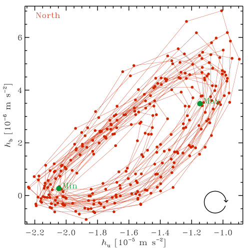
Figure 10: Phase space portrait of the joint variations of the kinetic and current helicities in the Northern hemisphere. As in previous Figures, $h_{v}$ and $h_{b}$ are averaged over the domain shown on Fig. 6B and C and averaged over successive 100-month wide temporal blocks with 50% overlap (solid dots), with consecutive blocks connected by a line segment. The trajectory runs clockwise on this plot, with mean values over cycle maxima and minima indicated by solid green dots.

The cyclic growth of the current helicity $h_{b}$ from cycle minimum to subsequent maximum, followed by a decrease to the next minimum, actually contributes an increase of the $\alpha$-effect in the integration domain considered here (box on Fig. 6C). This happens because in this region, the current helicity has a sign opposite to the kinetic helicity, unlike in most other regions of the domain, where the opposite situation prevails and the current helicity opposes the kinetic helicity, as per eq. (26). This latter behavior is generally consistent with the picture of dynamical $\alpha$-quenching, according to which the cascade of magnetic helicity to small-scale during the growth phase of the cycle eventually leads to a saturation of the large-scale dynamo. Nonetheless, here the increase of $\alpha$ mediated by the growing current helicity is erased by a far more substantial variation of the kinetic helicity, which drops by almost a factor of two between minima and maxima. Repeating the same analysis with the integration region moved to lower latitude yields different patterns, but in all cases the kinetic helicity shows a reduction by factors in the range $\simeq 1.5$–2 between the minimum and maximum phases of the magnetic cycle.

In view of the relative magnitudes of $h_{v}$ and $h_{b}$ (cf. Fig. 6B and C), if eq. (26) is taken at face value then one would conclude that the cyclic variations of kinetic helicity dominates variations of current helicity in quenching the $\alpha$-effect at most locations in our simulation domain. This is a different pattern of quenching than measured by Brandenburg et al. (2008) in their helically forced simulation, in which the kinetic helicity remained essentially constant and the reduction of the $\alpha$-effect could be traced to a corresponding increase of the current helicity. The difference is perhaps not surprising, since their simulation is helically forced whereas in our case the forcing is thermal and helicity is introduced through the action of the Coriolis force.

The EULAG-MHD “millenium” simulation providing the numerical data used for all analyses presented in this paper achieves stability through implicit diffusivities associated with the numerical advection scheme, which here is the same for the advection of fluid velocity and magnetic field; in other words, here the magnetic Prandtl number is expected to be of order unity. The rather complex variation of kinetic versus current helicity is therefore unexpected, and must originate not with the dissipative properties of the simulation, but rather with changes in the character of the small-scale flows, presumably mediated by the large-scale magnetic field and perhaps also time-varying large-scale flows.

4.2 Diffusivity quenching

Measurements of the quenching of turbulent diffusivity in MHD simulations received comparatively less attention than $\alpha$-quenching. Section 1 of Karak et al. (2014) provides again a good survey of these measurements. Parametric diffusivity quenching, often akin to eq. (24) herein, have been incorporated into some mean-field dynamo models (e.g., Rüdiger et al. 1994), with goals as diverse as producing interface dynamos (Tobias 1996), achieving strong amplification to toroidal magnetic fields in the tachocline (Gilman & Rempel 2005), effecting the transition from diffusion-dominated to advection-dominated regimes in flux transport dynamos (Guerrero et al. 2009), or producing a strong radial diffusivity gradient in the outer convective envelope (Muñoz-Jaramillo et al. 2011).

In view of the $\bm{\beta}$-tensor measurements displayed on Fig. 4, we focus here only on the $\beta_{\phi\phi}$ component, for which a statistically significant determination is obtained over $70\%$ of the meridional plane. Following the same strategy just used for measuring $\alpha$-quenching, we segment the simulation output into two sets of disjoint 100-month wide blocks centered respectively on magnetic energy minima and maxima. We then repeat the SVD least-squares fit on the concatenation of each of these two sets of segments. In this manner we generate two “average” $\beta_{\phi\phi}$ components, respectively characterizing epochs of maxima or minima of the magnetic cycle. The result of this procedure is shown on panels A and B of Fig. 11, with panel (C) replicating the $\beta_{\phi\phi}$ extracted from the full simulation run. In all three panels the white contours marks the 1$\,\sigma$ region of significance as returned by the SDV procedure. As expected, the corresponding level of noise for $\beta_{\phi\phi}$ in epochs of minima and maxima are higher due to the reduced length of the simulation data.

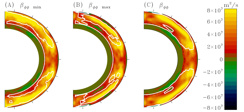
Figure 11: The $\beta_{\phi\phi}$ component extracted from the sets of disjoint 100-month wide temporal segments centered either on (A) minima or (B) maxima of the large-scale magnetic cycle. For comparison, panel (C) shows the corresponding plot for the whole simulation output, replicated from Fig. 4. The white contour marks the level where $\beta_{\phi\phi}$ is equal to the standard deviation returned by the SVD fitting procedure.

Evidently, the overall amplitude of $\beta_{\phi\phi}$ is reduced at times of cycle maxima, as compared to epochs of cycle minima. To quantify this level of reduction we average $\beta_{\phi\phi}$ within the statistically significant region located within the 1$\,\sigma$ contour, leading to values $6.0\times 10^{7}\,$m${}^{2}\,$s^-1 for minima, and $4.4\times 10^{7}\,$m${}^{2}\,$s^-1 for maxima, a $\simeq 36$% reduction. In comparison, the same average carried out for the $\beta_{\phi\phi}$ extracted over the full simulation yields $5.0\times 10^{7}\,\mathrm{m}^{2}/\mathrm{s}$. The Min-to-Max ratio is thus $\simeq 1.36$, much smaller than the reduction by a factor of $\sim 3$ determined for the components of the $\bm{\alpha}$-tensor (see Fig. 9). This is qualitatively consistent with other determinations of $\alpha$- and $\beta$-quenching in various types of 3D turbulent MHD simulations (see Karak et al. (2014), §1, and references therein).

5 Discussion and conclusion

We presented in this paper a reconstruction of the $\bm{\alpha}$ and $\bm{\beta}$-tensor characterizing the mean turbulent electromotive force operating in a EULAG-MHD global simulation of thermally-driven convection, specifically the “millenium simulation” presented in Passos & Charbonneau (2014). We generalized the original singular value decomposition-based least-squares minimization procedure of Racine et al. (2011), which was restricted to the $\bm{\alpha}$- tensor, to include also the simultaneous reconstruction of the $\bm{\beta}$-tensor.

Including the $\bm{\beta}$-tensor in the extraction procedure yields results for the $\bm{\alpha}$-tensor that are quite similar to the earlier extractions of Racine et al. (2011), who truncated the emf development eq. (4) already at the first term. The primary difference is in the amplitude of the $\bm{\alpha}$-tensor components, which tend to be smaller with the $\bm{\beta}$-tensor included. Interestingly, Augustson et al. (2015) report a similar level of variation when using their implementation of the SVD least-squares extraction scheme on their ASH simultion results, with the $\bm{\beta}$-tensor included or not in the extraction process. Indeed, for the bulk of the convecting layers the $\bm{\alpha}$-tensor extracted from Augustson et al. (2015)’s ASH simulation is quite similar to that characterizing our EULAG-MHD simulations (cf. Fig. 9 in Racine et al. 2011 to Fig. 13 in Augustson et al. 2015), keeping in mind that our $\theta$ is latitude, which leads to a sign difference for $\alpha_{(r\theta)}$, $\alpha_{(\theta\phi)}$, and $\gamma_{\theta}$). This was not necessarily to be expected, considering that the two simulations show some significant design differences, notably the presence of stably stratified fluid layer underlying the convecting layer in EULAG-MHD, distinct boundary conditions, very different numerical and temporal resolutions and, more importantly, different numerical diffusivities implicitly introduced at the smallest scales.

In a recent submission to ArXiv, Warnecke et al. (2016) apply their preferred test-field method, as well as a least-squares-based method analogous to that used in the present paper, to extract the $\bm{\alpha}$-tensors from the output of a spherical wedge MHD simulations of solar convection. Even though no error bars are provided for either method, the authors claim that these yield conflicting results (as per their Fig. 16), and on this basis conclude that the least-square-based method is “unreliable” (p 15) and “incorrect” (p 16). This conclusion stems from an additional a priori assumption being made, namely that the test-field results are by definition correct. Even if that were the case, comparisons of this nature require quantitative error estimates (cf. their Fig. 16 to Fig. 3 herein), to assess whether the differences measured are statistically significant to begin with.

The $\bm{\beta}$-tensor we extract from our EULAG-MHD millenium simulation is quite noisy, with limited regions of 1$\,\sigma$ significance. Nonetheless, the diagonal is clearly positive definite, with values $\sim 10^{7}$—$10^{8}\,$m${}^{2}\,$s^-1, commensurate with dissipation coefficient for similar EULAG simulations estimated by other means (see Strugarek et al., this volume), as well as with values typically used in mean-field dynamo models.

Our analysis of $\alpha$-quenching yields results in general qualitative agreement with the so-called strong quenching formulation, in which it is the small-scale magnetic field that first reaches equipartition with turbulent fluid motions and quenches the turbulent $\alpha$-effect. Note however that the magnetic Reynolds number characterizing our MHD simulation is relatively low, of the order of a few tens, with the consequence that energy density of the small-scale magnetic components exceeds that of the large-scale field by less than a factor of ten in the region of the simulation domain used for this quenching calculation. Although cyclic variations of the small-scale current helicity are measured in the simulation, the greater part of the $\alpha$-quenching appears to result from a reduction of the turbulent kinetic helicity. Approximately half of this decrease is due to a drop in the rms turbulent flow speed, while the other half results from a decrease in the alignment of the small-scale flow with respect to it vorticity vector. These results indicate that, at least in this simulation, quenching of the $\alpha$-effect is a fully magnetohydrodynamical phenomenon, finding its roots in magnetically-mediated changes in the patterns of turbulent convection (on this latter point see also Cossette et al. (2016), submitted to ApJ).

Independently of the applicability (or lack thereof) of the SOCA expressions for the $\bm{\alpha}$-tensor, our analysis indicates that even in the minimum phase of the magnetic cycles our $\alpha$-effect shows a strong dependence on magnetic energy, indicating that significant magnetic quenching is acting already then. Our $\alpha$-effect evidently operates in a strongly nonlinear regime at all phases of the large-scale magnetic cycles unfolding in the simulations, as seems to also be the case in the simulations of Käpylä et al. (2012, 2013).

We also carried out measurements of diffusivity quenching, limited at this point in time to the $\beta_{\phi\phi}$ component. We find the turbulent diffusivity to suffer much less quenching than the $\alpha$-effect, specifically $\simeq 36\%$ versus a factor of $\simeq 3$ for $\alpha$$\alpha$$\alpha$$\alpha$. This much weaker magnetic quenching of the turbulent diffusivity is in qualitative agreement with the findings of Brandenburg et al. (2008), even though the simulation analyzed by these authors used a geometrical setup and turbulent forcing quite different from ours.

Under a strictly scriptural interpretation of mean-field electrodynamics, the $\bm{\alpha}$- and $\bm{\beta}$-tensors are fundamentally linear, hydrodynamical quantities which characterize the inductive properties of a flow unaffected by the presence of magnetic fields at any scale. Here, in contrast, we are fitting eq. (8) to numerical data taken from a MHD simulation having reached its nonlinearly saturated stage. The $\bm{\alpha}$- and $\bm{\beta}$-tensor extracted in this manner are thus not, a priori, the same physical objects. They must be interpreted as coefficients quantifying an empirical parametrization of the nonlinearly saturated turbulent electromotive force in terms of the large-scale magnetic field and its derivatives. That they do so in a meaningful manner is supported by the fact that upon being inserted in a conventional axisymmetric kinematic $\alpha^{2}\Omega$ mean-field model, they produce a large-scale magnetic field exhibiting a spatiotemporal evolution resembling reasonably well that observed in the original MHD simulation from which the tensors are extracted (see §3.2 in Simard et al. 2013).

More surprising is the fact that the isotropic parts of the $\bm{\alpha}$ and $\bm{\beta}$-tensors extracted from the simulation show fairly good agreement with their linear forms, as computed under the second order correlation approximation. The most prominent discrepancy, namely the overall amplitude of the (isotropic) SOCA $\alpha*$ and $\beta*$ being larger by a factor of about 5, may hold a clue as to why the general spatial form of the tensors are otherwise so similar. The SOCA estimates require the specification of the correlation time of the turbulence flow ($\tau_{c}$ in eqs. (21), (22) and (26)), a quantity notoriously difficult to extract from numerical simulations. As a first cut we simply followed Brown et al. (2010) and set $\tau_{c}$ equal to the mean turnover time $\tau_{u}$ of the small-scale flow, the latter estimated from the density scale height $H_{\rho}$ and rms turbulent flow speed $u^{\prime}_{\rm rms}$; in other words, we have assumed the Strouhal number ${\rm St}=\tau_{c}/\tau_{u}$ to be unity. Matching the amplitude of the SOCA coefficient to those of the tensors extracted from the simulation requires reducing the Strouhal number by a factor of $\simeq 5$, which then puts us in the regime ${\rm St}<1$, in which the SOCA approximation is actually expected to hold (Pouquet et al. 1976). We view this as an encouraging indication of internal consistency in our analysis and interpretation, notwithstanding the fact that the results presented here pertain to a single simulation carried out at relatively low Reynolds number, and that our turbulent diffusivity results remain at this writing limited in scope.

We wish to thank Antoine Strugarek for useful discussions, and two anonymous referees for some useful comments and suggestions. This work was supported by the Natural Sciences and Engineering Research Council of Canada, the Fond Québécois pour la Recherche – Nature et Technologie, the Canadian Foundation for Innovation, and time allocation on the computing infrastructures of Calcul Québec, a member of the Compute Canada consortium. CS is also supported in part through a graduate fellowship from FRQNT/Québec.

References

- Augustson et al. (2015) Augustson, K., Brun, A. S., Miesch, M., & Toomre, J. 2015, ApJ, 809, 149
- Beaudoin et al. (2013) Beaudoin, P., Charbonneau, P., Racine, E., & Smolarkiewicz, P. K. 2013, Sol. Phys., 282, 335
- Brandenburg (2001) Brandenburg, A. 2001, ApJ, 550, 824
- Brandenburg et al. (2008) Brandenburg, A., Rädler, K.-H., Rheinhardt, M., & Subramanian, K. 2008, ApJ, 687, L49
- Brandenburg & Sokoloff (2002) Brandenburg, A., & Sokoloff, D. 2002, Geophys. Astrophys. Fluid Dyn., 96, 319
- Brandenburg & Subramanian (2005) Brandenburg, A., & Subramanian, K. 2005, Phys. Rep., 417, 1
- Brown et al. (2010) Brown, B. P., Browning, M. K., Brun, A. S., Miesch, M. S., & Toomre, J. 2010, ApJ, 711, 424
- Brown et al. (2011) Brown, B. P., Miesch, M. S., Browning, M. K., Brun, A. S., & Toomre, J. 2011, ApJ, 731, 69
- Cattaneo & Hughes (1996) Cattaneo, F., & Hughes, D. W. 1996, Phys. Rev. E, 54, 4532
- Charbonneau (2010) Charbonneau, P. 2010, Liv. Rev. Sol. Phys., 7
- Charbonneau (2014) —. 2014, ARA&A, 52, 251
- Charbonneau & Smolarkiewicz (2013) Charbonneau, P., & Smolarkiewicz, P. K. 2013, Science, 340, 42
- Cossette et al. (2016) Cossette, J. F., Charbonneau, P., Smolarkiewic, P. K., & Rast, M. 2016, Submitted to ApJ
- Fan & Fang (2014) Fan, Y., & Fang, F. 2014, ApJ, 789, 35
- Field & Blackman (2002) Field, G. B., & Blackman, E. G. 2002, ApJ, 572, 685
- Ghizaru et al. (2010) Ghizaru, M., Charbonneau, P., & Smolarkiewicz, P. K. 2010, ApJ, 715, L133
- Gilman & Rempel (2005) Gilman, P. A., & Rempel, M. 2005, ApJ, 630, 615
- Guerrero et al. (2009) Guerrero, G., Dikpati, M., & de Gouveia Dal Pino, E. M. 2009, ApJ, 701, 725
- Hubbard & Brandenburg (2012) Hubbard, A., & Brandenburg, A. 2012, ApJ, 748, 51
- Käpylä et al. (2008) Käpylä, P. J., Korpi, M. J., & Brandenburg, A. 2008, A&A, 491, 353
- Käpylä et al. (2009) —. 2009, A&A, 500, 633
- Käpylä et al. (2010) Käpylä, P. J., Korpi, M. J., Brandenburg, A., Mitra, D., & Tavakol, R. 2010, Astronom. Nach., 331, 73
- Käpylä et al. (2012) Käpylä, P. J., Mantere, M. J., & Brandenburg, A. 2012, ApJ, 755, L22
- Käpylä et al. (2013) Käpylä, P. J., Mantere, M. J., Cole, E., Warnecke, J., & Brandenburg, A. 2013, ApJ, 778, 41
- Karak & Choudhuri (2011) Karak, B. B., & Choudhuri, A. R. 2011, MNRAS, 410, 1503
- Karak et al. (2014) Karak, B. B., Rheinhardt, M., Brandenburg, A., Käpylä, P. J., & Käpylä, M. J. 2014, ApJ, 795, 16
- Kitchatinov & Olemskoy (2012) Kitchatinov, L. L., & Olemskoy, S. V. 2012, Sol. Phys., 276, 3
- Krause & Rädler (1980) Krause, F., & Rädler, K.-H. 1980, Mean-field magnetohydrodynamics and dynamo theory (Oxford, Pergamon Press, Ltd.)
- Lawson et al. (2015) Lawson, N., Strugarek, A., & Charbonneau, P. 2015, ApJ, 813, 95
- Masada et al. (2013) Masada, Y., Yamada, K., & Kageyama, A. 2013, ApJ, 778, 11
- Miesch (2007) Miesch, M. S. 2007, ApJ, 658, L131
- Moffatt (1978) Moffatt, H. K. 1978, Magnetic field generation in electrically conducting fluids (Cambridge University Press, 1978. 353 p., Cambridge)
- Muñoz-Jaramillo et al. (2011) Muñoz-Jaramillo, A., Nandy, D., & Martens, P. C. H. 2011, ApJ, 727, L23
- Nelson et al. (2013) Nelson, N. J., Brown, B. P., Brun, A. S., Miesch, M. S., & Toomre, J. 2013, ApJ, 762, 73
- Nelson et al. (2014) Nelson, N. J., Brown, B. P., Sacha Brun, A., Miesch, M. S., & Toomre, J. 2014, Sol. Phys., 289, 441
- Ossendrijver (2003) Ossendrijver, M. 2003, A&A Rev., 11, 287
- Passos & Charbonneau (2014) Passos, D., & Charbonneau, P. 2014, A&A, 568, A113
- Petrovay (2010) Petrovay, K. 2010, Liv. Rev. Sol. Phys., 7, 6
- Pouquet et al. (1976) Pouquet, A., Frisch, U., & Leorat, J. 1976, J. Fluid Mech., 77, 321
- Press et al. (1992) Press, W. H., Teukolsky, S. A., Vetterling, W. T., & Flannery, B. P. 1992, Numerical recipes in C. The art of scientific computing (Cambridge: University Press, c1992, 2nd ed., Cambridge)
- Racine et al. (2011) Racine, É., Charbonneau, P., Ghizaru, M., Bouchat, A., & Smolarkiewicz, P. K. 2011, ApJ, 735, 46
- Rädler (1980) Rädler, K.-H. 1980, Astronom. Nach., 301, 101
- Rädler (2000) Rädler, K.-H. 2000, in Lecture Notes in Physics, Berlin Springer Verlag, Vol. 556, From the Sun to the Great Attractor, ed. D. Page & J. G. Hirsch (Springer-Verlag, Berlin Heidelberg), 101–172
- Rädler & Stepanov (2006) Rädler, K.-H., & Stepanov, R. 2006, Phys. Rev. E, 73, 056311
- Rüdiger et al. (1994) Rüdiger, G., Kitchatinov, L. L., Küker, M., & Schultz, M. 1994, Geophys. Astrophys. Fluid Dyn., 78, 247
- Schrijver & Siscoe (2009) Schrijver, C. J., & Siscoe, G. L. 2009, Heliophysics: Plasma Physics of the Local Cosmos (Cambridge University Press, Cambridge)
- Schrinner et al. (2007) Schrinner, M., Rädler, K.-H., Schmitt, D., Rheinhardt, M., & Christensen, U. R. 2007, Geophys. Astrophys. Fluid Dyn., 101, 81
- Simard et al. (2013) Simard, C., Charbonneau, P., & Bouchat, A. 2013, ApJ, 768, 16
- Smolarkiewicz & Charbonneau (2013) Smolarkiewicz, P. K., & Charbonneau, P. 2013, J. Chem. Phys., 236, 608
- Tobias (1996) Tobias, S. M. 1996, ApJ, 467, 870
- Vainshtein & Cattaneo (1992) Vainshtein, S. I., & Cattaneo, F. 1992, ApJ, 393, 165
- Warnecke et al. (2016) Warnecke, J., Rheinhardt, M., Käpylä, P. J., Käpylä, M. J., & Brandenburg, A. 2016, ArXiv e-prints
- Weiss (2010) Weiss, N. 2010, Astron. Geophys., 51, 9