OCU-PHYS 447

Trilinear gauge boson couplings

in the gauge-Higgs unification

Yuki Adachi and Nobuhito Maru^∗

Department of Sciences, Matsue College of Technology, Matsue 690-8518, Japan.

^∗ Department of Mathematics and Physics, Osaka City University, Osaka 558-8585, Japan.

Abstract

We examine trilinear gauge boson couplings (TGCs) in the context of the $SU(3)_{W}\otimes U(1)^{\prime}$ gauge-Higgs unification scenario. The TGCs play important roles in the probes of the physics beyond the standard model, since they are highly restricted by the experiments. We discuss mass spectrum of the neutral gauge boson with brane-localized mass terms carefully and find that the TGCs and $\rho$ parameter may deviate from standard model predictions. Finally we put a constraint from these observables and discuss the possible parameter space.

1 Introduction

Gauge-Higgs unification (GHU) [1, 2] is a scenario that unify the standard model (SM) gauge boson and higgs boson into the higher dimensional gauge fields. It is one of the attractive ideas that can solve the hierarchy problem without invoking supersymmetry, since the higgs boson mass and its potential are calculable due to the higher dimensional gauge symmetry[2]. These characteristic features have been studied by explicit diagrammatic calculations and verified in models with various types of compactification at one-loop level [3] and at the two-loop level [4]. The finiteness of other physical observables such as $S$ and $T$ parameters [5], Higgs couplings to digluons, diphotons [6], muon $g-2$ and the EDM of neutron [7] have been investigated. The flavor physics which is a very nontrivial issue in GHU has been studied in [8].

Recent reports on the yukawa couplings in the gauge-Higgs unification scenario [10, 9, 11] show that the yukawa couplings become nonlinear functions of vacuum expectation value (VEV) $v$ of Higgs boson and may deviate from the SM predictions. In this scenario, higgs fields are a part of the higher dimensional gauge fields so that the VEV becomes periodic in $2/(gR)$ because the yukawa couplings originated from the gauge interactions appear with following Wilson line phase form

$$W=P\exp\left[i\frac{g}{2}\oint_{S^{1}}A_{y}^{(0)}{\rm d}y\right]=P\exp\left[ig\pi Rv\right]$$ (1.1)

where $g$ and $R$ stands for the four-dimensional gauge coupling and compactification scale, respectively. The kink mass for the fermion are also required to realize the yukawa couplings for the light fermions, and then, the non trivial mixings between the different KK mode appear since the kink mass breaks translational invariance of the fifth dimension. Such mixings avoid level crossing in a large VEV, then the yukawa couplings and the mass spectrum becomes nonlinear functions of $v$. Namely, the key of this mechanism is an interplay between the non-vanishing VEV and the fermion kink mass. They are generic features in the Randall-Sundrum space-time [10] and flat space-time [9].

From this point of view, such deviations may appear not only in the yukawa couplings but also in gauge boson couplings. In fact, we consider the $SU(3)_{W}\otimes U(1)^{\prime}$ GHU model and find that the trilinear gauge boson couplings (TGCs) and $\rho$ parameter become nonlinear function of the VEV even at the tree level. In this model, the $SU(3)_{W}$ gauge symmetry breaks down to $SU(2)\otimes U(1)$ by the $Z_{2}$ symmetry, the SM $Z$ boson is identified as a mixture of remnant $U(1)$ and extra $U(1)^{\prime}$ gauge bosons. These mixing yields the correct weak mixing angle[12]. Since another combination of gauge boson ($X$) is anomalous, the brane-localized mass term of the gauge boson appears and becomes massive. Such brane-localized mass terms break the translational invariance, the gauge boson couplings are expected to be the function of VEV similar to the yukawa couplings. Possible deviations in the gauge couplings are phenomenologically important, since the TGCs play important roles as the probe of new physics.

This paper is organized as follows. In section 2, we introduce our model and discuss the equations of motion and the corresponding boundary conditions for the gauge bosons. Analytic expression of the $\rho$ parameter and TGCs are derived in section 3. Numerical calculations for these parameters are performed and a constraint and a possible parameter space are found. Section 4 is devoted to summary. In appendix A, the derivation of the equations of motion of the gauge boson and its solutions are described in detail.

2 The Model

We consider an $SU(3)_{W}\otimes U(1)^{\prime}$ gauge theory in five dimensions compactified on $S^{1}/Z_{2}$ where the radius of $S^{1}$ is $R$. The strong interaction and fermion sector are omitted since we are interested in the TGCs and $\rho$ parameter of the electroweak sector at tree level. The $SU(3)_{W}$ sector contains the $SU(2)\otimes U(1)$ gauge boson and the Higgs doublet corresponds to the coset space ($SU(3)/SU(2)$). As was mentioned in the introduction, the $SU(3)_{W}$ gauge symmetry is broken to $SU(2)\otimes U(1)$ by the orbifolding, but the predicted weak mixing angle $\theta_{W}$ is too large. Furthermore, the higher dimensional representation such as a four rank totally symmetric tensor representation $\overline{\bf 15}_{-2/3}$ is required to realize the yukawa coupling for the top quark [13] . However, the hypercharge of the top quark is too small. These inconsistencies are fixed by introducing the extra $U(1)^{\prime}$ gauge symmetry. The $U(1)_{Y}$ gauge boson in this model is the mixture of the $U(1)$ and $U(1)^{\prime}$ gauge bosons, another linear combination $Z^{\prime}$ is anomalous so that the remnant massless gauge bosons are $SU(2)\otimes U(1)_{Y}$.

2.1 The Lagrangian

The Lagrangian of the gauge sector consists of the gauge kinetic terms, gauge fixing term $\mathcal{L}_{\rm GF}$ and brane-localized mass term $\mathcal{L}_{\rm B}$.

$$\mathcal{L}_{\rm G}=-\frac{1}{2}{\rm Tr}F_{MN}F^{MN}-\frac{1}{4}B^{MN}B_{MN}+\mathcal{L}_{\rm GF}+\mathcal{L}_{{\rm B}}$$ (2.1)

where the capital letters are understood to be an index of five dimensions $M=0,1,2,3,5$. The field strength of $SU(3)_{W}$ and $U(1)^{\prime}$ are defined by

$$F_{MN}=F_{MN}^{a}T^{a}=(\partial_{M}A_{N}^{a}-\partial_{N}A^{a}_{M}+g_{5}f^{abc}A_{M}^{b}A_{N}^{c})T^{a}\,,\,B_{MN}=\partial_{M}B_{N}-\partial_{N}B_{M}\,,$$ (2.2)

where the $f^{abc}$ represents the structure constant of $SU(3)_{W}$. The $T^{a}$ is the generator of the $SU(3)_{W}$. The $g_{5}$ represents the five dimensional gauge coupling for the $SU(3)_{W}$. The explicit form of $SU(3)_{W}$ gauge fields are

$$A^{a}T^{a}=\frac{1}{2}\begin{pmatrix}A^{3}+\frac{2}{\sqrt{6}}A^{8}&A^{1}-iA^{2}&A^{4}-iA^{5}\\ A^{1}+iA^{2}&-A^{3}+\frac{2}{\sqrt{6}}A^{8}&A^{6}-iA^{7}\\ A^{4}+iA^{5}&A^{6}+iA^{7}&-\frac{4}{\sqrt{6}}A^{8}\end{pmatrix}.$$ (2.3)

The gauge-fixing terms are given as follows

$$\mathcal{L}_{\text{GF}}= -\frac{1}{2\xi}\left[\partial^{\mu}A_{\mu}^{a}+\xi(\partial_{y}A_{y}^{a}+2M_{W}f^{ab6}A_{y}^{b})\right]^{2}-\frac{1}{2\xi^{\prime}}\left[\partial^{\mu}A_{\mu}+\xi^{\prime}\partial_{y}A_{y}\right]^{2}$$ (2.4)

where $\xi$ and $\xi^{\prime}$ stand for gauge fixing parameters of the $SU(3)_{W}$ and $U(1)^{\prime}$, respectively. The brane-localized gauge boson mass terms reflecting the gauge anomaly are given by

$$\mathcal{L}_{\rm B}=\frac{1}{2}M_{G}^{2}\pi R(\delta(y)+\delta(y-\pi R))Z^{\prime M}Z^{\prime}_{M}$$ (2.5)

where $M_{G}$ stands for the brane-localized mass. The $Z^{\prime}$ gauge boson, which is a mixture of $A_{8}$ and $B$, is an anomalous gauge boson.

We parameterize these mixings by $\theta$ and $\theta_{W}$ as

$$\begin{cases}\displaystyle Z^{\prime}&=\cos\theta B-\sin\theta A_{8}\\ Y&=\cos\theta A_{8}+\sin\theta B\end{cases}~{}~{}~{},~{}~{}~{}\begin{cases}\displaystyle Z&=\cos\theta_{W}A_{3}-\sin\theta_{W}Y\\ \gamma&=\cos\theta_{W}Y+\sin\theta_{W}A_{3}\end{cases}$$ (2.6)

where the $\theta_{W}$ represents the weak mixing angle. To investigate how the neutral gauge bosons mix each other, we extract the electromagnetic current. The down-type quarks are included in the ${\bf 3}_{0}=(u,d,d)^{\rm T}$.

$$\frac{1}{2}g_{5}(A_{\mu}^{3}\lambda^{3}+A^{8}_{\mu}\lambda^{8})\supset\left[\frac{2}{3}e_{5},-\frac{1}{3}e_{5},-\frac{1}{3}e_{5}\right]\gamma_{\mu}$$ (2.7)

where the $e_{5}$ stands for the five dimensional electromagnetic coupling. As for the $\overline{\bf 15}_{-2/3}$, the right-handed top quark corresponds to the $SU(2)$ singlet, so we have

$$\frac{1}{2}\times(-1)\times(-2\frac{\sqrt{3}}{3})\times 4\times g_{5}A^{8}_{\mu}-\frac{2}{3}g_{5}^{\prime}B_{\mu}\supset\frac{2}{3}e_{5}\gamma_{\mu}$$ (2.8)

where $g_{5}^{\prime}$ is the five dimensional gauge coupling for the $U(1)^{\prime}$. The first term consists from the normalization of the $\lambda^{8}$ , the negative sign which reflects the complex representation, the eigenvalues for the $U(1)$ and the number of the indices of $\overline{\bf 15}_{-2/3}$. Then these mixings can be read off as

$$\tan\theta_{W}=\sqrt{3}\cos\theta\,,\,\cos\theta=\frac{g_{5}^{\prime}}{\sqrt{3g_{5}^{2}+g_{5}^{\prime 2}}}\,.$$ (2.9)

The $g_{5}$ and $g_{5}^{\prime}$ stand for the five dimensional gauge couplings of $SU(3)_{W}$ and $U(1)^{\prime}$, respectively.

2.2 Boundary condition

We require a periodic boundary condition for the gauge fields along the $y-$direction as

$$A_{M}(y+2\pi R)=A_{M}(y).$$ (2.10)

To break the $SU(3)_{W}$ gauge symmetry, we furthermore require the $Z_{2}$ parity at the origin $y=0$ as

$$\begin{cases}A_{\mu}(x^{\mu},y)=P^{\rm T}T^{a}A_{\mu}^{a}(x^{\mu},-y)P\,,\\ A_{y}(x^{\mu},y)=-P^{\rm T}T^{a}A_{y}^{a}(x^{\mu},-y)P\,,\end{cases}$$ (2.11)

where $P=\text{diag}(++-)$ for $SU(3)_{W}$ and $P=1$ for $U(1)^{\prime}$.

2.3 Mass spectrum and mode functions

In this subsection we discuss the mode functions and its mass spectrum which is necessary for calculating TGCs. There are two kinds of mixings between the neutral gauge bosons in terms of the Higgs VEV $\langle A_{y}^{6(0)}\rangle=v$ and brane-localized gauge mass terms. We completely solve these mixings and obtain the mode functions. Since the TGCs are defined by the couplings between the charged gauge boson and neutral gauge boson, we focus on the zero mode gauge bosons. Detailed arguments are included in the appendix A.

The quadratic terms of the Lagrangian $\mathcal{L}_{\rm G}$ are extracted as follows.

$$\mathcal{L}_{\rm G}\supset -\frac{1}{4}(\partial_{\mu}A_{\nu}-\partial_{\nu}A_{\mu})^{2}+\frac{1}{2}(\partial_{y}A_{\mu})(\partial_{y}A_{\mu})-\frac{1}{2\xi^{\prime}}(\partial^{\mu}A_{\mu})^{2}$$

$$+\frac{1}{2}(\partial_{\mu}A_{y})(\partial^{\mu}A_{y})-\frac{1}{2}\xi^{\prime}(\partial_{y}A_{y})^{2}$$

$$-\frac{1}{4}(\partial_{\mu}A_{\nu}^{a}-\partial_{\nu}A_{\mu}^{a})^{2}+\frac{1}{2}(\partial_{y}A_{\mu}^{a}+2M_{W}f^{ab6}A_{\mu}^{b})^{2}-\frac{1}{2\xi}(\partial^{\mu}A^{a}_{\mu})^{2}$$

$$+\frac{1}{2}(\partial_{\mu}A_{y}^{a})(\partial^{\mu}A_{y}^{a})-\frac{1}{2}\xi(\partial_{y}A_{y}^{a}+2M_{W}f^{ab6}A_{y}^{b})^{2}\,.$$ (2.12)

The mixing terms in the quadratic terms are completely cancelled out by choosing suitable gauge-fixing terms. Hereafter, we choose the ’t Hooft-Feynman gauge ($\xi=\xi^{\prime}=1$) for simplicity. We also treat the $U(1)^{\prime}$ gauge field $B_{\mu}$ as $A^{0}_{\mu}$, and hence, the equation of motion (EOM) for the gauge fields becomes

$$\left[\Box\delta^{bc}-(\partial_{y}\delta^{ba}+2M_{W}f^{ba6})(\partial_{y}\delta^{ac}+2M_{W}f^{ac6})\right]A^{c}$$

$$~{}~{}~{}~{}~{}~{}~{}~{}~{}~{}~{}~{}~{}~{}~{}=-\frac{1}{2}\pi RM_{G}^{2}[\delta(y)+\delta(y-\pi R)]\frac{\partial}{\partial A^{b}}[\cos\theta A^{0}-\sin\theta A^{8}]^{2}$$ (2.13)

where the Lorentz indices are omitted.

By expanding in terms of the mode function, the d’Alembertian $\Box$ is replaced with the mass eigenvalue $-m^{2}$. Decomposing into charged gauge boson($a=1,2,4,5$) and neutral gauge boson ($a=0,3,7,8$), we have the following EOMs for the charged gauge boson

$$-m^{2}A=(\partial_{y}+M_{W}M_{\rm C})(\partial_{y}+M_{W}M_{\rm C})A$$ (2.14)

where

$$M_{\rm C}=\begin{pmatrix}0&0&0&-1\\ 0&0&+1&0\\ 0&-1&0&0\\ +1&0&0&0\end{pmatrix}\,,$$ (2.15)

and for the neutral gauge boson

$$-m^{2}A=(\partial_{y}+2M_{W}M_{\rm N})(\partial_{y}+2M_{W}M_{\rm N})A+\pi RM_{G}^{2}[\delta(y)+\delta(y-\pi R)]U^{\dagger}{\rm diag}(1,0,0,0)UA\,,$$ (2.16)

where

$$M_{\rm N}=\begin{pmatrix}0&0&0&0\\ 0&0&\frac{1}{2}&0\\ 0&-\frac{1}{2}&0&\frac{\sqrt{3}}{2}\\ 0&0&-\frac{\sqrt{3}}{2}&0\end{pmatrix}\,,\,U=\begin{pmatrix}\cos\theta&0&0&-\sin\theta\\ 0&1&0&0\\ 0&0&1&0\\ \sin\theta&0&0&\cos\theta\end{pmatrix}\,.$$ (2.17)

The higgs VEV $v$ is involved in the $M_{W}=gv$ where $g$ is the four dimensional gauge coupling $g=\frac{g_{5}}{\sqrt{2\pi R}}$. Solving the above EOM with the boundary conditions eq(2.10) and eq(2.11), we obtain the following mode functions and its mass spectrum.

Let us first discuss the charged gauge boson. The SM charged gauge boson $W^{\pm}_{\mu}(x)$ can be read off as

$$A^{1}_{\mu}(x,y)\supset\frac{1}{\sqrt{2\pi R}}\frac{W^{+}_{\mu}(x)+W^{-}_{\mu}(x)}{\sqrt{2}},\,A^{2}_{\mu}(x,y)\supset\frac{1}{\sqrt{2\pi R}}\frac{-W^{+}_{\mu}(x)+W^{-}_{\mu}(x)}{\sqrt{2}i}\,.$$ (2.18)

As for the neutral gauge boson, we solve the EOM and extract zero mode similar to the charged gauge boson. Since the brane mass terms are generated at the cutoff scale, such as a Grand Unified Theory, we take the limit $M_{G}\to\infty$. Because the EOM is solved by factoring out the VEV $v$ or $M_{W}$ as shown in the appendix A, we discuss on the $\hat{A}$ basis which are defined by eq. (A.14)

$$\begin{pmatrix}A^{0}\\ A^{3}\\ A^{7}\\ A^{8}\end{pmatrix}= \begin{pmatrix}\cos\theta\hat{A}^{0}+\sin\theta\hat{A}^{8}\\ (\frac{3}{4}+\frac{1}{4}\cos 2M_{W}y)\hat{A}^{3}-\frac{1}{2}\sin 2M_{W}y\hat{A}^{7}+\frac{\sqrt{3}}{4}(1-\cos 2M_{W}y)(\cos\theta\hat{A}^{8}-\sin\theta\hat{A}^{0})\\ \frac{1}{2}\sin 2M_{W}y\hat{A}^{3}+\cos 2M_{W}y\hat{A}^{7}-\frac{\sqrt{3}}{2}\sin 2M_{W}y(\cos\theta\hat{A}^{8}-\sin\theta\hat{A}^{0})\\ \frac{\sqrt{3}}{4}(1-\cos 2M_{W}y)\hat{A}^{3}+\frac{\sqrt{3}}{2}\sin 2M_{W}y\hat{A}^{7}+(\frac{1}{4}+\frac{3}{4}\cos 2M_{W}y)(\cos\theta\hat{A}^{8}-\sin\theta\hat{A}^{0})\end{pmatrix}\,,$$ (2.19)

where $\cos\theta=\frac{\sin\theta_{W}}{\sqrt{3}\cos\theta_{W}},\sin\theta=\frac{\sqrt{4\cos^{2}\theta_{W}-1}}{\sqrt{3}\cos\theta_{W}}$. In this basis, the SM photon $\gamma$ and $Z$ boson are extracted as

$$\begin{cases}\hat{A}^{3}_{\mu}(x^{\mu},y)\supset\sin\theta_{W}\gamma_{\mu}(x^{\mu})f^{0}_{\gamma}(y)\,,\\ \hat{A}^{8}_{\mu}(x^{\mu},y)\supset\cos\theta_{W}\gamma_{\mu}(x^{\mu})f^{0}_{\gamma}(y)\,,\end{cases}$$ (2.20)

and

$$\begin{cases}\hat{A}^{0}_{\mu}(x^{\mu},y)\supset\sqrt{\frac{4\cos^{2}\theta_{W}-1}{4\cos^{2}\theta_{W}-\sin^{2}\hat{M}_{W}}}\sin\hat{M}_{W}Z_{\mu}(x^{\mu})f^{0}_{Z}(y)\,,\\ \hat{A}^{3}_{\mu}(x^{\mu},y)\supset\cos\theta_{W}Z_{\mu}(x^{\mu})f^{3}_{Z}(y)\,,\\ \hat{A}^{7}_{\mu}(x^{\mu},y)\supset-\frac{2\cos\theta_{W}\cos\hat{M}_{W}}{\sqrt{4\cos^{2}\theta_{W}-\sin^{2}\hat{M}_{W}}}Z_{\mu}(x^{\mu})f^{7}_{Z}(y)\,,\\ \hat{A}^{8}_{\mu}(x^{\mu},y)\supset-\sin\theta_{W}Z_{\mu}(x^{\mu})f^{8}_{Z}(y)\,,\end{cases}$$ (2.21)

where the dimensionless $W$ boson mass parameter is introduced $\hat{M}_{W}=\pi RM_{W}$. The mode functions are obtained as follows.

$$\begin{cases}f^{0}(y)=-\frac{1}{\sqrt{\pi R-\frac{1}{2m}\sin 2\pi Rm}}\sin m|y|,\\ f^{3}(y)=f^{8}(y)=\frac{1}{\sqrt{\pi R+\frac{1}{2m}\sin 2\pi Rm}}\cos my,\\ f^{7}(y)=\frac{1}{\sqrt{\pi R-\frac{1}{2m}\sin 2\pi Rm}}\sin my\,.\end{cases}$$ (2.22)

The subscripts $\gamma$ and $Z$ are understood to substitute the corresponding mass eigenvalues. The mass spectrum is given by the solutions of

$$\sin^{2}\hat{m}_{\gamma}= 0\,,\,\tan\hat{m}_{Z}=\frac{\sqrt{4\cos^{2}\theta_{W}-\sin^{2}\hat{M}_{W}}}{2\cos^{2}\theta_{W}-\sin^{2}\hat{M}_{W}}\sin\hat{M}_{W}\,.$$ (2.23)

The derived mass eigenvalue $m_{Z}$ is found i.e., $m_{Z}=M_{Z}(v)+\frac{n}{R}$, so that the $Z$ boson mass $M_{Z}(v)$ corresponds to the minimal values of $m_{Z}$.

3 $\rho$ parameter and Trilinear gauge boson couplings

We now focus on the $\rho$ parameter and TGCs. As was mentioned earlier, these couplings or the parameter may deviate from the SM predictions even at the tree level because of the nonlinearity of higgs VEV. Naively, this fact is very phenomenologically dangerous since these parameters have been precisely measured by experiments and the severe constraints for them are provided. Therefore, we should investigate whether our model satisfies these constraints. After the analytic expressions of the $\rho$ parameter and TGCs are derived, we perform the numerical study.

3.1 $\rho$ parameter

The $\rho$ parameter is defined by the ratio among the $W$ boson mass, $Z$ boson mass and weak mixing angle:

$$\rho=\frac{M_{W}}{\cos\theta_{W}M_{Z}(v)}\,.$$ (3.1)

$\rho=1$ at the tree level in the SM since the $Z$ boson mass $M_{Z}(v)$ is given by $M_{W}/\cos\theta_{W}$ at the tree level. However, the $\rho$ parameter in our model is dependent on $v$ because the $Z$ boson mass is nonlinear function of $v$, i.e. $m_{Z}=M_{Z}(v)$. It is determined by the relation (2.23), the $\rho$ parameter in our model is defined as

$$\rho=\frac{1}{\cos\theta_{W}}\frac{\hat{M}_{W}}{\tan^{-1}\left[\frac{\sqrt{4\cos^{2}\theta_{W}-\sin^{2}\hat{M}_{W}}}{2\cos^{2}\theta_{W}-\sin^{2}\hat{M}_{W}}\sin\hat{M}_{W}\right]}\,.$$ (3.2)

Note that the arctangent in the denominator stands for the minimal values. The $\rho$ parameter in our model agrees with the SM one in the linear limit of $v$. Once the nonlinearity of $v$ is taken into account, it deviates from 1.

It is notable that the $\rho$ parameter reduces to $1$ in the limit $\cos^{2}\theta_{W}\to 1/4$ , namely, $\theta\to 0$. It is easy to understand since the the brane-localized mass term couples to the $U(1)^{\prime}$ gauge fields only. Therefore, the translational invariance for the $SU(3)_{W}$ gauge fields is kept in this limit. Then, such deviation of the $\rho$ parameter vanishes.

3.2 Trilinear gauge boson couplings

In this subsection, we discuss the TGCs which are highly restricted from the several experiments. They are parameterized in the following form [14]

$$\mathcal{L}_{\text{TGC}}=-ig_{V}\left[g_{1}^{V}(W_{\mu\nu}^{+}W^{-\mu}V^{\nu}-W_{\mu\nu}^{-}W^{+\mu}V^{\nu})+\kappa_{V}W_{\mu}^{+}W_{\nu}^{-}V^{\mu\nu}+\frac{\lambda_{V}}{M_{W}^{2}}W_{\mu\nu}^{+}W^{-\nu\rho}V_{\rho}^{\mu}\right]$$ (3.3)

where $W^{\pm}_{\mu\nu}=\partial_{\mu}W^{\pm}_{\nu}-\partial_{\nu}W^{\pm}_{\mu}$ and $V_{\mu\nu}=\partial_{\mu}V_{\nu}-\partial_{\nu}V_{\mu}$. The $V$ represents the neutral gauge boson e.g., $\gamma$ and $Z$ boson. The coupling $g_{V}$ corresponds to $g_{\gamma}=\sin\theta_{W}g$ and $g_{Z}=\cos\theta_{W}g$ in the SM. They are restricted as

$$-0.057<\Delta\kappa_{\gamma}<0.154\,,\,-0.008<\Delta g_{1}^{Z}<0.054\,.$$ (3.4)

by the experiments [15]. The $\Delta\kappa$ and $\Delta g_{1}^{Z}$ defined by $\kappa-1$ and $g_{1}^{Z}-1$, respectively.

The TGCs in this model is given by extracting the terms which couples to the charged gauge boson $W^{\pm}_{\mu}(x^{\mu})$ of the SM from the Lagrangian as

$$\mathcal{L}_{\text{TGC}}= \frac{g_{5}}{\sqrt{2\pi R}}\int_{-\pi R}^{\pi R}{\rm d}y\left[iW_{\mu\nu}^{+}(x^{\mu})W^{-\mu}(x^{\mu})A^{3\nu}(x^{\mu},y)+{\rm h.c.}+if_{\mu\nu}^{3}(x^{\mu},y)W^{+\mu}(x^{\mu})W^{-\nu}(x^{\mu})\right]$$ (3.5)

where $f^{3}_{\mu\nu}=\partial_{\mu}A^{3}_{\nu}-\partial_{\nu}A^{3}_{\mu}$. Since the SM charged gauge boson $W^{\pm}_{\mu}$ only couple to $A^{3}_{\mu}$, the TGCs in this model are given by substituting following explicit form

$$A^{3}_{\mu}(x^{\mu},y)\supset \sin\theta_{W}f_{\gamma}^{3}(y)\gamma_{\mu}(x^{\mu})-\frac{(4\cos^{2}\theta_{W}-1)\sin\hat{M}_{W}[1-\cos(2M_{W}y)]}{4\cos\theta_{W}\sqrt{4\cos^{2}\theta_{W}-\sin^{2}\hat{M}_{W}}}f^{0}_{Z}(y)Z_{\mu}(x^{\mu})$$

$$+\frac{2\cos^{2}\theta_{W}+1+(2\cos^{2}\theta_{W}-1)\cos(2M_{W}y)}{4\cos\theta_{W}}f_{Z}^{3}(y)Z_{\mu}(x^{\mu})$$

$$+\frac{\cos\theta_{W}\cos\hat{M}_{W}\sin(2M_{W}y)}{\sqrt{4\cos^{2}\theta_{W}-\sin^{2}\hat{M}_{W}}}f^{7}_{Z}(y)Z_{\mu}(x^{\mu})\,.$$ (3.6)

We find the TGC for the photon as follows:

$$\mathcal{L}_{\rm TGC}\supset \int_{-\pi R}^{\pi R}{\rm d}y\left[ig_{5}W_{\mu\nu}^{+}W^{-\mu}\sin\theta_{W}\gamma^{\nu}\frac{1}{(2\pi R)^{3/2}}+{\rm h.c.}+ig_{5}\gamma_{\mu\nu}W^{+\mu}W^{-\nu}\frac{1}{(2\pi R)^{3/2}}\right]$$

$$= i\frac{g_{5}\sin\theta_{W}}{\sqrt{2\pi R}}W_{\mu\nu}^{+}W^{-\mu}\gamma^{\nu}+{\rm h.c.}+i\frac{g_{5}\sin\theta_{W}}{\sqrt{2\pi R}}\gamma_{\mu\nu}W^{+\mu}W^{-\nu}$$ (3.7)

Thus we have

$$g_{\gamma}g_{1}^{\gamma}=g_{\gamma}\kappa_{\gamma}=\frac{g_{5}\sin\theta_{W}}{\sqrt{2\pi R}}.$$ (3.8)

The TGCs for the $Z$ boson are obtained similarly. Note the coefficients $\kappa_{Z}$ and $g_{Z}$ are same because these deviations are originate from the mode function of $Z$ boson. An explicit form is given as follows.

$$g_{Z}g_{1}^{Z}= g_{Z}\kappa_{Z}$$

$$= \frac{g}{\sqrt{\pi R}}\frac{1}{4\cos\theta_{W}}$$

$$\Bigg{[}\frac{\sin\hat{m}_{Z}\sqrt{\hat{m}_{Z}}}{\sqrt{2\hat{m}_{Z}+\sin 2\hat{m}_{Z}}}\frac{2\cos^{2}\theta_{W}+1}{\hat{m}_{Z}}$$

$$+\frac{2\cos^{2}\theta_{W}-1}{\sqrt{2\hat{m}_{Z}+\sin 2\hat{m}_{Z}}}\frac{\sqrt{\hat{m}_{Z}}}{2}\left\{\frac{\sin(2\hat{M}_{W}+\hat{m}_{Z})}{2\hat{M}_{W}+\hat{m}_{Z}}+\frac{\sin(2\hat{M}_{W}-\hat{m}_{Z})}{2\hat{M}_{W}-\hat{m}_{Z}}\right\}$$

$$+\frac{2\cos^{2}\theta_{W}\sqrt{\hat{m}_{Z}}}{\sqrt{2\hat{m}_{Z}-\sin 2\hat{m}_{Z}}}\frac{\cos\hat{M}_{W}}{\sqrt{4\cos^{2}\theta_{W}-\sin^{2}\hat{M}_{W}}}\left\{\frac{\sin(2\hat{M}_{W}-\hat{m}_{Z})}{2\hat{M}_{W}-\hat{m}_{Z}}-\frac{\sin(2\hat{M}_{W}+\hat{m}_{Z})}{2\hat{M}_{W}+\hat{m}_{Z}}\right\}$$

$$+\frac{(4\cos^{2}\theta_{W}-1)\sqrt{\hat{m}_{Z}}}{\sqrt{2\hat{m}_{Z}-\sin 2\hat{m}_{Z}}}\frac{\sin\hat{M}_{W}}{\sqrt{4\cos^{2}\theta_{W}-\sin^{2}\hat{M}_{W}}}$$

$$~{}~{}\times\left\{\frac{1-\cos\hat{m}_{Z}}{\hat{m}_{Z}}-\frac{1}{2}\left(\frac{1-\cos(2\hat{M}_{W}+\hat{m}_{Z})}{2\hat{M}_{W}+\hat{m}_{Z}}-\frac{1-\cos(2\hat{M}_{W}-\hat{m}_{Z})}{2\hat{M}_{W}-\hat{m}_{Z}}\right)\right\}\Bigg{]}\,.$$ (3.9)

The above result reduce to the SM prediction $g\cos\theta_{W}$ if we take the limit where the nonlinearity of $v$ can be neglected.

3.3 Numerical study

In this subsection, we perform a numerical analysis on the TGCs and $\rho$ parameter. Since the $WW\gamma$ vertex is same as that of the SM, we focus on the $WWZ$ coupling. The deviation of $\rho$ parameter and the TGCs for $WWZ$ coupling defined by

$$\Delta\rho=\frac{M_{W}}{\cos\theta_{W}M_{Z}}-1\,,\,\,\Delta g_{1}^{Z}=g_{1}^{Z}-1\,,$$ (3.10)

which are depicted in figure 1. Since the $\rho$ parameter is deviated from $1$ even at the tree level, we hence require that the $\Delta\rho$ is smaller than the contributions from the radiative corrections in the SM, namely,

$$\Delta\rho=\rho-1<0.001\,.$$ (3.11)

From this, we obtain the lower bound for the compactification scale as

$$R^{-1}\geq 3{\rm TeV}\,.$$ (3.12)

From the constraints of the TGCs of the $WWZ$ coupling eq(3.4), we find

$$R^{-1}\geq 3{\rm TeV}\,.$$ (3.13)

Severer constraints of the TGCs are obtained by combining Higgs production data at LHC $-0.002\leq\Delta g_{1}^{Z}\leq 0.026$ [16], we obtain in that case

$$R^{-1}\geq 6.3{\rm TeV}\,.$$ (3.14)

Finally, we would like to comment on one-loop contributions of nonzero KK modes to TGC. These one-loop contributions in our case are also expected to be suppressed very much comparing to the SM ones at tree level as shown in [14], where the one-loop contributions of nonzero KK modes to TGC have been calculated in the universal extra dimensional model. Although an issue of quantum corrections to TGC is very interesting and important, the calculations are more involved and a very careful analysis is required. In particular, KK fermion contributions are model dependent. The issue is therefore beyond the scope of this paper and left for a future work.

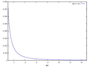
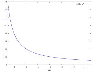
Figure 1: The deviation of $\rho$ parameter (left) and $\Delta g_{1}^{Z}=\Delta\kappa_{Z}$ (right) as a function of KK scale are plotted.

4 Summary

In this paper, we study the $\rho$ parameter and TGCs in the gauge-Higgs unification scenario. Although they are constants in the SM, these couplings or parameter in this model may become nonlinear functions of VEV $v$. It is due to the fact that the translational invariance along with the fifth dimension of this theory is broken down by the brane-localized mass term. In fact, we have derived the analytic expressions for the $\rho$ parameter and TGCs by use of the exact mode functions and its mass eigenvalues which are given by solving EOM of the neutral gauge bosons. It indicates that they are the function of the VEV $v$. We furthermore have verified that they reduce to the SM predictions in the limit where the nonlinearity of $v$ can be neglected. It is quite natural since the VEV $v$ in this scenario is embedded in the Wilson line phase and it becomes unit matrix in that limit.

These deviations are significant in the phenomenological point of view, because the $\rho$ parameter and TGCs are precisely measured by experiments. We have performed the numerical study and obtained the lower bound of the compactification scale $R^{-1}>3{\rm TeV}$. A severer constraint $R^{-1}>6.3{\rm TeV}$ is obtained by combining Higgs production data at LHC. We hope that this result will provide useful information for new physics search at LHC Run 2 or ILC in a future.

Appendix A Derivation of mode functions and its KK mass spectrum

In this appendix, we derive the KK mass spectrum of the neutral gauge boson. As pointed in the main text, there are two kinds of mixings which arise from the brane localized gauge boson mass term and the VEV of the higgs $A_{y}^{6}$. We completely solve these mixings by factoring out the VEV from mode equations. The mass spectrums are determined by the boundary conditions on the mode functions and its derivatives.

A.1 charged gauge boson

The charged gauge boson $W^{\pm}_{\mu}$ in our model corresponds to the $A^{1}_{\mu},A^{2}_{\mu},A^{4}_{\mu},A^{5}_{\mu}$ of the $SU(3)_{W}$. Their EOM are already derived as eq(A.1) and eq(A.2) in the main text.

$$-m^{2}A=(\partial_{y}+M_{W}M_{\rm C})(\partial_{y}+M_{W}M_{\rm C})A$$ (A.1)

where

$$M_{\rm C}=\begin{pmatrix}0&0&0&-1\\ 0&0&+1&0\\ 0&-1&0&0\\ +1&0&0&0\end{pmatrix}\,.$$ (A.2)

Note that we adopt the matrix form $A=(A^{1}_{\mu},A^{2}_{\mu},A^{4}_{\mu},A^{5}_{\mu})^{\rm T}$. Let us first eliminate the $M_{W}$ from the EOM (A.1) by defining $A={\rm e}^{-M_{W}M_{\rm C}y}{\tilde{A}}$, then the EOM becomes

$$-\partial_{y}^{2}\tilde{A}=m^{2}\tilde{A}$$ (A.3)

We require the $Z_{2}$ conditions at the origin and periodicity on the gauge bosons. The $Z_{2}$ BCs are the same for both $A$ and $\tilde{A}$ because of the phase matrix $\exp\left[-M_{W}M_{\rm C}y\right]$ becomes unit matrix at the origin, the $Z_{2}$ condition at the origin $\tilde{A}(x^{\mu},y)={\rm diag}(+,+,-,-)\tilde{A}(x^{\mu},-y)$. From the $Z_{2}$ condition, the eq (A.3) is solved as

$$\begin{cases}\displaystyle A^{1}_{\mu}(x^{\mu},y)=\sum_{n}\left[\cos M_{W}y\cos my\tilde{A}^{1(n)}_{\mu}(x^{\mu})+\sin M_{W}y\sin my\tilde{A}^{5(n)}_{\mu}(x^{\mu})\right]\\ \displaystyle A^{2}_{\mu}(x^{\mu},y)=\sum_{n}\left[\cos M_{W}y\cos my\tilde{A}^{2(n)}_{\mu}(x^{\mu})-\sin M_{W}y\sin my\tilde{A}^{4(n)}_{\mu}(x^{\mu})\right]\\ \displaystyle A^{4}_{\mu}(x^{\mu},y)=\sum_{n}\left[\cos M_{W}y\sin my\tilde{A}^{4(n)}_{\mu}(x^{\mu})+\sin M_{W}y\cos my\tilde{A}^{2(n)}_{\mu}(x^{\mu})\right]\\ \displaystyle A^{5}_{\mu}(x^{\mu},y)=\sum_{n}\left[\cos M_{W}y\sin my\tilde{A}^{5(n)}_{\mu}(x^{\mu})-\sin M_{W}y\cos my\tilde{A}^{1(n)}_{\mu}(x^{\mu})\right]\end{cases}$$ (A.4)

where ${\rm e}^{-M_{W}M_{\rm C}y}=\cos M_{W}y-M_{\rm C}\sin M_{W}y$ is used.

From the periodicity at $y=\pi R$, $A(x^{\mu},\pi R)=A(x^{\mu},-\pi R)$, we have

$$\begin{cases}\cos\hat{M}_{W}\sin\hat{m}\tilde{A}^{4(n)}+\sin\hat{M}_{W}\cos\hat{m}\tilde{A}^{2(n)}=0\\ \cos\hat{M}_{W}\sin\hat{m}\tilde{A}^{5(n)}-\sin\hat{M}_{W}\cos\hat{m}\tilde{A}^{1(n)}=0\end{cases}$$ (A.5)

where the $\hat{m}$ describes $\pi Rm$. To satisfy the EOM at $y=\pi R$, we impose a conditions

$$0=\lim_{\epsilon\to 0}\int_{\pi R-\epsilon}^{\pi R+\epsilon}{\rm d}y\left[m^{2}+(\partial_{y}+M_{W}M_{\rm C})(\partial_{y}+M_{W}M_{\rm C})\right]A\,.$$ (A.6)

Since the gauge boson fields $A$ is continuous at $y=\pi R$, the above condition becomes

$$0=\left[{\rm e}^{-M_{W}M_{\rm C}y}\partial_{y}\tilde{A}\right]^{\pi R}_{-\pi R}\,$$ (A.7)

in the matrix form, or

$$\begin{cases}0=-\cos\hat{M}_{W}\sin\hat{m}\tilde{A}^{1(n)}-\sin\hat{M}_{W}\cos\hat{m}\tilde{A}^{5(n)}\,,\\ 0=-\cos\hat{M}_{W}\sin\hat{m}\tilde{A}^{2(n)}+\sin\hat{M}_{W}\cos\hat{m}\tilde{A}^{4(n)}\,.\end{cases}$$ (A.8)

These conditions (A.5) and (A.8) determine the mass spectrum and its eigenstate. They are summarized in the following form.

$$0=\begin{bmatrix}-\tan\hat{m}&0&0&\tan\hat{M}_{W}\\ 0&\tan\hat{m}&\tan\hat{M}_{W}&0\\ -\tan\hat{M}_{W}&0&0&\tan\hat{m}\\ 0&\tan\hat{M}_{W}&\tan\hat{m}&0\end{bmatrix}\begin{pmatrix}\tilde{A}^{1(n)}\\ \tilde{A}^{2(n)}\\ \tilde{A}^{4(n)}\\ \tilde{A}^{5(n)}\end{pmatrix}\,.$$ (A.9)

The condition that determines the mass spectrum is equivalent to that the eq(A.9) has nontrivial solutions, namely, the determinant of the matrix in the eq(A.9) should be vanished. This gives two types of spectrum as

$$\tan\hat{m}=\pm\tan\hat{M}_{W}\,.$$ (A.10)

The charged gauge boson in the SM corresponds to the zero mode of KK modes, i.e. $m=\pm M_{W}$, the $A^{1}_{\mu}$ and $A^{2}_{\mu}$ is constant with respect to the fifth dimension. Thus we have

$$A^{1}_{\mu}(x^{\mu},y)\supset\frac{1}{\sqrt{2\pi R}}\frac{W^{+}_{\mu}(x^{\mu})+W^{-}_{\mu}(x^{\mu})}{\sqrt{2}},\displaystyle A^{2}_{\mu}(x^{\mu},y)\supset\frac{1}{\sqrt{2\pi R}}\frac{W^{-}_{\mu}(x^{\mu})-W^{+}_{\mu}(x^{\mu})}{\sqrt{2}i}.$$ (A.11)

Note that the factor $1/\sqrt{2\pi R}$ comes from the normalization.

A.2 neutral gauge boson

In this subsection, we focus on the neutral gauge boson. As we mentioned in the introduction, the $U(1)^{\prime}$ gauge boson and neutral sector in the $SU(3)_{W}$ are mixed by the boundary term. Similar to the main text, we treat the index of $U(1)^{\prime}$ gauge boson as $a=0$. Adopting the vector notation $A=(A^{0}_{\mu},A^{3}_{\mu},A^{7}_{\mu},A^{8}_{\mu})^{\rm T}$, the EOM for the neutral gauge boson are given by

$$-m^{2}A=(\partial_{y}+2M_{W}M_{\rm N})(\partial_{y}+2M_{W}M_{\rm N})A+\pi RM_{G}^{2}[\delta(y)+\delta(y-\pi R)]U^{\dagger}{\rm diag}(1,0,0,0)UA$$ (A.12)

where the $M_{G}$ stands for the brane-localized mass term for the anomalous gauge boson. The matrices $M_{\text{N}}$ and $U$ are defined by

$$M_{\rm N}=\begin{pmatrix}0&0&0&0\\ 0&0&\frac{1}{2}&0\\ 0&-\frac{1}{2}&0&\frac{\sqrt{3}}{2}\\ 0&0&-\frac{\sqrt{3}}{2}&0\end{pmatrix}\,,\,\,U=\begin{pmatrix}\cos\theta&0&0&-\sin\theta\\ 0&1&0&0\\ 0&0&1&0\\ \sin\theta&0&0&\cos\theta\end{pmatrix}\,.$$ (A.13)

Eliminating $M_{W}$ by using

$$A={\rm e}^{-2M_{W}M_{\rm N}y}U^{\dagger}\hat{A}$$ (A.14)

in a similar way of the analysis done for the charged gauge boson, the above EOM becomes

$$-m^{2}\hat{A}=\partial_{y}^{2}\hat{A}+\pi RM_{G}^{2}[\delta(y)+\delta(y-\pi R)]U{\rm e}^{2M_{W}M_{\rm N}y}U^{\dagger}{\rm diag}(1,0,0,0)U{\rm e}^{-2M_{W}M_{\rm N}y}U^{\dagger}\hat{A}\,.$$ (A.15)

It is useful to expand the phase matrix in the following form:

$${\rm e}^{-2M_{W}M_{\rm N}y}=\begin{pmatrix}1&0&0&0\\ 0&\frac{3}{4}+\frac{1}{4}\cos 2M_{W}y&-\frac{1}{2}\sin 2M_{W}y&\frac{\sqrt{3}}{4}(1-\cos 2M_{W}y)\\ 0&\frac{1}{2}\sin 2M_{W}y&\cos 2M_{W}y&-\frac{\sqrt{3}}{2}\sin 2M_{W}y\\ 0&\frac{\sqrt{3}}{4}(1-\cos 2M_{W}y)&\frac{\sqrt{3}}{2}\sin 2M_{W}y&\frac{1}{4}+\frac{3}{4}\cos 2M_{W}y\end{pmatrix}\,.$$

Next, we consider the boundary conditions (BCs) at $y=0$ and $\pi R$. We require the $Z_{2}$ condition at the origin and periodicity similar to those for the charged gauge boson. Since the $Z_{2}$ condition on the $\hat{A}$ are the same as those on the $A$, the mode functions $f^{b}(y)$ satisfy

$$f(y)={\rm diag}(+,+,-,+)f(-y)\,.$$ (A.16)

where $f(y)$ is defined through $\hat{A}^{b}_{\mu}(x^{\mu},y)=\hat{A}^{b}_{\mu}(x^{\mu})f^{b}(y)$. By taking into account the condition, the EOM (A.15) are immediately solved in the bulk as follows;

$$f^{b}(y)\propto\begin{cases}\cos(m|y|-\alpha_{b})&\text{for }b=0,3,8\\ \sin(my)&\text{for }b=7\end{cases}$$ (A.17)

where $\alpha_{b}$ stand for the phases.

Since the delta functions are present at $y=0$ and $\pi R$, the first derivative of the mode functions becomes discontinuous. The conditions for the discontinuity are derived by integrating out the EOM (A.15) around $y=0$ and $\pi R$. Taking into account the continuous condition at the origin $\lim_{\epsilon\to 0}\left[A(x,\epsilon)-A(x,-\epsilon)\right]=0$, we have

$$0=\lim_{\varepsilon\to 0}[\partial_{y}f^{a}(x,y)]_{-\varepsilon}^{\varepsilon}+\pi RM_{G}^{2}f^{a}\delta_{a0}\,.$$ (A.18)

Note that the index $a$ in the second term does not mean the summation. Summarizing the solutions, we find

$$\begin{cases}f^{0}\propto\cos(m|y|-\alpha)\\ f^{3}\propto\cos my\\ f^{7}\propto\sin my\\ f^{8}\propto\cos my\end{cases}\,,\,2\hat{m}\sin\alpha+\hat{M}_{G}^{2}\cos\alpha=0$$ (A.19)

where $\hat{m}=\pi Rm$ and $\hat{M}_{G}=\pi RM_{G}$ . Same procedure further applies to $y=\pi R$ case. We integrate out eq (A.15) around $\pi R-\varepsilon<y<\pi R+\varepsilon$, it becomes

$$0= \lim_{\epsilon\to 0}[\partial_{y}A]_{\pi R-\varepsilon}^{\pi R+\varepsilon}+\pi RM_{G}^{2}U^{\dagger}\text{diag}(1,0,0,0)UA(x,\pi R)$$

$$= -2{\rm e}^{-2M_{W}M_{\rm N}y}U^{\dagger}\partial_{y}\hat{A}(x,y)|_{y=\pi R}^{\text{odd}}+\pi RM_{G}^{2}U^{\dagger}\text{diag}(1,0,0,0)UA(x,y)|^{\text{even}}_{y=\pi R}\,.$$ (A.20)

The first (second) term stands for putting $y=\pi R$ after extracting the odd (even) function. Therefore we have following three relations.

$$0= \Big{[}-\cos\theta\hat{m}\sin(\hat{m}-\alpha)-\frac{1}{2}\hat{M}_{G}^{2}\cos\theta(1-\frac{3}{4}\sin^{2}\theta(1-\cos 2\hat{M}_{W}))\cos(\hat{m}-\alpha),$$

$$~{}\frac{\sqrt{3}}{8}\hat{M}_{G}^{2}\sin\theta\cos\theta(1-\cos 2\hat{M}_{W})\cos\hat{m},\frac{\sqrt{3}}{4}\hat{M}_{G}^{2}\sin\theta\cos\theta\sin 2\hat{M}_{W}\sin\hat{m},$$

$$~{}-\sin\theta\hat{m}\sin\hat{m}-\frac{3}{8}\hat{M}_{G}^{2}\sin\theta\cos^{2}\theta(1-\cos 2\hat{M}_{W})\cos\hat{m}\Big{]}\hat{A}(x)\,,$$ (A.21)

$$0= \Big{[}\frac{\sqrt{3}}{4}\sin\theta(1-\cos 2\hat{M}_{W})\sin(\hat{m}-\alpha),-(\frac{3}{4}+\frac{1}{4}\cos 2\hat{M}_{W})\sin\hat{m},$$

$$~{}-\frac{1}{2}\sin 2\hat{M}_{W}\cos\hat{m},-\frac{\sqrt{3}}{4}\cos\theta(1-\cos 2\hat{M}_{W})\sin\hat{m}\Big{]}\hat{A}(x)\,,$$ (A.22)

$$0= \Big{[}\sin\theta(\frac{1}{4}+\frac{3}{4}\cos 2\hat{M}_{W})\hat{m}\sin(\hat{m}-\alpha)+\frac{1}{2}\hat{M}_{G}^{2}\sin\theta(1-\frac{3}{4}\sin^{2}\theta(1-\cos 2\hat{M}_{W}))\cos(\hat{m}-\alpha),$$

$$~{}-\frac{\sqrt{3}}{4}(1-\cos 2\hat{M}_{W})\hat{m}\sin\hat{m}-\frac{\sqrt{3}}{8}\hat{M}_{G}^{2}\sin^{2}\theta(1-\cos 2\hat{M}_{W})\cos\hat{m},$$

$$~{}\frac{\sqrt{3}}{2}\sin 2\hat{M}_{W}\hat{m}\cos\hat{m}-\frac{\sqrt{3}}{4}\hat{M}_{G}^{2}\sin^{2}\theta\sin 2\hat{M}_{W}\sin\hat{m},$$

$$~{}-\cos\theta(\frac{1}{4}+\frac{3}{4}\cos 2\hat{M}_{W})\hat{m}\sin\hat{m}+\frac{3}{8}\hat{M}_{G}^{2}\sin^{2}\theta\cos\theta(1-\cos 2\hat{M}_{W})\cos\hat{m}\Big{]}\hat{A}(x)\,.$$ (A.23)

Next we consider the BCs at $y=\pi R$. The mode functions are continuous at $y=\pi R$ due to the fact that the theory is invariant under the translation along the extra dimension, namely,

$$0= \lim_{\epsilon\to 0}\left[A(x,\pi R+\epsilon)-A(x,\pi R-\epsilon)\right]=\lim_{\epsilon\to 0}\left[A(x,-\pi R+\epsilon)-A(x,\pi R-\epsilon)\right]$$ (A.24)

$$= -A(x,y)|^{\text{odd}}_{y=\pi R}$$ (A.25)

$$= \begin{pmatrix}0\\ 0\\ \frac{1}{2}\sin 2\hat{M}_{W}\cos\hat{m}\hat{A}^{3}+\cos 2\hat{M}_{W}\sin\hat{m}\hat{A}^{7}-\frac{\sqrt{3}}{2}\sin 2\hat{M}_{W}(\cos\theta\cos\hat{m}\hat{A}^{8}-\sin\theta\cos(\hat{m}-\alpha)\hat{A}^{0})\\ 0\end{pmatrix}.$$ (A.26)

In the first line, $\pi R+\epsilon$ is replaced with $-\pi R+\epsilon$ by respecting the translational invariance. Expressing by the matrix form, we have

$$0=[\frac{\sqrt{3}}{2}\sin 2\hat{M}_{W}\sin\theta\cos(\hat{m}-\alpha),\frac{1}{2}\sin 2\hat{M}_{W}\cos\hat{m},\cos 2\hat{M}_{W}\sin\hat{m},-\frac{\sqrt{3}}{2}\cos\theta\sin 2\hat{M}_{W}\cos\hat{m}]\hat{A}\,.$$ (A.27)

To summarize, the (A.2)-(A.2) and (A.27) give the mass eigenstate and its mass spectrum. We subtract them as $(\ref{masscondition4})+\tan(\theta)\times(\ref{masscondition2})+\sqrt{3}\times(\ref{masscondition3})$ for simplicity. Replacing $\hat{M}_{G}^{2}$ with $-2\hat{m}\tan\alpha$, we have

$$0=[0,-\sqrt{3}\sin\hat{m},0,-\frac{1}{\cos\theta}\sin\hat{m}]\hat{A}.$$ (A.28)

By multiplying $\cos\alpha$ by condition (A.2), we summarize the conditions (A.2)-(A.2) and (A.27) as

$$0= \Big{[}\frac{\sqrt{3}}{2}\sin 2\hat{M}_{W}\sin\theta\cos(\hat{m}-\alpha),\frac{1}{2}\sin 2\hat{M}_{W}\cos\hat{m},\cos 2\hat{M}_{W}\sin\hat{m},-\frac{\sqrt{3}}{2}\cos\theta\sin 2\hat{M}_{W}\cos\hat{m}\Big{]}\hat{A}\,,$$ (A.29)

$$0= \Big{[}-\cos\theta\sin(\hat{m}-2\alpha)-\frac{3}{4}\cos\theta\sin^{2}\theta\sin\alpha(1-\cos 2\hat{M}_{W})\cos(\hat{m}-\alpha),$$

$$~{}-\frac{\sqrt{3}}{4}\sin\alpha\sin\theta\cos\theta(1-\cos 2\hat{M}_{W})\cos\hat{m},-\frac{\sqrt{3}}{2}\sin\alpha\sin\theta\cos\theta\sin 2\hat{M}_{W}\sin\hat{m},$$

$$~{}-\sin\theta\cos\alpha\sin\hat{m}+\frac{3}{4}\sin\alpha\sin\theta\cos^{2}\theta(1-\cos 2\hat{M}_{W})\cos\hat{m}\Big{]}\hat{A}\,,$$ (A.30)

$$0= \Big{[}\frac{\sqrt{3}}{4}\sin\theta(1-\cos 2\hat{M}_{W})\sin(\hat{m}-\alpha),$$

$$~{}-(\frac{3}{4}+\frac{1}{4}\cos 2\hat{M}_{W})\sin\hat{m},-\frac{1}{2}\sin 2\hat{M}_{W}\cos\hat{m},-\frac{\sqrt{3}}{4}\cos\theta(1-\cos 2\hat{M}_{W})\sin\hat{m}\Big{]}\hat{A}\,,$$ (A.31)

$$0= \Big{[}0,-\sqrt{3}\sin\hat{m},0,-\frac{1}{\cos\theta}\sin\hat{m}\Big{]}\hat{A}$$ (A.32)

where $\tan\alpha=-\frac{\hat{M}_{G}^{2}}{2\hat{m}}$. Since the brane mass term for the gauge boson $\hat{M}_{G}$ is taken to be infinity($\alpha\to-\pi/2$), the above conditions become

$$0= \Big{[}-\frac{\sqrt{3}}{2}\sin 2\hat{M}_{W}\sin\theta\sin\hat{m},\frac{1}{2}\sin 2\hat{M}_{W}\cos\hat{m},\cos 2\hat{M}_{W}\sin\hat{m},-\frac{\sqrt{3}}{2}\cos\theta\sin 2\hat{M}_{W}\cos\hat{m}\Big{]}\hat{A}\,,$$ (A.33)

$$0= \Big{[}\sin\hat{m}-\frac{3}{4}\sin^{2}\theta(1-\cos 2\hat{M}_{W})\sin\hat{m},\frac{\sqrt{3}}{4}\sin\theta(1-\cos 2\hat{M}_{W})\cos\hat{m},$$

$$~{}\frac{\sqrt{3}}{2}\sin\theta\sin 2\hat{M}_{W}\sin\hat{m},-\frac{3}{4}\sin\theta\cos\theta(1-\cos 2\hat{M}_{W})\cos\hat{m}\Big{]}\hat{A}\,,$$ (A.34)

$$0= \Big{[}\frac{\sqrt{3}}{4}\sin\theta(1-\cos 2\hat{M}_{W})\cos\hat{m},-(\frac{3}{4}+\frac{1}{4}\cos 2\hat{M}_{W})\sin\hat{m},$$

$$~{}-\frac{1}{2}\sin 2\hat{M}_{W}\cos\hat{m},-\frac{\sqrt{3}}{4}\cos\theta(1-\cos 2\hat{M}_{W})\sin\hat{m}\Big{]}\hat{A}\,,$$ (A.35)

$$0= \Big{[}0,-\sqrt{3}\sin\hat{m},0,-\frac{1}{\cos\theta}\sin\hat{m}\Big{]}\hat{A}\,.$$ (A.36)

By adopting matrix notation, they become

$$N\hat{A}=0$$ (A.37)

where the matrix $N$ is defined by

$$N= \left[\begin{matrix}-\frac{\sqrt{3}}{2}\sin 2\hat{M}_{W}\sin\theta\sin\hat{m}&\frac{1}{2}\sin 2\hat{M}_{W}\cos\hat{m}\\ \sin\hat{m}-\frac{3}{4}\sin^{2}\theta(1-\cos 2\hat{M}_{W})\sin\hat{m}&\frac{\sqrt{3}}{4}\sin\theta(1-\cos 2\hat{M}_{W})\cos\hat{m}\\ \frac{\sqrt{3}}{4}\sin\theta(1-\cos 2\hat{M}_{W})\cos\hat{m}&-(\frac{3}{4}+\frac{1}{4}\cos 2\hat{M}_{W})\sin\hat{m}\\ 0&-\sqrt{3}\sin\hat{m}\end{matrix}\right.$$

$$~{}~{}~{}~{}~{}~{}~{}~{}~{}~{}~{}~{}~{}~{}~{}~{}~{}~{}~{}~{}~{}\left.\begin{matrix}\cos 2\hat{M}_{W}\sin\hat{m}&-\frac{\sqrt{3}}{2}\cos\theta\sin 2\hat{M}_{W}\cos\hat{m}\\ \frac{\sqrt{3}}{2}\sin\theta\sin 2\hat{M}_{W}\sin\hat{m}&-\frac{3}{4}\sin\theta\cos\theta(1-\cos 2\hat{M}_{W})\cos\hat{m}\\ -\frac{1}{2}\sin 2\hat{M}_{W}\cos\hat{m}&-\frac{\sqrt{3}}{4}\cos\theta(1-\cos 2\hat{M}_{W})\sin\hat{m}\\ 0&-\frac{1}{\cos\theta}\sin\hat{m}\end{matrix}\right]\,.$$ (A.38)

A.2.1 mass spectrum

To have the non-trivial solutions of eq(A.37), the mass eigenvalues are obtained from solving

$$\det N=0.$$ (A.39)

Then, we find solutions

$$\sin^{2}\hat{m}= 0\,,\,\tan\hat{m}=\pm\frac{\sqrt{4\cos^{2}\theta_{W}-\sin^{2}\hat{M}_{W}}}{2\cos^{2}\theta_{W}-\sin^{2}\hat{M}_{W}}\sin\hat{M}_{W}\,.$$ (A.40)

We note that the $\theta$ is replaced with $\theta_{W}$. The above result tells us that the neutral gauge bosons split to $\gamma,Z^{\prime}$ (first relation) and $Z$ boson (second relation) since the right hand side of the second relation reduce to $\frac{\hat{M}_{W}}{\cos\theta_{W}}$ in the limit where the nonlinearity of $v$ can be neglected.

A.2.2 mass eigenstate

To find out the mass eigenstate, we substitute the corresponding mass eigenvalue (A.40) for the conditions (A.37).

For the photon $\gamma$ and anomalous gauge boson $Z^{\prime}$, substituting $\sin\hat{m}=0$ with matrix $N$ leads to

$$\begin{pmatrix}0&\frac{1}{2}&0&-\frac{\sqrt{3}}{2}\cos\theta\\ 0&\frac{1}{2}&0&-\frac{\sqrt{3}}{2}\cos\theta\\ \frac{\sqrt{3}}{4}\sin\theta(1-\cos 2\hat{M}_{W})&0&-\frac{1}{2}\sin 2\hat{M}_{W}&0\end{pmatrix}\hat{A}=0$$ (A.41)

It gives two different eigenstates. They are included as

$$\begin{cases}\hat{A}^{3}_{\mu}\supset\sin\theta_{W}\gamma_{\mu}\,,\hat{A}^{8}_{\mu}\supset\cos\theta_{W}\gamma_{\mu}\\ \hat{A}^{0}_{\mu}\supset\frac{2\cos\theta_{W}\cos\hat{M}_{W}}{\sqrt{4\cos^{2}\theta_{W}-\sin^{2}\hat{M}_{W}}}Z^{\prime}_{\mu}\,,\hat{A}^{7}_{\mu}\supset\frac{\sqrt{4\cos^{2}\theta_{W}-1}}{\sqrt{4\cos^{2}\theta_{W}-\sin^{2}\hat{M}_{W}}}\sin\hat{M}_{W}Z^{\prime}_{\mu}\end{cases}$$ (A.42)

where $\theta$ is replaced with $\theta_{W}$. They are distinguished by taking the limit $\hat{M}_{W}\to 0$, namely, the anomalous gauge boson $Z^{\prime}_{\mu}$ is exactly the same as $\hat{A}^{0}_{\mu}$ in the limit due to the absence of the mixings by the VEV $v$. They are also identified by taking the limit $\cos\theta_{W}\to 1/2\,(\theta\to 0)$ since the brane-localized gauge boson mass term $M_{G}$ merely couples to $A^{0}_{\mu}$.

For the $Z$ boson, substituting the second relation in the eq(A.40) with (A.37) leads to

$$\begin{cases}\hat{A}^{0}_{\mu}\supset\pm\sqrt{\frac{4\cos^{2}\theta_{W}-1}{2(4\cos^{2}\theta_{W}-\sin^{2}\hat{M}_{W})}}\sin\hat{M}_{W}Z_{\mu}\,,\\ \hat{A}^{3}_{\mu}\supset\frac{1}{\sqrt{2}}\cos\theta_{W}Z_{\mu}\,,\\ \hat{A}^{7}_{\mu}\supset\mp\frac{\sqrt{2}\cos\theta_{W}\cos\hat{M}_{W}}{\sqrt{4\cos^{2}\theta_{W}-\sin^{2}\hat{M}_{W}}}Z_{\mu}\,,\\ \hat{A}^{8}_{\mu}\supset-\frac{1}{\sqrt{2}}\sin\theta_{W}Z_{\mu}\,.\end{cases}$$ (A.43)

The normalized mode functions are

$$\begin{cases}f^{0}=-\frac{1}{\sqrt{\pi R-\frac{1}{2m}\sin 2\pi Rm}}\sin m|y|\,,\\ f^{3}=\frac{1}{\sqrt{\pi R+\frac{1}{2m}\sin 2\pi Rm}}\cos my\,,\\ f^{7}=\frac{1}{\sqrt{\pi R-\frac{1}{2m}\sin 2\pi Rm}}\sin my\,,\\ f^{8}=\frac{1}{\sqrt{\pi R+\frac{1}{2m}\sin 2\pi Rm}}\cos my\,.\end{cases}$$ (A.44)

The mass eigenvalues $m$ are understood to be substituted by the corresponding ones. We then finally solve the mixings as follows.

$$\begin{pmatrix}A^{0}\\ A^{3}\\ A^{7}\\ A^{8}\end{pmatrix}= \begin{pmatrix}\cos\theta\hat{A}^{0}+\sin\theta\hat{A}^{8}\\ (\frac{3}{4}+\frac{1}{4}\cos 2M_{W}y)\hat{A}^{3}-\frac{1}{2}\sin 2M_{W}y\hat{A}^{7}+\frac{\sqrt{3}}{4}(1-\cos 2M_{W}y)(\cos\theta\hat{A}^{8}-\sin\theta\hat{A}^{0})\\ \frac{1}{2}\sin 2M_{W}y\hat{A}^{3}+\cos 2M_{W}y\hat{A}^{7}-\frac{\sqrt{3}}{2}\sin 2M_{W}y(\cos\theta\hat{A}^{8}-\sin\theta\hat{A}^{0})\\ \frac{\sqrt{3}}{4}(1-\cos 2M_{W}y)\hat{A}^{3}+\frac{\sqrt{3}}{2}\sin 2M_{W}y\hat{A}^{7}+(\frac{1}{4}+\frac{3}{4}\cos 2M_{W}y)(\cos\theta\hat{A}^{8}-\sin\theta\hat{A}^{0})\end{pmatrix}\,,$$ (A.45)

where $\cos\theta=\frac{\sin\theta_{W}}{\sqrt{3}\cos\theta_{W}},\sin\theta=\frac{\sqrt{4\cos^{2}\theta_{W}-1}}{\sqrt{3}\cos\theta_{W}}$.

Finally, we comment on the zero mode $Z$ boson. The mass spectrum of the KK mode $Z$ boson are split to $m_{Z}=\pm M_{Z}+\frac{n}{R}$ according to the condition shown in the eq(A.40). The $M_{Z}$ is a minimum value of $m_{z}$ which satisfy the above condition. So we distinguish them by noting $Z^{(n\pm)}$ but the zero mode $Z^{(0\pm)}$ is degenerate since its mass are $\pm M_{Z}$, respectively. We therefore regard the $Z^{(0+)}$ and $Z^{(0-)}$ as the SM $Z$ boson. Then, zero mode $Z$ boson can be read off as $Z^{(0\pm)}=\frac{1}{\sqrt{2}}Z$ to avoid the double counting.

In fact, the $Z^{(0\pm)}$ boson are included as

$$\begin{cases}\hat{A}^{0}\supset\pm\sqrt{\frac{4\cos^{2}\theta_{W}-1}{2(4\cos^{2}\theta_{W}-\sin^{2}\hat{M}_{W})}}\sin\hat{M}_{W}f^{0}_{\pm M_{Z}}Z^{(0\pm)}=\sqrt{\frac{4\cos^{2}\theta_{W}-1}{2(4\cos^{2}\theta_{W}-\sin^{2}\hat{M}_{W})}}\sin\hat{M}_{W}f^{0}_{M_{Z}}Z^{(0\pm)}\\ \hat{A}^{3}\supset\frac{1}{\sqrt{2}}\cos\theta_{W}f^{3}_{\pm M_{Z}}Z^{(0\pm)}=\frac{1}{\sqrt{2}}\cos\theta_{W}f^{3}_{M_{Z}}Z^{(0\pm)}\\ \hat{A}^{7}\supset\mp\frac{\sqrt{2}\cos\theta_{W}\cos\hat{M}_{W}}{\sqrt{4\cos^{2}\theta_{W}-\sin^{2}\hat{M}_{W}}}f^{7}_{\pm M_{Z}}Z^{(0\pm)}=-\frac{\sqrt{2}\cos\theta_{W}\cos\hat{M}_{W}}{\sqrt{4\cos^{2}\theta_{W}-\sin^{2}\hat{M}_{W}}}f^{7}_{M_{Z}}Z^{(0\pm)}\\ \hat{A}^{8}\supset-\frac{1}{\sqrt{2}}\sin\theta_{W}f^{8}_{\pm M_{Z}}Z^{(0\pm)}=-\frac{1}{\sqrt{2}}\sin\theta_{W}f^{8}_{M_{Z}}Z^{(0\pm)}\\ \end{cases}$$ (A.46)

where $f^{i}_{\pm M_{Z}}=f^{i}|_{m=\pm M_{Z}}$. Then, the quadratic form becomes $(\hat{A}^{0})^{2}+(\hat{A}^{3})^{2}+(\hat{A}^{7})^{2}+(\hat{A}^{8})^{2}=(Z^{(0+)})^{2}+(Z^{(0-)})^{2}=Z^{2}$ and thus we have $Z^{(0\pm)}=\frac{1}{\sqrt{2}}Z$.

References

- [1] N. S. Manton, Nucl. Phys. B 158, 141 (1979); D. B. Fairlie, Phys. Lett. B 82, 97 (1979), J. Phys. G 5, L55 (1979); Y. Hosotani, Phys. Lett. B 126, 309 (1983), Phys. Lett. B 129, 193 (1983), Annals Phys. 190, 233 (1989).
- [2] H. Hatanaka, T. Inami and C. S. Lim, Mod. Phys. Lett. A 13, 2601 (1998).
- [3] I. Antoniadis, K. Benakli and M. Quiros, New J. Phys. 3, 20 (2001); G. von Gersdorff, N. Irges and M. Quiros, Nucl. Phys. B 635, 127 (2002); R. Contino, Y. Nomura and A. Pomarol, Nucl. Phys. B 671, 148 (2003); C. S. Lim, N. Maru and K. Hasegawa, J. Phys. Soc. Jap. 77, 074101 (2008); C. S. Lim, N. Maru and T. Miura, arXiv:1402.6761 [hep-ph]; K. Hasegawa, C. S. Lim and N. Maru, Phys. Lett. B 604, 133 (2004).
- [4] N. Maru and T. Yamashita, Nucl. Phys. B 754, 127 (2006); Y. Hosotani, N. Maru, K. Takenaga and T. Yamashita, Prog. Theor. Phys. 118, 1053 (2007).
- [5] C. S. Lim and N. Maru, Phys. Rev. D 75, 115011 (2007).
- [6] N. Maru, Mod. Phys. Lett. A 23, 2737 (2008); N. Maru and N. Okada, Phys. Rev. D 77, 055010 (2008); Phys. Rev. D 87, no. 9, 095019 (2013); Phys. Rev. D 88, no. 3, 037701 (2013); arXiv:1310.3348 [hep-ph].
- [7] Y. Adachi, C. S. Lim and N. Maru, Phys. Rev. D 76, 075009 (2007); Phys. Rev. D 79, 075018 (2009); Phys. Rev. D 80, 055025 (2009).
- [8] Y. Adachi, N. Kurahashi, C. S. Lim and N. Maru, JHEP 1011, 150 (2010); JHEP 1201, 047 (2012); Y. Adachi, N. Kurahashi, N. Maru and K. Tanabe, Phys. Rev. D 85, 096001 (2012); Y. Adachi, N. Kurahashi and N. Maru, arXiv:1404.4281 [hep-ph].
- [9] K. Hasegawa, N. Kurahashi, C. S. Lim and K. Tanabe, Phys. Rev. D 87, 016011 (2013).
- [10] Y. Hosotani and Y. Kobayashi, Phys. Lett. B 674, 192 (2009); Y. Hosotani, P. Ko and M. Tanaka, Phys. Lett. B 680, 179 (2009) , Y. Hosotani and Y. Sakamura, Prog. Theor. Phys. 118, 935 (2007).
- [11] Y. Adachi and N. Maru, Eur. Phys. J. Plus 130, no. 8, 168 (2015).
- [12] C. A. Scrucca, M. Serone and L. Silvestrini, Nucl. Phys. B 669, 128 (2003).
- [13] G. Cacciapaglia, C. Csaki and S. C. Park, JHEP 0603 (2006) 099.
- [14] M. López-Osorio, E. Martínez-Pascual, J. Montaño, H. Novales-Sánchez, J. J. Toscano and E. S. Tututi, Phys. Rev. D 88, no. 1, 016010 (2013).
- [15] V. M. Abazov et al. [D0 Collaboration], Phys. Lett. B 718, 451 (2012).
- [16] T. Corbett, O. J. P. Éboli, J. Gonzalez-Fraile and M. C. Gonzalez-Garcia, Phys. Rev. Lett. 111, 011801 (2013) .