Comments on: “A Random Forest Guided Tour” by G. Biau and E. Scornet

Abstract

This paper is a comment on the survey paper by Biau and Scornet (2016) about random forests. We focus on the problem of quantifying the impact of each ingredient of random forests on their performance. We show that such a quantification is possible for a simple pure forest, leading to conclusions that could apply more generally. Then, we consider “hold-out” random forests, which are a good middle point between “toy” pure forests and Breiman’s original random forests.

We would like to thank G. Biau and E. Scornet for their clear and thought-provoking survey (Biau and Scornet, 2016). It shows that for understanding better random forests mechanisms, we must go beyond consistency results and quantify the impact of each ingredient of random forests on their performance.

In this comment, we prove that such a quantification is possible for a simple pure forest, leading to conclusions that could apply more generally (Section 1). Then, we consider in Section 2 “hold-out” random forests, which are a good middle point between “toy” pure forests and Breiman’s original random forests.

1 Aggregation, two kinds of randomization and resampling

As clearly shown by Biau and Scornet (2016), two key ingredients of random forests are the aggregation process (several trees are combined to get the final estimator) and the diversity of the trees that are aggregated. We can distinguish two sources of diversity:

• randomization of the partition $\mathcal{P}_{\mathrm{final}}$,

• randomization of the labels, that is, of the predicted value in each cell of $\mathcal{P}_{\mathrm{final}}$, given $\mathcal{P}_{\mathrm{final}}$.

In Breiman’s random forests, resampling acts on the two kinds of randomization, while the choice of $\mathcal{M}_{\mathrm{try}}$ at each node of each tree acts on the randomization of the partitions only. In purely random forests, partitions are built independently from the data, so resampling (if any) only acts on the randomization of the labels. Therefore, the role of each kind of randomization is easier to understand, and to quantify separately, for purely random forests. In this section, we propose to do so for the one-dimensional toy forest introduced by Arlot and Genuer (2014, Section 4).

1.1 Toy forest

We first define the toy forest model, assuming that $\mathcal{X}=[0,1]$. Let $2\leq k\leq a\leq n$ be some integers. The partition associated to each tree is given by

$$\left[0,\frac{1-T}{k}\right),\,\left[\frac{1-T}{k},\frac{2-T}{k}\right),\,\ldots,\left[\frac{k-1-T}{k},\frac{k-T}{k}\right),\,\left[\frac{k-T}{k},1\right)$$

with $T\sim\mathcal{U}([0,1])$. Then, for each tree, a subsample $(X_{i},Y_{i})_{i\in I}$ of size $a$ is chosen (uniformly over the subsamples of size $a$), independently from $T$. The tree estimator is defined as usual: the predicted value at $\mathbf{x}$ is the average of the $Y_{i}$ such that $X_{i}$ belongs to $A_{n}(x;T)$, the cell of the partition that contains $\mathbf{x}$. Finally, the forest estimator is obtained by averaging $M\geq 1$ trees, where the trees are independent conditionally to $\mathcal{D}_{n}$.

Assume that $X_{i}\sim\mathcal{U}([0,1])$, the $(X_{i},Y_{i})$ are independent with the same distribution, the noise-level $\mathbb{E}[(Y-m(X))^{2}\,|\,X]=\sigma^{2}$ is constant, $m$ is of class $\mathcal{C}^{3}$, $n\gg 1$ and $a\gg k\log(n)$. Let $\mathbf{x}\in[k^{-1},1-k^{-1}]$ (to avoid border effects, see Arlot and Genuer (2014) for details) be fixed. Then, Table 1 provides the order of magnitude of

$$\mathbb{E}\Bigl{[}\bigl{(}m_{M,n}^{\mathrm{toy}}(\mathbf{x})-m(\mathbf{x})\bigr{)}^{2}\Bigr{]}\enspace,$$

the quadratic risk at $\mathbf{x}$ of a toy forest $m_{M,n}^{\mathrm{toy}}$ with $M$ trees, in various situations: with or without aggregation ($M=+\infty$ or $M=1$), with or without randomization of the partitions (we remove randomization of partitions by putting $T=0$ for all trees). Subsampling can also be removed by taking $a=n$ in all formulas. Note that in Table 1, the risk is written as the sum of an approximation error and an estimation error, see Appendix A. The main lines of the proof are given in Appendix B.

Table 1: Order of magnitude of the quadratic risk at $\mathbf{x}$ (approximation error + estimation error) for the one-dimensional toy random forest combined with subsampling without replacement; $a$ denotes the subsample size, $1/k$ is the size of each cell in a partition, see Appendix B for precise assumptions and approximations. The impact of subsampling can be quantified by comparing $a=n$ with $a<n$ in each formula.

	Single tree	Infinite forest
No randomization of partitions	$\displaystyle\frac{c_{1}(m,\mathbf{x})}{k^{2}}+\frac{\sigma^{2\vphantom{{}^{2}}}k}{a}$	$\displaystyle\frac{c_{1}(m,\mathbf{x})}{k^{2}\vphantom{{}_{3}}}+\frac{\sigma^{2}k}{n}$
Randomization of partitions	$\displaystyle\frac{c_{1}(m,\mathbf{x})}{k^{2}}+\frac{\sigma^{2\vphantom{{}^{2}}}k}{a}$	$\displaystyle\frac{c_{2}(m,\mathbf{x})}{k^{4}\vphantom{{}_{3}}}+\frac{2\sigma^{2}k}{3n}$

$$\text{where}\qquad c_{1}(m,\mathbf{\mathbf{x}})=\frac{m^{\prime}(\mathbf{x})^{2}}{12}\qquad\text{and}\qquad c_{2}(m,\mathbf{\mathbf{x}})=\frac{m^{\prime\prime}(\mathbf{x})^{2}}{144}\enspace.$$

Table 1 allows to quantify the impact of aggregation, randomization of the partitions, randomization of the labels—and their combinations—on the performance of toy forests:

• aggregation: comparing the two columns of Table 1 shows that aggregation always improve the performance (which is true for any forest model, by Jensen’s inequality). The improvement can be huge: when partitions and labels are randomized, $a\ll n$ and $k\gg 1$, both approximation and estimation errors decrease by an order of magnitude.

• randomization of the partitions: comparing the two lines of Table 1 shows that randomizing the partitions strongly improves the performance of the infinite forest (there is no change for a single tree, of course). The approximation error decreases by an order of magnitude, as previously showed by Arlot and Genuer (2014). The estimation error also decreases—as showed by Genuer (2012) for another pure forest—, but by a factor $3/2$ only.

• randomization of the labels: comparing $a=n$ with $a\ll n$ in the formulas of Table 1 shows the influence of subsampling, which is the only randomization mechanism for the labels. Single trees perform worse when $a<n$ (as expected since the sample size is lowered). The performance of infinite forests does not change with subsampling, which might seem a bit surprising given several results mentioned by Biau and Scornet (2016). This phenomenon corresponds to the fact that subagging does not improve a stable estimator (Bühlmann and Yu, 2002), and that a regular histogram is stable. Section 1.2 below explains why there is no contradiction with the random forests literature.

1.2 Discussion

Section 1.1 sheds some light on previous theoretical results on random forests, and suggests a few conjectures which deserve to be investigated.

Parametrization of the trees.

The end of Section 3.1 of Biau and Scornet’s survey might seem contradictory with the above results for the toy forest. According to most papers in the literature, “random forests reduce the estimation error of a single tree, while maintaining the same approximation error”. Moreover, an infinite forest can be consistent even when a single tree (grown with a sample of size $n$) is not. Table 1 precisely shows the opposite situation: the estimation error is almost the same for a single tree and for an infinite forest, while the approximation error is dramatically smaller for an infinite forest. In addition, when an infinite forest is consistent, $1\ll k\ll n$ hence a single tree trained with $a=n$ points is also consistent.

The point is that these results and ours consider different parametrizations of the trees. In Section 1.1, trees are parametrized by the number of leaves $k+1$; so, when comparing a tree with a forest, we think fair to compare (i) a tree of $k+1$ leaves trained with $n$ data points, with (ii) a forest where each tree has $k+1$ leaves and is trained with $a$ data points. In the literature, trees are often parametrized by the number $\mathtt{nodesize}$ of data points per cell. Then, comparisons are done between (i) a tree of $\approx n/\mathtt{nodesize}$ leaves trained with $n$ data points, and (ii) a forest where each tree has $\approx a/\mathtt{nodesize}$ leaves and is trained with $a$ data points. So, if we take $k\approx a/\mathtt{nodesize}$, the two approaches consider (approximately) the same forest (ii), but the reference trees (i) are quite different.

We do not mean that one of these two parametrizations is definitely better than the other: $\mathtt{nodesize}$ is a natural parameter for Breiman’s random forests, while toy forests are naturally parametrized by their number of leaves. Nevertheless, one must keep in mind that any comparison between a forest and a single tree trained with the full sample does depend on the parametrization.

The parametrization by $\mathtt{nodesize}$ can also hide some difficulties. For the toy forest model, $k$ has to be chosen, and this is not an easy task. One could think that this problem is solved by taking the $\mathtt{nodesize}$ parametrization with, say, $\mathtt{nodesize}=1$. This is wrong because we then have to choose the subsample size $a$, which is equivalent to the original problem since $k\approx a/\mathtt{nodesize}$.

What about Breiman’s forests?

Section 1.1 suggests that for the toy forest, the most important ingredient in the tree diversity is the randomization of the partitions. We conjecture that this holds true for general random forests.

Nevertheless, we do not mean that the resampling step should always be discarded, since for Breiman’s random forests (for instance), resampling also acts on the randomization of the partitions. A key open problem is to quantify the relative roles of resampling and of the choice of $\mathcal{M}_{\mathrm{try}}$ on the randomization of the partitions. Section 2 below shows that “hold-out random forests” can be a good playground for such investigations.

Bootstrap or subsampling?

Another important question is the choice between the bootstrap and subsampling, which remains an open problem according to Biau and Scornet (2016).

We conjecture that Table 1 is also valid for the $a$ out of $n$ bootstrap, which would mean that bootstrap and subsampling are fully equivalent with respect to the randomization of the labels, with no impact on the performance of pure forests. Assuming this holds true, subsampling (with or without replacement) with $a\ll n$ remains interesting for reducing the computational cost—Table 1 only requires that $a\gg k\log(n)$.

A key open problem remains: compare bootstrap and subsampling with respect to the randomization of the partitions for Breiman’s random forests. Again, “hold-out random forests” described in Section 2 should be a good starting point for such a comparison.

2 Hold-out random forests

We now consider a more complex forest model, called hold-out random forests, which is close to Breiman’s random forests while being simpler to analyze. Hold-out random forests have been proposed by Biau (2012, Section 3) and appear in the experiments of Arlot and Genuer (2014, Section 7).

2.1 Definition

Hold-out random forests can be defined as follows. First, the data set $\mathcal{D}_{n}$ is split, once and for all, into two subsamples $\mathcal{D}_{n_{1}}^{1}$ and $\mathcal{D}_{n_{2}}^{2}$, of respective sizes $n_{1}$ and $n_{2}$, satisfying $n=n_{1}+n_{2}$. This split is done independently from $\mathcal{D}_{n}$. Then, conditionally to $(\mathcal{D}_{n_{1}}^{1},\mathcal{D}_{n_{2}}^{2})$, the $M$ trees are built independently as follows. The partition associated with the $j$-th tree is built as for Breiman’s random forests with $\mathcal{D}_{n_{1}}^{1}$ as data set. In other words, it is the partition $\mathcal{P}_{\mathrm{final}}$ defined by Biau and Scornet (2016, Algorithm 1) with training set $\mathcal{D}_{n_{1}}^{1}$ as an input. The $j$-th tree estimate at $\mathbf{x}$ is defined by

$$m^{\mathrm{hoRF}}_{n}\bigl{(}\mathbf{x};\Theta_{j},\mathcal{D}_{n_{1}}^{1},\mathcal{D}_{n_{2}}^{2}\bigr{)}:=\sum_{(X_{i},Y_{i})\in\mathcal{D}_{n_{2}}^{2}}\frac{\mathbf{1}_{X_{i}\in A_{n_{1}}(\mathbf{x};\Theta_{j},\mathcal{D}_{n_{1}}^{1})}Y_{i}}{N_{n_{2}}(\mathbf{x};\Theta_{j},\mathcal{D}_{n_{1}}^{1},\mathcal{D}_{n_{2}}^{2})}$$

where $A_{n_{1}}(\mathbf{x};\Theta_{j},\mathcal{D}_{n_{1}}^{1})$ is the cell of this partition that contains $\mathbf{x}$ and $N_{n_{2}}(\mathbf{x};\Theta_{j},\mathcal{D}_{n_{1}}^{1},\mathcal{D}_{n_{2}}^{2})$ is the number of points $(X_{i},Y_{i})\in\mathcal{D}_{n_{2}}^{2}$ such that $X_{i}\in A_{n_{1}}(\mathbf{x};\Theta_{j},\mathcal{D}_{n_{1}}^{1})$. Finally, the hold-out forest estimate is defined by

$$m^{\mathrm{hoRF}}_{M,n}\bigl{(}\mathbf{x};\Theta_{1\ldots M},\mathcal{D}_{n_{1}}^{1},\mathcal{D}_{n_{2}}^{2}\bigr{)}=\frac{1}{M}\sum_{j=1}^{M}m^{\mathrm{hoRF}}_{n}\bigl{(}\mathbf{x};\Theta_{j},\mathcal{D}_{n_{1}}^{1},\mathcal{D}_{n_{2}}^{2}\bigr{)}\,.$$

In the definition of $m^{\mathrm{hoRF}}_{M,n}$, the building of the partitions depends on the same parameters as Breiman’s random forests: $\mathtt{mtry}$, $\mathtt{nodesize}$, the fact that resampling can be done with or without replacement, and the resample size $a_{n_{1}}$. It is also possible to add another resampling step when assigning labels to the leaves of each tree with $\mathcal{D}_{n_{2}}^{2}$; we do not consider it here since Section 1 suggests that this would not change much the performance (at least for forests).

A key property of hold-out random forests is that they are purely random: the subsamples $\mathcal{D}_{n_{1}}^{1}$ and $\mathcal{D}_{n_{2}}^{2}$ are independent, hence the partition associated with the trees are independent from $\mathcal{D}_{n_{2}}^{2}$. Note however that each partition still depends on some data (through $\mathcal{D}_{n_{1}}^{1}$), hence it could adapt to some features of the data, such as the “sparsity” of the regression function, the non-uniformity over $\mathcal{X}$ of the smoothness of $m$, or the non-uniformity of the distribution of $X$. Therefore, hold-out random forests can capture much of the complexity of Breiman’s random forests, while being easier to analyze since they are purely random. In particular, we can apply the results proved in Appendix A (where our $\mathcal{D}_{n_{2}}^{2}$ is written $\mathcal{D}_{n}$, and our $\mathcal{D}_{n_{1}}^{1}$ is hidden in the relationship between $\Theta_{j}$ and the partition of the $j$-th tree). Then, the quadratic risk of $m^{\mathrm{hoRF}}_{M,n}$ can be (approximately) decomposed into the sum of an approximation error and an estimation error, and these two terms can be studied separately. For instance, the results of Arlot and Genuer (2014) can be applied in order to analyze the approximation error.

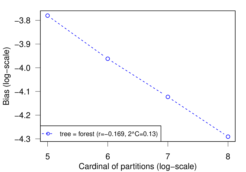
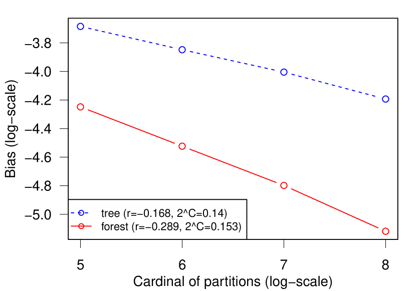
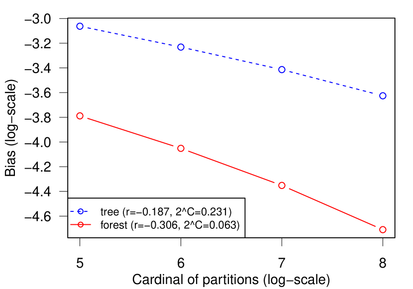
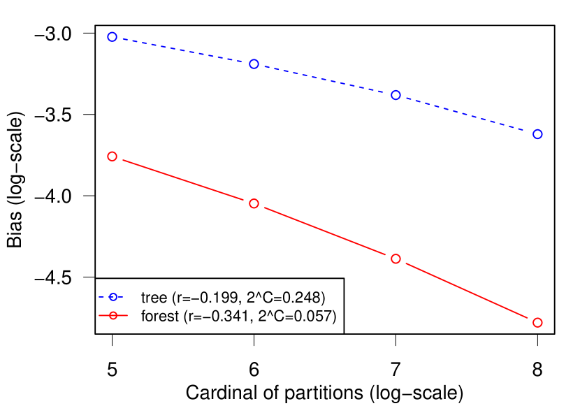
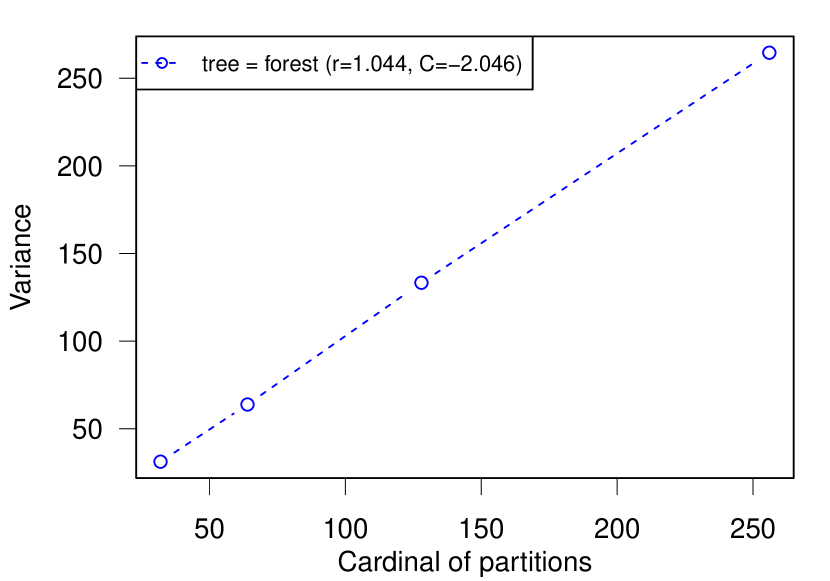
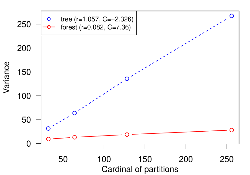
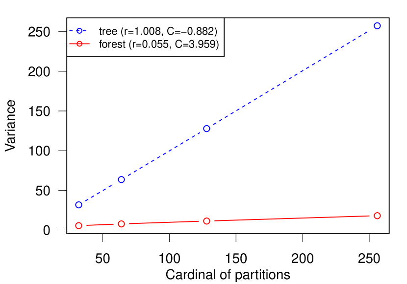
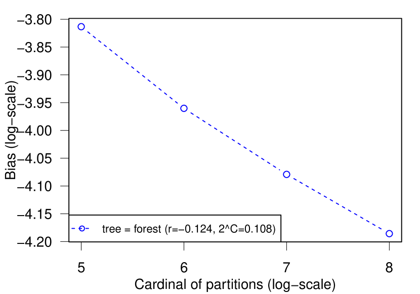
For now, we only study the behaviour of these two terms in a short numerical experiment. The results are summarized by Table 2, where estimated values of the approximation and estimation errors are reported as a function of $n_{2}$, $\sigma^{2}$ and of the parameters of the partition building process ($k$, $\mathtt{mtry}$ and bootstrap).

Table 2: Numerical estimation of the quadratic risk (approximation error + estimation error) for the hold-out random forest; $k$ is the number of cells in the partition; $\mathcal{X}=[0,1]^{p}$ with $p=5$. There is no randomization of the labels.

	Single tree	Large forest
No bootstrap $\mathtt{mtry}=p$	$\displaystyle\frac{0.13}{k^{0.17}}+\frac{1.04\sigma^{2\vphantom{{}^{2}}}k}{n_{2}}$	$\displaystyle\frac{0.13}{k^{0.17}}+\frac{1.04\sigma^{2\vphantom{{}^{2}}}k}{n_{2}}$
Bootstrap $\mathtt{mtry}=p$	$\displaystyle\frac{0.14}{k^{0.17}}+\frac{1.06\sigma^{2\vphantom{{}^{2}}}k}{n_{2}}$	$\displaystyle\frac{0.15}{k^{0.29}}+\frac{0.08\sigma^{2\vphantom{{}^{2}}}k}{n_{2}}$
No bootstrap $\mathtt{mtry}=\lfloor p/3\rfloor$	$\displaystyle\frac{0.23}{k^{0.19}}+\frac{1.01\sigma^{2\vphantom{{}^{2}}}k}{n_{2}}$	$\displaystyle\frac{0.06}{k^{0.31}}+\frac{0.06\sigma^{2\vphantom{{}^{2}}}k}{n_{2}}$
Bootstrap $\mathtt{mtry}=\lfloor p/3\rfloor$	$\displaystyle\frac{0.25}{k^{0.20}}+\frac{1.02\sigma^{2\vphantom{{}^{2}}}k}{n_{2}}$	$\displaystyle\frac{0.06}{k^{0.34}}+\frac{0.05\sigma^{2\vphantom{{}^{2}}}k}{n_{2}}$

Detailed information about this experiment can be found in Appendix C. Let us emphasize here that we consider a single data generation setting, hence these results must be interpreted with care.

2.2 Discussion

Based on Table 2 and our experience about Breiman’s random forests, we can make the following comments.

Choice of $\mathtt{mtry}$.

As illustrated in Table 2, choosing $\mathtt{mtry}=\lfloor p/3\rfloor$ instead of $p$ decreases the risk of an infinite forest. When there is no bootstrap, the performance gain is significant and the reason is that it is the only source of randomization of partitions. But, even in presence of bootstrap, it allows to slightly reduce the approximation error. In the same experiments with $p=10$, the gain of decreasing $\mathtt{mtry}$ in the bootstrap case is larger (see the supplementary material).

Our belief is that when there is some bootstrap, the additional randomization given by taking $\mathtt{mtry}<p$ can reduce the risk in some cases, where typically $n\geq p$ (which holds true in our experiments). This is supported by the experiments of Genuer et al. (2008, Section 2), where small values of mtry give significantly lower risk than $\mathtt{mtry}=p$ for some classification problems. For regression, Genuer et al. (2008, Section 2) obtain similar performance when decreasing mtry, which is consistent with Table 2 since these experiments are done in the bootstrap case.

When $n\ll p$ and only a small proportion of the coordinates of $\mathbf{x}$ are informative, we conjecture that the optimal $\mathtt{mtry}$ is close to $p$ (provided that there is some bootstrap step for randomizing the partitions). Indeed, if mtry is significantly smaller than $p$, then, the probability to choose at least one informative coordinate in $\mathcal{M}_{\mathrm{try}}$ is not close to $1$, hence the randomization of the partitions might be too strong.

Bootstrap, $\mathtt{mtry}$ and randomization of the partitions.

When $\mathtt{mtry}=p$, according to Table 2, the bootstrap helps to significantly reduce the risk, compared with the no randomization case. Overall, we get a significantly smaller risk when there is at least one source of randomization of the partitions.

Comparing the three combinations of parameters (bootstrap, $\mathtt{mtry}<p$, or both) for which the partitions are randomized is more difficult: the differences observed in Table 2 might not be significant. Nevertheless, Table 2 suggests that the lowest risk might be obtained when two sources of randomization are present ($\mathtt{mtry}<p$ and bootstrap). And if we have to choose only one source of randomization, it seems that randomizing with $\mathtt{mtry}=\lfloor p/3\rfloor$ only yields a smaller risk than bootstrapping only.

Appendix A Approximation and estimation errors

We state a general decomposition of the risk of a forest having the $X$-property (that is, when partitions are built independently from $(Y_{i})_{1\leq i\leq n}$), that we need for proving the results of Section 1, but can be useful more generally. We assume that $\mathbb{E}[Y_{i}^{2}]<+\infty$ for all $i$.

For any random forest $m_{M,n}$ having the $X$-property, following Biau and Scornet (2016, Sections 2 and 3.2), we can write

$$m_{M,n}(\mathbf{x};\Theta_{1\ldots M},\mathcal{D}_{n})=\sum_{i=1}^{n}W_{ni}(\mathbf{x})Y_{i}$$

$$\text{where}\qquad W_{ni}(\mathbf{x})=W_{ni}(\mathbf{x};\Theta_{1\ldots M},X_{1\ldots n})=\frac{1}{M}\sum_{j=1}^{M}\frac{C_{i}(\Theta_{j})\mathbf{1}_{X_{i}\in A_{n}(\mathbf{x};\Theta_{j};X_{1\ldots n})}}{N_{n}(\mathbf{x};\Theta_{j};X_{1\ldots n})}\enspace,$$ (1)

$C_{i}(\Theta_{j})$ is the number of times $(X_{i},Y_{i})$ appears in the $j$-th resample, $A_{n}(\mathbf{x};\Theta_{j};X_{1\ldots n})$ is the cell containing $\mathbf{x}$ in the $j$-th tree, and

$$N_{n}(\mathbf{x};\Theta_{j};X_{1\ldots n})=\sum_{i=1}^{n}C_{i}(\Theta_{j})\mathbf{1}_{X_{i}\in A_{n}(\mathbf{x};\Theta_{j};X_{1\ldots n})}\enspace.$$

Now, let us define

$$m^{\star}_{M,n}(\mathbf{x};\Theta_{1\ldots M},X_{1\ldots n}) =\mathbb{E}\Bigl{[}m_{M,n}(\mathbf{x};\Theta_{1\ldots M},\mathcal{D}_{n})\,\big{|}\,X_{1\ldots n},\Theta_{1\ldots M}\Bigr{]}$$

$$=\sum_{i=1}^{n}W_{ni}(\mathbf{x};\Theta_{1\ldots M},X_{1\ldots n})m(X_{i})$$

$$\text{and}\qquad\overline{m}^{\star}_{M,n}(\mathbf{x};\Theta_{1\ldots M}) =\mathbb{E}\Bigl{[}m^{\star}_{M,n}(\mathbf{x};\Theta_{1\ldots M},X_{1\ldots n})\,\big{|}\,\Theta_{1\ldots M}\Bigr{]}\enspace.$$

By definition of the conditional expectation, we can decompose the risk of $m_{M,n}$ at $\mathbf{x}$ into three terms

$$\begin{split}&\mathbb{E}\Bigl{[}\bigl{(}m_{M,n}(\mathbf{x})-m(\mathbf{x})\bigr{)}^{2}\Bigr{]}=\underbrace{\mathbb{E}\Bigl{[}\bigl{(}\overline{m}^{\star}_{M,n}(\mathbf{x})-m(\mathbf{x})\bigr{)}^{2}\Bigr{]}}_{A=\text{approximation error}}\\ \hskip 28.45274pt&+\underbrace{\mathbb{E}\Bigl{[}\bigl{(}m^{\star}_{M,n}(\mathbf{x})-\overline{m}^{\star}_{M,n}(\mathbf{x})\bigr{)}^{2}\Bigr{]}}_{\Delta}+\underbrace{\mathbb{E}\Bigl{[}\bigl{(}m_{M,n}(\mathbf{x})-m^{\star}_{M,n}(\mathbf{x})\bigr{)}^{2}\Bigr{]}}_{E=\text{estimation error}}\enspace.\end{split}$$ (2)

In the fixed-design regression setting (where the $X_{i}$ are deterministic), $A$ is called approximation error, $\Delta=0$, and $E$ is called estimation error. Things are a bit more complicated in the random-design setting—when $(X_{i},Y_{i})_{1\leq i\leq n}$ are independent and identically distributed—since $\Delta\neq 0$ in general. Up to minor differences related to how $m_{n}$ is defined on empty cells, $A$ is still the approximation error, and the estimation error is $\Delta+E$.

Let us finally assume that $(X_{i},Y_{i})_{1\leq i\leq n}$ are independent and define

$$\sigma^{2}(X_{i})=\mathbb{E}\mathopen{}\left[\bigl{(}m(X_{i})-Y_{i}\bigr{)}^{2}\,\big{|}\,X_{i}\right]\mathclose{}\enspace.$$

Then, since the weights $W_{ni}(\mathbf{x})$ only depend on $\mathcal{D}_{n}$ through $X_{1\ldots n}$, we have the following formula for the estimation error

$$E=\mathbb{E}\mathopen{}\left[\mathopen{}\left(\sum_{i=1}^{n}W_{ni}(\mathbf{x})\bigl{(}m(X_{i})-Y_{i}\bigr{)}\right)^{2}\mathclose{}\right]\mathclose{} =\mathbb{E}\mathopen{}\left[\sum_{i=1}^{n}W_{ni}(\mathbf{x})^{2}\sigma^{2}(X_{i})\right]\mathclose{}\enspace.$$

For instance, in the homoscedastic case, $\sigma^{2}(X_{i})\equiv\sigma^{2}$ and

$$E=\mathbb{E}\mathopen{}\left[\mathopen{}\left(\sum_{i=1}^{n}W_{ni}(\mathbf{x})\bigl{(}m(X_{i})-Y_{i}\bigr{)}\right)^{2}\mathclose{}\right]\mathclose{} =\sigma^{2}\mathbb{E}\mathopen{}\left[\sum_{i=1}^{n}W_{ni}(\mathbf{x})^{2}\right]\mathclose{}\enspace.$$ (3)

Appendix B Analysis of the toy forest: proofs

We prove the results stated in Section 1 for the one-dimensional toy forest.

Since the toy forest is purely random, all results of Appendix A apply, with $\Theta=(T,I)$ and $C_{i}(\Theta)=\mathbf{1}_{i\in I}$. It remains to compute the three terms of Eq. (2).

Since we assume $m$ is of class $\mathcal{C}^{3}$, we can use the results of Arlot and Genuer (2014, Section 4) for the approximation error $A$ (up to minor differences in the definition of $\overline{m}^{\star}_{M,n}(\mathbf{x})$, due to event where $A_{n}(\mathbf{x};\Theta)$ is empty, which has a small probability since $a\gg k$). We assume that $m^{\prime}(\mathbf{x})\neq 0$ and $m^{\prime\prime}(\mathbf{x})\neq 0$ for simplicity, so the quantities appearing in Table 1 indeed provide the order of magnitude of $A$.

The middle term $\Delta$ in decomposition (2) is negligible in front of $E$ for a single tree, which can be proved using results from Arlot (2008), as soon as $m^{\prime}(\mathbf{x})/k\ll\sigma$ and $a\gg k$. We assume that it can also be neglected for an infinite forest.

For the estimation error, we can use Eq. (3) and the following arguments. First, for every $i\in\{1,\ldots,n\}$, $X_{i}$ belongs to $A_{n}(\mathbf{x};\Theta)$ with probability $1/k$. Combined with the subsampling process, we get that

$$N_{n}(\mathbf{x};\Theta;X_{1\ldots n})\sim\mathcal{B}\mathopen{}\left(n,\frac{a}{nk}\right)\mathclose{}$$

is close to its expectation $a/k$ with probability almost one if $a/k\gg\log(n)$. Assuming that this holds simultaneously for a huge fraction of the subsamples, we get the approximation

$$W_{ni}^{\mathrm{toy}}(\mathbf{x}) =\frac{1}{M}\sum_{j=1}^{M}\frac{\mathbf{1}_{i\in I_{j}}\mathbf{1}_{X_{i}\in A_{n}(\mathbf{x};\Theta_{j})}}{N_{n}(\mathbf{x};\Theta_{j};X_{1\ldots n})}$$

$$\approx\frac{k}{a}\frac{1}{M}\sum_{j=1}^{M}\mathbf{1}_{i\in I_{j}}\mathbf{1}_{X_{i}\in A_{n}(\mathbf{x};\Theta_{j})}=:\widetilde{W}_{ni}^{\mathrm{toy}}(\mathbf{x})\enspace.$$ (4)

Now, we note that conditionally to $X_{1\ldots n}$, the variables $\mathbf{1}_{i\in I_{j}}\mathbf{1}_{X_{i}\in A_{n}(\mathbf{x};\Theta_{j})}$, $j=1,\ldots,M$ are independent and follow a Bernoulli distribution with the same parameter

$$\frac{a}{n}\times\bigl{(}1-k|X_{i}-x|\bigr{)}_{+}\enspace.$$

Therefore,

$$\mathbb{E}\mathopen{}\left[\widetilde{W}_{ni}^{\mathrm{toy}}(\mathbf{x})^{2}\,\big{|}\,X_{1\ldots n}\right]\mathclose{} =\frac{k^{2}}{na}\mathopen{}\left[\mathopen{}\left(1-\frac{1}{M}\right)\mathclose{}\frac{a}{n}\Bigl{(}\bigl{(}1-k|X_{i}-x|\bigr{)}_{+}\Bigr{)}^{2}+\frac{1}{M}\bigl{(}1-k|X_{i}-x|\bigr{)}_{+}\right]\mathclose{}$$

$$\text{hence}\quad\mathbb{E}\mathopen{}\left[\widetilde{W}_{ni}^{\mathrm{toy}}(\mathbf{x})^{2}\right]\mathclose{} =\frac{k}{na}\mathopen{}\left[\mathopen{}\left(1-\frac{1}{M}\right)\mathclose{}\frac{2a}{3n}+\frac{1}{M}\right]\mathclose{}\enspace.$$

By Eq. (3), this ends the proof of the results in the bottom line of Table 1.

Similar arguments apply for justifying the top line of Table 1, where $T_{j}=0$ almost surely.

Note that we have not given a full rigorous proof of the results shown in Table 1, because of the approximation (4) and of the term $\Delta$ that we have neglected. We are convinced that the parts of the proof that we have skipped might only require to add some technical assumptions, which would not help to reach our goal of understanding better random forests in general.

Appendix C Details about the experiments

This section describes the experiments whose results are shown in Section 2.

Data generation process.

We take $\mathcal{X}=[0,1]^{p}$, with $p\in\{5,10\}$. Table 2 only shows the results for $p=5$. Results for $p=10$ are shown in supplementary material.

The data $(X_{i},Y_{i})_{1\leq i\leq n_{1}+n_{2}}$ are independent with the same distribution: $X_{i}\sim\mathcal{U}([0,1]^{p})$, $Y_{i}=m(X_{i})+\varepsilon_{i}$ with $\epsilon_{i}\sim\mathcal{N}(0,\sigma^{2})$ independent from $X_{i}$, $\sigma^{2}=1/16$, and the regression function $m$ is defined by

$$m:\mathbf{x}\in[0,1]^{p}\mapsto\mathbf{1/10}\times\left[10\sin(\pi x_{1}x_{2})+20(x_{3}-0.5)^{2}+10x_{4}+5x_{5}\right]\,.$$

The function $m$ is proportional to the Friedman1 function which was introduced by Friedman (1991). Note that when $p>5$, $m$ only depends on the $5$ first coordinates of $\mathbf{x}$.

Then, the two subsamples are defined by $\mathcal{D}_{n_{1}}^{1}=(X_{i},Y_{i})_{1\leq i\leq n_{1}}$ and $\mathcal{D}_{n_{2}}^{2}=(X_{i},Y_{i})_{n_{1}+1\leq i\leq n_{1}+n_{2}}$.

We always take $n_{1}=1\,280$ and $n_{2}=25\,600$.

Trees and forests.

For each $k\in\{2^{5},2^{6},2^{7},2^{8}\}$, each experimental condition (bootstrap or not, $\mathtt{mtry}=p$ or $\lfloor p/3\rfloor$), we build some hold-out random trees and forests as defined in Section 2. These are built with the randomForest R package (Liaw and Wiener, 2002; R Core Team, 2015), with appropriate parameters ($k$ is controlled by maxnodes, while $\mathtt{nodesize}=1$).

Resampling within $\mathcal{D}_{n_{1}}^{1}$ (when there is some resampling) is done with a bootstrap sample of size $n_{1}$ (that is, with replacement and $a_{n_{1}}=n_{1}$).

“Large” forests are made of $M=k$ trees, a number of trees suggested by Arlot and Genuer (2014).

Estimates of approximation and estimation error.

Estimating approximation and estimation errors (as defined by Eq. (2)) requires to estimate some expectations over $\Theta$ (which includes the randomness of $\mathcal{D}_{n_{1}}^{1}$ as well as the randomness of the choice of bootstrap subsamples of $\mathcal{D}_{n_{1}}^{1}$ and of the repeated choices of a subset $\mathcal{M}_{\mathrm{try}}$). This is done with a Monte-Carlo approximation, with $500$ replicates for trees and $10$ replicates for forests. This number might seem small, but we observe that large forests are quite stable, hence expectations can be evaluated precisely from a small number of replicates.

We estimate the approximation error (integrated over $\mathbf{x}$) as follows. For each partition that we build, we compute the corresponding “ideal” tree, which maps each piece of the partition to the average of $m$ over it (this average can be computed almost exactly from the definition of $m$). Then, to each forest we associate the “ideal” forest $\overline{m}^{\star}_{M,n}$ which is the average of the ideal trees. We can thus compute $(\overline{m}^{\star}_{M,n}(\mathbf{x})-m(\mathbf{x}))^{2}$ for any $\mathbf{x}\in\mathcal{X}$, and estimate its expectation with respect to $\Theta$. Averaging these estimates over $1000$ uniform random points $\mathbf{x}\in\mathcal{X}$ provides our estimate of the approximation error.

We estimate the estimation error (integrated over $\mathbf{x}$) from Eq. (3); since $\sigma^{2}$ is known, we focus on the remaining term. Given some hold-out random forest, for any $\mathbf{x}\in\mathcal{X}$ and $i\in\{1,\ldots,n\}$, we can compute

$$W_{ni}(\mathbf{x})=\frac{1}{M}\sum_{j=1}^{M}\sum_{(X_{i},Y_{i})\in\mathcal{D}_{n_{2}}^{2}}\frac{\mathbf{1}_{X_{i}\in A_{n_{1}}(\mathbf{x};\Theta_{j},\mathcal{D}_{n_{1}}^{1})}}{N_{n_{2}}(\mathbf{x};\Theta_{j},\mathcal{D}_{n_{1}}^{1},\mathcal{D}_{n_{2}}^{2})}\enspace.$$

Then, averaging $\sum_{i}W_{ni}(\mathbf{x})^{2}$ over several replicate trees/forests and over $1\,000$ uniform random points $\mathbf{x}\in\mathcal{X}$, we get an estimate of the estimation error (divided by $\sigma^{2}$).

Summarizing the results in Table 2.

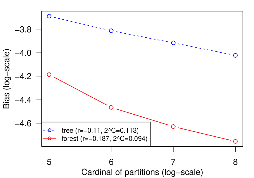
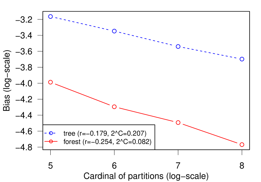
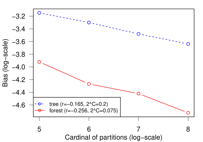
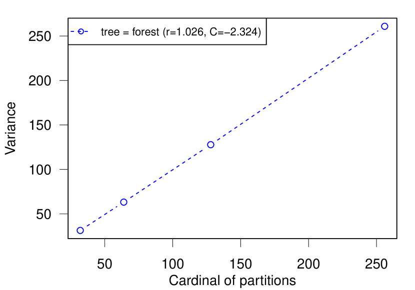
Given the estimates of the (integrated) approximation and estimation errors that we obtain for every $k\in\{2^{5},2^{6},2^{7},2^{8}\}$, we plot each kind of error as a function of $k$ (in $\mathrm{log}_{2}$-$\mathrm{log}_{2}$ scale for the approximation error), and we fit a simple linear model (with an intercept). The estimated parameters of the model directly give the results shown in Table 2 (in which the value of the intercept for the estimation error is omitted for simplicity). The corresponding graphs are shown in supplementary material.

Appendix D Supplementary Material

Table 3: Numerical estimation of the quadratic risk (approximation error + estimation error) for the hold-out random forest; $k$ is the number of cells in the partition; $\mathcal{X}=[0,1]^{p}$ with $p=10$. There is no randomization of the labels.

	Single tree	Large forest
No bootstrap $\mathtt{mtry}=p$	$\displaystyle\frac{0.11}{k^{0.12}}+\frac{1.03\sigma^{2\vphantom{{}^{2}}}k}{n_{2}}$	$\displaystyle\frac{0.11}{k^{0.12}}+\frac{1.03\sigma^{2\vphantom{{}^{2}}}k}{n_{2}}$
Bootstrap $\mathtt{mtry}=p$	$\displaystyle\frac{0.11}{k^{0.11}}+\frac{1.05\sigma^{2\vphantom{{}^{2}}}k}{n_{2}}$	$\displaystyle\frac{0.10}{k^{0.19}}+\frac{0.04\sigma^{2\vphantom{{}^{2}}}k}{n_{2}}$
No bootstrap $\mathtt{mtry}=\lfloor p/3\rfloor$	$\displaystyle\frac{0.21}{k^{0.18}}+\frac{1.08\sigma^{2\vphantom{{}^{2}}}k}{n_{2}}$	$\displaystyle\frac{0.08}{k^{0.25}}+\frac{0.04\sigma^{2\vphantom{{}^{2}}}k}{n_{2}}$
Bootstrap $\mathtt{mtry}=\lfloor p/3\rfloor$	$\displaystyle\frac{0.20}{k^{0.16}}+\frac{1.05\sigma^{2\vphantom{{}^{2}}}k}{n_{2}}$	$\displaystyle\frac{0.07}{k^{0.26}}+\frac{0.03\sigma^{2\vphantom{{}^{2}}}k}{n_{2}}$

(a) no bootstrap, $\mathtt{mtry}=5$, $p=5$

(b) bootstrap, $\mathtt{mtry}=5$, $p=5$

(c) no bootstrap, $\mathtt{mtry}=1$, $p=5$

(d) bootstrap, $\mathtt{mtry}=1$, $p=5$

Figure 1: Estimated values of the approximation error of hold-out trees and “large” forests (in $\log_{2}$-scale) as a function of the number of leaves (in $\log_{2}$-scale), for the Friedman 1 regression function in dimension $p=5$, with various values of the parameters (bootstrap or not, $\mathtt{mtry}\in\{p,\lfloor p/3\rfloor\}$). The coefficients $r$ and $C$ respectively denote the slope and the intercept of a linear model fitted to the scatter plot.

(a) no bootstrap, $\mathtt{mtry}=5$, $p=5$

(b) bootstrap, $\mathtt{mtry}=5$, $p=5$

(c) no bootstrap, $\mathtt{mtry}=1$, $p=5$

(d) bootstrap, $\mathtt{mtry}=1$, $p=5$

Figure 2: Estimated values of the estimation error (multiplied by $n_{2}/\sigma^{2}$) of hold-out trees and “large” forests as a function of the number of leaves, for the Friedman 1 regression function in dimension $p=5$, with various values of the parameters (bootstrap or not, $\mathtt{mtry}\in\{p,\lfloor p/3\rfloor\}$). The coefficients $r$ and $C$ respectively denote the slope and the intercept of a linear model fitted to the scatter plot.

(a) no bootstrap, $\mathtt{mtry}=10$, $p=10$

(b) bootstrap, $\mathtt{mtry}=10$, $p=10$

(c) no bootstrap, $\mathtt{mtry}=3$, $p=10$

(d) bootstrap, $\mathtt{mtry}=3$, $p=10$

Figure 3: Estimated values of the approximation error of hold-out trees and “large” forests (in $\log_{2}$-scale) as a function of the number of leaves (in $\log_{2}$-scale), for the Friedman 1 regression function in dimension $p=10$, with various values of the parameters (bootstrap or not, $\mathtt{mtry}\in\{p,\lfloor p/3\rfloor\}$). The coefficients $r$ and $C$ respectively denote the slope and the intercept of a linear model fitted to the scatter plot.

(a) no bootstrap, $\mathtt{mtry}=10$, $p=10$

(b) bootstrap, $\mathtt{mtry}=10$, $p=10$

(c) no bootstrap, $\mathtt{mtry}=3$, $p=10$

(d) bootstrap, $\mathtt{mtry}=3$, $p=10$

Figure 4: Estimated values of the estimation error (multiplied by $n_{2}/\sigma^{2}$) of hold-out trees and “large” forests as a function of the number of leaves, for the Friedman 1 regression function in dimension $p=10$, with various values of the parameters (bootstrap or not, $\mathtt{mtry}\in\{p,\lfloor p/3\rfloor\}$). The coefficients $r$ and $C$ respectively denote the slope and the intercept of a linear model fitted to the scatter plot.

References

• Arlot (2008) Sylvain Arlot. V𝑉V-fold cross-validation improved: V𝑉V-fold penalization, February 2008. arXiv:0802.0566v2.
• Arlot and Genuer (2014) Sylvain Arlot and Robin Genuer. Analysis of purely random forests bias, July 2014. arXiv:1407.3939v1.
• Biau (2012) Gérard Biau. Analysis of a random forests model. J. Mach. Learn. Res., 13:1063–1095, 2012. ISSN 1532-4435.
• Biau and Scornet (2016) Gérard Biau and Erwan Scornet. A random forest guided tour. TEST, 2016. To appear.
• Bühlmann and Yu (2002) Peter Bühlmann and Bin Yu. Analyzing bagging. Ann. Statist., 30(4):927–961, 2002. ISSN 0090-5364.
• Friedman (1991) Jerome H Friedman. Multivariate adaptive regression splines. The annals of statistics, pages 1–67, 1991.
• Genuer (2012) Robin Genuer. Variance reduction in purely random forests. Journal of Nonparametric Statistics, 24(3):543–562, 2012.
• Genuer et al. (2008) Robin Genuer, Jean-Michel Poggi, and Christine Tuleau. Random forests: some methodological insights, 2008. arXiv:0811.3619.
• Liaw and Wiener (2002) Andy Liaw and Matthew Wiener. Classification and regression by randomforest. R News, 2(3):18–22, 2002. URL http://CRAN.R-project.org/doc/Rnews/.
• R Core Team (2015) R Core Team. R: A Language and Environment for Statistical Computing. R Foundation for Statistical Computing, Vienna, Austria, 2015. URL http://www.R-project.org/.