Learning A Deep $\ell_{\infty}$ Encoder for Hashing

Abstract

We investigate the $\ell_{\infty}$-constrained representation which demonstrates robustness to quantization errors, utilizing the tool of deep learning. Based on the Alternating Direction Method of Multipliers (ADMM), we formulate the original convex minimization problem as a feed-forward neural network, named Deep $\ell_{\infty}$ Encoder, by introducing the novel Bounded Linear Unit (BLU) neuron and modeling the Lagrange multipliers as network biases. Such a structural prior acts as an effective network regularization, and facilitates the model initialization. We then investigate the effective use of the proposed model in the application of hashing, by coupling the proposed encoders under a supervised pairwise loss, to develop a Deep Siamese $\ell_{\infty}$ Network, which can be optimized from end to end. Extensive experiments demonstrate the impressive performances of the proposed model. We also provide an in-depth analysis of its behaviors against the competitors.

1 Introduction

1.1 Problem Definition and Background

While $\ell_{0}$ and $\ell_{1}$ regularizations have been well-known and successfully applied in sparse signal approximations, it has been less explored to utilize the $\ell_{\infty}$ norm to regularize signal representations. In this paper, we are particularly interested in the following $\ell_{\infty}$-constrained least squares problem:

$$\begin{array}[]{l}\min_{x}||\mathbf{D}x-y||_{2}^{2}\quad s.t.\quad||x||_{\infty}\leq\lambda,\end{array}$$ (1)

where $y\in R^{n\times 1}$ denotes the input signal, $\mathbf{D}\in R^{n\times N}$ the (overcomplete) the basis (often called frame or dictionary) with $N<n$, and $x\in R^{N\times 1}$ the learned representation. Further, the maximum absolute magnitude of $x$ is bounded by a positive constant $\lambda$, so that each entry of $x$ has the smallest dynamic range Lyubarskii and Vershynin (2010). As a result, The model (1) tends to spread the information of $y$ approximately evenly among the coefficients of $x$. Thus, $x$ is called “democratic” Studer et al. (2014) or “anti-sparse” Fuchs (2011), as all of its entries are of approximately the same importance.

In practice, $x$ usually has most entries reaching the same absolute maximum magnitude Studer et al. (2014), therefore resembling to an antipodal signal in an $N$-dimensional Hamming space. Furthermore, the solution $x$ to (1) withstands errors in a very powerful way: the representation error gets bounded by the average, rather than the sum, of the errors in the coefficients. These errors may be of arbitrary nature, including distortion (e.g., quantization) and losses (e.g., transmission failure). This property was quantitatively established in Section II.C of Lyubarskii and Vershynin (2010):

Theorem 1.1.

Assume $||x||_{2}<1$ without loss of generality, and each coefficient of $x$ is quantized separately by performing a uniform scalar quantization of the dynamic range [$-\lambda,\lambda$] with $L$ levels. The overall quantization error of $x$ from (1) is bounded by $\frac{\lambda\sqrt{N}}{L}$. In comparision, a least squares solution $x_{LS}$, by minimizing $||\mathbf{D}x_{LS}-y||_{2}^{2}$ without any constraint, would only give the bound $\frac{\sqrt{n}}{L}$.

In the case of $N<<n$, the above will yield great robustness for the solution to (1) with respect to noise, in particular quantization errors. Also note that its error bound will not grow with the input dimensionality $n$, a highly desirable stability property for high-dimensional data. Therefore, (1) appears to be favorable for the applications such as vector quantization, hashing and approximate nearest neighbor search.

In this paper, we investigate (1) in the context of deep learning. Based on the Alternating Direction Methods of Multipliers (ADMM) algorithm, we formulate (1) as a feed-forward neural network Gregor and LeCun (2010), called Deep $\ell_{\infty}$ Encoder, by introducing the novel Bounded Linear Unit (BLU) neuron and modeling the Lagrange multipliers as network biases. The major technical merit to be presented, is how a specific optimization model (1) could be translated to designing a task-specific deep model, which displays the desired quantization-robust property. We then study its application in hashing, by developing a Deep Siamese $\ell_{\infty}$ Network that couples the proposed encoders under a supervised pairwise loss, which could be optimized from end to end. Impressive performances are observed in our experiments.

1.2 Related Work

Similar to the case of $\ell_{0}$/$\ell_{1}$ sparse approximation problems, solving (1) and its variants (e.g., Studer et al. (2014)) relies on iterative solutions. Stark and Parker (1995) proposed an active set strategy similar to that of Lawson and Hanson (1974). In Adlers (1998), the authors investigated a primal-dual path-following interior-point method. Albeit effective, the iterative approximation algorithms suffer from their inherently sequential structures, as well as the data-dependent complexity and latency, which often constitute a major bottleneck in the computational efficiency. In addition, the joint optimization of the (unsupervised) feature learning and the supervised steps has to rely on solving complex bi-level optimization problems Wang et al. (2015). Further, to effectively represent datasets of growing sizes, a larger dictionaries $\mathbf{D}$ is usually in need. Since the inference complexity of those iterative algorithms increases more than linearly with respect to the dictionary size Bertsekas (1999), their scalability turns out to be limited. Last but not least, while the hyperparameter $\lambda$ sometimes has physical interpretations, e.g., for signal quantization and compression, it remains unclear how to be set or adjusted for many application cases.

Deep learning has recently attracted great attentions Krizhevsky et al. (2012). The advantages of deep learning lie in its composition of multiple non-linear transformations to yield more abstract and descriptive embedding representations. The feed-forward networks could be naturally tuned jointly with task-driven loss functions Wang et al. (2016c). With the aid of gradient descent, it also scales linearly in time and space with the number of train samples.

There has been a blooming interest in bridging “shallow” optimization and deep learning models. In Gregor and LeCun (2010), a feed-forward neural network, named LISTA, was proposed to efficiently approximate the sparse codes, whose hyperparameters were learned from general regression. In Sprechmann et al. (2013), the authors leveraged a similar idea on fast trainable regressors and constructed feed-forward network approximations of the learned sparse models. It was later extended in Sprechmann et al. (2015) to develop a principled process of learned deterministic fixed-complexity pursuits, for sparse and low rank models. Lately, Wang et al. (2016c) proposed Deep $\ell_{0}$ Encoders, to model $\ell_{0}$ sparse approximation as feed-forward neural networks. The authors extended the strategy to the graph-regularized $\ell_{1}$ approximation in Wang et al. (2016b), and the dual sparsity model in Wang et al. (2016a). Despite the above progress, up to our best knowledge, few efforts have been made beyond sparse approximation (e.g., $\ell_{0}$/$\ell_{1}$) models.

2 An ADMM Algorithm

ADMM has been popular for its remarkable effectiveness in minimizing objectives with linearly separable structures Bertsekas (1999). We first introduce an auxiliary variable $z\in R^{N\times 1}$, and rewrite (1) as:

$$\begin{array}[]{l}\min_{\mathbf{x,z}}\frac{1}{2}||\mathbf{D}x-y||_{2}^{2}\quad s.t.\quad||z||_{\infty}\leq\lambda,\quad z-x=0.\end{array}$$ (2)

The augmented Lagrangian function of (2) is:

$$\begin{array}[]{l}\frac{1}{2}||\mathbf{D}x-y||_{2}^{2}+p^{T}(z-x)+\frac{\beta}{2}||z-x||^{2}_{2}+\Phi_{\lambda}(z).\end{array}$$ (3)

Here $p\in R^{N\times 1}$ is the Lagrange multiplier attached to the equality constraint, $\beta$ is a positive constant (with a default value 0.6), and $\Phi_{\lambda}(z)$ is the indicator function which goes to infinity when $||z||_{\infty}>\lambda$ and 0 otherwise. ADMM minimizes (3) with respect to $x$ and $z$ in an alternating direction manner, and updates $p$ accordingly. It guarantees global convergence to the optimal solution to (1). Starting from any initialization points of $x$, $z$, and $p$, ADMM iteratively solves ($t$ = 0, 1, 2… denotes the iteration number):

$$\begin{array}[]{l}\text{{x update:}}\quad\min_{x_{t+1}}\frac{1}{2}||\mathbf{D}x-y||_{2}^{2}-p_{t}^{T}x+\frac{\beta}{2}||z_{t}-x||^{2}_{2},\end{array}$$ (4)

$$\begin{array}[]{l}\text{{z update:}}\quad\min_{z_{t+1}}\frac{\beta}{2}||z-(x_{t+1}-\frac{p_{t}}{\beta})||^{2}_{2}+\Phi_{\lambda}(z),\end{array}$$ (5)

$$\begin{array}[]{l}\text{{p update:}}\quad p_{t+1}=p_{t}+\beta(z_{t+1}-x_{t+1}).\end{array}$$ (6)

Furthermore, both (4) and (5) enjoy closed-form solutions:

$$\begin{array}[]{l}x_{t+1}=(\mathbf{D}^{T}\mathbf{D}+\beta\mathbf{I})^{-1}(\mathbf{D}^{T}y+\beta z_{t}+p_{t}),\end{array}$$ (7)

$$\begin{array}[]{l}z_{t+1}=\min(\max(x_{t+1}-\frac{p_{t}}{\beta},-\lambda),\lambda).\end{array}$$ (8)

The above algorithm could be categorized to the primal-dual scheme. However, discussing the ADMM algorithm in more details is beyond the focus of this paper. Instead, the purpose of deriving (2)-(8) is to preparing us for the design of the task-specific deep architecture, as presented below.

3 Deep $\ell_{\infty}$ Encoder

We first substitute (7) into (8), in order to derive an update form explicitly dependent on only $z$ and $p$:

$$\begin{array}[]{l}z_{t+1}=B_{\lambda}((\mathbf{D}^{T}\mathbf{D}+\beta\mathbf{I})^{-1}(\mathbf{D}^{T}y+\beta z_{t}+p_{t})-\frac{p_{t}}{\beta}),\end{array}$$ (9)

where $B_{\lambda}$ is defined as a box-constrained element-wise operator ($u$ denotes a vector and $u_{i}$ is its $i$-th element):

$$[B_{\lambda}(u)]_{i}=\min(\max(u_{i},-\lambda),\lambda).$$ (10)

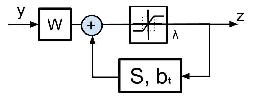
Figure 1: The block diagram of solving solving (1).

.

Figure 2: Deep $\ell_{\infty}$ Encoder, with two time-unfolded stages.

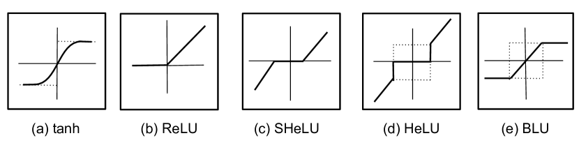
Figure 3: A comparison among existing neurons and BLU.

Eqn. (9) could be alternatively rewritten as:

$$\begin{array}[]{l}\mathbf{z}_{t+1}=B_{\lambda}(\mathbf{W}y+\mathbf{S}z_{t}+b_{t}),$ $\text{where:}\\ \mathbf{W}=(\mathbf{D}^{T}\mathbf{D}+\beta\mathbf{I})^{-1}\mathbf{D}^{T},\mathbf{S}=\beta(\mathbf{D}^{T}\mathbf{D}+\beta\mathbf{I})^{-1},\\ b_{t}=[(\mathbf{D}^{T}\mathbf{D}+\beta\mathbf{I})^{-1}-\frac{1}{\beta}\mathbf{I}]p_{t},\end{array}$$ (11)

and expressed as the block diagram in Fig. 1, which outlines a recurrent structure of solving (1). Note that in (11), while $\mathbf{W}$ and $\mathbf{S}$ are pre-computed hyperparamters shared across iterations, $b_{t}$ remains to be a variable dependent on $p_{t}$, and has to be updated throughout iterations too ($b_{t}$’s update block is omitted in Fig. 1).

By time-unfolding and truncating Fig. 1 to a fixed number of $K$ iterations ($K$ = 2 by default), we obtain a feed-forward network structure in Fig. 2, named Deep $\ell_{\infty}$ Encoder. Since the threshold $\lambda$ is less straightforward to update, we repeat the same trick in Wang et al. (2016c) to rewrite (10) as: $[B_{\lambda}(u)]_{i}=\lambda_{i}B_{1}(u_{i}/\lambda_{i})$. The original operator is thus decomposed into two linear diagonal scaling layers, plus a unit-threshold neuron, the latter of which is called a Bounded Linear Unit (BLU) by us. All the hyperparameters $\mathbf{W}$, $\mathbf{S}_{k}$ and $b_{k}$ ($k$ = 1, 2), as well as $\lambda$, are all to be learnt from data by back-propogation. Although the equations in (11) do not directly apply to solving the deep $\ell_{\infty}$ encoder, they can serve as high-quality initializations.

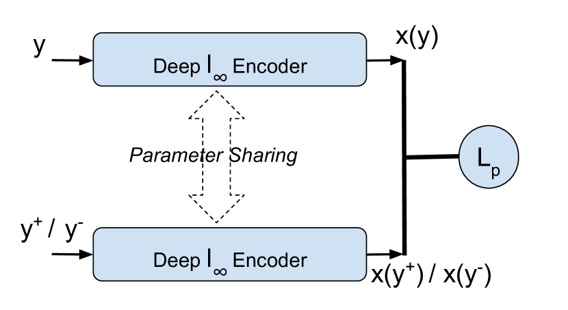
Figure 4: Deep $\ell_{\infty}$ Siamese Network, by coupling two parameter-sharing encoders, followed by a pairwise loss (12).

It is crucial to notice the modeling of the Lagrange multipliers $p_{t}$ as the biases, and to incorporate its updates into network learning. That provides important clues on how to relate deep networks to a larger class of optimization models, whose solutions rely on dual domain methods.

Comparing BLU with existing neurons As shown in Fig. 3 (e), BLU tends to suppress large entries while not penalizing small ones, resulting in dense, nearly antipodal representations. A first look at the plot of BLU easily reminds the tanh neuron (Fig. 3 (a)). In fact, with the its output range $[-1,1]$ and a slope of 1 at the origin, tanh could be viewed as a smoothened differentiable approximation of BLU.

We further compare BLU with other popular and recently proposed neurons: Rectifier Linear Unit (ReLU) Krizhevsky et al. (2012), Soft-tHresholding Linear Unit (SHeLU) Wang et al. (2016b), and Hard thrEsholding Linear Unit (HELU) Wang et al. (2016c), as depicted in Fig. 3 (b)-(d), respectively. Contrary to BLU and tanh, they all introduce sparsity in the outputs, and thus prove successful and outperform tanh in classification and recognition tasks. Interestingly, HELU seems exactly the rival against BLU, as it does not penalize large entries but suppresses small ones down to zero.

4 Deep $\ell_{\infty}$ Siamese Network for Hashing

Rather than solving (1) first and then training the encoder as general regression, as Gregor and LeCun (2010) did, we instead concatenate encoder(s) with a task-driven loss, and optimize the pipeline from end to end. In this paper, we focus on discussing its application in hashing, although the proposed model is not limited to one specific application.

Background With the ever-growing large-scale image data on the Web, much attention has been devoted to nearest neighbor search via hashing methods Gionis et al. (1999). For big data applications, compact bitwise representations improve the efficiency in both storage and search speed. The state-of-the-art approach, learning-based hashing, learns similarity-preserving hash functions to encode input data into binary codes. Furthermore, while earlier methods, such as linear search hashing (LSH) Gionis et al. (1999), iterative quantization (ITQ) Gong and Lazebnik (2011) and spectral hashing (SH) Weiss et al. (2009), do not refer to any supervised information, it has been lately discovered that involving the data similarities/dissimilarities in training benefits the performance Kulis and Darrell (2009); Liu et al. (2012).

Prior Work Traditional hashing pipelines first represent each input image as a (hand-crafted) visual descriptor, followed by separate projection and quantization steps to encode it into a binary code. Masci et al. (2014) first applied the siamese network Hadsell et al. (2006) architecture to hashing, which fed two input patterns into two parameter-sharing “encoder” columns and minimized a pairwise-similarity/dissimilarity loss function between their outputs, using pairwise labels. The authors further enforced the sparsity prior on the hash codes in Masci et al. (2013), by substituting a pair of LISTA-type encoders Gregor and LeCun (2010) for the pair of generic feed-forward encoders in Masci et al. (2014) Xia et al. (2014); Li et al. (2015) utilized tailored convolution networks with the aid of pairwise labels. Lai et al. (2015) further introduced a triplet loss with a divide-and-encode strategy applied to reduce the hash code redundancy. Note that for the final training step of quantization, Masci et al. (2013) relied on an extra hidden layer of tanh neurons to approximate binary codes, while Lai et al. (2015) exploited a piece-wise linear and discontinuous threshold function.

Our Approach In view of its robustness to quantization noise, as well as BLU’s property as a natural binarization approximation, we construct a siamese network as in Masci et al. (2014), and adopt a pair of parameter-sharing deep $\ell_{\infty}$ encoders as the two columns. The resulting architecture, named the Deep $\ell_{\infty}$ Siamese Network, is illustrated in Fig. 4. Assume $y$ and $y^{+}$ make a similar pair while $y$ and $y^{-}$ make a dissimilar pair, and further denote $x(y)$ the output representation by inputting $y$. The two coupled encoders are then optimized under the following pairwise loss (the constant $m$ represents the margin between dissimilar pairs):

$$\begin{array}[]{l}L_{p}:=\frac{1}{2}||x(y)-x(y^{+})||^{2}-\\ \frac{1}{2}(\max(0,m-||x(y)-x(y^{-})||))^{2}.\end{array}$$ (12)

The representation is learned to make similar pairs as close as possible and dissimilar pairs at least at distance $m$. In this paper, we follow Masci et al. (2014) to use a default $m$ = 5 for all experiments.

Once a deep $\ell_{\infty}$ siamese network is learned, we apply its encoder part (i.e., a deep $\ell_{\infty}$ encoder) to a new input. The computation is extremely efficient, involving only a few matrix multiplications and element-wise thresholding operations, with a total complexity of $O(nN+2N^{2})$. One can obtain a $N$-bit binary code by simply quantizing the output.

Table 1: Comparison of NNH, SNNH, and the proposed deep $\ell_{\infty}$ siamese network.

	encoder	neuron	structural prior
	type	type	on hashing codes
NNH	generic	tanh	/
SNNH	LISTA	SHeLU	sparse
Proposed	deep $\ell_{\infty}$	BLU	nearly antipodal
			& quantization-robust

5 Experiments in Image Hashing

Implementation The proposed networks are implemented with the CUDA ConvNet package Krizhevsky et al. (2012). We use a constant learning rate of 0.01 with no momentum, and a batch size of 128. Different from prior findings such as in Wang et al. (2016c, b), we discover that untying the values of $\mathbf{S}_{1}$, $b_{1}$ and $\mathbf{S}_{2}$, $b_{2}$ boosts the performance more than sharing them. It is not only because that more free parameters enable a larger learning capacity, but also due to the important fact that $p_{t}$ (and thus $b_{k}$) is in essence not shared across iterations, as in (11) and Fig. 2.

While many neural networks are trained well with random initializations, it has been discovered that sometimes poor initializations can still hamper the effectiveness of first-order methods Sutskever et al. (2013). On the other hand, It is much easier to initialize our proposed models in the right regime. We first estimate the dictionary $\mathbf{D}$ using the standard K-SVD algorithm Elad and Aharon (2006), and then inexactly solve (1) for up to $K$ ($K$ = 2) iterations, via the ADMM algorithm in Section 2, with the values of Lagrange multiplier $p_{t}$ recorded for each iteration. Benefiting from the analytical correspondence relationships in (11), it is then straightforward to obtain high-quality initializations for $\mathbf{W}$, $\mathbf{S}_{k}$ and $b_{k}$ ($k$ = 1, 2). As a result, we could achieve a steadily decreasing curve of training errors, without performing common tricks such as annealing the learning rate, which are found to be indispensable if random initialization is applied.

Table 2: Performance (%) of different hashing methods on the CIFAR10 dataset, with different code lengths $N$.

						Hamming radius $\leq 2$			Hamming radius $=0$
Method					mAP	Prec.	Recall	F1	Prec.	Recall	F1
				$N$
KSH				48	31.10	18.22	0.86	1.64	5.39	5.6$\times 10^{-2}$	0.11
				64	32.49	10.86	0.13	0.26	2.49	9.6$\times 10^{-3}$	1.9$\times 10^{-2}$
AGH1				48	14.55	15.95	2.8$\times 10^{-2}$	5.6$\times 10^{-2}$	4.88	2.2$\times 10^{-3}$	4.4$\times 10^{-3}$
				64	14.22	6.50	4.1$\times 10^{-3}$	8.1$\times 10^{-3}$	3.06	1.2$\times 10^{-3}$	2.4$\times 10^{-3}$
AGH2				48	15.34	17.43	7.1$\times 10^{-2}$	3.6$\times 10^{-2}$	5.44	3.5$\times 10^{-3}$	6.9$\times 10^{-3}$
				64	14.99	7.63	7.2$\times 10^{-3}$	1.4$\times 10^{-2}$	3.61	1.4$\times 10^{-3}$	2.7$\times 10^{-3}$
PSH				48	15.78	9.92	6.6$\times 10^{-3}$	1.3$\times 10^{-2}$	0.30	5.1$\times 10^{-5}$	1.0$\times 10^{-4}$
				64	17.18	1.52	3.0$\times 10^{-4}$	6.1$\times 10^{-4}$	1.0$\times 10^{-3}$	1.69$\times 10^{-5}$	3.3$\times 10^{-5}$
LH				48	13.13	3.0$\times 10^{-3}$	1.0$\times 10^{-4}$	5.1$\times 10^{-5}$	1.0$\times 10^{-3}$	1.7$\times 10^{-5}$	3.4$\times 10^{-5}$
				64	13.07	1.0$\times 10^{-3}$	1.7$\times 10^{-5}$	3.3$\times 10^{-5}$	0.00	0.00	0.00
NNH				48	31.21	34.87	1.81	3.44	10.02	9.4$\times 10^{-2}$	0.19
				64	35.24	23.23	0.29	0.57	5.89	1.4$\times 10^{-2}$	2.8$\times 10^{-2}$
SNNH				48	26.67	32.03	12.10	17.56	19.95	0.96	1.83
				64	27.25	30.01	36.68	33.01	30.25	9.8	14.90
Proposed				48	31.48	36.89	12.47	18.41	24.82	0.94	1.82
				64	36.76	38.67	30.28	33.96	33.30	8.9	14.05

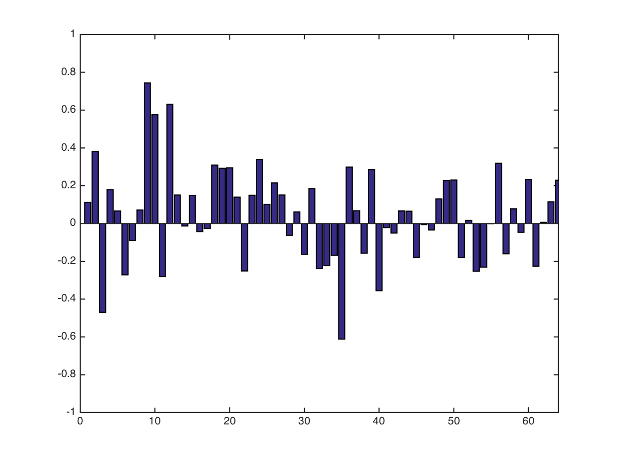
(a) NNH representation

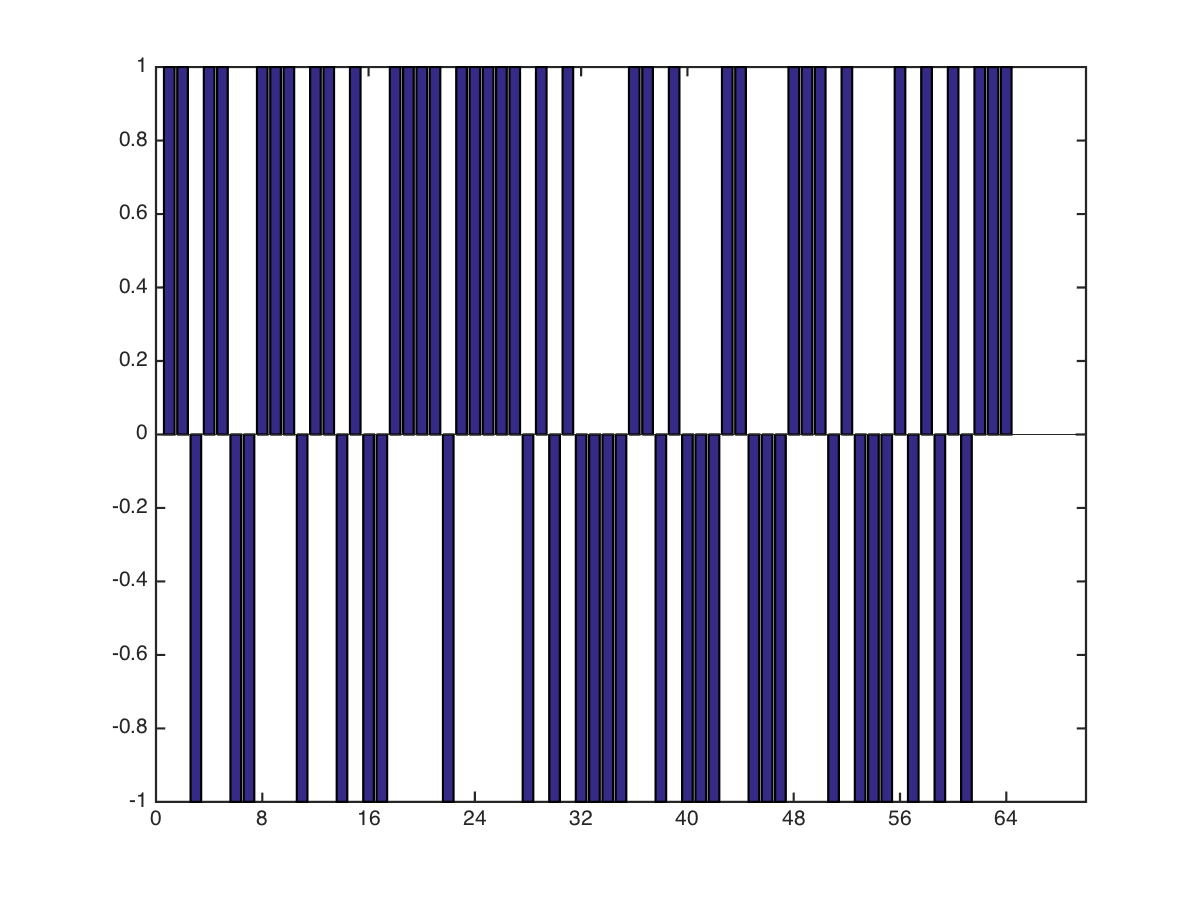
(b) NNH binary hashing code

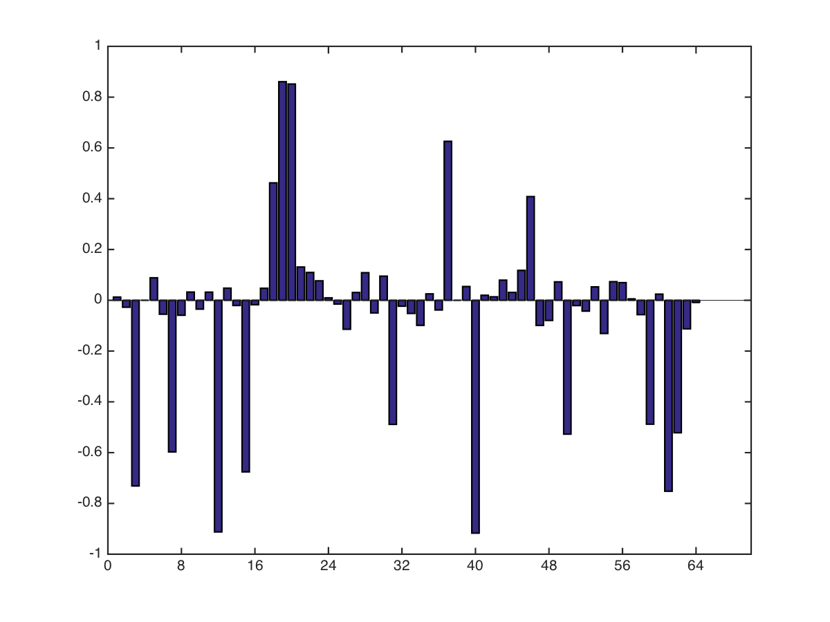
(c) SNNH representation

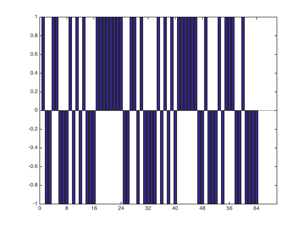
(d) SNNH binary hashing code

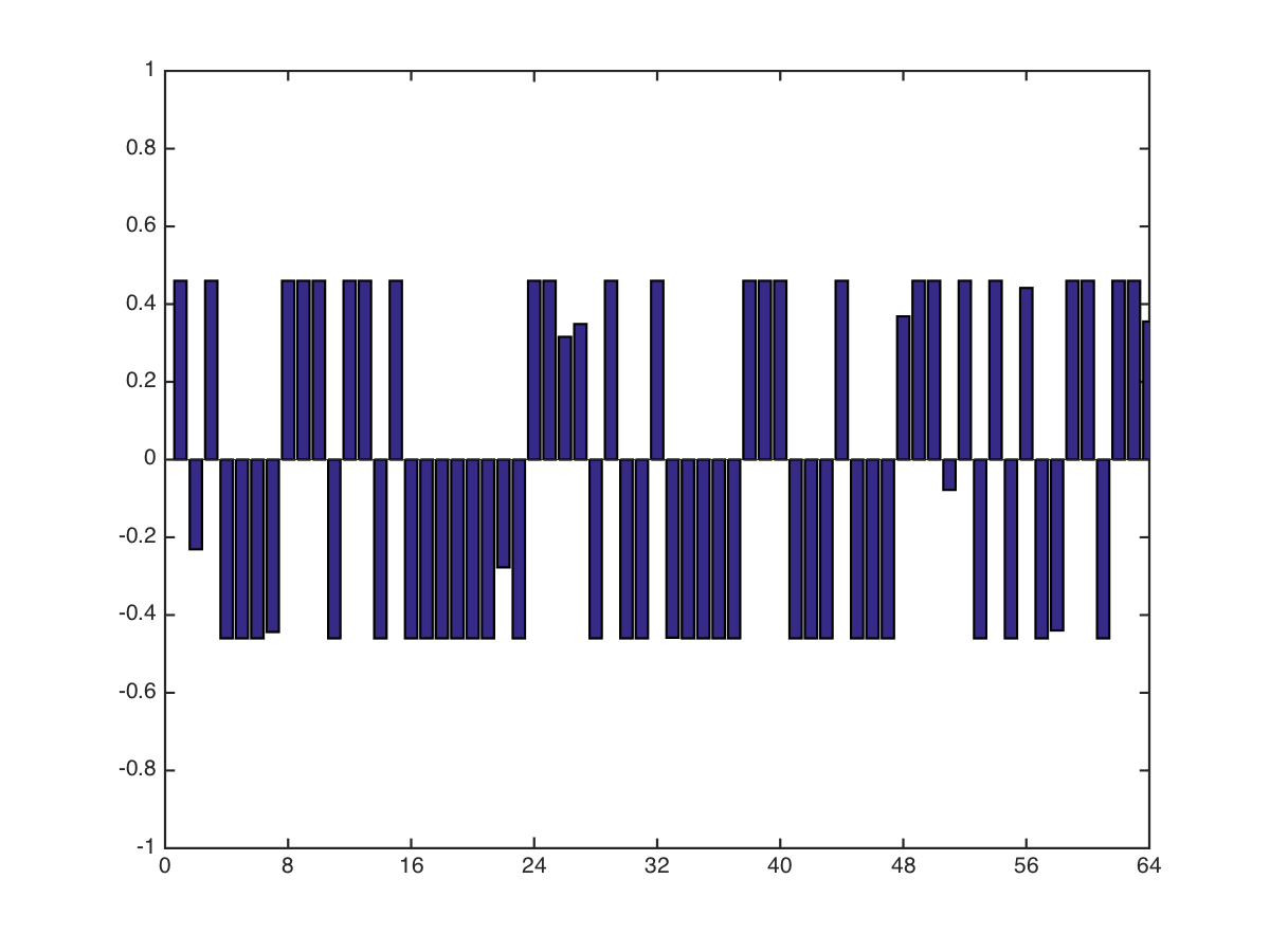
(e) Deep $\ell_{\infty}$ representation

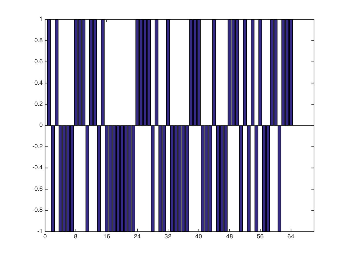
(f) Deep $\ell_{\infty}$ binary hashing code

Figure 5: The learned representations and binary hashing codes of one test image from CIFAR10, through: (a) (b) NNH; (c) (d) SNNH; (e) (f) proposed.

Datasets The CIFAR10 dataset Krizhevsky and Hinton (2009) contains 60K labeled images of 10 different classes. The images are represented using 384-dimensional GIST descriptors Oliva and Torralba (2001). Following the classical setting in Masci et al. (2013), we used a training set of 200 images for each class, and a disjoint query set of 100 images per class. The remaining 59K images are treated as database.

NUS-WIDE Chua et al. (2009) is a dataset containing 270K annotated images from Flickr. Every images is associated with one or more of the different 81 concepts, and is described using a 500-dimensional bag-of-features. In training and evaluation, we followed the protocol of Liu et al. (2011): two images were considered as neighbors if they share at least one common concept (only 21 most frequent concepts are considered). We use 100K pairs of images for training, and a query set of 100 images per concept in testing.

Comparison Methods We compare the proposed deep $\ell_{\infty}$ siamese network to six state-of-the-art hashing methods:

• four representative “shallow” hashing methods: kernelized supervised hashing (KSH) Liu et al. (2012), anchor graph hashing (AGH) Liu et al. (2011) (we compare with its two alternative forms: AGH1 and AGH2; see the original paper), parameter-sensitive hashing (PSH) Shakhnarovich et al. (2003), and LDA Hash (LH) Strecha et al. (2012) .

• two latest “deep” hashing methods: neural-network hashing (NNH) Masci et al. (2014), and sparse neural-network hashing (SNNH) Masci et al. (2013).

Comparing the two “deep” competitors to the deep $\ell_{\infty}$ siamese network, the only difference among the three is the type of encoder adopted in each’s twin columns, as listed in Table 1. We re-implement the encoder parts of NNH and SNNH, with three hidden layers (i.e, two unfolded stages for LISTA), so that all three deep hashing models have the same depth. Recall that the input $y\in R^{n}$ and the hash code $x\in R^{N}$, we immediately see from (11) that $\mathbf{W}\in R^{n\times N}$, $\mathbf{S}_{k}\in R^{N\times N}$, and $b_{k}\in R^{N}$. We carefully ensure that both NNHash and SparseHash have all their weight layers of the same dimensionality with ours, for a fair comparison.

Table 3: Performance (%) of different hashing methods on the NUS-WIDE dataset, with different code lengths $N$.

							Hamming radius $\leq 2$			Hamming radius $=0$
Method					mAP@10	MP@5K	Prec.	Recall	F1	Prec.	Recall	F1
				$N$
KSH				64	72.85	42.74	83.80	6.1$\times 10^{-3}$	1.2$\times 10^{-2}$	84.21	1.7$\times 10^{-3}$	3.3$\times 10^{-3}$
				256	73.73	45.35	84.24	1.4$\times 10^{-3}$	2.9$\times 10^{-3}$	84.24	1.4$\times 10^{-3}$	2.9$\times 10^{-3}$
AGH1				64	69.48	47.28	69.43	0.11	0.22	73.35	3.9$\times 10^{-2}$	7.9$\times 10^{-2}$
				256	73.86	46.68	75.90	1.5$\times 10^{-2}$	2.9$\times 10^{-2}$	81.64	3.6$\times 10^{-3}$	7.1$\times 10^{-3}$
AGH2				64	68.90	47.27	68.73	0.14	0.28	72.82	5.2$\times 10^{-2}$	0.10
				256	73.00	47.65	74.90	5.3$\times 10^{-2}$	0.11	80.45	1.1$\times 10^{-2}$	2.2$\times 10^{-2}$
PSH				64	72.17	44.79	60.06	0.12	0.24	81.73	1.1$\times 10^{-2}$	2.2$\times 10^{-2}$
				256	73.52	47.13	84.18	1.8$\times 10^{-3}$	3.5$\times 10^{-3}$	84.24	1.5$\times 10^{-3}$	2.9$\times 10^{-3}$
LH				64	71.33	41.69	84.26	1.4$\times 10^{-3}$	2.9$\times 10^{-3}$	84.24	1.4$\times 10^{-3}$	2.9$\times 10^{-3}$
				256	70.73	39.02	84.24	1.4$\times 10^{-3}$	2.9$\times 10^{-3}$	84.24	1.4$\times 10^{-3}$	2.9$\times 10^{-3}$
NNH				64	76.39	59.76	75.51	1.59	3.11	81.24	0.10	0.20
				256	78.31	61.21	83.46	5.8$\times 10^{-2}$	0.11	83.94	4.9$\times 10^{-3}$	9.8$\times 10^{-3}$
SNNH				64	74.87	56.82	72.32	1.99	3.87	81.98	0.37	0.73
				256	74.73	59.37	80.98	0.10	0.19	82.85	0.98	1.94
Proposed				64	79.89	63.04	79.95	1.72	3.38	86.23	0.30	0.60
				256	80.02	65.62	84.63	7.2$\times 10^{-2}$	0.15	89.49	0.57	1.13

We adopt the following classical criteria for evaluation: 1) precision and recall (PR) for different Hamming radii, and the F1 score as their harmonic average; 2) mean average precision (MAP) Müller et al. (2001). Besides, for NUS-WIDE, as computing mAP is slow over this large dataset, we follow the convention of Masci et al. (2013) to compute the mean precision (MP) of top-5K returned neighbors (MP@5K), as well as report mAP of top-10 results (mAP@10).

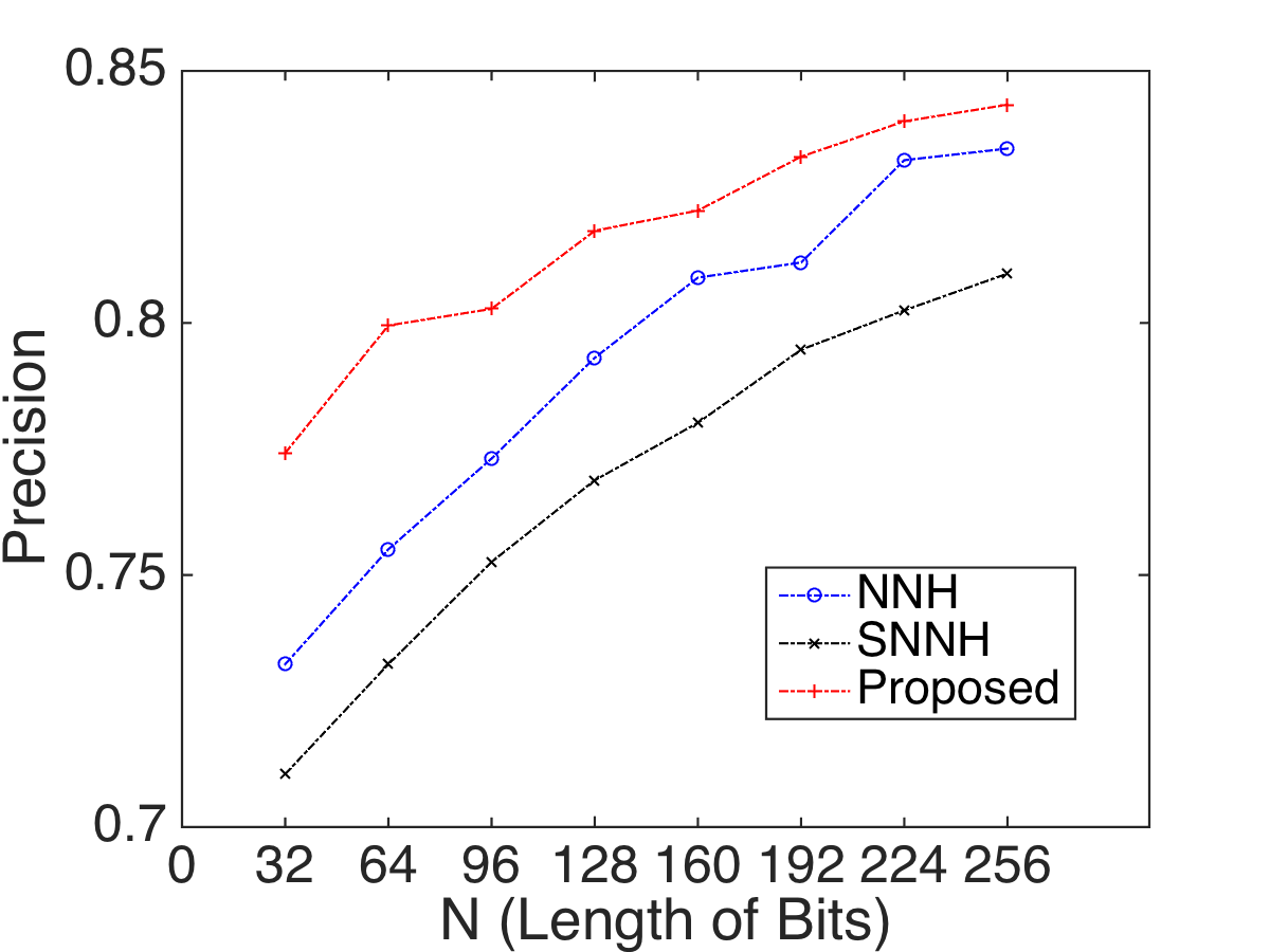
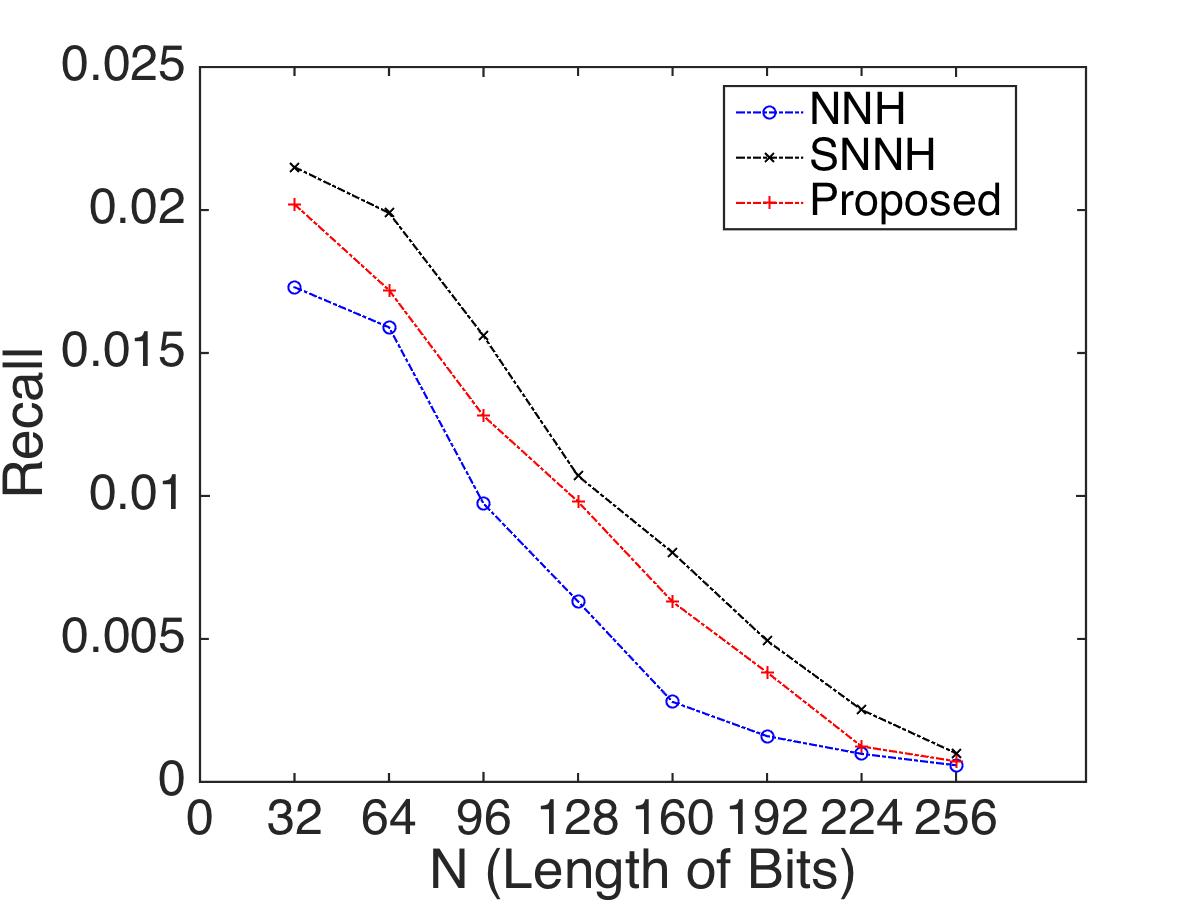
Figure 6: The comparison of three deep hashing methods on NUS-WIDE: (a) precision curve; (b) recall curve, both w.r.t the hashing code length $N$, within the Hamming radius of 2.

We have not compared with convolutional network-based hashing methods Xia et al. (2014); Li et al. (2015); Lai et al. (2015), since it is difficult to ensure their models to have the same parameter capacity as our fully-connected model in controlled experiments. We also do not include triplet loss-based methods, e.g., Lai et al. (2015), into comparison because they will require three parallel encoder columns .

Results and Analysis The performance of different methods on two datasets are compared in Tables 2 and 3. Our proposed method ranks top in almost all cases, in terms of mAP/MP and precision. Even under the Hamming radius of 0, our precision result is as high as 33.30% ($N$ = 64) for CIFAR10, and 89.49% ($N$ = 256) for NUS-WIDE. The proposed method also maintains the second best in most cases, in terms of recall, inferior only to SNNH. In particular, when the hashing code dimensionality is low, e.g., when $N$ = 48 for CIFAR10, the proposed method outperforms all else with a significant margin. It demonstrates the competitiveness of the proposed method in generating both compact and accurate hashing codes, that achieves more precise retrieval results at lower computation and storage costs.

The next observation is that, compared to the strongest competitor SNNH, the recall rates of our method seem less compelling. We plot the precision and recall curves of the three best performers (NNH, SNNH, deep $l_{\infty}$), with regard to the bit length of hashing codes $N$, within the Hamming radius of 2. Fig. 6 demonstrates that our method consistently outperforms both SNNH and NNH in precision. On the other hand, SNNH gains advantages in recall over the proposed method, although the margin appears vanishing as $N$ grows.

Although it seems to be a reasonable performance tradeoff, we are curious about the behavior difference between SNNH and the proposed method. We are again reminded that they only differ in the encoder architecture, i.e., one with LISTA while the other using the deep $l_{\infty}$ encoder. We thus plot the learned representations and binary hashing codes of one CIFAR image, using NNH, SNNH, and the proposed method, in Fig. 5. By comparing the three pairs, one could see that the quantization from (a) to (b) (also (c) to (d)) suffer visible distortion and information loss. Contrary to them, the output of the deep $l_{\infty}$ encoder has a much smaller quantization error, as it naturally resembles an antipodal signal. Therefore, it suffers minimal information loss during the quantization step.

In view of those, we conclude the following points towards the different behaviors, between SNNH and deep $l_{\infty}$ encoder:

• Both deep $l_{\infty}$ encoder and SNNH outperform NNH, by introducing structure into the binary hashing codes.

• The deep $l_{\infty}$ encoder generates nearly antipodal outputs that are robust to quantization errors. Therefore, it excels in preserving information against hierarchical information extraction as well as quantization. That explains why our method reaches the highest precisions, and performs especially well when $N$ is small.

• SNNH exploits sparsity as a prior on hashing codes. It confines and shrinks the solution space, as many small entries in the SNNH outputs will be suppressed down to zero. That is also evidenced by Table 2 in Masci et al. (2013), i.e., the number of unique hashing codes in SNNH results is one order smaller than that of NNH.

• The sparsity prior improves the recall rate, since its obtained hashing codes can be clustered more compactly in high-dimensional space, with lower intra-clutser variations. But it also runs the risk of losing too much information, during the hierarchical sparsifying process. In that case, the inter-cluster variations might also be compromised, which causes the decrease in precision.

Further, it seems that the sparsity and $l_{\infty}$ structure priors could be complementary. We will explore it as future work.

6 Conclusion

This paper investigates how to import the quantization-robust property of an $\ell_{\infty}$-constrained minimization model, to a specially-designed deep model. It is done by first deriving an ADMM algorithm, which is then re-formulated as a feed-forward neural network. We introduce the siamese architecture concatenated with a pairwise loss, for the application purpose of hashing. We analyze in depth the performance and behaviors of the proposed model against its competitors, and hope it will evoke more interests from the community.

References

- Adlers [1998] Mikael Adlers. Sparse least squares problems with box constraints. Citeseer, 1998.
- Bertsekas [1999] Dimitri P Bertsekas. Nonlinear programming. Athena scientific Belmont, 1999.
- Chua et al. [2009] Tat-Seng Chua, Jinhui Tang, Richang Hong, Haojie Li, Zhiping Luo, and Yantao Zheng. Nus-wide: a real-world web image database from national university of singapore. In ACM CIVR, page 48. ACM, 2009.
- Elad and Aharon [2006] Michael Elad and Michal Aharon. Image denoising via sparse and redundant representations over learned dictionaries. TIP, 15(12):3736–3745, 2006.
- Fuchs [2011] Jean-Jacques Fuchs. Spread representations. In ASILOMAR, pages 814–817. IEEE, 2011.
- Gionis et al. [1999] Aristides Gionis, Piotr Indyk, Rajeev Motwani, et al. Similarity search in high dimensions via hashing. In VLDB, volume 99, pages 518–529, 1999.
- Gong and Lazebnik [2011] Yunchao Gong and Svetlana Lazebnik. Iterative quantization: A procrustean approach to learning binary codes. In CVPR. IEEE, 2011.
- Gregor and LeCun [2010] Karol Gregor and Yann LeCun. Learning fast approximations of sparse coding. In ICML, pages 399–406, 2010.
- Hadsell et al. [2006] Raia Hadsell, Sumit Chopra, and Yann LeCun. Dimensionality reduction by learning an invariant mapping. In CVPR. IEEE, 2006.
- Krizhevsky and Hinton [2009] Alex Krizhevsky and Geoffrey Hinton. Learning multiple layers of features from tiny images, 2009.
- Krizhevsky et al. [2012] Alex Krizhevsky, Ilya Sutskever, and Geoffrey E Hinton. Imagenet classification with deep convolutional neural networks. In NIPS, 2012.
- Kulis and Darrell [2009] Brian Kulis and Trevor Darrell. Learning to hash with binary reconstructive embeddings. In NIPS, pages 1042–1050, 2009.
- Lai et al. [2015] Hanjiang Lai, Yan Pan, Ye Liu, and Shuicheng Yan. Simultaneous feature learning and hash coding with deep neural networks. CVPR, 2015.
- Lawson and Hanson [1974] Charles L Lawson and Richard J Hanson. Solving least squares problems, volume 161. SIAM, 1974.
- Li et al. [2015] Wu-Jun Li, Sheng Wang, and Wang-Cheng Kang. Feature learning based deep supervised hashing with pairwise labels. arXiv:1511.03855, 2015.
- Liu et al. [2011] Wei Liu, Jun Wang, Sanjiv Kumar, and Shih-Fu Chang. Hashing with graphs. In ICML, 2011.
- Liu et al. [2012] Wei Liu, Jun Wang, Rongrong Ji, Yu-Gang Jiang, and Shih-Fu Chang. Supervised hashing with kernels. In CVPR, pages 2074–2081. IEEE, 2012.
- Lyubarskii and Vershynin [2010] Yurii Lyubarskii and Roman Vershynin. Uncertainty principles and vector quantization. Information Theory, IEEE Trans., 2010.
- Masci et al. [2013] Jonathan Masci, Alex M Bronstein, Michael M Bronstein, Pablo Sprechmann, and Guillermo Sapiro. Sparse similarity-preserving hashing. arXiv preprint arXiv:1312.5479, 2013.
- Masci et al. [2014] Jonathan Masci, Davide Migliore, Michael M Bronstein, and Jürgen Schmidhuber. Descriptor learning for omnidirectional image matching. In Registration and Recognition in Images and Videos, pages 49–62. Springer, 2014.
- Müller et al. [2001] Henning Müller, Wolfgang Müller, David McG Squire, Stéphane Marchand-Maillet, and Thierry Pun. Performance evaluation in content-based image retrieval: overview and proposals. PRL, 2001.
- Oliva and Torralba [2001] Aude Oliva and Antonio Torralba. Modeling the shape of the scene: A holistic representation of the spatial envelope. IJCV, 2001.
- Shakhnarovich et al. [2003] Gregory Shakhnarovich, Paul Viola, and Trevor Darrell. Fast pose estimation with parameter-sensitive hashing. In ICCV. IEEE, 2003.
- Sprechmann et al. [2013] Pablo Sprechmann, Roee Litman, Tal Ben Yakar, Alexander M Bronstein, and Guillermo Sapiro. Supervised sparse analysis and synthesis operators. In NIPS, pages 908–916, 2013.
- Sprechmann et al. [2015] Pablo Sprechmann, Alexander Bronstein, and Guillermo Sapiro. Learning efficient sparse and low rank models. TPAMI, 2015.
- Stark and Parker [1995] Philip B Stark and Robert L Parker. Bounded-variable least-squares: an algorithm and applications. Computational Statistics, 10:129–129, 1995.
- Strecha et al. [2012] Christoph Strecha, Alexander M Bronstein, Michael M Bronstein, and Pascal Fua. Ldahash: Improved matching with smaller descriptors. TPAMI, 34(1):66–78, 2012.
- Studer et al. [2014] Christoph Studer, Tom Goldstein, Wotao Yin, and Richard G Baraniuk. Democratic representations. arXiv preprint arXiv:1401.3420, 2014.
- Sutskever et al. [2013] Ilya Sutskever, James Martens, George Dahl, and Geoffrey Hinton. On the importance of initialization and momentum in deep learning. In ICML, pages 1139–1147, 2013.
- Wang et al. [2015] Zhangyang Wang, Yingzhen Yang, Shiyu Chang, Jinyan Li, Simon Fong, and Thomas S Huang. A joint optimization framework of sparse coding and discriminative clustering. In IJCAI, 2015.
- Wang et al. [2016a] Zhangyang Wang, Shiyu Chang, Ding Liu, Qing Ling, and Thomas S Huang. D3: Deep dual-domain based fast restoration of jpeg-compressed images. In IEEE CVPR, 2016.
- Wang et al. [2016b] Zhangyang Wang, Shiyu Chang, Jiayu Zhou, Meng Wang, and Thomas S Huang. Learning a task-specific deep architecture for clustering. SDM, 2016.
- Wang et al. [2016c] Zhangyang Wang, Qing Ling, and Thomas Huang. Learning deep l0 encoders. AAAI, 2016.
- Weiss et al. [2009] Yair Weiss, Antonio Torralba, and Rob Fergus. Spectral hashing. In NIPS, 2009.
- Xia et al. [2014] Rongkai Xia, Yan Pan, Hanjiang Lai, Cong Liu, and Shuicheng Yan. Supervised hashing for image retrieval via image representation learning. In AAAI, 2014.