A new multigroup method for cross-sections that vary rapidly in energy

Abstract

We present a numerical method for solving the time-independent thermal radiative transfer (TRT) equation or the neutron transport (NT) equation when the opacity or cross-section varies rapidly in energy (frequency) on the microscale $\varepsilon$; $\varepsilon$ corresponds to the characteristic spacing between absorption lines or resonances, and is much smaller than the macroscopic energy (frequency) variation of interest. The approach is based on a rigorous homogenization of the TRT/NT equation in the energy (frequency) variable. Discretization of the homogenized TRT/NT equation results in a multigroup-type system, and can therefore be solved by standard methods.

We demonstrate the accuracy and efficiency of the approach on three model problems. First we consider the Elsasser band model with constant temperature and a line spacing $\varepsilon=10^{-4}$. Second, we consider a neutron transport application for fast neutrons incident on iron, where the characteristic resonance spacing $\varepsilon$ necessitates $\approx 16,000$ energy discretization parameters if Planck-weighted cross sections are used. Third, we consider an atmospheric TRT problem for an opacity corresponding to water vapor over a frequency range $1000-2000\,\mathrm{cm}^{-1}$, where we take $12$ homogeneous layers between $1\,$km - $15\,$km, and temperature/pressure values in each layer from the standard US atmosphere. For all three problems, we demonstrate that we can achieve between $0.1$ and $1$ percent relative error in the solution, and with several orders of magnitude fewer parameters than a standard multigroup formulation using Planck-weighted opacities for a comparable accuracy.

1 Background

Thermal radiative transfer (TRT) plays a key role in a number of scientific and engineering disciplines. For example, resolving the radiation field in three-dimensional cloudy atmospheres is key to understanding a number of atmospheric science and remote sensing problems [12]. In many TRT problems, there is rapid variation in the opacity with energy (or frequency) due to bound-bound and bound-free transitions. In fact, for broad-band TRT problems there can be hundreds of thousands of absorption lines, whose widths are many times smaller than the overall energy range of interest. This fine scale structure in the opacities, coupled with discretizing the spatial and angular variables, places large demands on computational resources. Thus, researchers have sought methods to “average” or “homogenize” the opacities and derive so-called “grey” or frequency independent approximations, thereby reducing the complexity of solving the full TRT problem. Many opacity homogenization techniques have been developed over the years. Here we mention only those most closely related with the method developed in this paper.

A commonly used averaging technique (the multigroup or picket fence) starts by integrating the transport equation over the energy interval $\left[E_{g},E_{g+1}\right]$. This formerly results in a transport equation for the group averaged intensity,

$$\psi_{g}\left(\mathbf{x},\boldsymbol{\Omega}\right)=\int_{E_{g}}^{E_{g+1}}\psi\left(\mathbf{x},\boldsymbol{\Omega},E\right)dE.$$

However, the group averaged opacities $\sigma_{g}$ in the resulting multigroup equations depend on the unknown solution $\psi\left(\mathbf{x},\boldsymbol{\Omega},E\right)$, and an approximation is therefore needed to close the system. Typically, either a Rosseland or Plank mean opacity is used; generally, these closures are only accurate when $\left[E_{g},E_{g+1}\right]$ is small relative to the variation of $\sigma\left(E\right)$ or in certain limiting physical regimes (e.g. the optically thick limit). See, e.g., [16] for details. We remark that the averaging method developed in this paper does not require one to postulate such a closure relationship.

The multiband method [6] is another approach for averaging the transport equation. The formulation results in a multigroup-type system for

$$\psi_{g,b}\left(\mathbf{x},\boldsymbol{\Omega}\right)=\int_{\sigma_{g,b}}^{\sigma_{g,b+1}}\int_{E_{g}}^{E_{g+1}}\delta\left(\sigma\left(E\right)-\xi\right)\psi\left(\mathbf{x},\boldsymbol{\Omega},E\right)dEd\xi.$$ (1)

The multiband equations depend on an averaged opacity $\sigma_{g,b}$ that again involves the unknown solution $\psi\left(\mathbf{x},\boldsymbol{\Omega},E\right)$. Like the multigroup method, this requires one to make some approximation in order to close the system. We note that the group averaged solution is recovered from (1) via summing over bands $b$ within each group $g$.

In the context of atmospheric TRT calculations, the correlated k-Distribution method [2] and the multigroup k-Distribution method [14] have been shown to drastically reduce the computational cost of direct line-by-line calculations, and have similarities to the current homogenization approach. Another method that is related to the current homogenization approach is the so-called Opacity Distribution Function (ODF) method [17], which also takes a statistical approach toward coarse-graining the TRT equation in energy. See [15] for a clear overview of these, and related, methods.

Finally, let us mention that the homogenization in energy of transport equations in the absence of scattering can be analyzed using techniques developed by Tartar [18]. Unlike when the opacity has rapid spatial variation (see [7]), the homogenized version of the transport equation is not simply another transport equation with a homogenized opacity. In fact, the homogenized equation is an integro-differential equation, where the integral equation is nonlocal in the spatial variable. An alternative homogenization approach for solving the time-dependent TRT equation, in the absence of scattering, has also been pursued in [4] and [13], where the authors develop homogenized equations on an enlarged phase space. This approach is similar in spirit to that taken in the current paper; however, one advantage of that given here is the ability to handle scattering (in angle and energy), as well as to reduce the numerical computation to a standard multigroup formulation. Finally, we remark that, when the opacity is of the form $\sigma_{\varepsilon}\left(E,T\right)=\sigma_{0}\left(E/\varepsilon,E,T\right)$, where $\sigma_{0}\left(\kappa,E,T\right)$ is almost periodic in $\kappa$, then (7) and (8) is analogous to the two-scale homogenization theory developed in [1].

2 Outline of the new multigroup method

Here we outline a computational method for the transport equation

$$\boldsymbol{\Omega}\cdot\nabla_{\mathbf{x}}\psi_{\varepsilon}+\sigma_{\varepsilon}\left(T\left(\mathbf{x}\right),E\right)\psi_{\varepsilon} = \sigma_{\varepsilon}^{a}\left(T\left(\mathbf{x}\right),E\right)S\left(\mathbf{x},E\right)+Q_{0}\left(\mathbf{x},\boldsymbol{\Omega},E\right)+$$ (2)

$$\int_{\mathbb{S}^{2}}\int_{0}^{\infty}\Sigma^{s}\left(\mathbf{x},E,E^{\prime},\boldsymbol{\Omega}\cdot\boldsymbol{\Omega}^{\prime}\right)\psi_{\varepsilon}dE^{\prime}d\boldsymbol{\Omega}^{\prime},$$

where

$$\Sigma^{s}\left(\mathbf{x},E,E^{\prime},\boldsymbol{\Omega}\cdot\boldsymbol{\Omega}^{\prime}\right)=\sigma^{s}\left(T\left(\mathbf{x}\right),E^{\prime}\right)K\left(E,E^{\prime},\boldsymbol{\Omega}\cdot\boldsymbol{\Omega}^{\prime}\right),$$

$$\sigma_{\varepsilon}\left(T\left(\mathbf{x}\right),E\right)=\sigma_{\varepsilon}^{a}\left(T\left(\mathbf{x}\right),E\right)+\sigma^{s}\left(T\left(\mathbf{x}\right),E\right),$$

and the absorption opacity (cross-section) $\sigma_{\varepsilon}^{a}\left(T\left(\mathbf{x}\right),E\right)$ rapidly varies in energy $E$ on the microscale $0<\varepsilon\ll 1$; here $\varepsilon$ denotes the characteristic spacing between spectral lines or resonances. For simplicity, our discussion ignores density and pressure dependence in the opacity $\sigma_{\varepsilon}$, but its incorporation into the proposed algorithm is straightforward; in fact, see Section 4.3 for an atmospheric TRT example where the pressure and density dependence are included. We note that, for neutron problems, $\sigma^{s}$ can vary rapidly on the micro-scale as well, but we assume her for simplicity that $\sigma^{s}\left(T,E\right)$ smoothly depends on $E$ (i.e., is independent of $\varepsilon$).

The method is based on a rigorous homogenization theory for (2), and has a computational cost that scales independently of the microscale parameter $\varepsilon$, aside from a pre-computation step analogous to computing Planck-weighted or Rosseland-weighted opacities. In this framework, the fine-scale solution $\psi_{\varepsilon}$ converges to the homogenized solution $\psi_{0}$ in the sense that

$$\lim_{\varepsilon_{k}\rightarrow 0}\int_{E_{0}}^{E_{1}}\psi_{\varepsilon_{k}}\left(\mathbf{x},\boldsymbol{\Omega},E\right)dE=\int_{E_{0}}^{E_{1}}\psi_{0}\left(\mathbf{x},\boldsymbol{\Omega},E\right)dE,$$

for arbitrary energy values $E_{0}$ and $E_{1}$ and some sequence $\varepsilon_{k}\rightarrow 0$. Our derivation assumes that the total opacity $\sigma_{\varepsilon}\left(E,T\right)$ depends on a free parameter $\varepsilon>0$ (governing the characteristic spacing between lines), and that $\left\|\sigma_{\varepsilon}\left(\cdot,T\right)\right\|_{\infty}$ is uniformly bounded in $\varepsilon>0$ for each $T$. In practice, the final algorithm only makes use of a single opacity $\sigma_{\varepsilon}\left(T,E\right)$ at some fixed characteristic microscale $\varepsilon$ that is much smaller than the macroscopic scale we are interested in capturing.

As a key tool, we use the Young measure $\lambda_{E}^{T}$ associated with $\sigma_{\varepsilon}\left(E,T\right)$ (cf. [3]). Roughly speaking, $\lambda_{E}^{T}$ gives the probability distribution of values $\sigma_{\varepsilon}\left(E,T\right)$ in a vanishingly small neighborhood of $E$ as $\varepsilon\rightarrow 0$. The key property that the Young measure $\lambda_{E}^{T}$ satisfies (see [3] for a proof) is that, for any continuous function $F\left(E,\xi\right)$ defined for $E\geq 0$ and $\xi\geq 0$, there is a sequence $\varepsilon_{k}\rightarrow 0$ such that

$$\lim_{\varepsilon_{k}\rightarrow 0}\int_{E_{0}}^{E_{1}}F\left(E,\sigma_{\varepsilon_{k}}\left(E,T\right)\right)dE=\int_{E_{0}}^{E_{1}}\left(\int_{0}^{\infty}F\left(E,\xi\right)\lambda_{E}^{T}\left(d\xi\right)\right)dE.$$ (3)

Intuitively, for small $\varepsilon$ and for all $E^{\prime}\in\left[E-\Delta E/2,E+\Delta E/2\right]$ in a neighborhood of $E$ with $0<\varepsilon\ll\Delta E$, the values $F\left(E^{\prime},\sigma_{\varepsilon}\left(E^{\prime}\right)\right)\approx F\left(E,\sigma_{\varepsilon}\left(E^{\prime}\right)\right)$ can be wildly varying since $\sigma_{\varepsilon}\left(E^{\prime}\right)$ can rapidly oscillate for $E^{\prime}\in\left[E-\Delta E/2,E+\Delta E/2\right]$; however, the average value of $F\left(E,\sigma_{\varepsilon}\left(E^{\prime}\right)\right)$ for $E^{\prime}\in\left[E-\Delta E/2,E+\Delta E/2\right]$ is given by weighting $F\left(E,\xi\right)$ against the probability of $\sigma_{\varepsilon}\left(E\right)\in\left[\xi-d\xi/2,\xi+d\xi/2\right]$,

$$\int_{0}^{\infty}F\left(E,\xi\right)\lambda_{E}^{T}\left(d\xi\right).$$ (4)

A simple but instructive example is the Elsasser band model [8],

$$\sigma_{\varepsilon}\left(E\right)=\frac{\cosh\left(\beta\right)+1}{\cosh\left(\beta\right)-\cos\left(2\pi E/\varepsilon\right)},$$ (5)

$\beta>0$, which models an infinite number of Lorenz lines with equal spacing of $\varepsilon$ and uniform strength; in Section 4.1, we compute $\lambda_{E}\left(\xi\right)$ for (5) analytically. The Young measure for $\sigma_{\varepsilon}\left(E,T\right)$–and the associated homogenized solution—exists if $\left\|\sigma_{\varepsilon}\left(\cdot,T\right)\right\|_{\infty}$ is uniformly bounded in $\varepsilon>0$ for each $T$ [3]. Our derivation will be a direct application of (3).

In order to derive the homogenized equations from (3), we assume that the absorption opacity $\sigma_{\varepsilon}^{a}\left(E,T\right)$ is of the form

$$\sigma_{\varepsilon}^{a}\left(E,T\right)=\chi\left(\sigma_{\varepsilon}\left(E\right),E,T\right),$$ (6)

where $\chi\left(\sigma,E,T\right)$ is continuous in its first argument and $\sigma_{\varepsilon}\left(E\right)$ is an appropriate function (that may or may not be directly related to the original opacity $\sigma_{\varepsilon}^{a}\left(E,T\right)$). This assumption, in particular, is a generalization of the commonly assumed assumption in atmospheric TRT calculations that $\sigma_{\varepsilon}^{a}\left(E,T\right)=\chi\left(\sigma_{\varepsilon}\left(E,T_{0}\right),T\right)$, where $T_{0}$ is a fixed reference temperature (see [9] for its use in the correlated k-Distribution method). In Section 3.4, we relax the assumption in (6) of an exact equality, and discuss how to numerically compute an approximation $\sigma_{\varepsilon}^{a}\left(E,T\right)\approx\chi\left(\sigma_{\varepsilon}\left(E,T_{0}\right),E,T\right)$, for a given reference temperature $T_{0}$, that is optimal in a certain sense.

Assume that $\sigma_{\varepsilon}^{a}\left(E,T\right)=\chi\left(\sigma_{\varepsilon}\left(E\right),E,T\right)$. Then from the solution of the transport equation for $\Psi\left(\mathbf{x},\boldsymbol{\Omega},E,\xi\right)$, parameterized by the real number $\xi\geq 0$,

$$\boldsymbol{\Omega}\cdot\nabla_{\mathbf{x}}\Psi+\left[\chi\left(\xi,E,T\left(\mathbf{x}\right)\right)+\sigma^{s}\left(E,T\left(\mathbf{x}\right)\right)\right]\Psi = \chi\left(\xi,E,T\left(\mathbf{x}\right)\right)S\left(T\left(\mathbf{x}\right),E\right)+Q_{0}\left(\mathbf{x},\boldsymbol{\Omega},E\right)+$$ (7)

$$\int_{\mathbb{S}^{2}}\int_{0}^{\infty}\int_{0}^{\infty}\Sigma^{s}\left(\mathbf{x},E,E^{\prime},\boldsymbol{\Omega}\cdot\boldsymbol{\Omega}^{\prime}\right)\Psi\,\lambda_{E^{\prime}}\left(d\xi\right)dE^{\prime}d\boldsymbol{\Omega}^{\prime},$$

we can exactly recover the homogenized solution by weighting against the Young measure of $\sigma_{\varepsilon}\left(E\right)$,

$$\psi_{0}\left(\mathbf{x},\boldsymbol{\Omega},E\right)=\int_{0}^{\infty}\Psi\left(\mathbf{x},\boldsymbol{\Omega},E,\xi\right)\lambda_{E}\left(d\xi\right).$$ (8)

Heuristically, $\Psi\left(\mathbf{x},\boldsymbol{\Omega},E,\xi\right)d\lambda_{E}\left(\xi\right)$ weights the solution of the transport equation (7) by the probability that $\sigma_{\varepsilon}\left(E\right)=\xi$ when $\varepsilon\ll 1$, and integration over all possible values $\sigma$ yields the homogenized solution at $\left(\mathbf{x},\boldsymbol{\Omega},E\right)$ in the limit of $\varepsilon\rightarrow 0$. The proof of this is a direct application of (3), and is given in Section 3. In the proof, we assume that (7) has a unique solution that is continuous in its last argument $\xi$.

By discretizing equations (7) and (8), we obtain an algorithm that is analogous to the multiband method (cf. [6]). In particular, we choose a coarse number $m_{g}$ of energy groups $\left[E_{i},E_{i+1}\right]$ and a coarse number $m_{\sigma}$ opacity bands $\left[\sigma_{j},\sigma_{j+1}\right]$, and use the theory in [3] to construct a discrete approximation

$$\lambda_{E}\left(\xi\right)\approx\sum_{j=1}^{m}p_{i,j}\delta\left(\xi-\sigma_{i,j}\right),\,\,\,\,E\in\left[E_{i},E_{i+1}\right],$$ (9)

where $p_{i,j}$ gives the probability that $\sigma_{j}\leq\sigma_{\varepsilon}\left(E\right)\leq\sigma_{j+1}$ for $E\in\left[E_{i},E_{i+1}\right]$ (see Section 3.2 for more details). Convergence of (9) to $\lambda_{E}$ is made precise in [3]. The key point of this construction is that, for realistic opacities, the number parameters $\sigma_{i,j}$ and $p_{i,j}$ is typically a small constant independent of the size $\varepsilon$ of the microscale; this is provably so when the opacity is multiscale, e.g. of the form $\sigma_{0}\left(T,E,E/\varepsilon\right)$, where, e.g., $\sigma_{0}\left(T,E,\kappa\right)$ is almost periodic in $\kappa$. In general, computing (9) scales linearly in $\varepsilon^{-1}$, but needs to be performed only once for a fine enough energy grid in order for interpolation to be accurate; this is analogous to the pre-computation of Planck-weighted or Rosseland-weighted opacities for use in multigroup transport codes, which also scales linearly in $\varepsilon^{-1}$.

Now define $\kappa_{ij}\left(T\right)=\chi\left(\sigma_{i,j},E_{i},T\right)$ and

$$\Psi_{ij}\left(\mathbf{x},\boldsymbol{\Omega}\right)=\int_{E_{i}}^{E_{i+1}}\Psi\left(\mathbf{x},\boldsymbol{\Omega},E,\sigma_{i,j}\right)dE,\,\,\,\,\,\,\,\,S_{i}\left(E,T\right)=\int_{E_{i}}^{E_{i+1}}S\left(E,T\right)dE.$$

Then using the representation (9) in (7), we obtain the multigroup-type equations

$$\boldsymbol{\Omega}\cdot\nabla_{\mathbf{x}}\Psi_{ij}+\kappa_{ij}\left(T\left(\mathbf{x}\right)\right)\Psi_{ij} = \kappa_{ij}\left(T\left(\mathbf{x}\right)\right)S_{i}\left(x\right)+$$ (10)

$$\int_{\mathbb{S}^{2}}\Sigma^{s}\left(\mathbf{x},E\rightarrow E^{\prime},\boldsymbol{\Omega}\cdot\boldsymbol{\Omega}^{\prime}\right)\Psi_{ij}d\boldsymbol{\Omega}^{\prime},$$

This corresponds to a standard multigroup-type approximation of (7) at each band parameter $\xi=\sigma_{i,j}$. The homogenized solution at $I_{0}\left(\mathbf{x},\boldsymbol{\Omega},E\right)$ in each group interval $\left[E_{i},E_{i+1}\right]$ is then given by weighting against the discrete approximation (9) of the Young measure $\lambda_{E}$,

$$\psi_{0}\left(\mathbf{x},\boldsymbol{\Omega},E\right)\approx\sum_{j=1}^{m}p_{i,j}\Psi_{ij}\left(\mathbf{x},\boldsymbol{\Omega}\right),\,\,\,\,E\in\left[E_{i},E_{i+1}\right].$$ (11)

Here we used the discrete approximation (9) of the Young measure in (8). We remark that the values of $p_{i,j}$ can be obtained via interpolation from a pre-computed table, as explained in Section 3.2.

In our numerical experiments, we choose the band parameters $\sigma_{i,j}$ to be either equally spaced or logarithmically spaced between the minimum and maximum opacity values in each group,

$$\min_{E_{i}\leq E\leq E_{i+1}}\sigma_{\varepsilon}\left(E\right),\,\,\,\,\max_{E_{i}\leq E\leq E_{i+1}}\sigma_{\varepsilon}\left(E\right).$$

This choice for the band parameters $\sigma_{i,j}$ is justified in Section 3.2.

To summarize: we solve the multigroup-type equations (10) for each group interval $\left[E_{i},E_{i+1}\right]$ and for each opacity band $\left[\sigma_{i,j},\sigma_{i,j+1}\right]$, and then average with respect to the discrete Young measure, (11). The opacity bands $\left[\sigma_{i,j},\sigma_{i,j+1}\right]$ can be chosen to be equally spaced or log-spaced within the range of $\sigma_{\varepsilon}\left(E\right)$, $E\in\left[E_{i},E_{i+1}\right]$.

Equations (10) and (11) are analogous to the multiband method, but are derived from within a homogenization framework. Unlike the multiband method, however, no closure assumption (i.e., weighting spectrum) is needed to compute the multiband parameters $\sigma_{i,j}$. In addition, the group average (11) is not a direct sum as in the multiband method, but instead uses the discrete Young measure to weight the multiband solutions within each group. As previously remarked, the homogenization approach is also related to the correlated k-Distribution method [2] and to the multigroup k-Distribution method [14]. We point out that the current approach is able to explicitly handle scattering in energy, which to the best of our knowledge has not been explored with k-Distribution methods.

The remainder of this paper is organized as follows. In Section 3, we derive the homogenized equations, and their discrete approximation. We then apply we apply the above methodology to three examples in Section 4. For simplicity, we neglect scattering in all examples. In Section 4.1, we consider the Elsasser band model (5) with $\varepsilon=10^{-4}$ (see also [16]). For the Elsasser band model, we also analytically compute the Young measure $\lambda_{E}\left(\xi\right)$ and compare it with its discrete approximation (9). In the second example, we consider a neutron transport example using an absoption cross section $\sigma_{\varepsilon}\left(E\right)$ for iron at room temperature and a Watt fission spectrum; note that, in this case, the subscript $\varepsilon$ of $\sigma_{\varepsilon}\left(E\right)$ is formerly retained in order to denote the characteristic resonance spacing, but is not an actual free parameter. Finally, in our last example, we consider an atmospheric TRT calculation; we use $12$ homogenous atmoshperic layers between $1\,$km-$12\,$km (the temperature and pressure in each layer come from the 1976 US standard atmosphere), and consider the absorption opacity corresponding to water vapor. For all three examples, we demonstrate a small number of energy discretization parameters can capture the solution with between $0.1$ and $1$ percent accuracy, and using orders of magnitude fewer parameters than the standard multigroup formulation with Planck-weighted opacities for comparable accuracies. We note that, for these examples, we expect that the correlated k-Distribution method can yield the same accuracy with a comparable number of parameters.

3 The homogenized transport equation and its discrete approximation

In this Section 3.1, we first derive the homogenized equations (7) and (8). We then discuss the discrete approximation of the Young measure in Section 3.2, and derive the discrete approximation (10) and (11) in Section 3.3. Finally, we conclude this section with a heuristic derivation of the homogenized system for the time-dependent TRT equations.

3.1 Derivation of the homogenized system

To derive (7) and (8), first assume that the scattering kernel only depends on angle, i.e. $\Sigma^{s}=\Sigma^{s}\left(\mathbf{x},\boldsymbol{\Omega}\cdot\boldsymbol{\Omega}^{\prime}\right)$. Consider the solution $\Psi\left(\mathbf{x},\boldsymbol{\Omega},E,\xi\right)$ of (7). Then $\Psi\left(\mathbf{x},\boldsymbol{\Omega},E,\sigma_{\varepsilon}\left(E\right)\right)$ satisfies the transport equation (2). Therefore, since (2) has a unique solution, $\psi_{\varepsilon}\left(\mathbf{x},\boldsymbol{\Omega},E\right)=\Psi\left(\mathbf{x},\boldsymbol{\Omega},E,\sigma_{\varepsilon}\left(E\right)\right)$. It follows from (3) that, for any $0<E_{0}<E_{1}$,

$$\lim_{\varepsilon\rightarrow 0}\int_{E_{0}}^{E_{1}}\psi_{\varepsilon}\left(\mathbf{x},\boldsymbol{\Omega},E\right)dE = \lim_{\varepsilon\rightarrow 0}\int_{E_{0}}^{E_{1}}\Psi\left(\mathbf{x},\boldsymbol{\Omega},E,\sigma_{\varepsilon}\left(E\right)\right)dE.$$

$$= \int_{E_{0}}^{E_{1}}\int_{0}^{\infty}\Psi\left(\mathbf{x},\boldsymbol{\Omega},E,\xi\right)d\lambda_{E}\left(\xi\right)dE$$

Since $E_{0}$ and $E_{1}$ are arbitrary, we finally conclude that

$$\psi_{0}\left(\mathbf{x},\boldsymbol{\Omega},E\right)=\int_{0}^{\infty}\Psi\left(\mathbf{x},\boldsymbol{\Omega},E,\xi\right)\lambda_{E}\left(d\xi\right).$$

Now suppose that the scattering kernel $\Sigma^{s}=\Sigma^{s}\left(\mathbf{x},E,E^{\prime},\boldsymbol{\Omega}\cdot\boldsymbol{\Omega}^{\prime}\right)$ depends on both energy and angle. We again argue that (7) and (8) are the appropriate homogenized equations. To do so, define $\tilde{\psi}_{\varepsilon}\left(\mathbf{x},\boldsymbol{\Omega},E\right)\equiv\Psi\left(\mathbf{x},\boldsymbol{\Omega},E,\sigma_{\varepsilon}\left(E\right)\right)$. Then

$$\boldsymbol{\Omega}\cdot\nabla_{\mathbf{x}}\tilde{\psi}_{\varepsilon}+\sigma_{\varepsilon}\tilde{\psi}_{\varepsilon}=\sigma_{\varepsilon}^{a}S+Q_{0}+\int_{\mathbb{S}^{2}}\left(\int_{0}^{\infty}\Sigma^{s}\left(\mathbf{x},E,E^{\prime},\boldsymbol{\Omega}\cdot\boldsymbol{\Omega}^{\prime}\right)\tilde{\psi}_{\varepsilon}dE^{\prime}d\boldsymbol{\Omega}^{\prime}+\mathcal{E}_{\varepsilon}\right)d\boldsymbol{\Omega}^{\prime},$$

where the residual term $\mathcal{E}_{\varepsilon}$ is given by

$$\mathcal{E}_{\varepsilon}\left(\mathbf{x},\boldsymbol{\Omega}^{\prime},E\right)=\int_{0}^{\infty}\Sigma^{s}\left(\mathbf{x},E,E^{\prime},\boldsymbol{\Omega}\cdot\boldsymbol{\Omega}^{\prime}\right)\left(\tilde{\psi}_{\varepsilon}\left(\mathbf{x},\boldsymbol{\Omega}^{\prime},E^{\prime}\right)-\int_{0}^{\infty}\Psi\left(\mathbf{x},\boldsymbol{\Omega}^{\prime},E^{\prime},\xi\right)\lambda_{E^{\prime}}\left(d\xi\right)\right)dE^{\prime}.$$

From the property (3) and $\tilde{\psi}_{\varepsilon}\left(\mathbf{x},\boldsymbol{\Omega},E^{\prime}\right)=\Psi\left(\mathbf{x},\boldsymbol{\Omega},E^{\prime},\sigma_{\varepsilon}\left(E^{\prime}\right)\right)$, we see that $\mathcal{E}_{\varepsilon}\left(\mathbf{x},\boldsymbol{\Omega},E\right)\rightarrow 0$ for $\varepsilon\rightarrow 0$. In addition, the energy dependence in $\mathcal{E}_{\varepsilon}\left(\mathbf{x},\boldsymbol{\Omega},E\right)$ is only through $\Sigma^{s}\left(\mathbf{x},E,E^{\prime},\boldsymbol{\Omega}\cdot\boldsymbol{\Omega}^{\prime}\right)$, and is therefore slow (i.e., it is independent of the small parameter $\varepsilon$). It follows that for $\varepsilon\ll 1$,

$$\boldsymbol{\Omega}\cdot\nabla_{\mathbf{x}}\tilde{\psi}_{\varepsilon}+\sigma_{\varepsilon}\tilde{\psi}_{\varepsilon}-\sigma_{\varepsilon}^{a}S+Q_{0}+\int_{0}^{\infty}\Sigma^{s}\left(\mathbf{x},E,E^{\prime},\boldsymbol{\Omega}\cdot\boldsymbol{\Omega}^{\prime}\right)\tilde{\psi}_{\varepsilon}dE\approx 0.$$

Since the transport equation is well-posed, $\tilde{\psi}_{\varepsilon}\approx\psi_{\varepsilon}$. Finally, invoking (3) again,

$$\lim_{\varepsilon\rightarrow 0}\int_{E_{0}}^{E_{1}}\tilde{\psi}_{\varepsilon}\left(\mathbf{x},\boldsymbol{\Omega},E\right)dE=\int_{E_{0}}^{E_{1}}\int_{0}^{\infty}\Psi\left(\mathbf{x},\boldsymbol{\Omega},E,\xi\right)\lambda_{E}\left(d\xi\right)dE,$$

and we see that (7) and (8) are the appropriate homogenized equations.

3.2 Discrete approximation of the Young measures

Here we discuss the derivation of the discrete approximation (9), from which equations (10) and (11) follow from the homogenized equations (7) and (8). As we will see, the number of bands $\left[\sigma_{j},\sigma_{j+1}\right]$ needed in the approximation to determined by the particular function $F\left(\xi\right)$ used in the fundamental representation (3) for the Young measure; in our applications, $F\left(\xi\right)$ is very smooth, and a small number of bands are required, independent of the scale $\varepsilon$ at which $\sigma_{\varepsilon}\left(E\right)$ varies in energy.

We will construct a discrete approximation to the Young measure via the theory developed in [3]; for notational simplicity, in this section we drop the temperature dependence in the notation. In particular, the measure $\lambda_{E}$ is entirely determined by its action on continuous functions $f$ via

$$\left\langle\lambda_{E},f\right\rangle=\lim_{\Delta E\rightarrow 0}\lim_{\varepsilon\rightarrow 0}\frac{1}{\Delta E}\int_{E-\Delta E/2}^{E+\Delta E/2}f\left(E^{\prime},\sigma_{\varepsilon}\left(E^{\prime}\right)\right)dE^{\prime}.$$

Note the order of the limits intuitively corresponds to choosing a scale $\delta$ that is large relative to the microscopic behavior but small relative to the macroscopic behavior, $0<\varepsilon\ll\Delta E$. Then

$$\left\langle\lambda_{E},f\right\rangle\approx\frac{1}{\Delta E}\int_{E-\Delta E/2}^{E+\Delta E/2}f\left(E,\sigma_{\varepsilon}\left(E^{\prime}\right)\right)dE^{\prime},$$ (12)

and this becomes precise by first letting $\varepsilon\rightarrow 0$ and then $\Delta E\rightarrow 0$. In (12), approximated $f\left(E^{\prime},\sigma_{\varepsilon}\left(E^{\prime}\right)\right)\approx f\left(E,\sigma_{\varepsilon}\left(E^{\prime}\right)\right)$, which is valid over $\left[E-\Delta E/2,E+\Delta E/2\right]$ since the variation of $f$ in its first argument does not depend on the fast scale $\varepsilon$.

Given fixed $\sigma_{1}<\dots\sigma_{j}<\sigma_{j+1}<\ldots$, define the characteristic functions $\zeta_{j}\left(\xi\right)$,

$$\zeta_{j}\left(\xi\right)=\begin{cases}1,&\,\sigma_{j}\leq\xi\leq\sigma_{j+1}\\ 0,&\,\text{else}.\end{cases}.$$

Consider the collection of step functions

$$f\left(E,\xi\right)=\sum_{j}f\left(E,\sigma_{j}\right)\zeta_{j}\left(\xi\right).$$ (13)

Although $\zeta_{j}$ are not continuous, any continuous function can be approximated by such functions. Now, for a general step function (13) and using (12),

$$\left\langle\lambda_{E},f\right\rangle \approx \frac{1}{\Delta E}\int_{E-\Delta E/2}^{E+\Delta E/2}\left(\sum_{j}f\left(E^{\prime},\sigma_{j}\right)\zeta_{j}\left(\sigma_{\varepsilon}\left(E^{\prime}\right)\right)\right)dE^{\prime}$$

$$\approx \sum_{j}f\left(E,\sigma_{j}\right)\left(\frac{1}{\Delta E}\int_{E-\Delta E/2}^{E+\Delta E/2}\zeta_{j}\left(\sigma_{\varepsilon}\left(E^{\prime}\right)\right)dE^{\prime}\right)$$

$$= \sum_{j}f\left(E,\sigma_{j}\right)p_{j}\left(E\right).$$

In the last equality, the probability $p_{j}\left(E\right)$ is given by

$$p_{j}\left(E\right)=\frac{\lambda\left(E^{\prime}\in\left[E-\Delta E/2,E+\Delta E/2\right]\mid\sigma_{j}\leq\sigma_{\varepsilon}\left(E^{\prime}\right)\leq\sigma_{j+1}\right)}{\Delta E},$$ (14)

with $\lambda$ in (14) denoting the Lebesque measure. Approximating a general continuous function $f\left(\xi\right)$ (defined for $\xi\geq 0$) by a step function, we have that

$$\left\langle\lambda_{E},f\right\rangle \approx \sum_{j}p_{j}\left(E\right)f\left(E,\sigma_{j}\right)$$

$$= \int f\left(E,\xi\right)\left(\sum_{j}p_{j}\left(E\right)\delta\left(\xi-\sigma_{j}\right)\right)d\xi.$$

Thus, a discrete approximation to the Young measure is given by

$$\lambda_{E}\left(\xi\right)\approx\sum_{j}p_{j}\left(E\right)\delta\left(\xi-\sigma_{j}\right),$$

where $p_{j}\left(E\right)$ is defined via (14).

The function $p_{j}\left(E\right)$ give the probability that $\sigma_{j}\leq\sigma_{\varepsilon}\left(E^{\prime}\right)\leq\sigma_{j+1}$ for $E^{\prime}\in\left[E-\Delta E/2,E+\Delta E/2\right]$, where $0<\varepsilon\ll\Delta E$; in particular, $p_{j}\left(E\right)$ may be computed by uniformly sampling $E^{\prime}\in\left[E-\Delta E/2,E+\Delta E/2\right]$ and counting how many times $\sigma_{j}\leq\sigma_{\varepsilon}\left(E^{\prime}\right)\leq\sigma_{j+1}$ for each band $\left[\sigma_{j},\sigma_{j+1}\right]$. We remark that $p_{j}\left(E\right)$ can be precomputed on a fine energy grid, and evaluated at other energy points via interpolation.

3.3 Derivation of the discrete homogenized system

To derive (10), evaluate (7) at $\xi=\sigma_{i,j}$ and integrate in $E$ over $\left[E_{i},E_{i+1}\right]$. Now, approximate the integral

$$\int_{E_{i}}^{E_{i+1}}\chi\left(\sigma_{i,j},E,T\left(\mathbf{x}\right)\right)\Psi\left(\mathbf{x},\boldsymbol{\Omega},E,\sigma_{i,j}\right)dE$$

by

$$\chi\left(\sigma_{i,j},E_{i},T\left(\mathbf{x}\right)\right)\int_{E_{i}}^{E_{i+1}}\Psi\left(\mathbf{x},\boldsymbol{\Omega},E,\sigma_{i,j}\right)\Psi dE=\kappa_{ij}\left(T\left(\mathbf{x}\right)\right)\Psi_{ij}\left(\mathbf{x},\boldsymbol{\Omega},E\right).$$

This step is accurate since, by assumption, $\chi\left(\xi,E,T\left(\mathbf{x}\right)\right)$ smoothly varies in energy $E$. We perform a similar calculation for the integral of $\chi\left(\sigma_{i,j},E,T\left(\mathbf{x}\right)\right)S\left(T\left(\mathbf{x}\right),E\right)$ over $\left[E_{i},E_{i+1}\right]$, and obtain the multigroup-type system (10).

To derive (11), we use the discrete approximation (9) in (8),

$$\psi_{0}\left(\mathbf{x},\boldsymbol{\Omega},E\right) = \int_{0}^{\infty}\Psi\left(\mathbf{x},\boldsymbol{\Omega},E,\xi\right)\lambda_{E}\left(d\xi\right)$$

$$\approx \int_{0}^{\infty}\Psi\left(\mathbf{x},\boldsymbol{\Omega},E,\xi\right)\left(\sum_{j=1}^{m}p_{i,j}\delta\left(\xi-\sigma_{i,j}\right)\right)d\xi$$

$$= \sum_{j=1}^{m}p_{i,j}\Psi\left(\mathbf{x},\boldsymbol{\Omega},E,\sigma_{i,j}\right).$$

Finally, integrating both sides of

$$\psi_{0}\left(\mathbf{x},\boldsymbol{\Omega},E\right)=\sum_{j=1}^{m}p_{i,j}\Psi\left(\mathbf{x},\boldsymbol{\Omega},E,\sigma_{i,j}\right)$$

over $\left[E_{i},E_{i+1}\right]$, we obtain (11).

3.4 Relaxation of the correlated opacity assumption

Our derivation of the homogenized system assumed that the correlated assumption (6) is an equality for appropriate functions $\chi\left(x,E,T\right)$ and $\sigma_{\varepsilon}\left(E\right)$. In this section, we assume instead that

$$\sigma_{\varepsilon}\left(E,T\right)\approx\chi\left(\sigma_{\varepsilon}\left(E,T_{0}\right),E,T\right),$$ (15)

approximately holds, where $T_{0}$ is some appropriate reference temperature. That is, we approximate the opacity at a general temperature $T$ as functionally related to the opacity as some reference temperature $T_{0}$. As discussed below, we also include the possibility of slow energy variation in the functional relationship (15), which arises naturally in our following discussion. In general, the correlated assumption (15) does not hold. We therefore discuss in this section how to compute a function $\chi\left(x,E,T\right)$ that best approximates $\sigma_{\varepsilon}\left(E,T\right)\approx\chi\left(\sigma_{\varepsilon}\left(E,T_{0}\right),E,T\right)$.

To motivate the basic idea, consider two random variables $X\geq 0$ and $Y\geq 0$ and the associated joint probability density $p\left(x,y\right)=\mathbb{P}\left(X=x,Y=y\right)$. Then it is a well-known fact that the conditional expected value,

$$\chi\left(x\right)\equiv\int_{0}^{\infty}yp\left(x,y\right)dy,$$ (16)

minimizes the mean squared error

$$\mathbb{E}\left(Y-\chi\left(X\right)\right)^{2}=\min_{g}\mathbb{E}\left(Y-g\left(X\right)\right)^{2}\equiv\int_{0}^{\infty}\int_{0}^{\infty}\left(y-g\left(x\right)\right)^{2}p\left(x,y\right)dxdy,$$

among all ($X$-measurable) functions $g$. In other words, $\chi\left(X\right)$ is the best functional fit to $Y$ in the sense of minimizing the average mean squared error.

This naturally leads us to consider the joint Young measure $\lambda_{E,T}\left(\xi_{1},\xi_{2}\right)$ associated with the pair of functions $\left(\sigma_{\varepsilon}\left(E,T_{0}\right),\sigma_{\varepsilon}\left(E,T\right)\right)$ (we explicitly include the temperature $T$ in the notation $\lambda_{E,T}$ to emphasize this dependence). Heuristically, $\lambda_{E,T}\left(\xi_{1},\xi_{2}\right)$ gives the probability density that $\sigma_{\varepsilon}\left(E^{\prime},T_{0}\right)=\xi_{1}$ and $\sigma_{\varepsilon}\left(E^{\prime},T\right)=\xi_{2}$ for $E^{\prime}$ in a small neighborhood of $E-\delta\leq E^{\prime}\leq E+\delta$, where $\delta$ is large relative to the characteristic line spacing $\varepsilon$ but small relative to the macroscopic variation of interest (i.e., $\varepsilon\ll\delta\ll 1$). For small $\varepsilon$, we then have from (16) that the conditional expected value,

$$\chi\left(x,E,T\right)\equiv\int_{0}^{\infty}\xi_{2}\lambda_{E,T}\left(x,d\xi_{2}\right),$$ (17)

approximately minimizes the average error,

$$\mathbb{E}\left(\sigma_{\varepsilon}\left(E,T\right)-\chi\left(\sigma_{\varepsilon}\left(E,T_{0}\right),E,T\right)\right)^{2}\equiv\int_{0}^{\infty}\int_{0}^{\infty}\left(\xi_{2}-\chi\left(\xi_{1}\right)\right)^{2}\lambda_{E,T}\left(d\xi_{1},d\xi_{2}\right),$$

in the limit of small $\varepsilon$. Note that, if the assumption (15) exactly holds, then the joint probability measure $\lambda_{E}\left(\xi_{1},\xi_{2}\right)$ is supported on the curve $\xi_{2}=\chi\left(\xi_{1}\right)$.

To numerically approximate (17), suppose that $\Delta E$ is chosen so that $0<\varepsilon\ll\Delta E$. Divide the range of $\sigma_{\varepsilon}\left(E^{\prime},T_{0}\right)$ and $\sigma_{\varepsilon}\left(E^{\prime},T\right)$, $E^{\prime}\in\left[E-\Delta E/2,E+\Delta E/2\right]$, into temperature-dependant and energy-dependant “bands” $\sigma_{j}\left(E,T_{0}\right)$ and $\sigma_{j^{\prime}}\left(E,T\right)$. For example, in Section 4.3, we take logarithmically spaced bands between the minimum and maximum opacity values in $\left[E-\Delta E/2,E+\Delta E/2\right]$. Now define the discrete probabilities

$$p_{j,k}\left(E,T\right)\approx\frac{\lambda\left(E^{\prime}\in\left[E-\Delta E/2,E+\delta/2\right]\mid\sigma_{j}\left(E,T\right)\leq\sigma_{\varepsilon}\left(E^{\prime},T\right)\leq\sigma_{j+1}\left(E,T\right),\sigma_{j^{\prime}}\left(E,T_{0}\right)\leq\sigma_{\varepsilon}\left(E^{\prime},T_{0}\right)\leq\sigma_{j^{\prime}+1}\left(E,T_{0}\right)\right)}{\delta},$$ (18)

where $\lambda$ again denotes the Lebesgue measure. Then using the same reasoning as in Section 3.2, we approximate $\chi\left(x,E,T\right)$ as

$$\chi\left(x,E,T\right)\approx\sum_{j^{\prime}}p_{j,j^{\prime}}\left(E,T\right)\sigma_{j^{\prime}}\left(E,T\right),\,\,\,\,\text{if}\,\,\,\,\sigma_{j}\left(E,T_{0}\right)\leq x<\sigma_{j+1}\left(E,T_{0}\right).$$

In practice, we compute the discrete probabilities $p_{j,j^{\prime}}\left(E,T\right)$ by uniformly sampling energy values $E^{\prime}$ in $\left[E-\Delta E/2,E+\Delta E/2\right]$ and counting the number of samples for which $\sigma_{j}\left(E,T\right)\leq\sigma_{\varepsilon}\left(E^{\prime},T\right)\leq\sigma_{j+1}\left(E,T\right)$ and $\sigma_{j^{\prime}}\left(E,T_{0}\right)\leq\sigma_{\varepsilon}\left(E^{\prime},T_{0}\right)\leq\sigma_{j^{\prime}+1}\left(E,T_{0}\right)$.

We approximate the joint Young measure by

$$\lambda_{E,T}\left(\xi_{1},\xi_{2}\right)\approx\sum_{j,j^{\prime}}p_{j,j^{\prime}}\left(E,T\right)\delta\left(\xi_{1}-\sigma_{j}\left(E,T_{0}\right)\right)\delta\left(\xi_{2}-\sigma_{j^{\prime}}\left(E,T\right)\right).$$

Then from (17),

$$\chi\left(x,E,T\right) \approx \int_{0}^{\infty}\xi_{2}\left(\sum_{j,j^{\prime}}p_{j,j^{\prime}}\left(E,T\right)\delta\left(x-\sigma_{j}\left(E,T_{0}\right)\right)\delta\left(\xi_{2}-\sigma_{j^{\prime}}\left(E,T\right)\right)\right)d\xi_{2}$$

$$= \sum_{j,j^{\prime}}\sigma_{j^{\prime}}\left(E,T\right)p_{j,j^{\prime}}\left(E,T\right)\delta\left(x-\sigma_{j}\left(E,T_{0}\right)\right).$$

Integrating $x$ from $\sigma_{j}\left(E,T_{0}\right)$ to $\sigma_{j+1}\left(E,T_{0}\right)$,

$$\int_{\sigma_{j}\left(E,T_{0}\right)}^{\sigma_{j+1}\left(E,T_{0}\right)}\chi\left(x,E,T\right)dx\approx\sum_{j^{\prime}}\sigma_{j^{\prime}}\left(E,T\right)p_{j,j^{\prime}}\left(E,T\right).$$

To summarize: in the discrete version of the homogenized system (10), we take

$$\kappa_{ij}\left(T\right)=\chi\left(\sigma_{i,j},E_{i},T\right)\approx\sum_{j^{\prime}}p_{j,j^{\prime}}\left(E_{i},T\right)\sigma_{j^{\prime}}\left(E_{i},T\right),$$ (19)

where $E_{i}$ denotes the left end point of the $i$th coarse group, the temperature-dependent probabilities $p_{j,k}\left(E_{i},T\right)$ are defined by (18), and the temperature-dependent bands $\sigma_{k}\left(E_{i},T\right)$ are, e.g., logarithmically spaced between $\min_{E\in\left[E_{i},E_{i+1}\right]}\sigma_{\varepsilon}\left(E,T\right)$ and $\max_{E\in\left[E_{i},E_{i+1}\right]}\sigma_{\varepsilon}\left(E,T\right)$. Notice that the probabilities $p_{j,j^{\prime}}\left(E,T\right)$ may be pre-computed on a fine energy and temperature grid and evaluated at arbitrary energy and temperature values via interpolation.

4 Numerical Examples

We apply this methodology to three examples. We first consider in Section 4.1 the radiative transfer equation at constant temperature and using the Elsasser band opacity (5), where we take the line spacing $\varepsilon=10^{-4}$; this example is also considered in [16]. For this simple but instructive example, we can compute the Young measure analytically and compare it to its discrete approximation.

In our second example, we consider a neutron transport problem using the absorption cross section for iron at room temperature and a Watt fission spectrum for our source. Whereas opacities contain lines, nuclear cross sections for neutron applications contain resonances, which are similar to lines. The cross sections in natural iron contain thousands of fine resonances much like previous examples contained many lines.

Our final example is an atmospheric TRT calculation using $12$ homogeneous atmospheric layers from $0-15$ km, and taking a cross-section corresponding to water vapor over the frequency interval $1000\leq\nu\leq 2000$ (in units of 1/cm); the cross-section for water vapor exhibits thousands of lines in this frequency range.

Let us discuss the approximation scheme first for Sections 4.1 and 4.2, since the discretization schemes are essentially identical; we discuss the approximation scheme for the atmospheric problem in more detail in Section 4.3.

We consider a transport equation of the form

$$\mu\partial_{x}\psi_{\varepsilon}\left(x,\mu,E\right)+\sigma_{\varepsilon}\left(E\right)\psi_{\varepsilon}\left(x,\mu,E\right)=S\left(E\right).$$ (20)

In Section 4.1, $\sigma_{\varepsilon}\left(E\right)$ denotes the Elasser band opacity (5) and $S\left(E\right)$ denotes $\sigma_{\varepsilon}\left(E\right)B\left(E,T\right)$, with $B\left(E,T\right)$ denoting the Planck function at constant temperature; in Section 4.2, $\sigma_{\varepsilon}\left(E\right)$ denotes the cross-section for iron at room temperature and $S\left(E\right)$ denotes a Watts fission spectrum.

To compute the discrete approximation of the Young measure $\lambda_{E}^{T}$, we approximate for each energy group $\left[E_{i},E_{i+1}\right]$,

$$\mu_{i}^{T}\left(\sigma\right)\approx\sum_{j=1}^{m}p_{i,j}\delta\left(\sigma-\sigma_{i,j}\right),$$ (21)

where $p_{i,j}$ is proportional to the probability that $\sigma_{i,j}\leq\sigma_{\varepsilon}\left(E\right)\leq\sigma_{i,j+1}$ for $E_{i}\leq E\leq E_{i+1}$; $p_{i,j}$ is computed by uniformly sampling random numbers from $\left[E_{i},E_{i+1}\right]$ (the number of samples is chosen to be much larger than the number of energy values needed to resolve $\sigma_{\varepsilon}\left(E\right)$ in $\left[E_{i},E_{i+1}\right]$), counting how many times $\sigma_{i,j}\leq\sigma_{\varepsilon}\left(E\right)\leq\sigma_{i,j+1}$ for each band $\left[\sigma_{i,j},\sigma_{i,j+1}\right]$, and normalizing by the total number of samples. We emphasize that, although evaluating $p_{i,j}$ scales linearly in $\varepsilon^{-1}$, this is a pre-computation and need only be done once; this pre-computation is analogous to computing Planck-weighted or Rosseland-weighted opacities.

Using the discrete representation (21), we have that for $\mu>0$,

$$\lim_{\varepsilon\rightarrow 0}\int_{E_{i}}^{E_{i+1}}\psi_{\varepsilon}\left(x,\mu,E\right)dE = \int_{E_{i}}^{E_{i+1}}S\left(E\right)\left(\int_{0}^{\mathbb{R}}\frac{\left(1-e^{-x\left(\sigma/\mu\right)}\right)}{\sigma}d\lambda_{E}^{T}\left(\sigma\right)\right)dE$$ (22)

$$\approx \int_{E_{i}}^{E_{i+1}}S\left(E\right)\left(\sum_{j=1}^{m}p_{i,j}\frac{\left(1-e^{-x\left(\sigma_{i,j}/\mu\right)}\right)}{\sigma_{i,j}}\right)dE$$

$$= S_{i}\sum_{j=1}^{m}p_{i,j}\frac{\left(1-e^{-x\left(\sigma_{i,j}/\mu\right)}\right)}{\sigma_{i,j}},$$

where

$$S_{i}=\int_{E_{i}}^{E_{i+1}}S\left(E\right)dE.$$

Similarly, for $\mu<0$,

$$\lim_{\varepsilon\rightarrow 0}\int_{E_{i}}^{E_{i+1}}\psi_{\varepsilon}\left(s,E\right)dE\approx S_{i}\sum_{j=1}^{m}p_{i,j}\left(1-e^{-\left(x-1\right)\left(\sigma_{i,j}/\mu\right)}\right).$$ (23)

In Sections 4.1 and 4.2, we compare the discrete approximation, (22)-(23), to the exact solution integrated over $\left[E_{i},E_{i+1}\right]$,

$$\int_{E_{i}}^{E_{i+1}}\psi_{\varepsilon}\left(x,\mu,E\right)dE=\int_{E_{i}}^{E_{i+1}}S\left(E\right)\frac{\left(1-e^{-\left(\sigma_{\varepsilon}\left(E\right)/\mu\right)x}\right)}{\sigma_{\varepsilon}\left(E\right)}dE,$$

for both the Elsasser band (5) and for iron opacity as generated via the NJoy [11] program. More precisely, we compute the exact energy-integrated solution,

$$\int_{E_{i}}^{E_{i+1}}\psi_{\varepsilon}\left(x_{i},\mu_{j},E\right)dE,$$

for $10$ equispaced spatial points $x_{i}\in\left[0,1\right]$ and for $8$ Gauss-Legendre nodes $\mu_{j}$, as well as the homogenized energy-integrated solution. We compare the “exact” scalar flux (that is, exact to within angular discretization errors),

$$\varphi_{\varepsilon}\left(x_{k}\right)=\sum_{j}\sum_{i}\int_{E_{i}}^{E_{i+1}}\psi_{\varepsilon}\left(x_{k},\mu_{j},E\right)dE,$$ (24)

against its homogenized version

$$\varphi_{0}\left(x_{k}\right)=\sum_{j}\sum_{i}\int_{E_{i}}^{E_{i+1}}\psi_{0}\left(x_{k},\mu_{j},E\right)dE.$$ (25)

We compare the results to the standard multigroup method using Planck-weighted and Rosseland-weighted opacities. In particular, we integrate (2) over $\left[E_{i},E_{i+1}\right]$,

$$\mu\partial_{x}\int_{E_{g}}^{E_{g+1}}\psi_{\varepsilon}\left(x,\mu,E\right)dE=\int_{E_{g}}^{E_{g+1}}\sigma_{\varepsilon}\left(E,T\right)\left(\frac{S\left(E\right)}{\sigma_{\varepsilon}\left(E\right)}-\psi_{\varepsilon}\left(x,\mu,E\right)\right)dE.$$

We write

$$\int_{E_{g}}^{E_{g+1}}\sigma_{\varepsilon}\left(E\right)\left(\frac{S\left(E\right)}{\sigma_{\varepsilon}\left(E\right)}-\psi_{\varepsilon}\left(x,\mu,E\right)\right)dE\approx\sigma_{g}\left(\int_{E_{g}}^{E_{g+1}}\frac{S\left(E\right)}{\sigma_{\varepsilon}\left(E\right)}dE-\int_{E_{g}}^{E_{g+1}}\psi_{\varepsilon}\left(x,\mu,E\right)dE\right),$$

where

$$\sigma_{g}=\frac{\int_{E_{g}}^{E_{g+1}}S\left(E\right)dE}{\int_{E_{g}}^{E_{g+1}}S\left(E\right)/\sigma_{\varepsilon}\left(E\right)dE}.$$

Thus, we need to solve

$$\mu\partial_{x}\psi_{g}\left(x,\mu\right)+\sigma_{g}\psi_{g}\left(x,\mu\right)=S_{g}\left(T\right),$$

where

$$S_{g}\left(T\right)=\int_{E_{g}}^{E_{g+1}}\frac{S\left(E\right)}{\sigma_{\varepsilon}\left(E\right)}dE,\,\,\,\,\sigma_{g}=\frac{\int_{E_{g}}^{E_{g+1}}S\left(E\right)dE}{\int_{E_{g}}^{E_{g+1}}S\left(E\right)/\sigma_{\varepsilon}\left(E\right)dE}.$$

4.1 A regular band model example

In order to assess the accuracy of the discrete approximation of the Young measure $\lambda_{E}$ associated with (5), we first compute $\lambda_{E}$ analytically (note that, since (5) does not depend on temperature $T$, we drop the superscript $T$ on $\lambda_{E}^{T}$).

Using that $\sigma_{\varepsilon}\left(E\right)=\sigma_{1}\left(E/\varepsilon\right)$, with $\sigma_{1}\left(E\right)$ a $1$-periodic function, it is a standard result (see e.g. [5]) that

$$\lim_{\varepsilon\rightarrow 0}\int_{E_{0}}^{E_{1}}f\left(\sigma_{\varepsilon}\left(E^{\prime}\right)\right)dE^{\prime}=\int_{0}^{1}f\left(\sigma_{1}\left(E^{\prime}\right)\right)dE^{\prime},$$

for any values $0\leq E<E_{1}\leq 1$. Now, consider the change of variables,

$$\xi=\frac{\cosh\left(\beta\right)+1}{\cosh\left(\beta\right)-\cos\left(2\pi E\right)}.$$

Then

$$d\xi=-\frac{2\pi}{\cosh\left(\beta\right)+1}\xi^{2}\sqrt{1-\frac{\left(\xi\cosh\left(\beta\right)-\cosh\left(\beta\right)-1\right)^{2}}{\xi^{2}}}dE.$$

It follows that, with $c_{\beta}=\left(\cosh\left(\beta\right)+1\right)/\left(\cosh\left(\beta\right)-1\right)$,

$$\int_{0}^{1}f\left(\sigma_{1}\left(E^{\prime}\right)\right)dE^{\prime}=\frac{\cosh\left(\beta\right)+1}{2\pi}\int_{1}^{c_{\beta}}\frac{f\left(\xi\right)}{\xi^{2}\sqrt{1-\xi^{-2}\left(\sigma\cosh\left(\beta\right)-\cosh\left(\beta\right)-1\right)^{2}}}d\xi.$$

Therefore, the Young measure is given by

$$d\lambda_{E}\left(\xi\right)=\frac{1}{\xi^{2}\sqrt{1-\xi^{-2}\left(\sigma\cosh\left(\beta\right)-\cosh\left(\beta\right)-1\right)^{2}}}\chi_{\left[1,c_{\beta}\right]}\left(\xi\right)d\xi.$$ (26)

As expected, $\lambda_{E}\left(\xi\right)$ is independent of energy $E$.

We follow the discussion in (3.2) and approximate

$$\lambda_{E}\left(\xi\right)\approx\sum_{j=1}^{m}p_{j}\delta\left(\xi-\xi_{j}\right).$$ (27)

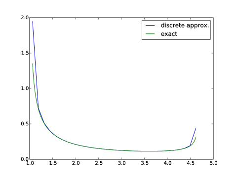
For this example, $p_{j}$ and $\xi$ are independent of $E$. In Figure 1, we compare the Young measure (26) associated with (5) against its discrete approximation (27); in this example, we take $\beta=1$ and, in (27), $m=30$ equispaced values $\sigma_{j}$ between $1$ and $c_{\beta}$, $\beta=1$. Note that the error in the discrete approximation (27) necessarily rises at the end points, since the density $d\lambda_{E}\left(\xi\right)$ is infinite at $\sigma=1$ and $\sigma=c_{\beta}$.

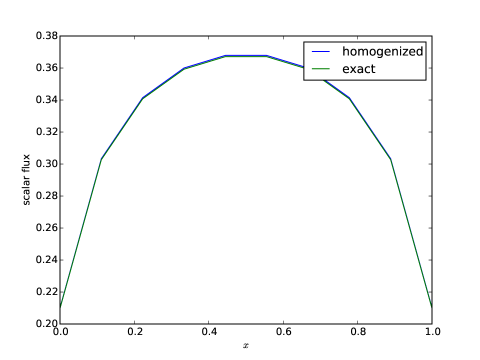
Using (27) in (22)-(23), we then obtain the (approximate) homogenized solution $\psi_{0}\left(x,\mu,E\right)$. In Figure 2, we compare the “exact” scalar flux (24) against its homogenized version (25), where $\psi_{0}$ is computed from (27) and (22)-(23). We use $m=30$ equispaced values $\sigma_{j}$ between $1$ and $c_{\beta}$, $\beta=1$, and a single group $\left[E_{0},E_{1}\right]=\left[0,1\right]$.

Figure 1: Comparison of the Young measure (26) and its discrete approximation (27). We use $m=30$ “band boundaries” $\sigma_{j}$ in (27).

Figure 2: Comparison of the exact scalar flux (24) against its discrete approximation (25), using $m=30$ equispaced values $\sigma_{j}$ between $1$ and $c_{\beta}$, $\beta=1$, and a single group $\left[E_{0},E_{1}\right]=\left[0,1\right]$.

4.2 A neutron transport example with absorption cross section for iron

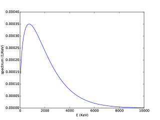
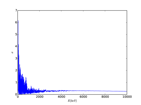
Figure 3: Watt fission spectrum

Figure 4: Absorption cross section for iron.

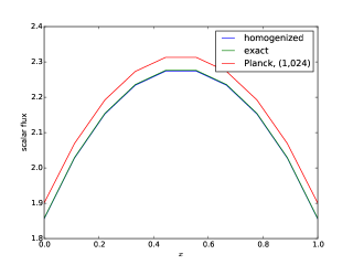
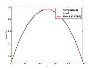
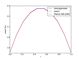
Figure 5: Comparison of the exact scalar flux (24) against its homogenized approximation (25) and the multigroup method with Planck-weighted cross sections, using (a) $1,2024$, (b) $4,096$, (c) $16384$, and (d) $65,536$ equally spaced groups. Here the cross section is for iron as shown in Figure 4.

(a)

(b)

(c)

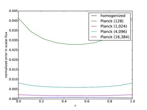
Figure 6: Relative error of the homogenized scalar flux (25), as compared to the exact scalar flux (24), using the cross section for iron shown in Figure 4.

We consider a neutron transport example in slab geometry, which describes the uncollided neutron flux and is useful in shielding applications. In particular, in equation (20), we take $\sigma_{\varepsilon}\left(E\right)$ to correspond to the absorption cross section of iron at room temperature over the energy range $50$ keV to $10$ MeV, as displayed in Figure 4; energy/cross-section pairs $\left(E_{j},\sigma_{j}\right)$ for iron at were generated via the NJoy problem and the cross section $\sigma_{\varepsilon}\left(E\right)$ at a general value $E$ is evaluated via linear interpolation. The subscript $\varepsilon$ on $\sigma_{\varepsilon}\left(E\right)$ is retained for notational consistency, and represents the characteristic resonance spacing; note, however, that $\varepsilon$ is not a free parameter. We use a source term $S\left(E\right)$ corresponding to a Watt fission spectrum,

$$\begin{aligned} S(E)&=c\exp\left(-E/a\right)\sinh\sqrt{bE}\end{aligned},$$

with $a=0.988$ MeV, $b=2.2249$ MeV^-1, and $c=\exp\left(-ab/4\right)/\sqrt{\left(\pi a^{3}b/4\right)}$ MeV^-1 a normalization constant.

As in Section 4.1, we compare the exact scalar flux (24) (that is, exact to within angular discretization errors) against its homogenized version (25). We take $4$ energy groups $\left[E_{i},E_{i+1}\right]$, where the group boundaries $E_{i}$ are equally spaced between $E_{\min}=50.002$ (KeV) and $E_{\max}=10^{4}$ (KeV) Within each energy group $\left[E_{i},E_{i+1}\right]$, we use $m=40$ equispaced values $\sigma_{j}$ between

$$\sigma_{\min,i}=\min_{E_{i}\leq E\leq E_{i+1}}\sigma_{\varepsilon}\left(E\right),$$

and

$$\sigma_{\max,i}=\max_{E_{i}\leq E\leq E_{i+1}}\sigma_{\varepsilon}\left(E\right).$$

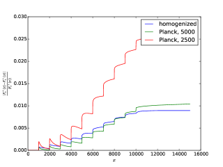
In Figure 5, we compare the homogenized scalar flux with the exact scalar flux, as well as with the scalar flux obtained using the multigroup method with $1,024$, $16,384$, and $65,536$ equally groups. Figure 6 displays the relative errors in the scalar for in the homogenized scalar flux and the scalar flux using the Planck-weighted opacities; we see from this figure that the homogenized scalar flux and the multigroup method $16,384$, achieves about a $.1$ percent relative error in comparison to the exact scalar flux. Recall that the homogenization approach used $4\times 40=160$ energy discretization parameters, and so for this accuracy this translates into orders of magnitude fewer parameters. We note that, for a larger error, the efficiency gain of the homogenized approach in this example is much less significant.

4.3 An atmospheric TRT example with water vapor

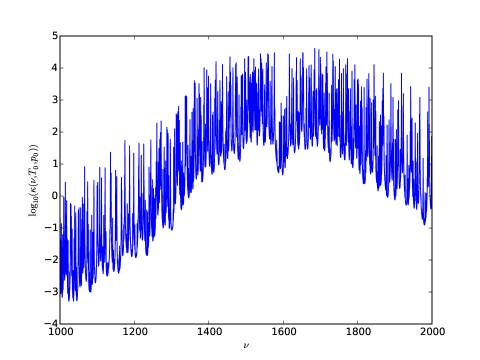
Figure 7: Cross-section $\kappa\left(\nu,T,p\right)$ (kg/m^2) for water vapor as a function of frequency (1/cm), with $T=288.15$ (K) and $p=8.9874\times 10^{4}$ (Pa).

Table 1: Temperature and pressure values in each homogeneous layer.

Height (km)	Temperature (K)	Pressure (Pa)	volume fraction (unitless)
0-1	281.65	8.98746E+4	.0081
1-2	275.15	7.94952E+4	.0077
2-3	268.65	7.01085E+4	.0059
3-4	262.15	6.16402E+4	.0028
4-5	255.65	5.40199E+4	.0016
5-6	249.15	4.71810E+4	.0008
6-7	242.65	4.10607E+4	.0003
7-8	236.15	3.55998E+4	7.96E-5
8-9	229.65	3.07425E+4	3.21E-5
9-10	223.15	2.64363E+4	1.78E-5
10-12	216.65	1.93304E+4	6.94E-6
12-15	216.65	1.20446E+4	3.84E-6

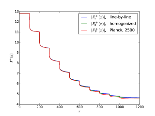
Figure 8: Comparison of the outgoing flux using solutions of the exact and homogenized equations (30) and (32). In solving (30) using the homogenization approach, we use $10$ energy groups and $5$ bands. We also solve (30) using $2500$ and $5000$ Planck-weighted opacities. Plot (a) shows the exact $F_{\varepsilon}^{+}\left(x\right)$ and homogenized outgoing fluxes $F_{0}^{+}\left(x\right)$ (homogenized) and $F_{P}^{+}\left(x\right)$ (Planck). Plot (b) shows the relative errors in the homogenized solution and the Planck solutions.

(a)

(b)

We consider an atmospheric model problem consisting of $12$ homogeneous layers of constant temperature $T\left(x\right)=T_{k}$ and pressure $p\left(x\right)=p_{k}$ for $x_{k}\leq x\leq x_{k+1}$ (see e.g. [10]); for consistency with traditional notation, we consider the frequency variable $\nu$ in place of the energy variable $E$. We solve the TRT equations using cross-sections $\hat{\sigma}\left(\nu,T,p\right)$, corresponding to water vapor, over the frequency range $1000-2000$ (1/cm). As standard for infrared atmospheric TRT calculations, we neglect scattering and assume slab (i.e., plane parallel) geometry. We also use the 1976 U. S. Standard Atmosphere values for temperature and pressure in each layer, as displayed in Table 1. In addition, the volume fraction of water vapor in each layer is also shown in Table 1.

The cross-sections $\hat{\sigma}\left(\nu,T,p\right)$ (in units of kg/m^3) are computed using the HITRAN database and assuming a Lorenz shape profile; in our calculations, we use the Julia module by J. Bloch-Johnson, https://github.com/jsbj/Jultran.jl/blob/master/src/Jultran.jl, for processing the HITRAN files in order to generate the opacities. Here $\log_{10}\left(\hat{\sigma}\left(\nu,T,p\right)\right)$ is plotted in Figure 7 for $T=288.15$ (K) and $p=8.9874\times 10^{4}$ (Pa).

We now describe the problem in more detail. In each homogeneous layer $x\in\left[x_{k},x_{k+1}\right]$, $1\leq k\leq 12$, the intensity $\psi_{\varepsilon}\left(x,\mu,\nu\right)$ satisfies the transport equation

$$\mu\partial_{x}\psi_{\varepsilon}^{k}\left(x,\mu,\nu\right)+\sigma_{\varepsilon}\left(\nu,T_{k},p_{k}\right)\psi_{\varepsilon}^{k}\left(x,\mu,\nu\right) = \sigma_{\varepsilon}\left(\nu,T_{k},p_{k}\right)B\left(\nu,T_{k}\right),$$ (28)

$$\psi_{\varepsilon}^{k}\left(x_{k},\mu,\nu\right) = \psi_{\varepsilon}^{k-1}\left(x_{k},\mu,\nu\right),\,\,\,\,\,\,\,\,\mu>0,$$ (29)

$$\psi_{\varepsilon}^{k}\left(x_{k+1},\mu,\nu\right) = \psi_{\varepsilon}^{k+1}\left(x_{k+1},\mu,\nu\right),\,\,\,\,\,\,\,\,\mu<0.$$ (30)

Here $B\left(\nu,T\right)$ denotes the Planck function; $\sigma_{\varepsilon}\left(\nu,T_{k},p_{k}\right)=r_{k}\rho_{k}\hat{\sigma}_{\varepsilon}\left(\nu,T_{k},p_{k}\right)$, where $\rho_{k}$ and $r_{k}$ denote the density of air (kg/m^3) and the fraction of water vapor in the $k$th layer and $\hat{\sigma}_{\varepsilon}\left(\nu,T_{k},p_{k}\right)$ denotes the cross-section corresponding to water vapor. We also take boundary conditions

$$\psi_{\varepsilon}\left(x_{0},\mu,\nu\right) = B\left(\nu,T_{0}\right),\,\,\,\,\mu>0,$$

$$\psi_{\varepsilon}\left(x_{K+1},\mu,\nu\right) = 0,\,\,\,\,\mu<0.$$

For the homogenized transport equation (10), we use in each spatial interval $\left[x_{k},x_{k+1}\right]$, $k=1,\ldots,12$, seven logarithmically spaced values $\kappa_{ij}\left(T_{k_{0}}\right)$, $j=1,\ldots,7$, for each each frequency group $\nu\in\left[\nu_{i},\nu_{i+1}\right]$ and for the reference temperature $T_{k_{0}}$ for layer $k_{0}=6$ (we find that the error is relatively insensitive to this choice); that is, for each frequency group $\left[\nu_{i},\nu_{i+1}\right]$, the bands $\log\left(\kappa_{ij}\left(T_{k_{0}}\right)\right)$, $j=1,\ldots,5$, are equally spaced between the minimum $\min_{\nu_{i}\leq\nu\leq\nu_{i+1}}\log\left(\sigma_{\varepsilon}\left(\nu,T_{k_{0}},p_{k_{0}}\right)\right)$ and the maximum $\max_{\nu_{i}\leq\nu\leq\nu_{i+1}}\log\left(\sigma_{\varepsilon}\left(\nu,T_{k_{0}},p_{k_{0}}\right)\right)$. For values of $k\neq k_{0}$ (i.e., other spatial intervals), we compute values $\kappa_{ij}\left(T_{k}\right)$ using equation (19) and the techniques discussed in Section 3.4.

From $\kappa_{ij}\left(T_{k}\right)$, we solve

$$\mu\partial_{x}\Psi_{ij}^{k}\left(x,\mu,\nu\right)+\kappa_{ij}\left(T_{k}\right)\Psi_{ij}^{k}\left(x,\mu,\nu\right) = \kappa_{ij}\left(T_{k}\right)B_{i}\left(T_{k}\right),$$ (31)

$$\Psi_{ij}^{k}\left(x_{k},\mu,\nu\right) = \Psi_{ij}^{k}\left(x_{k-1},\mu,\nu\right),\,\,\,\,\,\,\,\,\mu>0,$$ (32)

$$\Psi_{ij}^{k}\left(x_{k},\mu,\nu\right) = \Psi_{ij}^{k}\left(x_{k+1},\mu,\nu\right),\,\,\,\,\,\,\,\,\mu<0,$$ (33)

where

$$B_{i}\left(T_{k}\right)=\int_{\nu_{i}}^{\nu_{i+1}}B\left(\nu,T\right).$$

Given $\Psi_{ij}^{k}\left(x,\mu,\nu\right)$ the homogenized solution $\psi_{0}$ is computed via

$$\psi_{0}\left(x,\mu,\nu\right)=\sum_{j}p_{ij}\Psi_{ij}^{k}\left(x,\mu,\nu\right),\,\,\,\,x\in\left[x_{k},x_{k+1}\right],\,\,\,\nu\in\left[\nu_{i},\nu_{i+1}\right],$$

where $p_{ij}$ denotes the probability that $\sigma_{j}\leq\sigma_{\varepsilon}\left(\nu,T_{k_{0}},p_{k_{0}}\right)\leq\sigma_{j+1}$ for $\nu_{i}\leq\nu\leq\nu_{i+1}$ (recall that $k_{0}=6$ is taken for the reference layer).

In the line-by-line solution of (30), we discretize in angle using $n_{\mu}=8$ Gaussian quadrature nodes $\mu_{p}$ and weights $w_{p}$, and $n_{\nu}=200,001$ equally spaced frequency points in $1000\leq\nu\leq 2000$. In each spatial interval $\left[x_{k},x_{k+1}\right]$, we directly evaluate the analytic solution using $n_{x}=100$ equally spaced spatial points. For example, for $\mu>0$, we proceed from the first spatial interval $\left[x_{1},x_{2}\right]$ to the last spatial interval $\left[x_{11},x_{12}\right]$ and directly evaluate the analytic solution

$$\psi_{\varepsilon}^{k}\left(x,\mu,\nu\right)=e^{-\left(\sigma_{\varepsilon}\left(\nu,T_{k},p_{k}\right)/\mu\right)\left(x-x_{k}\right)}\psi_{\varepsilon}^{k-1}\left(x_{k},\mu,\nu\right)+\left(1-e^{-\left(\sigma_{\varepsilon}\left(\nu,T_{k},p_{k}\right)/\mu\right)\left(x-x_{k}\right)}\right)B\left(\nu,T_{k}\right),$$

at $n_{x}$ equally spaced points $x_{k}\leq x_{q}^{k}\leq x_{k+1}$, with $x_{1}^{k}=x_{k}$ and $x_{n_{x}}^{k}=x_{k+1}$.

Similarly, in the solution of (32), we discretize in angle using $n_{\mu}=8$ Gaussian quadrature nodes $\mu_{p}$ and weights $w_{p}$, and $10$ frequency groups $\left[\nu_{i},\nu_{i+1}\right]$. In each spatial interval $\left[x_{k},x_{k+1}\right]$ and each energy group $\left[\left[\nu_{i},\nu_{i+1}\right]\right]$, we use $7$ bands $\kappa_{ij}\left(T_{k}\right)$, that are equally spaced on a logarithmic scale. As in the solution of (30), we directly evaluate the analytic solution using $n_{x}=100$ equally spaced spatial points. For example, for $\mu>0$, we proceed from the first spatial interval $\left[x_{1},x_{2}\right]$ to the last spatial interval $\left[x_{12},x_{13}\right]$ and directly evaluate the analytic solution

$$\Psi_{ij}^{k}\left(x,\mu\right)=e^{-\left(\kappa_{ij}\left(T_{k}\right)/\mu\right)\left(x-x_{k}\right)}\Psi_{ij}^{k-1}\left(x_{k},\mu\right)+\left(1-e^{-\left(\kappa_{ij}\left(T_{k}\right)/\mu\right)\left(x-x_{k}\right)}\right)B_{i}\left(T_{k}\right),$$

at $n_{x}$ equally spaced points $x_{k}\leq x_{q}^{k}\leq x_{k+1}$, with $x_{1}^{k}=x_{k}$ and $x_{n_{x}}^{k}=x_{k+1}$.

In Figure 8, we compare the line-by-line outgoing flux

$$F_{\varepsilon}\left(x\right)=\sum_{p=1}^{n_{\mu}}\sum_{i=1}^{n_{\nu}}w_{p}\mu_{p}\left(\nu_{i+1}-\nu_{i}\right)\psi_{\varepsilon}\left(x,\mu_{p},\nu_{i}\right),$$

against its homogenized version

$$F_{0}\left(x\right)=\sum_{p=1}^{n_{\mu}}\sum_{i=1}^{n_{G}}w_{p}\mu_{p}\psi_{0}\left(x,\mu_{p},\nu_{i}\right).$$

We also compare the exact outgoing flux that against that obtained using $5000$ Planck-weighted opacities. Plot (a) shows the line-by-line solution, the solution using $2500$ and $5000$ Planck-weighted frequency groups, and the homogenized solution using $10$ frequency groups and $7$ bands . We see from plot (b) in Figure 8 that, for a comparable error, the homogenized solution requires about $70\times$ fewer parameters than the solution obtained via Planck-weighted frequency groups.

References

• [1] Gregoire Allaire. Homogenization and two-scale convergence. SIAM Journal on Mathematical Analysis, 23(6):1482–1518, 1992.
• [2] A.Β Arking and K.Β Grossman. The influence of line shape and band structure on temperatures in planetary atmospheres. Journal of the Atmospheric Sciences, 29(2):937–949, 1972.
• [3] J.M. Ball. A version of the fundamental theorem for young measures. In M.Β Rascle, D.Β Serre, and M.Β Slemrod, editors, PDEs and Continuum Models of Phase Transitions, volume 344 of Lecture Notes in Physics, pages 207–215. Springer Berlin Heidelberg, 1989.
• [4] Etienne Bernard, Francois Golse, and Francesco Salvarani. Homogenization of transport problems and semigroups. Mathematical Methods in the Applied Sciences, 33(10):1228–1234, 2010.
• [5] A.Β S. Besicovitch. Almost Periodic Functions. New York: Dover, 1954.
• [6] D.E. Cullen and G.C. Pomraning. The multiband method in radiative transfer calculations. Journal of Quantitative Spectroscopy and Radiative Transfer, 24(2):97 – 117, 1980.
• [7] Laurent Dumas and Francois Golse. Homogenization of transport equations. SIAM Journal on Applied Mathematics, 60(4):1447–1470, 2000.
• [8] W.Β M. Elsasser. Mean absorption and equivalent absorption coefficient of a band spectrum. Physical Review, 54:126–129, 1938.
• [9] Q.Β Fu and K.Β N. Liou. On the correlated k-distribution method for radiative transfer in nonhomogeneous atmospheres. Journal of the Atmospheric Sciences, 49:2139?2156, 1992.
• [10] Richard Goody, Robert West, Luke Chen, and David Crisp. The correlated-k method for radiation calculations in nonhomogeneous atmospheres. Journal of Quantitative Spectroscopy and Radiative Transfer, 42(6):539 – 550, 1989.
• [11] R.Β E. MacFarlane. The NJOY Nuclear Data Processing System. Los Alamos National Laboratory, LA-UR-12-27079 Rev 2012.
• [12] A.Β Marshak and A.B.Β (Eds.) Davis. 3D Radiative Transfer in Cloudy Atmosphere. Springer, 2005.
• [13] Julien Mathiaud and Francesco Salvarani. A numerical strategy for radiative transfer problems with higly oscillating opacities. Applied Mathematics and Computation, 221:249 – 256, 2013.
• [14] M.Β Modest and H.Β Zhang. The full-spectrum correlated-k distribution for thermal radiation from molecular gas-particulate mixtures. Journal of Heat Transfer, 124:30–38, 2001.
• [15] M.Β F. Modest. Radiative Heat Transfer. Academic Press, 2013.
• [16] G.C. Pomraning. Grey radiative transfer. Journal of Quantitative Spectroscopy and Radiative Transfer, 11(6):597 – 615, 1971.
• [17] S.Β E. Strom and R.Β L. Kurucz. A statistical procedure for computing the line-blanketed model stelar atmospheres with applications to the {F5}{IV} star procyon. Journal of Quantitative Spectroscopy and Radiative Transfer, 6(5):591 – 607, 1966.
• [18] Luc Tartar. Memory effects and homogenization. Archive for Rational Mechanics and Analysis, 111(2):121–133, 1990.