Mufasa: Galaxy Formation Simulations With Meshless Hydrodynamics
Abstract
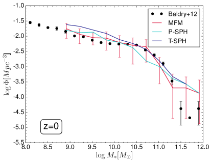
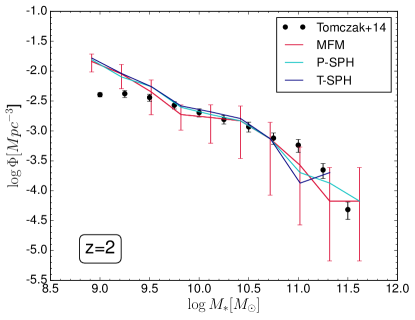
We present the Mufasa suite of cosmological hydrodynamic simulations, which employs the Gizmo meshless finite mass (MFM) code including -based star formation, nine-element chemical evolution, two-phase kinetic outflows following scalings from the Feedback in Realistic Environments zoom simulations, and evolving halo mass-based quenching. Our fiducial volume is evolved to with a quarter billion elements. The predicted galaxy stellar mass functions (GSMF) reproduces observations from to in cosmic variance, providing an unprecedented match to this key diagnostic. The cosmic star formation history and stellar mass growth show general agreement with data, with a strong archaeological downsizing trend such that dwarf galaxies form the majority of their stars after . We run and volumes to with identical feedback prescriptions, the latter resolving all hydrogen-cooling halos, and the three runs display fair resolution convergence. The specific star formation rates broadly agree with data at , but are underpredicted at by a factor of three, re-emphasizing a longstanding puzzle in galaxy evolution models. We compare runs using MFM and two flavours of Smoothed Particle Hydrodynamics, and show that the GSMF is sensitive to hydrodynamics methodology at the level, which is sub-dominant to choices for parameterising feedback.
keywords:
galaxies: formation, galaxies: evolution, methods: N-body simulations, galaxies: mass function1 Introduction
Galaxies were first identified over a century ago, yet the physical processes that shape their observable characteristics and evolution remain poorly understood. With the growth of large-scale structure now well specified within the concordance Lambda Cold Dark Matter (CDM) paradigm, the least understood issues surround how the baryonic components behave once the dark matter’s gravity is no longer the dominant driver. In particular, much of the uncertainty lies in the nature and physics of feedback processes, i.e. the energy return from processes of star and black hole formation within galaxies that self-regulates their growth. As observations of the galaxy population from the present day back to the epoch of reionisation continue to improve, it is an increasingly demanding challenge for models to reproduce such observations using well-motivated and comprehensive input physics, while giving insights into the physical processes responsible for feedback and galaxy assembly.
Successful modern galaxy formation models generally rely on the following basic ingredients (Somerville & Davé, 2015): (i) Fueling of star formation via gravitationally-driven gas accretion from the intergalactic medium (IGM); (ii) feedback from massive, young stars that drives large-scale galactic outflows; and (iii) feedback from supermassive black hole accretion that suppresses star formation in massive galaxies. The goal of galaxy formation models is thus to understand and constrain the physics driving these various feedback processes, and particularly how they work in concert to shape galaxies as we observe them via multi-wavelength surveys across cosmic time.
Cosmological hydrodynamic simulations have played a major role in the progress towards understanding galaxy formation. The past decade has seen significant advances in both the size and dynamic range of simulations thanks to advancing computing power, as well as the scope and accuracy of the input physics thanks to an improved understanding of the key physical drivers. Such simulations are now able to broadly reproduce primary demographic features of the galaxy population today, along with their evolution to early epochs, to reasonable levels of success (e.g. Davé, Oppenheimer, & Finlator, 2011; Davé, Finlator, & Oppenheimer, 2011; Vogelsberger et al., 2014; Genel et al., 2014; Schaye et al., 2015; Somerville & Davé, 2015). However, all cosmological-volume models still require “sub-resolution” recipes for feedback processes, because despite heroic computational efforts it remains infeasible to simultaneously resolve the physics driving feedback at sub-parsec scales within a megaparsec-scale structure formation context. While current models are typically tuned to reproduce key observations such as a galaxy stellar mass function to within a factor of several, they accomplish this using widely differing input physics and numerical implementations, making it difficult to draw robust conclusions regarding the detailed physical processes driving feedback.
One way forward in order to hone in on viable sub-resolution recipes for feedback is to utilise the results of very high-resolution simulations of individual galaxies that examine specific feedback processes in detail. This has recently been greatly enabled by the “zoom” simulation technique in which a particular galaxy and its surroundings are extracted from a larger volume and re-simulated at much higher resolution. In this way, feedback processes are generated more self-consistently and tracked more directly (e.g. Hopkins et al., 2014; Christensen et al., 2016). It is not straightforward to predict population statistics from individual zoom simulations, but their predictions can serve as inputs for the recipes used in cosmological-scale simulations that model many thousands of galaxies.
A particularly comprehensive set of physical processes was included in the Feedback In Realistic Environments (FIRE) zoom simulations (Hopkins et al., 2014). Using the FIRE simulations, Muratov et al. (2015) derived scaling relations for the mass loss rate and velocity distribution of outflowing gas, which are key aspects of star formation-driven feedback. Detailed models for self-shielding (e.g. Faucher-Giguere, Kereš, & Ma, 2010; Rahmati et al., 2013), black hole growth (e.g. Sijacki et al., 2007; Anglés-Alcázar et al., 2015, 2016), and quenching (Gabor et al., 2011) have been investigated to study their emergent trends with a similar strategy in mind. These trends can then be implemented into large-scale, lower-resolution simulations to provide more physically motivated recipes for feedback. Such a multi-scale approach offers a promising avenue to assemble robust and well-constrained recipes for feedback processes within cosmological-scale galaxy formation models.
Another important area of progress has been towards increasing the robustness of hydrodynamics solvers. Early simulations were predominantly done using the Smoothed Particle Hydrodynamics (SPH) technique (Hernquist & Katz, 1989; Monaghan, 1992). However, this method requires substantial artificial viscosity that compromises the handling of surface instabilities, contact discontinuities, and strong shocks. A reformulation of the SPH equations to explicitly conserve entropy provides some advantages (Springel & Hernquist, 2002; Springel, 2005), but still resulted in numerical surface tension that e.g. strongly supresses Kelvin-Hemholtz instabilities (Agertz et al., 2007). Further reformulations such as SPH-S (Read & Hayfield, 2012) and Pressure-SPH (Hopkins, 2013) have partially but not fully mitigated these issues.
Adaptive mesh refinement (AMR) galaxy formation codes have also made substantial gains (e.g. The Enzo Collaboration, 2014), but their intrinsically Cartesian nature can result in numerical artifacts when applied to the arbitrary 3-D geometry and motions associated with galaxy formation. The Voronoi tesselation-based moving mesh code Arepo (Springel, 2010) eliminates the Cartesian restrictions, and shows great promise at handling surface instabilities and shocks with arbitrary geometries while retaining Galilean invariance. A downside is that Arepo advects mass across cell boundaries and occasionally must “re-mesh” to prevent highly deformed cells. This necessitates the additional complication of tracer particles in order to track the motion of gas into and out of galaxies (Genel et al., 2014).
Recently, Hopkins (2015) developed a new “meshless” hydrodynamics method that marries many advantages of SPH and moving mesh approaches. Gizmo is fundamentally a moving mesh-like Godunov code, but the “mesh” is defined by a deformable kernel moving in such a way as to keep the mass within each cell constant. Hence operationally it allows for the advantages of mass tracking and being fully adaptive without re-meshing. Hopkins (2015) showed that Gizmo’s “meshless finite mass” (MFM) approach shows desirable behavior compared to modern SPH and AMR codes in many relevant idealised test problems111http://www.tapir.caltech.edu/~phopkins/Site/GIZMO.html.
In this paper we present a new suite of cosmological hydrodynamic simulations of galaxy formation using Gizmo, called the Mufasa simulations. We describe our new recipes for sub-resolution processes (§2) based on, wherever possible, the results from zoom simulations or analytic models. These include -based star formation, minimal ISM pressurization, non-equilibrium cooling and ionisation, supernova-heated two-phase kinetic winds, evolving halo mass-based quenching, and nine-metal chemical enrichment from Type Ia+II supernovae and stellar evolution. Our highest resolution Mufasa run resolves essentially all hydrogen cooling halos, while our fiducial volume produces a substantial population of quenched massive galaxies by . All are run with exactly the same feedback parameters, and show reasonable resolution convergence. As a basic test of our model, we present predictions for the galaxy stellar mass function across cosmic time, and compare to recent observations and simulations (§3). We further compare to observations of the star formation histories, both globally and for individual galaxies (§4). We also examine the how the choice of hydrodynamics solver and key feedback parameters impact our results (§5). Finally, we summarize our findings (§6).
2 Code Description
2.1 Gizmo gravity and hydrodynamics
We employ a modified version of the gravity plus hydrodynamics solver Gizmo (Hopkins, 2015), which is built upon the framework of the Gadget-3 galaxy formation code (Springel, 2005). For hydrodynamics, we employ Gizmo’s meshless finite mass (MFM) method, which uses a Riemann solver to evolve the fluid in a manner that conserves mass within each fluid element. Each fluid element may then be regarded as a “particle”, though it actually represent a mesh node; we will refer to these as “gas elements.” Like Arepo, Gizmo offers advantages over SPH in terms of handling a wide range of fluid problems related to shocks and contact discontinuities, and over AMR codes in terms of avoiding Cartesian artifacts and strictly preserving Galilean invariance.
We employ a cubic spline kernel with 64 neighbors in MFM. Hopkins & Raives (2015) used 32 neighbors for their detailed MHD simulations, but we discovered that 64 is better for suppressing occasional instabilities in very diffuse hot gas such as that appearing in the shocked IGM at late epochs. The kernel is used to determine the volume partition between gas elements, thereby defining the effective faces at which the Riemann problem is solved.
In order to test the sensitivity to hydrodynamics methodology, we will also use the modern Pressure-SPH (P-SPH; Hopkins, 2013) and the Traditional (entropy-conserving) SPH (T-SPH; Springel & Hernquist, 2002) solvers in Gizmo, with all subgrid physics options held fixed. SPH requires an artificial viscosity, for which we use the Gizmo default Cullen & Dehnen (2010) viscosity as described in Hopkins (2015). To isolate the impact of the hydro solver, we use the same cubic spline kernel with 64 neighbors, even though a quintic spline gives better results in some circumstances 222Dehnen & Aly (2012) found that SPH similar to T-SPH using a cubic spline kernel with 64 neighbors may, in strong shearing flows, be subject to particle pairing instabilities that result in lowering the effective resolution. We thus ran the same T-SPH simulation with a quintic spline with 64 neighbors, and the results were essentially identical. Hence this pairing instability is evidently not impacting our results..
The gravity is evolved using a Tree-Particle-Mesh approach that is based on Gadget-3 (Springel, 2005). We use adaptive gravitational softening throughout for all particles (Hopkins, 2015), enclosing 64 particles with a minimum (Plummer-equivalent) softening length set to 0.5% of the mean interparticle spacing. For more details on Gizmo, including other choices such as the timestep limiter (Durier & Dalla Vecchia, 2012) and the implementation of adaptive softening, see Hopkins (2015).
2.2 Radiative Cooling and Heating
We use the Grackle-2.1 chemistry and cooling library (The Enzo Collaboration, 2014; Kim et al., 2014), which includes primordial and metal line cooling, evolved isochorically on the cooling timescale in an operator-split way over the system timestep. In other words, we do the non-radiative cooling/heating first over the system timestep, then apply radiative cooling using Grackle, where the radiative part is sub-stepped isochorically on the cooling timescale.
We employ Grackle in non-equilibrium mode for primordial elements, thereby tracking e.g. the input of latent heat during reionisation. Metal-line cooling is computed using Cloudy (Ferland, 2004) tables self-consistently including the impact of photoionisation, in this case assuming ionisation equilibrium. A spatially-uniform photo-ionising background is assumed, for which we employ the determination by Faucher-Giguere, Kereš, & Ma (2009), updated in 2011. We do not employ the more recent Haardt & Madau (2012) determination owing to concerns regarding its low H i ionisation rate at which has spurred the so-called photon underproduction crisis (Kollmeier et al., 2014). In any case, galaxy properties that we consider here are insensitive to reasonable choices of the photo-ionising background.
2.3 Star Formation
To form star particles out of gas, we employ a molecular gas-based star formation prescription following Krumholz, McKee, & Tumlinson (2009, hereafter KMT). A fuller description is available in Krumholz & Gnedin (2011) and Thompson et al. (2014); here we briefly summarise the approach.
KMT provides an approximate solver for formation at the (relatively) coarse resolution available to us in cosmological volumes. With well-motivated approximations, this yields
| (1) |
where
| (2) |
where is the metallicity in solar units, is a function of metallicity given in KMT, and is the column density calculated using the Sobolev approximation; see below. We impose a minimum metallicity of solely for the purposes of this computation. We further require a minimum density for star formation of cm-3; gas above this density will hereafter be referred to as “ISM gas”. In most cases, the densities at which dominates is higher than this (e.g. cm-3 for solar metallicity) but for individual high metallicity gas elements the KMT formula can yield formation, and hence star formation, below our ISM density threshold; we explicitly do not allow this.
We make two minor adjustments to the KMT algorithm regarding sub-grid clumping. First, KMT assumed a constant sub-resolution clumping factor in the ISM of . This factor appears in the rate coefficient for forming on dust grains (see §2.2 of Krumholz & Gnedin, 2011). It is clear that a higher resolution simulation should assume less clumping – in the limiting case of infinite resolution, the clumping should be fully resolved and hence should be unity. Thus it makes physical sense to reduce in higher resolution simulations. In our case, we assume that in our fiducial simulation with (see §2.10), where is our minimum comoving gravitational softening length, but we further scale in our other runs (see Table 1). By this scaling, a simulation with pc would have ; our cosmological runs here do not reach this limit. The net effect of scaling is to make star formation slightly less efficient in higher resolution simulations, leaving them slightly more gas rich.
Our second adjustment involves the calculation of . KMT assumes that self-shielding against dissociating radiation within the ISM is governed by the local column density as calculated using the Sobolev approximation, namely where is the gas density. We compute these quantities in the usual way from the gas elements, but we must further account for sub-resolution clumping. If the clumping factor represents the typical density contrast of the sub-resolution clumps, then the column density increase within these clumps is approximately, by dimensional arguments, . We thus increase by a factor of to account for this333 The factor of 10 is appropriate for our fiducial large volume. This factor should vary as varies, but owing to an oversight this was not implemented for the higher-resolution runs. We subsequently ran test simulations to determine that the results are not significantly different if we scale , though it does lower star formation very slightly. Future runs will use this scaling..
Given an fraction from KMT, the star formation rate for a given eligible gas element is given by a (1959) Law, namely
| (3) |
where is the molecular fraction for a given gas element, and is the local dynamical time. We set the efficiency of star formation to be (Kennicutt, 1998).
Star particles are spawned from gas elements stochastically. Each MFM fluid element spawns a single star particle of the same mass. Previous simulations (e.g. Oppenheimer & Davé, 2008) often spawn multiple star particles, reducing the gas mass by a fraction each time. However, large instantaneous changes to an element’s gas mass can cause instabilities in MFM, so we avoid this by converting the gas element fully into a collisionless star particle all at once, conserving mass and momentum.
2.4 Resolving the Jeans mass in the ISM
As the density increases and the cooling rate becomes large, the Jeans mass can become smaller than the resolved mass in the simulation. If cooling is allowed to proceed at these high densities, the fragmentation that should proceed to small scales (and thus be captured by our star formation law) is instead “bottlenecked” at large scales, producing artificially coherent clumping (Schaye & Dalla Vecchia, 2008).
To avoid this, we apply an artificial pressure above a density threshold that explicitly suppresses fragmentation below the scale of the smoothing volume, namely:
| (4) |
where is the molecular weight calculated assuming fully neutral gas, is the mass per gas element in our simulation, and is the number of neighbors.
We assume that the temperature at the density threshold is K. Above this density, we then set the gas element temperature to the Jeans minimum temperature:
| (5) |
If is below our nominal star formation density threshold, we set it to this value; this occurs in our largest volume. Meanwhile, our smallest volume has cm-3, while our intermediate volume has cm-3.
This prescription is quite similar to the equation of state imposed by Schaye & Dalla Vecchia (2008), except that we vary the threshold density with the simulation resolution such that at higher resolution, we do not artifically pressurise the ISM as strongly. Hence our approach automatically takes advantage of high numerical resolution, when present, as much as possible (e.g. Thompson et al., 2016).
2.5 Feedback From Massive Stars
As necessitated by our cosmological resolution, we employ a sub-resolution approach to modeling feedback from massive stars. The basic approach is to use kinetic feedback (Springel & Hernquist, 2003; Oppenheimer & Davé, 2006), as this has generally been shown to provide stable and well-converged results for cosmological galaxy formation simulations, and allows more explicit control over the numerical experiments regarding feedback.
In our feedback prescription, we assume that massive stars launch winds that drive material out of galaxies through a combination of Type II supernovae (SNII), radiation pressure, and stellar winds. We do not track these phenomena in the code owing to a lack of resolution, but rather characterise the net effect using two free parameters, namely the mass loading factor defined as the mass outflow rate relative to the star formation rate, and the wind speed representing the velocity with which the wind is launched. Both parameters can in principle scale with galaxy properties and redshift. Outflow fluid elements are launched in the direction of va, in order to have a broadly collimated outflow perpendicular to the disk, and the sign is chosen such that it is launched in the hemisphere pointing away from the host galaxy. Later we will show that this choice has no discernible impact versus ejecting gas isotropically.
2.5.1 FIRE wind scalings
Our general strategy is to directly employ outflow scalings derived from the FIRE simulations (Hopkins et al., 2014), which self-consistently drive winds from galaxies using supernova feedback, radiation from massive stars, and stellar winds, and have been successful at reproducing a range of observed galaxy properties in individual galaxy zoom simulations.
Muratov et al. (2015) found in the FIRE simulations that the outflow rate was most tightly correlated with stellar mass, and this scaling was essentially independent of redshift. Their best-fit relation of the mass outflow rate at is given by
| (6) |
where is the galaxy stellar mass. We implement this relation directly into our code. We compute using an on-the-fly galaxy finder, which we describe in §2.6. To account for the very early evolution of galaxies when little or no stellar mass has yet formed, we place a floor on the stellar mass used in the above equation of 8 gas element masses.
For the wind speed, we likewise take the scaling of with galaxy properties from the FIRE simulations. Their best-fit formula is , where is the galaxy’s circular velocity. We will describe how we obtain from our on-the-fly galaxy finder in §2.6. In FIRE, this formula reflects the mean velocities across a shell at . To account for the fact that our wind launches are typically at a much smaller radius well within the ISM, we add an extra velocity kick corresponding to the gravitational potential difference between the wind launch radius and (Łokas et al., 2001). We assume a Navarro, Frenk, & White (1997) profile with a concentration , where we compute the halo mass as the galaxy baryonic mass times . This typically increases the wind velocity by up to in small galaxies, and by significantly less in large galaxies.
Still, only accounts for gravitational slowing, while hydrodynamic slowing is likely to be dominant (Oppenheimer & Davé, 2008). Hence we further increase the multiplier of the outflow velocity, by around a factor of two above the Muratov et al. (2015) value, comparable to their 95th percentile wind velocity, and also comparable to the outflow velocities measured leaving the disk in the zoom simulations of Christensen et al. (2016). We choose to normalize this multiplier to the FIRE scaling at . Hence the velocity formula used in Mufasa is
| (7) |
Finally, we add a random tophat scatter of to . The resulting wind launch velocities are typically , which is comparable to the observed maximum outflow speeds in low-redshift (Martin, 2005) and high-redshift (Steidel et al., 2010) galaxies.
2.5.2 Two-phase winds
Winds are often observed to be flowing out of nearby galaxies (e.g. M82) partly in hot gas, putatively heated by supernova explosions and the resulting shocks. Previous kinetic wind models (Davé, Oppenheimer, & Finlator, 2011; Vogelsberger et al., 2014) have generally not included this form of energy injection, even though their simulations lack the resolution to properly capture SNe shock heating in the ISM. Winds are also seen in cool form, mainly via low-ionisation absorption lines. Hence it is clear that there are at least two phases for outflowing gas.
In Mufasa, we model two-phase winds by randomly selecting outflowing gas to be “cool” or “hot”. Cool gas is ejected at K, although they quickly heat to K via photo-ionisation once they are outside the ISM. For the hot wind, we directly employ a fraction of the supernova energy not used for kinetic ejection into thermal heating of the wind. For a Chabrier initial mass function (IMF), each solar mass of stars produces 0.01028 stars with masses above . We assume each of these becomes a supernova which produces ergs, hence the specific energy production from SNe is erg g-1.
The kinetic energy used by the wind is , where we assume that the total wind mass ejected owing to a gas mass of forming into stars is . If each wind fluid element has mass , then the specific energy utilised by the wind is .
The specific thermal energy added to each hot wind gas element is then
| (8) |
If we add no heat; physically, this can represent a situation where other wind mechanisms such as radiation pressure are primarily responsible for driving winds. We have found that so long as the heating raises the typical temperature above a few times K to get it past the Helium and O vi cooling peaks (which almost always does), then the impact on galaxies is relatively insensitive to the exact amount of heating.
We define a free parameter that determines the fraction of the wind that is ejected hot. Each wind element is then randomly chosen to be either hot or cool, based on the probability . In Mufasa, we choose , motivated by ISM-scale simulations of supernova-driven winds that suggest roughly 30% of the material is ejected in hot form (T. Naab, priv. comm.). Hence our two-phase wind is assumed to be majority cool, but containing a substantial component of hot gas.
2.5.3 Hydrodynamic decoupling and recoupling
No hydrodynamics code is able to properly evolve a single fluid element (cell or particle) moving with a high Mach number through its surroundings. This is simply a limitation of resolution, and is not mitigated by the use of an improved hydrodynamics solver in MFM: A single fluid element will never be able to capture the sub-element mixing and dissipation with its surrounding gas. For this reason, it is necessary to make some approximation regarding the interactions of the outflowing gas when passing through the ISM. Ideally, one would like to follow the detailed evolution of gas mixing with its surroundings via surface instabilities, but this is non-trivial, since the Kelvin-Hemholtz mixing time is generally very short. Instead, we follow early works by Springel & Hernquist (2003) and Oppenheimer & Davé (2006, 2008), along with recent simulations such as Illustris (Vogelsberger et al., 2014), and employ decoupled winds. That is, we turn off hydrodynamic forces on outflowing gas until such time as it “recouples” back to its surrounding gas. The physical motivation is that winds are often seen to blow channels through the ISM that likely allow the relatively unfettered escape of a coherent flow. Moreover, this makes physical sense since our outflow scalings are taken from FIRE simulations who measured their wind properties well outside the ISM.
The criteria for recoupling has historically been chosen via a density threshold, e.g. 10% of the ISM density threshold, and a time limit, e.g. enough to free-stream for tens of kpc (e.g. Springel & Hernquist, 2003). Here, we add a new recoupling criterion: That the velocity of the outflowing gas element be similar to its surroundings. This criterion additionally allows recoupling when the gas has a velocity that can be properly handled by the hydrodynamics solver.
Specifically, our recoupling criterion requires that the wind gas element has a velocity difference with respect to surrounding gas of less than 50% of the local sound speed (). The sound speed is calculated from the kernel-weighted temperature of surrounding gas at the wind element’s position, and the velocity difference is summed over all neighbors with kernel weighting. We exclude all other decoupled wind gas when computing quantities for the surrounding gas. Using 20% or 100% rather than 50% did not yield appreciably different results. We further turn off radiative cooling while the wind is decoupled, in order to allow hot gas in the wind to deposit their thermal energy into the circum-galactic medium (CGM).
Gas elements satisfying the mach number criterion are recoupled regardless of surrounding density or time, so long as they have a density that is less than the ISM density. But there are cases where this recoupling criterion is not satisfied for a long while or until far away, particularly in low-mass halos where the outflows are typically ejected into very low density gas. Hence we also employ a density limit of 1% of the ISM threshold density, and a time limit of 2% of the Hubble time at launch which is comparable to a disk dynamical time; reaching either of these criteria automatically triggers recoupling as well. In the end, the total fraction of decoupled gas is always well below 1%, reaching a maximum of around % at .
2.6 Fast, Approximate Friends-of-Friends
Equation 6 requires to determine , and equation 7 requires to determine the outflow velocity. To determine and , we employ a fast approximate friends-of-friend (FOF) galaxy finder on the fly during the simulation run. This FOF finder groups stars and ISM gas into baryonic galaxies. It is approximate because it finds neighbours within a cube of side , where is the linking length, rather than a sphere of radius . This greatly improves computation speed while having minimal impact on the identified galaxies, thus enabling the code to run this FOF finder at essentially every timestep. We calibrate times the mean interparticle spacing in order to obtain the same mass function as that obtained by using the Spline Kernel Interpolative Denmax (SKID; e.g. Kereš et al., 2005) galaxy finder. Our results are insensitive to variations in by a factor of a few around our chosen value, but we choose this value since it is the minimum hydrodynamic kernel size, which is 40% of the minimum softening length, multiplied by 2.8 which is the conversion from Plummer equivalent softening to the actual smoothing kernel radius. Hence we link particles that are within one (minimum) kernel length of each other.
This FOF finder yields groupings of star particles and gas elements, from which we compute the baryonic mass and . Given , we then determine for use in our outflow scalings by employing the observed baryonic Tully-Fisher relation (McGaugh et al., 2012) with a redshift evolution as expected from Mo, Mao, & White (1998), namely
| (9) |
where is Hubble’s constant at redshift .
2.7 Feedback From Long-Lived Stars
Type Ia supernovae (SNIa) and asymptotic giant branch (AGB) stars provide additional energetic feedback. These components provide feedback that is substantially delayed relative to the time of star formation, hence are not represented by our kinetic outflows and must be included separately. Typically, delayed feedback is energetically sub-dominant relative to the processes that drive winds, but they may be important in particular circumstances, hence we include their contributions for completeness.
The SNIa rate is modeled following Scannapieco & Bildsten (2005) as a prompt component that is concurrent with SNII, and a delayed component that emerges from stars and begins after an age of 0.7 Gyr. The rates are taken from Sullivan et al. (2006), namely SNIa yr for the prompt component, and SNIa for the delayed component (see Oppenheimer & Davé, 2008, for further details).
Each SNIa is assumed to add erg of energy to the surrounding gas. The prompt component energy is added at each timestep to each star-forming gas element, and the delayed component is added to the 16 nearest gas elements to the given star, in a kernel-weighted fashion. To save computation time, we do the delayed feedback for stars only at specific intervals, with the interval scaling roughly inversely with the age of the star, from a minimum of every timestep for ages under 200 Myr to a maximum of every 10 timesteps for stars 2 Gyr and older.
AGB star feedback also adds energy to surrounding gas. We implement the model of Conroy, van Dokkum & Kravtsov (2015) in which AGB stellar winds are assumed to thermalise with the ambient gas. First, we compute the stellar mass loss rate assuming a Chabrier (2003) initial mass function using a lookup table based on Bruzual & Charlot (2003) models. We then calculate the energy deposition rate based on the mass loss rate and the velocity difference of the star relative to each neighboring gas element. We again use the 16 nearest neighbors, in a kernel-weighted fashion. We add the velocity of the stellar wind to this, which we assume to be 100 km/s (Conroy, van Dokkum & Kravtsov, 2015). In practice, even this large wind stellar velocity that is on the upper end of plausibility makes a negligible difference for most galaxies. This is because if the energy is added to star-forming gas it will quickly radiate away. However, such energy could potentially accumulate into making a substantial impact if the stars are embedded primarily in hot gas, such as in a cluster environment; we will examine this in more detail in future work.
2.8 Chemical Enrichment
Delayed feedback mechanisms also deposit heavy elements into the surrounding gas. We track the evolution of 11 elements, including hydrogen, helium, and 9 metals: C, N, O, Ne, Mg, Si, S, Ca, and Fe. These elements comprise over 90% of metal mass in the universe.
For SNII yields, we use Nomoto et al. (2006), parameterised as a function of metallicity; we interpolate the yields to the metallicity of the given gas element being enriched. We are using essentially the same yield tables used in Oppenheimer & Davé (2008), which in Davé, Finlator, & Oppenheimer (2011, and other studies) was found to result in metallicities that are too high by a factor of compared to the observed mass-metallicity relation. In previous studies (e.g. Davé et al., 2013; Liang et al., 2016) we have simply rescaled metallicities in post-processing, arguing that such changes do not greatly impact the dynamics, and that the predicted yields are uncertain at this level. However, given that cooling and -based star formation rates depend on metallicity, it is more accurate to reduce the yields during the simulation run. For this reason, we multiply all Type II SN yields by a factor of 0.5. We add all SNII energy to the star-forming gas element itself, in the instantaneous self-enrichment approximation. On cosmological timescales, and with sufficient star-forming gas within a given galaxy, this yields a well-converged metallicity distribution.
For SNIa yields, we employ Iwamoto et al. (1999), assuming each SNIa yields of metals. The prompt SNIa component, like TypeII enrichment, is done in the instantaneous self-enrichment approximation, while the delayed feedback components are added to the 16 nearest gas element surrounding the given star in a kernel-weighted manner.
For AGB stars, we follow Oppenheimer & Davé (2008) and employ a lookup table as a function of age and metallicity in order to obtain the yields; these yields come from several sources, as described in Oppenheimer & Davé (2008). We additionally assume 36% helium fraction and a nitrogen yield of 0.00118. The enrichment, like the energy, is added from stars to the nearest 16 gas elements, kernel-weighted, following the mass loss rate as computed assuming a Chabrier (2003) IMF.
For the KMT model, we need to provide a total metallicity in solar units, for which we assume a solar abundance taken from Asplund et al. (2009). We do not include metal diffusion or mixing in these models to avoid an extra free parameters, since it is unclear how much metal mixing should be occuring (Schaye, Carswell, & Kim, 2007).
| Name | |||||||||||
|---|---|---|---|---|---|---|---|---|---|---|---|
| m50n512 | 50 | 0.5 | 0.20 | 0.98 | 1.11 | 0.23 | 1.32 | 1.97 | |||
| m25n512 | 25 | 0.25 | — | —- | 1.04 | 0.08 | 1.24 | 1.00 | |||
| m12.5n512 | 12.5 | 0.125 | — | —- | 0.19 | 0.02 | 0.38 | 0.26 |
is the box size in comoving .
is the minimum gravitational softening length in comoving (equivalent Plummer).
is the galaxy stellar mass resolution limit in (32 star particle masses).
2.9 Quenching Feedback
With only stellar feedback as described above, massive galaxies still form stars too rapidly and the stellar mass function is not truncated at the high mass end (e.g. Gabor & Davé, 2010). Hence an additional “maintenance mode” source of energetic feedback is required to fully quench massive galaxies (e.g. , 2006; Somerville et al., 2008). Here we follow the model in Gabor & Davé (2012, 2015), who argued that keeping gas hot in massive halos is sufficient to yield quenched massive galaxies in agreement with mass function and red sequence observations.
We quench galaxies by heating all gas in massive halos except gas that is self-shielded. We compute the self-shielded cold gas fraction for each gas element using the prescription described in Rahmati et al. (2013), which parameterises the effective strength of the photo-ionising background impinging on gas as a function of density and redshift. This ionising background strength is then used to compute the cold gas fraction (which includes both neutral and molecular gas) using a rate balance equation as described in Popping et al. (2009). Gas is considered self-shielded if its cold gas fraction after applying self-shielding is above 10%. By only heating non-self-shielded gas, most of the neutral and molecular hydrogen within hot halos is unaffected, ensuring that these cold gaseous components are only directly affected by physical processes such as stripping rather than our quenching prescription.
We apply this quenching heating in massive halos with a mass that exceeds the quenching mass given by
| (10) |
This formula is obtained from the analytic equilibrium model of Mitra, Davé, & Finlator (2015) as the best-fit parameterization of required to match various observational constraints from .
Gas in halos above that is not self-shielded and is below the virial temperature is heated to 20% above virial temperature at each timestep. We calculate K (Voit, 2005), where we obtain the halo mass using a friends-of-friends algorithm with a linking length of 0.16 times the mean interparticle spacing. This FOF algorithm is different than the one used to compute and , and is only run every 0.5% of a Hubble time only on dark matter particles since it has substantial computational cost; gas and star particles are linked to halos via their nearest dark matter particle.
We stress that this is a phenomenological model intended to capture the most important effects of whatever microphysics actually drive quenching. Specifically, we are not saying that halos simply “self-quench” in the simulations (owing to e.g. virial shocks or simple cooling physics). Quite the opposite: if we only include hydrodynamics, cooling, star formation, and stellar feedback physics, we see far too much star formation at high masses, as noted above. This model directly requires some additional feedback mechanism to be the source of (considerable) additional energy to maintain the virial temperatures of halo gas. The physical mechanisms of this feedback remain uncertain, however – hence the empirical model adopted here. The most likely candidate is feedback from a super-massive black hole, which many groups have shown can plausibly inject sufficient energy far out in the halo and resolve the cooling flow problem (, 2006; Somerville et al., 2008; Schaye et al., 2015). In future work, we will explore what the empirical model here requires in terms of energetic input, and how this compares to e.g. the kinetic luminosity function of AGN jets. In these simulations (with kpc resolution), however, any model for black hole formation/seeding, dynamical evolution, merging, fueling/growth, and feedback would be necessarily sub-resolution. As such, we would in any case simply adjust the sub-resolution parameters until they produced the same effects as our quenching model here. Our method here thus allows us to more directly isolate what needs to occur on resolved scales in the simulation, in order to match massive galaxy observations.
2.10 Runs
All simulations assume a cosmology consistent with Planck (2015) “full likelihood” constraints: , , , , , and . We generate initial conditions with these parameters using Music (Hahn & Abel, 2011). Each runs begins at in the linear regime.
Our fiducial simulation consists of a randomly-selected cubical cosmological volume, with additional simulations used to examine early galaxy evolution having and box sizes (these are separate runs, not sub-volumes extracted from the larger run). Each run evolves gas fluid elements (i.e. mass-conserving cells) and dark matter particles. With these choices, the volume’s halo mass resolution (i.e. 64 dark matter plus 64 gas elements) is , which means that this run resolves essentially all hydrogen cooling halos back to the earliest epochs. We will also show results from , element runs to examine variations in hydrodynamics methodology.
Table 1 lists our main Mufasa run parameters. The 50 boxes is evolved to a final redshift of , while the 25 and volumes down to owing to both computation expense and the fact that these volumes are too small to be representative at later epochs. We also list the galaxy stellar mass resolution limit in each run, taken to be 32 star particle (or equivalently, gas element) masses. We have found that stellar mass functions are generally well-converged to this limit, but other quantities such as star formation histories can require a higher mass threshold for convergence (e.g. Davé, Oppenheimer, & Finlator, 2011).
We output 135 snapshots down to (85 to ) for each run. We analyse the snapshots using SPHGR444http://sphgr.readthedocs.org/en/latest/ (Thompson, 2015), which identifies galaxies using SKID and halos using RockStar (Behroozi et al., 2013), and then links them via their positions. SPHGR goes on to calculate many basic properties of the galaxies and halos such as and SFR, and finally outputs a Python “pickle” file for each snapshot that contains all this information, including member particle lists. All plots in this paper are produced directly from these SPHGR pickle files.
3 Stellar Mass Functions
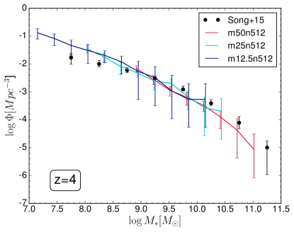
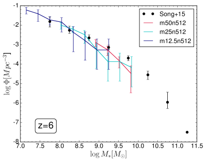
The primary observational benchmark for testing galaxy formation models is the galaxy stellar mass function (GSMF). The GSMF has now been measured robustly out to , covering about 90% of cosmic stellar mass buildup, thanks in particular to improving deep near-infrared surveys such as the Cosmic Assembly Near-IR Deep Extragalactic Legacy Survey (CANDELS; Grogin et al., 2011; Koekemoer et al., 2011) and the FourStar Galaxy Evolution Survey (ZFOURGE; Tomczak et al., 2014). Measurements at higher redshifts are also improving rapidly (e.g. Duncan et al., 2014; Song et al., 2015), though they typically rely on less certain conversions between ultraviolet luminosity and stellar mass. Matching the GSMF and its evolution is thus a key test of whether a model reproduces the bulk of galaxy growth over cosmic time.
It remains a significant challenge for galaxy formation models, be they semi-analytic (SAMs) or hydrodynamic, to match the GSMF to within uncertainties at all redshifts (Somerville & Davé, 2015). SAMs can reproduce the GSMF quite well, typically because they are tuned to do so, while hydrodynamic simulations have recently achieved improved levels of success with discrepancies at . Moving to higher redshifts, most models overproduce the GSMF below the knee at , and some underproduce the GSMF at . These differences show up prominently when considering the star formation histories of galaxies, where models characteristically deviate from that inferred for real galaxies particularly at lower masses in the sense of having overly early stellar growth in low-mass galaxies (White et al., 2015). In this section, we will test the Mufasa simulations against observations using the evolution of the GSMF from .
3.1 Comparisons to observations
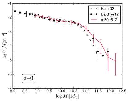
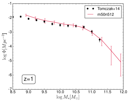
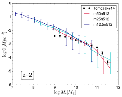
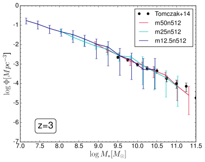
Figure 1 shows the GSMF from our Mufasa simulations at . The three box sizes are colour-coded as navy blue (), cyan (), and crimson red (). Only galaxies with stellar masses above the galaxy mass resolution limit listed in Table 1 are included in each case. We compare to observations (black circles, with Poisson errors) at from the Galaxy and Mass Assembly (GAMA) Survey by Baldry et al. (2012) and from Bell et al. (2003), at to combined CANDELS and ZFOURGE data from Tomczak et al. (2014), and at to CANDELS data from Song et al. (2015). For Tomczak et al. (2014), to obtain the GSMF at we average the quoted values at and weighted by the number of galaxies in each bin, and analogously we compute a weighted average of and to obtain the points shown; for , we quote the results, which is likely a slight overestimate. While we only choose to compare to one data set so we can more easily engage in quantitative statistical comparisons, various current GSMF observations do not differ significantly at (e.g. Somerville & Davé, 2015).
In Table 1, we quote a reduced value comparing the simulation data to observational data at each redshift, for each run. To obtain this, we compute error bars on the simulation values as the variance in the GSMF over eight sub-octants of each simulation volume. This approximately accounts for both cosmic variance and Poisson errors, though generally the Poisson errors are sub-dominant. This then produces error bars (asymmetric in log space), which are displayed in Figure 1. We then compute from these error bars in log (not linear) space, so that a GSMF that is e.g. low by a factor of 2 will have the same as one that is high by a factor of 2. We sum over the range of overlapping masses between the simulation and the data, using the upper error bar if the data is higher than the simulation, otherwise the lower error bar. To get a reduced we divide by the number of observed data points. These values provide a quantitative assessment of the level of agreement between Mufasa runs and the observed GSMF.
We note that this value of does not take into account uncertainties in the observations themselves, but as can be seen in Figure 1 from the statistical error bars shown on the observed points, these uncertainties are generally sub-dominant to cosmic variance uncertainties. There are additional systematic errors in observed GSMF determinations which can be quite significant particularly at high redshifts, but we also ignore these since these are difficult to quantify accurately (see e.g. Mobasher et al., 2015, for more discussion). We also note that we are comparing SKID-derived masses in simulations to (typically) aperture-based masses from various observational samples, which may introduce a significant bias particularly at high masses () where high-Sercic profiles create extended wings in the surface brightness distribution (Genel et al., 2014; Kravtsov, Vikhlinin, & Meshscheryakov, 2014). Hence the comparisons at the highest masses should be regarded with some additional observational uncertainty, but our values for are generally driven by low- where our cosmic variance errors are smaller. Finally, we note that our cosmic variance errors may still be underestimated owing to our smaller volume, as Genel et al. (2014) found somewhat larger uncertainties from 25 sub-volumes in Illustris. All of these additional aspects would go towards lowering our quoted values.
We now examine how well the mass functions agree with observations at various redshifts. At , our fiducial Mufasa run is in remarkably good agreement with the Baldry et al. (2012) GSMF. It faithfully reproduces the observed low-mass slope down to our galaxy mass resolution limit, showing that our star formation feedback algorithm does very well at properly suppressing the low-mass end. At high masses, there is a sharp turnover towards an exponential that has been difficult to achieve in previous models, and highlights the success of translating the evolving quenching mass determined from the equilibium model of Mitra, Davé, & Finlator (2015) into full hydrodynamic simulations. There may be a very slight overproduction of the highest mass galaxies, albeit well within cosmic variance uncertainties, but we note that there is some uncertainty in the masses of massive ellipticals owing to how the galaxy is separated from intracluster light (Kravtsov, Vikhlinin, & Meshscheryakov, 2014). As listed in Table 1, the reduced at this redshift relative to Baldry et al. (2012), which quantifies the excellent agreement with observations. The agreement is slightly less good veresus Bell et al. (2003), with , driven mostly by the reduced high-mass GSMF in this determination.
At , the Mufasa mass function is in good agreement with the Tomczak et al. (2014) observations, with . There is a slight excess in the sub- range; this becomes more prominent at , which has a comparable . The disagreement is driven most strongly by the lowest observed point, which may also be the most uncertain owing to incompleteness in the observations. In contrast, Reddy & Steidel (2009) determined a steeper faint-end slope of from rest-UV observations, in much better agreement with Mufasa. Upcoming observations with the James Webb Space Telescope should definitively settle this issue.
At we see, in both the observations and the simulation, a turn-down at the highest masses where our quenching model starts to suppress massive galaxy growth. At this redshift, , which means that galaxies with can begin to be affected. The onset of quenched massive galaxies between is in general agreement with observations (e.g. Kriek et al., 2009). Interestingly, the most actively star-forming galaxies in the universe at have halo masses of (Wilkinson et al., 2016), which corroborates our value of at these epochs.
Since our smaller volumes are evolved to , we can here examine the resolution convergence among all three volumes. Broadly, the three runs lie within cosmic variance uncertainties of each other. However, in detail we see that there is a systematic trend that higher resolution simulations produce slightly higher mass functions in the overlapping mass range. Over a factor of 64 in mass resolution between the and volumes, the mass function at is increased by about a factor of two. At higher masses, the GSMF in the smallest volume start to drop low because it cannot form enough massive galaxies. The interpolates this trend, being slightly higher at low- compared to the fiducial volume, and slightly lower at high-. We note that the values for the smaller volumes are still close to unity, so the agreement with data is still satisfactory, although in part this owes to our smaller volumes having larger cosmic variance uncertainties.
At , all the volumes’ GSMFs are essentially power laws over the modeled mass range. The agreement is excellent with all three simulations, with . However, we note that the data used is actually from galaxies at , so at it is possible that the data should be slightly lower than indicated. Hence as a check we analyzed a simulation output and compared with this data, and still found very good agreement with . The resolution convergence among the three volumes here, as well as at all higher redshifts, is excellent.
At higher redshifts (), we begin to see slight discrepancies at the high-mass end, in the sense that the Mufasa runs do not produce enough high-mass galaxies. It is already slightly evident at – while the smallest volume has , the larger volumes show . The discrepancy becomes somewhat more significant at , particularly in the volume, where . The other volumes, probing only lower masses, are not as strongly discrepant, having at . This discrepancy could be the result of the very high bias of early massive galaxies, which reside in large halos that are not properly represented even in the volume. Alternatively, it could be that the limited resolution does not capture very early star formation in the largest density perturbations. Hence both resolution and volume effects go towards underproducing early stellar mass. We note that another high- GSMF determination from CANDELS by Duncan et al. (2014) yields generally higher values, which would be further discrepant; the determination from Grazian et al. (2015), on the other hand, are comparable to that of Song et al. (2015). Nonetheless, it is worth noting that are at present substantial systematic uncertainties in deriving stellar masses at these redshifts.
We note that at , and particularly at , the observational GSMF determinations are subject to significant systematic uncertainties, and various determinations often lie significantly outside each others’ formal statistical uncertainties (Ilbert et al., 2013; Muzzin et al., 2013; Tomczak et al., 2014; Mobasher et al., 2015). For this reason, one should use caution in interpreting the agreement or lack therefore with models at these redshifts, as improving observations may shift these values non-trivially. Nonetheless, much of the disagreement between data sets occurs at high-, whereas our is driven by our agreement at low- where our cosmic variance errors are small. For now, we claim that our agreement is comparably good against most recent data sets at these redshifts, but that future observational determinations may yet alter this.
In summary, Mufasa does an excellent job of matching the observed GSMF from , in all cases to within in simulation cosmic variance. This agreement is unprecedented, and suggest that Mufasa achieves an impressive level of realism in modeling galaxy stellar growth across cosmic time. The agreement at the massive end owes to our evolving halo quenching mass, and suggests that this simple description provides a good match to the truncation of star formation across cosmic time (as argued e.g. in Gabor & Davé, 2012, 2015). It also illustrates the synergy between constraints derived from the analytic equilibrium model and detailed hydrodynamic simulations. At high redshifts, the data are still subject to significant systematic uncertainties, hence we await upcoming deeper observations particularly using the James Webb Space Telescope to more robustly constrain these models. Nonetheless, our high-resolution simulations agree quite well with currently available reionisation-epoch GSMF observations, suggesting that simulations that resolve all H-cooling halos are robust for such studies. Our runs also show reasonable resolution convergence, albeit with a noticeable trend for higher-resolution simulations to produce slightly higher GSMFs at the low-mass end.
3.2 Comparison to other simulations
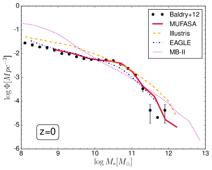
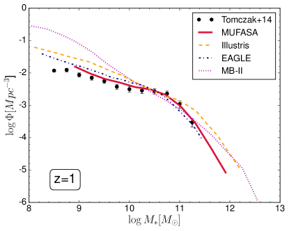
Recently, major cosmological galaxy formation simulation projects have set new standards for the number of fluid elements and input physics. Illustris (Vogelsberger et al., 2014; Genel et al., 2014), EAGLE (Schaye et al., 2015; Crain et al., 2015), and MassiveBlack-II (MB-II; Khandai et al., 2015) each model around fluid elements, making them the (computationally) largest cosmological hydrodynamic simulations of galaxy formation evolved to to date. Illustris employs Arepo, EAGLE uses a modern SPH variant, and MB-II uses Gadget-3 with entropy-conserving SPH (Springel, 2005). While the dynamic range of these simulations is a remarkable computational achievement, it is still insufficient to directly model the feedback processes that regulate galaxy evolution. Hence like Mufasa, they utilize subgrid representations for star formation and black hole feedback in order to suppress galaxy growth. The differences in their GSMF predictions are likely driven primarily by variations in feedback recipes, as opposed to variations in hydrodynamic methodology (see e.g. Hopkins, 2013, and §5.1).
Illustris and MassiveBlack-II employ decoupled winds, phenomenologically similar to Mufasa. Illustris uses scalings for energy-driven winds, namely ; this is similar to that predicted from high-resolution zooms by Christensen et al. (2016), although the amplitude assumed in Illustris is many times higher. MB-II uses a constant mass loading factor and wind speed similar to the original Springel & Hernquist (2003) recipe. Such a “constant wind” model gives roughly the correct global stellar mass density, but does not fare as well at reproducing GSMFs (e.g. Oppenheimer et al., 2010; Davé, Oppenheimer, & Finlator, 2011). EAGLE, in contrast, does not decouple winds, but rather assumes that ISM gas particles accumulate SN energy until they can be instantaneously heated to a high temperature, typically K where cooling times are long and hence the thermal pressure can drive an outflow. While hydrodynamics remain turned on, cooling is effectively turned off as the particle accumulates SN energy, which occurs for tens of dynamical times, and hence this model is also phenomenological. In this way, the approach has similarities to the blast wave cooling shutoff model of e.g. Governato et al. (2007) and Stinson et al. (2013). Nonetheless by tuning this presciption, it is possible to nicely reproduce the stellar mass function, with a key aspect being that the given amount of supernova energy from star formation is preferentially injected into higher density gas (Crain et al., 2015). While differing in approach, all these simulations have claimed to be in broad agreement with observations of the GSMF.
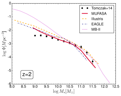
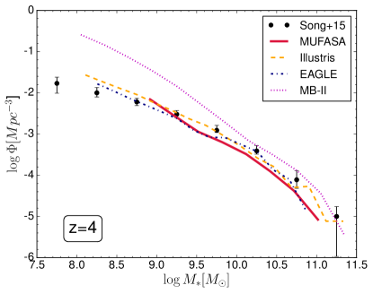
In Figure 2 we compare the GSMF of the Mufasa fiducial run to the Illustris simulation (Vogelsberger et al., 2014, orange dashed line;), the EAGLE reference model (McAlpine et al., 2015, dark blue dashed line;), and the MassiveBlack-II simulation (magenta dashed line; Khandai et al., 2015) at and 4. The first two are reproduced from Somerville & Davé (2015), while the latter data was kindly provided by A. Tenneti and T. DiMatteo. We omit error bars that were shown in Figure 1 to better see the differences, but we include the same observations as were shown in that figure for reference.
At , the Mufasa and EAGLE simulations both do an excellent job of reproducing the observed GSMF, with Mufasa doing somewhat better at capturing the sharp knee of the mass function. Crain et al. (2015) describes the process of tuning EAGLE’s input physics in order to obtain this agreement, though it is worth noting that their mass function mostly emerged rather naturally, and much of the tuning was done to match galaxy sizes. In our case, we mostly constrained our input physics using higher-resolution simulations or analytic models, but we still had to mildly tune some parameters such as the outflow velocity. Meanwhile, Illustris clearly overproduces galaxies at both low and high masses, and only agrees well around (i.e. the knee). MassiveBlack-II shows the characteristic steep mass function that their “constant wind” feedback model is known to produce, which greatly overpredicts small galaxies and underpredicts the GSMF around (see also Davé, Oppenheimer, & Finlator, 2011).
At , the discrepancies between simulations and data starts to grow, particularly below . All the simulations overpredict the low-mass end to varying levels. Illustris and MB-II are quite high, and EAGLE is mildly high compared to observations. Mufasa also overpredicts the low-mass end, but to a lesser extent than any other model, making it clearly the best fit to the intermediate-redshift GSMF.
At , the discrepancies seen at for low mass galaxies persist; generally, the simulations are signficantly higher than observations here, with Mufasa providing the closest match. At the massive end, Illustris and MB-II nicely reproduce the turnover, but EAGLE cuts off the GSMF at too low a mass. Mufasa also truncates the GSMF slightly early, albeit less so than EAGLE. Part of this may owe to the smaller box size of Mufasa, relative to the other simulations which have box sizes.
At , Illustris and EAGLE do somewhat better than Mufasa, as our fiducial Mufasa run produces too low a GSMF. Our volume which has comparable resolution to those runs, as well as our run, show better agreement as seen in Figure 1. As mentioned previously, the deficit in the run may owe to the lack of resolution to start galaxy growth early enough, combined with the lack of volume required to include growth of the largest halos. Nonetheless, Mufasa is still within of cosmic variance, so it is possible that the chosen initial conditions unluckily do not produce enough early massive galaxies.
While the Mufasa runs presented here lack a dynamic range comparable to these larger simulations, they do offer several modeling advantages. Compared to MassiveBlack-II, Mufasa employs a hydro solver that has been shown to yield better results for key test problems (Hopkins, 2015), and additionally our outflow scalings better reproduce the observed GSMFs at the low-mass end. Compared to Illustris, Mufasa reproduces observed GSMFs significantly more closely over most of cosmic time. Generally, EAGLE and Mufasa yield comparably good mass functions, with Mufasa slightly better from Cosmic Noon until today, and EAGLE slightly better at . Mufasa has some disadvantages as well. Besides less dynamic range, we also do not yet explicitly track central black hole growth and feedback as the other simulations do (this is in progress; see e.g. Anglés-Alcázar et al. 2016). Nevertheless, compared to recent state-of-the-art galaxy formation simulations, Mufasa generally is as good or better at reproducing the observed stellar mass buildup in galaxies across the majority of cosmic time as traced by the GSMF.
4 Galaxy Growth Rates
4.1 Global star formation rate density
The growth of galaxy stellar mass is reflected in the star formation rates of galaxies across cosmic time. A key barometer of this is the evolution of the cosmic star formation rate density (SFRD), commonly known as a Lilly-Madau plot. We note that the cosmic SFRD is not an ideal test of models, because it is an integrated quantity that can be sensitive to observational integration limits, and individual simulations only cover a limited range of the total cosmic star formation. Hence discrepancies compared to observations may reflect limitations of volume or resolution rather than intrinsic model failings. Nonetheless, the SFRD evolution is a oft-used benchmark and highlights some important points about the characteristics of galaxy growth.
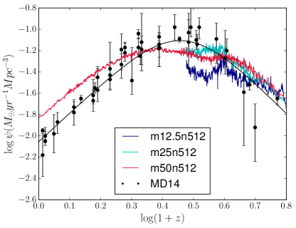
Figure 3 shows the cosmic star formation rate density () evolution as a function of . Our three volumes () are shown as the crimson, cyan, and navy blue lines respectively. Here, we have plotted the SFR directly output during the simulation run as the stellar mass formed per unit time, which displays small-timescale fluctuations owing to the stochastic nature of our star formation algorithm; this employs no selection criterion, and even includes star formation in unresolved galaxies. For comparison, data from a recent compilation by Madau & Dickinson (2014) is shown in black, including a line for their global best-fit relation along with the individual compiled data points; these have been divided by 1.7 in order to correct from their assumed Salpeter IMF to a Chabrier IMF.
The fiducial simulation qualitatively follows the observed trend faithfully: There is a rapid rise of from , then it is relatively constant until , and then it falls rapidly towards the present day. The evolution since generally follows the power-law expectation from cosmological accretion, as has been noted by many previous works (e.g. Somerville & Davé, 2015). In detail, Mufasa underpredicts the global SFR during Cosmic Noon (which we will discuss in §4.4), and overpredicts the SFR at lower redshifts () by about 50%. This is particularly curious in light of the good agreement with the evolution of the GSMF. It is also opposite to the discrepancy versus the recent models such as Illustris, EAGLE, and the SAM of Henriques et al. (2015), which tend to underpredict the SFRD at low- while still generally agreeing with GSMF evolution. The SFRD peak at is also broader in Mufasa than in the data, which likewise mimics the trend in other current models. It is not obvious how one reconciles all these models and observations; in part it may reflect systematic uncertainties in star formation rate measures, or suggest that a more careful comparison should be done to account for observational selection effects. We will break this down versus in §4.4 to gain more insights into the differences.
The run matches the quite well over the redshift range probed. This is a bit of a coincidence, as we have seen in the GSMF that the low-mass end is slight overproduced in this run, which appears to compensate for the lack of high-mass star-forming galaxies owing to the smaller volume. For the run, this coincidental balance fails, as the lack of high-mass star forming galaxies dominates over the mild excess production at low masses. As a result, begins to lie significantly below that of the larger volumes at . There is also significant stochasticity over long timescales at (in addition to the short stochasticity) because the global star formation is dominated by a handful of the most massive galaxies whose star formation rates can vary substantially. Overall, the small-volume results are seen to be not cosmologically representative at in terms of large galaxy growth, but the evolution of dwarf galaxies should still be robust. At , all our volumes’ SFRD values agree with each other, and are within the uncertainties of the Madau & Dickinson (2014) data.
In summary, the SFRD evolution from is broadly reproduced in our Mufasa runs. This is not surprising given the fact that the GSMF matches reasonably well at all redshifts . The deviations at in the volume highlight incompleteness at the massive end owing to its small volume; deviations at lower redshifts will be discussed §4.4.
4.2 Star formation downsizing
A key characteristic of the galaxy population is known as “downsizing”, first coined by Cowie et al. (1996), in which star formation shifts from more massive galaxies to lower-mass galaxies over time. This results in more massive galaxies having older stellar populations, which has been dubbed “archaeological downsizing” (Thomas et al., 2005). While downsizing has been referred to as anti-hierarchical, the qualitative trend is a natural outcome of hierarchical structure formation, since the largest galaxies arise in the largest density perturbations which are able to collapse and start forming stars first (Neistein, Dekel, & van den Bosch, 2006). Nonetheless, quantitatively reproducing the observed growth rates of galaxies as a function of mass has proved challenging for models.
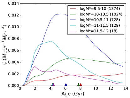
Since the fiducial Mufasa simulation well reproduces the observed stellar mass function covering over 90% of cosmic star formation, it provides a quantitative picture of downsizing as a function of galaxy mass. Figure 4 illustrates this. Here, we show the star formation history of galaxies subdivided into five bins of stellar mass, from to . The time at which half the present-day stellar mass was formed is indicated by the colour-coded upward arrows along the bottom of the plot, for each mass bin. Note that this is computed by examining the formation times of the remaining stellar mass at , which is different than the star formation rate in those galaxies at any particular epoch, owing to the effects of stellar mass loss; in general, the median star formation rate will be shifted to slightly earlier times. This also makes no distinction between stellar mass that was formed in the main progenitor versus accreted satellite galaxies. In this sense, our depiction here is most closely related to archaeological downsizing.
Downsizing is clearly evident here – higher mass galaxies have earlier formation epochs. Galaxies with , which are predominantly quenched today, have median stellar formation times around Gyr, or close to . Galaxies with in contrast have formation times of Gyr, i.e. . Galaxies around the knee of the mass function today dominate the global stellar mass, and have a median formation time of around 6 Gyr, or . Hence our simulations naturally predict that more massive galaxies will host older stellar populations.
The smallest galaxies have a global star formation rate that steadily increases with time all the way to the present day, which is qualitatively different than galaxies that end up around the knee of the GSMF. Such star formation histories in dwarfs are qualitatively what is required to solve the so-called dwarf galaxy conundrum, in which current models generically predict dwarf galaxy star formation histories that peak at too early epochs (White et al., 2015). We will examine this so-called dwarf galaxy conundrum using Mufasa in more detail in future work.
4.3 Stellar mass density evolution
A complementary view of galaxy growth is provided by the evolution of the cosmic stellar mass density. In principle, this should be equivalent to an integral of the Lilly-Madau plot, accounting for stellar evolution. Some discrepancies between these two approaches have been claimed in the past (e.g. Wilkins, Trentham, & Hopkins, 2008; Davé, 2008), but these have been contradicted by more recent data (Reddy et al., 2012; Madau & Dickinson, 2014); the issue remains unsettled.
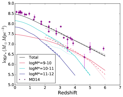
Figure 5 shows the evolution of the cosmic stellar mass density in our three simulations; solid, dashed, and dotted lines correspond to our , and runs respectively. We also show the breakdown in three ranges of stellar mass, the dwarf (), (), and massive () galaxy regimes, colour-coded as indicated in the legend. Finally, the cyan points show some recent (post-2010) data from the compilation of observations by Madau & Dickinson (2014), namely Moustakas et al. (2014) at low redshifts, Ilbert et al. (2013), Muzzin et al. (2013), and Reddy et al. (2012) out to , and Gonzalez et al. (2011), Lee et al. (2012), and Caputi et al. (2011) to higher redshifts.
The total stellar mass density evolution is generally in good agreement with observations. At the box falls slightly below the data, potentially owing to observed galaxies extending to masses below the resolution limit of this simulation. The discrepancy is never more than 30%, nonetheless it is interesting that this contrasts with the predictions for the Lilly-Madau plot, which show an overprediction of the observed SFRD at these redshifts. This hints at some mismatch between the observed global growth of stars versus the observed global star formation rates. At high redshifts the agreement is very good, although the data shows more scatter there.
Breaking down by mass, at early epochs the total mass density is dominated by relatively small galaxies, since larger galaxies have not yet formed. By , galaxies above begin to dominate the mass density, which continues all the way until the present day. Larger galaxies do not dominate at early times since few have formed, and do not dominate at late times since their growth is suppressed by quenching. Examining the various box sizes by comparing lines of the same colour, we see that there is generally good convergence even when broken down by mass, though there are variations of up to about 50%.
Overall, Mufasa simulations do a good job of reproducing the cosmic stellar mass density evolution, and the variations between the different resolution boxes is not large. Together with the good match to the Lilly-Madau plot, this demonstrates that Mufasa provides a viable suite of models with which to examine global stellar mass growth.
4.4 Specific star formation rates
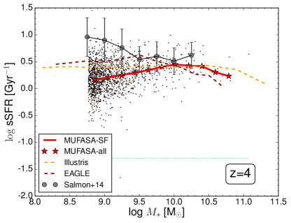
A key test of how galaxies grow is the evolution of the star formation rate–stellar mass relation, often called the star-forming galaxy “main sequence” (Noeske et al., 2007). Now measured out to and beyond, its evolution has proved to be challenging for models to reproduce particularly during Cosmic Noon (), with both SAMs and simulations typically predicting specific star formation rates (sSFRs) at that are too low by (Daddi et al., 2007; Davé, 2008; Sparre et al., 2015; Somerville & Davé, 2015). Many of these same models, however, also tend to overpredict the GSMF during Cosmic Noon by roughly the same factor, so it has been conjectured that a model that matches the GSMF at (and keeps the SFRs the same) would also match the main sequence. Since the Mufasa simulations provide a reasonable fit to the GSMF at , it is interesting to examine whether they likewise matches the main sequence at these epochs.
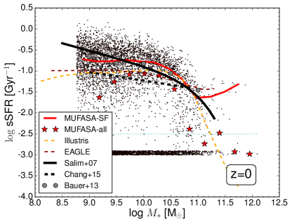
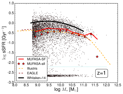
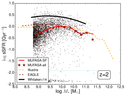
Figure 6 shows sSFR vs. at in our fiducial Mufasa simulation. Along the bottom are depicted galaxies with very low (typically zero) sSFR, with some artificial spread to enhance visibility. The red solid line shows the running median sSFR as a function of , for star-forming galaxies defined as those above the cyan dashed line lying just above the quenched galaxies. The stars indicate a binned median for all galaxies, including the quenched ones. Observations are shown in black: At , we show a Schechter-form fit from Salim et al. (2007, solid black) based data from the Sloan Digital Sky Survey (SDSS) and the Galaxy Evolution Explorer (GALEX), as well as H-based star formation rate determinations from the Galaxy Mass and Assembly (GAMA) survey by Bauer et al. (2013, gray points). We also show a fit to the recent SDSS+Wide Infrared Survey Explorer (WISE) determination by Chang et al. (2015, dashed black). At we show data from 3D-HST with Spitzer 24m information by Whitaker et al. (2014), and at from CANDELS by Salmon et al. (2015). Finally, for comparison we show results from the Illustris (orange dashed) and EAGLE (dark red dashed) simulations.
At , Mufasa star-forming galaxies show a flat low-mass end and a turn-down at as the general population starts to be quenched (but is still regarded as star-forming by our cut). The predictions are in very good agreement with recent H-based SFR’s from GAMA (Bauer et al., 2013, grey circles), and in reasonable agreement with the SDSS+GALEX data from Salim et al. (2007), However, they are higher than the sSFR’s inferred from full m SED fitting including WISE data (Chang et al., 2015). It is beyond the scope of this paper to assess the various differences in observations, but we note that even the present-day SFRs are somewhat controversial.
For comparison, we show results from Illustris (orange; ) and EAGLE (dark red; ) simulations, which like Mufasa show a flat sSFR() at low masses (see also Davé, Oppenheimer, & Finlator, 2011), but with an amplitude that is lower by . These are generally in better agreement with the Chang et al. (2015) data. Hence even simulations that nicely match the GSMF such as Mufasa and EAGLE can have substantially different sSFR values for star-forming galaxies. As mentioned earlier, the global SFRD in these other simulations tend to be lower than that in Mufasa, and from the sSFR comparison this is likewise seen to be the case for individual galaxies with . There are also a handful of massive Mufasa galaxies that are still star-forming as well, which contribute non-trivially to the global SFRD. We will examine the massive galaxy population and its colours in an upcoming paper.
The stars show the binned median values from Mufasa now including the quenched galaxies. Such galaxies dominate by number at low and high masses – the median values (stars) at and are actually in the quenched population. At low masses these are typically stripped satellites, while at high masses they are quenched centrals. Observations generally do not suggest quite such a dominant population of low-mass quenched satellites, but such satellites are also difficult to observe, so selection effects may be important. We leave a more thorough investigation of central vs. satellite populations for future work.
Moving to , the Mufasa predictions clearly lie below the data, typically by a factor of up to 2 relative to the Whitaker et al. (2014) data across the resolved mass range. Illustris and EAGLE are comparable. Indeed, such a discrepancy is generically seen among models of all types (Somerville & Davé, 2015). The number of quenched galaxies is markedly less, so that the medians are now generally within the star-forming population.
At , the agreement gets even worse – the deficit of Mufasa versus the Whitaker et al. (2014) data is now across most of the mass range. This is comparable to or even lower than the predictions from Illustris (Sparre et al., 2015) and EAGLE (Schaye et al., 2015). There are very few quenched galaxies by this epoch, so one cannot easily appeal to burstiness to explain the discrepancy – besides the fact that the observed tight main sequence scatter limits the contribution of starbursts (Rodighiero et al., 2011).
This discrepancy at remains a major puzzle, and it starkly contrast with the fact that Mufasa nicely reproduces the evolution of the GSMF around this redshift range. If the Universe is producing stars at a rate times higher than Mufasa at , and the GSMF agrees at , then where do all those stars end up? They don’t appear to produce an excess in the observed GSMF relative to Mufasa at ; if anything, Mufasa lies slightly above the observed GSMF at . Hence it seems that the rate of stellar growth as tracked by the GSMF is not straightforward to reconcile with that measured directly via star formation rates. It could be that the observed star formation rates are simply too high owing to calibration issues, but the uncertainties in UV+24m star formation rates are generally thought to be significantly smaller than the discrepancy. As the conjecture in Bastian, Covey, & Meyer (2010) states, any problem in galaxy formation can be resolved with a suitable choice of IMF, and in this case a top-heavy or bottom-light IMF remains a viable if unpopular solution (Wilkins, Trentham, & Hopkins, 2008; Davé, 2008).
The discrepancy could also be solved by raising values at by via some unforeseen systematic errors. Given that current GSMF data at this epoch is now based on deep near-IR data that probes well beyond the 4000Å break, it would be quite surprising if the stellar mass estimates were so far off; current methods for estimating typically do not differ systematically by such large amounts (Mobasher et al., 2015). Furthermore, this would shift the GSMF to quite high values, and would result in their being more massive galaxies at than today. Hence this solution seems untenable.
Finally, at the dynamic range spanned by observations is relatively small, but the disagreements versus the data are clearly less, particularly for larger star-forming galaxies. Mufasa shows little trend with mass at this redshift, and perhaps even has a positive slope at . The Salmon et al. (2015) data plotted shows a rise towards the lowest masses that at face value is divergent from the model predictions, but incompleteness in identifying low-SFR galaxies via Lyman break selection at these redshifts may mitigate this disagreement. The discrepancy in sSFR() versus models thus seems to be primarily restricted to Cosmic Noon (), as has long been noted (e.g. Davé, 2008).
In summary, Mufasa shows similar trends to previous models in matching observations at low and high redshifts, but falling low throughout Cosmic Noon. At there are substantial differences versus recent simulations at the low-mass end, with Mufasa showing higher levels of present-day star formation in star-forming dwarfs, although quenched dwarfs dominate by number. At intermediate redshifts, Mufasa mimics the shape if not amplitude of sSFR(), with a positive sSFR() slope at low masses and a negative one at high masses. The high observed sSFR values across all masses at remain a persistent quandary for modern galaxy formation models, even ones that match the observed GSMF evolution through that epoch.
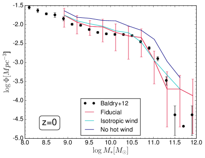
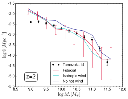
5 Code variations
A major advantage of Gizmo is that it has the ability to trivially switch between four hydrodynamic solvers while holding all other input physics fixed. Hence it provides an ideal platform for testing the sensitivity of results such as the GSMF to hydrodynamic methodology. To contextualise the differences resulting from numerical methodology, we explore how key input physics choices change the GSMF.
5.1 Sensitivity to hydrodynamics methodology
Gizmo contains four hydrodynamics solvers: MFM, which is our fiducial choice; meshless finite volume (MFV), which is a mass-advecting moving mesh-like scheme; pressure-SPH (P-SPH; Hopkins, 2013), which is a pressure-energy formulation of SPH that improves surface instability handling; and traditional SPH (T-SPH), which is a density-energy formulation of SPH. These are described in more detail in Hopkins (2015, Appendix F). We note that T-SPH employs some new features in Gizmo relative to older SPH codes, such as an improved artificial viscosity and artificial conduction; see Hopkins (2015) for details. Since MFV does not strictly conserve mass within fluid elements (though it does so approximately), it is not obvious how reliably it will function with the kinetic outflows, stellar mass loss, etc., hence we will not consider this scheme here. Instead, we will focus on comparing the mass-conserving schemes MFM, P-SPH, and T-SPH.
Figure 7 shows the GSMF at (left) and (right) in runs with MFM, P-SPH, and T-SPH. These runs have a box size of and particles, but in every other way are identical to our fiducial Mufasa run, excepting the hydro solver which is only identical for the MFM case. Observations are shown as described in Figure 1 for reference, although the focus here is on comparing among the hydro solvers rather than comparing to data. Error bars are again computed as cosmic variance over eight sub-octants within each simulation volume (only shown for the MFM case; the others are similar but omitted for clarity), and they are larger than in the full Mufasa run owing to the smaller volume.
We first note that the MFM run produces a GSMF that is statistically identical to the run. This is not surprising, as they have identical numerical resolution and input physics, but it is reassuring that these simulations display good GSMF convergence with volume, even though there are many fewer galaxies in the smaller volume.
Comparing amongst the various hydro solvers, at early epochs () the GSMFs are very similar. In other words, kinetic outflows are suppressing early galaxy formation in a manner that is essentially independent of the hydro solver. Indeed, the differences at (not shown) are even smaller.
By , the three hydro solvers diverge non-trivially in their predictions. As discussed in Oppenheimer et al. (2010), the contribution from wind recycling (i.e. the re-accretion of previously ejected material) to stellar mass growth starts to be significant at , and becomes dominant by . Our preliminarily interpretation is thus that the differences between hydro solvers owe primarily to differences in the way that galactic outflows interact with the surrounding medium and rejoin the accretion flow. This is consistent with the idea that the main improvement in MFM over SPH is handling two-phase instabilities and shocks, which are important mechanisms for how winds interact with circum-galactic gas.
T-SPH tends to produce about more galaxies at any given compared to P-SPH. Meanwhile, both SPH codes produce a steeper GSMF than MFM. In Oppenheimer et al. (2010), it was noted that the flattening of the GSMF in the sub- regime is achieved in simulations by wind recycling. If this is likewise the case in these simulations (as we expect), then we can infer that winds recycle more effectively in MFM than in SPH.
The detailed reasons for these variations are not entirely obvious. Our preliminary interpretation for difference between P-SPH and T-SPH is as follows. In flows with large variations of internal energy from particle-to-particle, P-SPH, because it kernel-averages the pressure over all neighbors’ as opposed to just using the particle’s times density, a single very high- particle can raise the pressure of all its neighbors. This means that all of them together can do more PdV work than a single hot particle could. While this is done in an energy-conserving way, it can effectively enhance the ability of lone, hot particles to add substantial pressure. In our case, the thermal heating of the winds results in such lone hot particles, which then increases the pressure in CGM gas upon recoupling, moreso in P-SPH than T-SPH. This can then expand the CGM gas and lower the amount of wind re-accretion, which results in a lower GSMF for P-SPH. While we have not confirmed this effect in detail, we believe this is a plausible interpretation for the origin of the discrepancy between P-SPH and T-SPH. Meanwhile, MFM generally increases the amount of mixing, which increases the amount of recycling relative SPH, and hence flattens the GSMF.
This highlights a key point that, although we have left all the feedback physics and numerical parameters fixed in the code between the three methods, there are inherent differences between the methods that can interact with feedback in ways that depend on methodology. For instance, Hopkins (2015) points out that the effective resolution in discontinuities and shocks is higher in MFM versus SPH owing to less smoothing, which could play a role in more accurately modeling the hot wind interactions. We also note that the details of SPH scheme can matter, and differences can arise when injecting energy using SPH owing to the manner in which energy or entropy is smoothed among neighbors (Schaller et al., 2015). The sensitivity to methodology presented here therefore should be regarded as specific to both the hydro scheme and the feedback implementation, and not a generic result. Nonetheless, it gives some idea as to the level of variations that can occur among modern methods.
It is of course not immediately evident which hydro solver yields a more correct answer. Nonetheless, in idealised test cases, MFM handles discontinuities and shear flows in a more realistic manner than SPH (Hopkins, 2015), which is consistent with results in more realistic circumstances (Wetzel et al., 2016). We expect that issues of hydrodynamics will be more important in massive galaxies that contain hot gaseous halos, where two-phase discontinuities are stronger; hence our volume is perhaps not ideal for these tests. For now, we preliminarily conclude that there are differences of up to for GSMF predictions based purely on which hydrodynamics solver is used, while at higher the predictions are less sensitive to this.
5.2 Sensitivity to outflow parameterisations
Mufasa includes new implementations of feedback prescriptions, so it is interesting to investigate how some of these novel aspects impact the predicted GSMFs. Here we examine two aspects, namely two-phase winds and the wind ejection direction, and determine how large of an impact they make on the resulting GSMFs.
Figure 8 shows the GSMF at (left) and (right) in simulations where we turn off two-phase winds and eject all winds cool (i.e. at K), shown in navy blue, while the cyan curve shows the result of ejecting winds isotropically rather than outwards in the va direction. It is clear that the choice of wind direction has a very minimal impact on the resulting GSMF, though we might expect that it could have signatures in the enrichment of the CGM.
In contrast, turning off the hot wind component has a large impact, somewhat more so at later epochs; at (not shown) the differences are fairly small. Evidently, the hot component of outflows adds significant preventive feedback, thereby suppressing galaxy growth. Number densities are lowered by , with a somewhat greater impact for more massive galaxies. Ejecting some fraction of winds hot is therefore an important aspect of how Mufasa obtains good agreement with the GSMF.
Besides indirectly impacting the GSMF, two-phase outflows are also likely to significantly impact the thermal state of the CGM. Hence observations of quasar absorption lines around galaxies such as the COS-Halos project (Tumlinson et al., 2013) can in principle provide constraints on outflow temperatures. Previous simulations that ejected winds purely cold tended to underpredict the amount of absorption from ions tracing warmer gas such as O vi (Ford et al., 2016). In future work we will examine whether the new two-phase outflow model produces better agreement.
In summary, the thermal state of the outflows adds an important component of preventive feedback that helps suppress galaxy formation in accord with observations. The choice of wind direction, in contrast, has minimal impact. Zoom simulations that self-consistently drive outflows via supernova heating can in principle directly predict the temperature distribution of outflowing gas, and we hope that future such efforts will aim to quantify predictions for the thermal state of outflowing gas, in addition to the mass loss rate and velocity. We note that the differences in the GSMF owing to two-phase winds exceed the differences owing to choice of hydrodynamics methodology discussed in the last section; this is consistent with previous investigations (e.g. Schaye et al., 2010; Davé, Oppenheimer, & Finlator, 2011; Hopkins et al., 2014).
6 Summary
We present a new set of cosmological hydrodynamic simulations called Mufasa run using the meshless Godunov finite mass hydrodynamics method in the new Gizmo code (Hopkins, 2015). We include updated recipes for star formation and feedback, including molecular hydrogen based star formation following Krumholz, McKee, & Tumlinson (2009), two-phase kinetic outflows with scalings based on the FIRE zoom simulations of Muratov et al. (2015), and halo mass based quenching with an evolving quenching mass scale taken from analytic equilibrium model constraints by Mitra, Davé, & Finlator (2015). Our feedback prescriptions are still phenomenological, but the parameters are mostly taken from high-resolution simulations or independently-constrained analytic models rather than tuned by directly matching our simulations to observations. We run simulations with , , and , the large fiducial volume to , and the latter two to to study the high-redshift population in more detail, each having particles and sub-kpc resolution. We test our models against measures of galaxy growth from , particularly the galaxy stellar mass function, the global evolution of stellar mass density and star formation rate, and the stellar mass–star formation rate relation. We briefly investigate how much choices of hydrodynamics methodology and outflow modeling impact the predicted GSMF.
Our main results are summarised as follows:
-
•
The fiducial Mufasa simulation agrees very well with the observed evolution of the GSMF from , usually matching data to in cosmic variance uncertainty or better, and providing unprecedented agreement to this key barometer for galaxy formation models. The resolution convergence between the three volumes at is reasonable good, with a systematic increase of in galaxy number density over a factor of 64 in mass resolution.
-
•
Compared to recent hydrodynamic simulations Illustris, EAGLE, and MassiveBlack-II, Mufasa reproduces the observed GSMF about equally well or better at any given redshift. Particularly, it has been challenging for models to match the GSMF at , which Mufasa does quite well. This suggests that the cosmic growth rate of stellar mass in galaxies can now be viably modeled by cosmological hydrodynamic simulations.
-
•
The cosmic star formation rate density evolution is in general agreement with observations, albeit too low during Cosmic Noon and too high at . The cosmic stellar mass density growth shows a strong trend of archaeological downsizing across the full range of , namely that more massive galaxies contain stars that on average formed earlier. The most massive galaxies have a median stellar age of Gyr (), while small dwarfs show a more protracted, constant or increasing star formation history with a median stellar age of Gyr ().
-
•
The predicted star formation rate–stellar mass relation (main sequence) is in general agreement with recent H and UV-based SFR data at . But as with previous models, Mufasa has difficulty matching observations at , falling short in specific star formation rates at by . It remains a perplexing mystery how the overall GSMF evolution can be so well reproduced, while a direct measure of growth rates in individual galaxies suggests a significant discrepancy through the peak epoch of galaxy growth.
-
•
Comparing GSMFs between identical runs using MFM, P-SPH, and T-SPH shows that hydrodynamics methodology plays a small but non-negligible role in determining the GSMF. It is increasingly influential at late times and in more massive galaxies, presumably because this is where the interactions between outflows and accreting gas become more important for galaxy growth. Nonetheless, such variations are sub-dominant compared to variations in the GSMF owing to choices in feedback. For instance, our two-phase winds including a 30% supernova-heated component adds substantial preventive feedback that suppresses the GSMF by by today.
The Mufasa simulations represent a continued shift in the approach towards incorporating subgrid physics into cosmological-scale simulations of galaxy formation. Mufasa relies increasingly on the results from very high-resolution zoom simulations and well-constrained analytic models to constrain subgrid prescriptions, rather than simple but highly tuned parameterizations. In this way it takes advantage of the true multi-scale nature of simulations today, marrying models spanning far greater dynamic range than can be represented in any single simulation. Mufasa’s success at reproducing key galaxy observables over most of cosmic time demonstrates that this is a fruitful approach.
Despite being substantially less fine-tuned than many previous galaxy formation simulations, we still have free parameters in our outflow modeling that could be more tightly constrained from external models, such as the outflow velocity and thermal state. Furthermore, our current prescription for quenching massive galaxies remains purely heuristic, so must be transitioned to a more physically-based model that includes the self-consistent growth of and energy release from central black holes. As our ability to model the physics driving feedback owing to star formation and active galactic nuclei grows, the goal is to replace ad hoc subgrid prescriptions with direct characterisations from more physically-based models. The Mufasa simulations presented here offer an important step in this direction, while providing a state-of-the-art platform to investigate the physical processes driving galaxy evolution across a wide range of mass scales and cosmic epochs.
Acknowledgements
The authors thank D. Anglés-Alcázar, F. Durier, S. Huang, N. Katz, T. Naab, B. Oppenheimer, M. Rafieferantsoa, and J. Schaye for helpful conversations. The authors thank Paul Torrey for providing us with the Illustris data, Rob Crain and Joop Schaye for the EAGLE data, and Ananth Tenneti and Tiziani DiMatteo for the MassiveBlack-II data. RD and RJT acknowledge support from the South African Research Chairs Initiative and the South African National Research Foundation. Support for RD was also provided by NASA ATP grant NNX12AH86G to the University of Arizona. Supported for RJT was provided in part by the Gordon and Betty Moore Foundation’s Data-Driven Discovery Initiative through Grant GBMF4561 to Matthew Turk, and by the National Science Foundation under grant #ACI-1535651. Support for PFH was provided by an Alfred P. Sloan Research Fellowship, NASA ATP Grant NNX14AH35G, and NSF Collaborative Research Grant #1411920 and CAREER grant #1455342. The simulations were run on the Pumbaa astrophysics computing cluster hosted at the University of the Western Cape, which was generously funded by UWC’s Office of the Deputy Vice Chancellor. These Mufasa simulations were run with revision e77f814 of Gizmo hosted at https://bitbucket.org/rthompson/gizmo.
References
- Agertz et al. (2007) Agertz, O. et al. 2007, MNRAS, 380, 963
- Anglés-Alcázar et al. (2015) Anglés-Alcázar, D., Özel, F., Davé, R., Katz, N., Kollmeier, J. A., Oppenheimer, B. D. 2015, 800, 127
- Anglés-Alcázar et al. (2016) Anglés-Alcázar, D., Davé, R., Faucher-Giguere, C.A., Özel, F., Hopkins, P.F. 2016, MNRAS, submitted, arXiv:1603.08007
- Asplund et al. (2009) Asplund, M., Grevesse, N., Sauval, A. J., Scott, P. 2009, ARA&A, 47, 481
- Baldry et al. (2012) Baldry, I. K. et al. 2012, MNRAS, 421, 621
- Bastian, Covey, & Meyer (2010) Bastian, N., Covey, K. R., Meyer, M. R. 2010, ARA&A, 48, 339
- Bauer et al. (2013) Bauer, A.E., Hopkins, A.M., Gunawardhana, M. et al. 2013, MNRAS, 434, 209
- Behroozi et al. (2013) Behroozi, P. S., Wechsler, R. H., Conroy, C. 2013, ApJ, 770, 57
- Bell et al. (2003) Bell, E. F., McIntosh, D. H., Katz, N., Weinberg, M. D. 2003, ApJS, 149, 289
- Bruzual & Charlot (2003) Bruzual, G., Charlot, S. 2003, MNRAS, 344, 1000
- Caputi et al. (2011) Caputi, K. I., Cirasuolo, M., Dunlop, J. S., McLure, R. J., Farrah, D., Almaini, O. 2011, MNRAS, 413, 162
- Chabrier (2003) Chabrier G., 2003, PASP, 115, 763
- Chang et al. (2015) Chang, Y.-Y., van der Wel, A., da Cunha, E., Rix, H.-W. 2015, ApJS, 219, 8
- Christensen et al. (2016) Christensen, C. Davé, R., Governato, F., Pontzen, A., Brooks, A., Munshi, F., Quinn, T., Wadsley, J. 2015, MNRAS, submitted, arXiv:1508.00007
- Conroy, van Dokkum & Kravtsov (2015) Conroy, C., van Dokkum, P.G., Kravtsov, A. 2015, ApJ 803, 77
- Cowie et al. (1996) Cowie, L. L., Songaila, A., Hu, E. M., Cohen, J. G. 1996, AJ, 112, 839
- Crain et al. (2015) Crain, R. A. 2015, MNRAS, 450, 1937
- (18) Croton, D. J., et al. 2006, MNRAS, 365, 11
- Cullen & Dehnen (2010) Cullen, L., Dehnen, W. 2010, MNRAS, 408, 669
- Daddi et al. (2007) Daddi, E., et al. 2007, ApJ, 670, 156
- Davé (2008) Davé, R. 2008, MNRAS, 385, 147
- Davé, Oppenheimer, & Finlator (2011) Davé, R., Oppenheimer, B. D., Finlator, K. M. 2011, MNRAS, 415, 11
- Davé, Finlator, & Oppenheimer (2011) Davé, R., Finlator, K. M., Oppenheimer, B. D. 2011, MNRAS, 416, 1354
- Davé et al. (2013) Davé, R., Katz, N., Oppenheimer, B. D., Kollmeier, J. A., Weinberg, D. H. 2013, MNRAS, 434, 2645
- Dehnen & Aly (2012) Dehnen, W., Aly, H. 2012, MNRAS, 425, 1068
- Dekel & Silk (1986) Dekel, A. & Silk, J. 1986, ApJ, 303, 39
- Duncan et al. (2014) Duncan, K. 2014, MNRAS, 444, 2960
- Durier & Dalla Vecchia (2012) Durier, F., Dalla Vecchia, C. 2012, MNRAS, 419, 465
- The Enzo Collaboration (2014) The Enzo Collaboration, Bryan, G. L., Norman, M. L., et al. 2014, ApJS, 211, 19
- Duffy et al. (2008) Duffy, A.R., Schaye, J., Kay, S.T., Dalla Vecchia, C. 2008, MNRAS, 390, L64
- Faucher-Giguere, Kereš, & Ma (2009) Faucher-Giguere, C. A., Lidz, A., Zaldarriaga, M., Hernquist, L. 2009, ApJ, 703, 1416
- Faucher-Giguere, Kereš, & Ma (2010) Faucher-Giguere, C. A., Kereš, D., Dijkstra, M., Hernquist, L., Zaldarriaga, M. 2010, ApJ, 725, 633
- Ferland (2004) Ferland, G. J. 2004, Bull. of the AAS, 36, 1574
- Ford et al. (2016) Ford, A.B., Werk, J.K., Davé, R. et al. 2016, MNRAS, accepted, arXiv:1503.02084
- Gabor & Davé (2010) Gabor, J. M., Davé, R. 2010, MNRAS, 407, 749
- Gabor et al. (2011) Gabor, J. M., Davé, R., Oppenheimer, B. D., Finlator, K. M. 2011, MNRAS, 417, 2676
- Gabor & Davé (2012) Gabor, J. M. & Davé, R. 2012, MNRAS, 427, 1816
- Gabor & Davé (2015) Gabor, J. M. & Davé, R. 2015, MNRAS, 447, 374
- Genel et al. (2014) Genel, S. et al. 2014, MNRAS, 445, 175
- Gonzalez et al. (2011) González, V., Labbé, I., Bouwens, R.J., et al. 2011, ApJL, 735, L34
- Governato et al. (2007) Governato, F., Willman, B., Mayer, L. 2007, MNRAS, 374, 1479
- Grazian et al. (2015) Grazian, A. et al. 2015, A&A, 575, 96
- Grogin et al. (2011) Grogin, N. A. et al. 2011, ApJS, 197, 35
- Haardt & Madau (2012) Haardt, F., Madau, P. 2012, ApJ, 746, 125
- Hahn & Abel (2011) Hahn, O., Abel, T. 2011, MNRAS, 415, 2101
- Henriques et al. (2015) Henriques, B. M. B., White, S. D. M., Thomas, P. A., Angulo, R., Guo, Q., Lemson, G., Springel, V., Overzier, R. 2015, MNRAS, 451, 2633
- Hernquist & Katz (1989) Hernquist, L. & Katz, N. 1989, ApJS, 70, 419
- Hopkins (2013) Hopkins, P.F. 2013, MNRAS, 428, 2840
- Hopkins et al. (2014) Hopkins, P.F., Kereš, D., Oñorbe, J., Faucher-Giguere, C. A.,Quataert, E., Murray, N., Bullock, J. S. 2014, MNRAS, 445, 581
- Hopkins (2015) Hopkins, P.F. 2015, MNRAS, 450, 53
- Hopkins & Raives (2015) Hopkins, P.F., Raives, M.J. 2015, arXiv:1505.02783
- Ilbert et al. (2013) Ilbert, O. et al. 2013, A&A, 556, 55
- Iwamoto et al. (1999) Iwamoto, K., Brachwitz, F., Nomoto, K., Kishimoto, N., Umeda, H., Hix, W. R., Thielemann, F.-K. 1999, ApJS, 125, 439
- Kennicutt (1998) Kennicutt, R. C. 1998, ApJ, 498, 541
- Kereš et al. (2005) Kereš, D., Katz, N., Weinberg, D. H., & Davé, R. 2005, MNRAS, 363, 2
- Khandai et al. (2015) Khandai, N., Di Matteo, T., Croft, R., Wilkins, S., Feng, Y., Tucker, E., DeGraf, C., Liu, M.-S. 2015, MNRAS, 450, 1349
- Kim et al. (2014) Kim, J.-h., Abel, T., Agertz, O., et al. 2014, ApJS, 210, 14
- Koekemoer et al. (2011) Koekemoer, A. M. et al. 2011, ApJS, 197, 36
- Kollmeier et al. (2014) Kollmeier, J. A. et al. 2014, ApJ, 789, L32
- Kravtsov, Vikhlinin, & Meshscheryakov (2014) Kravtsov, A., Vikhlinin, A., Meshscheryakov, A. 2014, ApJ, submitted, arXiv:1401.7329
- Kriek et al. (2009) Kriek, M., van Dokkum, P. G., Franx, M., Illingworth, G. D., Magee, D. K. 2009, ApJ, 705, 71
- Krumholz, McKee, & Tumlinson (2009) Krumholz, M. R., McKee, C. F., Tumlinson, J. T. 2008, ApJ, 693, 216
- Krumholz & Gnedin (2011) Krumholz, M. R., McKee, C. F., Tumlinson, J. T. 2011, ApJ, 729, 36
- Łokas et al. (2001) Łokas, E.L., Mamon, G.A. 2001, MNRAS, 321, 155
- Lee et al. (2012) Lee, K.-S. et al. 2012, ApJ, 752, 66
- Li & White (2009) Li, C., White, S.D.M. 2009, MNRAS, 398, 2177
- Liang et al. (2016) Liang, L., Durier, F., Babul, A., Davé, R., Oppenheimer, B. D., Katz, N., Fardal, M., Quinn, T. 2016, MNRAS, 456, 4266
- Madau & Dickinson (2014) Madau, P., Dickinson, M. 2014, ARA&A, 52, 415
- Martin (2005) Martin, C. L. 2005, ApJ, 621, 227
- McAlpine et al. (2015) McAlpine, S., Helly, J.C., Schaller, M. et al. 2015, arXiv:1510.01320
- McGaugh et al. (2012) McGaugh, S.S. 2012, AJ, 143, 40
- Mitra, Davé, & Finlator (2015) Mitra, S., Davé, R., Finlator, K. 2015, MNRAS, 452, 1184
- Mo, Mao, & White (1998) Mo, H.J., Mao, S., White, S.D.M. 1998, MNRAS, 295, 319
- Mobasher et al. (2015) Mobasher, B. 2015, ApJ, 808, 101
- Monaghan (1992) Monaghan, J. J. 1992, ARA&A, 30, 543
- Moustakas et al. (2014) Moustakas, J. et al. 2013, ApJ, 767, 50
- Muratov et al. (2015) Muratov, A.L., Kereš, D., Faucher-Giguere, C. A., Hopkins, P. F., Quataert, E., Murray, N. 2015, MNRAS, submitted, arXiv:1501.03155
- Muzzin et al. (2013) Muzzin, A. et al. 2013, ApJ, 777, 18
- Navarro, Frenk, & White (1997) Navarro, J., Frenk, C.S., White, S.D.M. 1997, ApJ, 490, 493
- Neistein, Dekel, & van den Bosch (2006) Neistein, E., van den Bosch, F. C., Dekel, A. 2006, MNRAS, 372, 933
- Noeske et al. (2007) Noeske, K. G., et al. 2007a, ApJL, 660, L43
- Nomoto et al. (2006) Nomoto, K., Tominaga, N., Umeda, H., Kobayashi, C., Maeda, K. 2006, NuPhA, 777, 424
- Oppenheimer & Davé (2006) Oppenheimer, B. D. & Davé, R. 2006, MNRAS, 373, 1265
- Oppenheimer & Davé (2008) Oppenheimer, B. D. & Davé, R. 2008, MNRAS, 387, 577
- Oppenheimer et al. (2010) Oppenheimer, B.D., Davé, R., Kereš, D., Katz, N., Kollmeier, J.A., Weinberg, D.H. 2010, MNRAS, 406, 2325
- Planck (2015) Planck Collaboration, Ade, P. A. R., Aghanim, N., et al. 2015, arXiv:1502.01589
- Popping et al. (2009) Popping, A., Davé, R., Braun, R., Oppenheimer, B. D. 2009, A&A, 504, 15
- Rahmati et al. (2013) Rahmati, A., Pawlik, A. H., Raičević, M., Schaye, J.
- Read & Hayfield (2012) Read, J. I., Hayfield, T. 2012, MNRAS, 422, 3037
- Reddy & Steidel (2009) Reddy N.A., Steidel, C.C. 2009, ApJ, 692, 778
- Reddy et al. (2012) Reddy N.A., et al. 2012. ApJ 744, 154
- Rodighiero et al. (2011) Rodighiero, G., Daddi, E., Baronchelli, I. 2011, ApJ, 739, L40
- Salim et al. (2007) Salim, S. et al. 2007, ApJS, 207, 173, 267
- Salmon et al. (2015) Salmon, B., Papovich, C., Finkelstein, S.L. et al. 2015, ApJ, 799, 183
- Scannapieco & Bildsten (2005) Scannapieco, E. & Bildsten, L. 2005 ApJ, 629, L85
- Schaller et al. (2015) Schaller, M., Dalla Vecchia, C., Schaye, J., Bower, R. G., Theuns, T., Crain, R. A., Furlong, M., McCarthy, I. G. 2015, MNRAS, 454, 2277
- Schaye, Carswell, & Kim (2007) Schaye, J., Carswell, R.F., Kim, T.-S. 2007, MNRAS, 379, 1169
- Schaye & Dalla Vecchia (2008) Schaye, J. & Dalla Vecchia, C. 2008, MNRAS, 383, 1210
- Schaye et al. (2010) Schaye, J., Dalla Vecchia, C., Booth, C.M. 2010, MNRAS, 402, 1536
- Schaye et al. (2015) Schaye, J. et al. 2015, MNRAS, 446, 521
- (101) Schmidt, M. 1959, ApJ, 129, 243
- Sijacki et al. (2007) Sijacki, D. Springel, V., Di Matteo, T., Hernquist, L. 2007, MNRAS, 380, 877
- Somerville et al. (2008) Somerville, R. S., Hopkins, P. F., Cox, T. J., Robertson, B. E., Hernquist, L. 2008, MNRAS, 391, 481
- Somerville & Davé (2015) Somerville, R. S., Davé, R. 2015, ARA&A, 53, 51
- Song et al. (2015) Song, M. et al. 2015, ApJ, 791, 3
- Sparre et al. (2015) Sparre, M. et al. 2015, MNRAS, 447, 3548
- Speagle et al. (2014) Speagle, J. S., Steinhardt, C. L., Capak, P. L., Silverman, J. D. 2014, ApJS, 214, 15
- Springel & Hernquist (2002) Springel, V. & Hernquist, L. 2002, MNRAS, 333, 649
- Springel & Hernquist (2003) Springel, V. & Hernquist, L. 2003, MNRAS, 339, 289
- Springel & Hernquist (2003) Springel, V. & Hernquist, L. 2003, MNRAS, 339, 312
- Springel (2005) Springel, V. 2005, MNRAS, 364, 1105
- Springel (2010) Springel, V. 2010, MNRAS, 401, 791
- Stark et al. (2013) Stark, D. P., Schenker, M. A., Ellis, R., Robertson, B., McLure, R., Dunlop, J. 2013, ApJ, 763, 129
- Steidel et al. (2010) Steidel, C. C. et al. 2010, ApJ, 717, 298
- Stinson et al. (2013) Stinson, G. S., Brook, C., Maccio, A. V., Wadsley, J., Quinn, T. R., Couchman, H. M. P. 2013, MNRAS, 428, 129
- Sullivan et al. (2006) Sullivan, M. et al. 20016, ApJ, 648, 868
- Thomas et al. (2005) Thomas, D., Maraston, C., Bender, R., Mendes de Oliveira, C. 2005, ApJ, 621, 673
- Thompson et al. (2014) Thompson, R., Nagamine, K., Jaacks, J., Choi, J.-H. 2014, ApJ, 780, 145
- Thompson (2015) Thompson, R. 2015, ASCL, 1502, 12
- Thompson et al. (2016) Thompson, R., Davé, R., Huang, S., Katz, N., MNRAS, submitted, arXiv:1508.01851
- Tomczak et al. (2014) Tomczak, A. R. 2014, ApJ, 783, 85
- Tumlinson et al. (2013) Tumlinson, J., Thom, C., Werk, J.K. et al. 2013, ApJ, 777, 59
- Vogelsberger et al. (2014) Vogelsberger, M., Genel, S., Springel, V., Torrey, P., Sijacki, D., Xu, D., Snyder, G., Nelson, D., Hernquist, L. 2014, MNRAS, 444, 1518
- Voit (2005) Voit, G.M. 2005, AdSpR, 36, 701
- Voit et al. (2015) Voit, G. M., Donahue, M., Bryan, G. L., McDonald, M. 2015, Nature, 519, 203
- Voit & Donahue (2015) Voit, G. M., Donahue, M. 2015, ApJL, 799, L1
- Wetzel et al. (2016) Wetzel, A. R., Hopkins, P. F., Kim, J.-h., Faucher-Giguere, C.-A., Keres, D., Quataert, E. 2016, ApJL, submitted, arXiv:1602.05957
- White et al. (2015) White, C. E., Somerville, R. S., Ferguson, H. C. 2015, ApJ, 799, 201
- Whitaker et al. (2014) Whitaker, K.E. et al. 2014, ApJ, 795, 104
- Wilkins, Trentham, & Hopkins (2008) Wilkins, S. M., Trentham, N., Hopkins, A. M. 2008, MNRAS, 385, 687
- Wilkinson et al. (2016) Wilkinson, A., Almaini, O., Chen, C.-C. et al. 2016, MNRAS, submitted, arXiv:1604.00018