Voltammetry: mathematical modelling and Inverse Problem

Abstract

We propose the fast semi-analytical method of modelling the polarization curves in the voltammetric experiment. The method is based on usage of the special functions and shows a big calculation speed and a high accuracy and stability. Low computational needs of the proposed algorithm allow us to state the set of Inverse Problems of voltammetry for the reconstruction of metal ions concentrations or the other parameters of the electrolyte under investigation.

1 Introduction

The methods of the voltammetric measurements and the mathematical processing of them are often used for a wide set of the electro-chemical and physical problems, such as: the definition of metal ions in electrolytes, refinement or definition of the other parameters of the processes in electrochemical systems. Such methods are based on usage of the polarization phenomenon for obtaining and interpreting the polarization curves - the dependencies of the system current on the applied voltage. Variety of the systems for voltammetric research leads to a big number of the mathematical methods of a processing the obtained information (see [1]-[2]). The most popular and effective of them are based on the regression analysis or on the research of physico-mathematical models of the diffusion processes and the processes near the electrodes.

In the experimental sense, the regression analysis is based on usage of the automatic periodic update of the electrode working surface and programmable controllers of generating the potential sweeps ([3]). Polarization of the electrode with the linearly changing potential, registration of the voltammetric dependencies and statistical processing supposed to be done automatically ([3]). The object function (regression dependence) refers to the dependence of the currents and the potentials of the peaks of the voltammetric curves on the metal ion concentrations. Such dependencies are obtaining using the factor experiment planing. The process of building such dependencies is a very labour intensive and complicated. For each private case we need to make a huge number of experiments, which is necessary for the statistical building of the regression models. Furthermore, there is a threat of loosing the accuracy on the three steps: experiment, data processing and solving of the Inverse Problems of definition of concentrations or other parameters.

On the other side, the most simple methods of the determined modelling of voltammetric curves are often based on the private cases. For example, in [4] the analytical description of the polarization curves is based on the least square method. For very slow potential sweeps one can also solve quasi-stationary diffusion equation [5]. In general case, we have to solve the system of equations, describing diffusion and electrode processes. However, the solution of these equations with the classical methods is rather complicated and needs big computational resource, especially when the big number of model is needed.

We propose fast semi-analytical method of modelling the voltammetric curves with usage of special functions. The possibility of fast numerical modelling allows us to state the Inverse Problem of voltammetry, main purpose of which is the definition of voltammetry process parameters (including metal ion concentrations).

The diffusion and electrode processes in voltammetry can be described with the following system of parabolic type equations (PDEs).

$$\frac{\partial C^{k}}{\partial t}=D_{k}\frac{{\partial}^{2}C^{k}}{\partial x^{2}}\text{,}$$ (1)

$$C^{k}(x,0)=C_{0}^{k},\quad C^{k}(\delta_{k},t)=C_{0}^{k},\quad\frac{\partial C^{k}}{\partial x}(0,t)=\frac{i^{k}(t)}{Z_{k}FD_{k}},$$

$$i(t)=\sum\limits_{k=1}^{K}i^{k}(t)\quad t\in[0,T],\quad x\in[0,\delta],\quad k=0,1,...,K-1,$$

where index $k=1,2,...,K-1$ denotes the number of electro-active component of water solution of electrolytes, $C^{k}(x,t)$ - mass-transfer of $k$ component, $i^{k}(t)$ - partial current, $i(t)$ - shared current of the system (polarization curve), $D_{k},Z_{k}$ - electrochemical constants (values, corresponding to different substances can be found in electrochemical tables, for example in [6]), $\delta_{k}$ - thickness of the diffusion layer of $k$ component of the system, $C_{0}^{k}$ - the concentration of $k$ component outside the diffusion layer and $T$ - time of research of the process.

Due to [1], partial currents $i_{k}$ and system potential $E(t)$ are related with the following formula:

$$i^{k}(t)=i^{k0}\Big{(}\frac{C^{k}(0,t)}{C_{0}^{k}}e^{\frac{\alpha_{k}Z_{k}F}{RT}(E(t)-E_{0}^{k})}-e^{\frac{(\alpha_{k}-1)Z_{k}F}{RT}(E(t)-E_{0}^{k})}\Big{)},$$ (2)

where $E_{0}^{k}$ - threshold potential of $k$ system component and $i^{k0},\alpha_{k}$ - current of exchange and transfer coefficient, which correspond to $k$ system component.

Note that during the experiment we obtain the dependence $i(E)$, which is the definition of polarization curve. However, potential sweep $E(t)$ is a linear function of time $t$. For convenience, without any loss of generality we are changing the polarization curve $i(E)$ with $i(t)$.

For brevity, we introduce the following notations:

$$N^{k}(t)=e^{\frac{\alpha Z_{k}F}{RT}(E(t)-E_{0}^{k})},\quad R^{k}(t)=e^{\frac{(\alpha-1)Z_{k}F}{RT}(E(t)-E_{0}^{k})}.$$ (3)

Due to these notations, (2) will take a form:

$$i^{k}(t)=i^{k0}\Big{(}\frac{C^{k}(0,t)}{C_{0}^{k}}N(t)-R(t)\Big{)},$$ (4)

From these equations we can allocate two problems: direct and inverse. The first one is the modelling of the polarization curve with all known parameters. The second (Inverse Problem) is a problem of definition of some parameters on base of known polarization curve and system 1.

2 Finite-dimensional approximation of voltammetric curve

2.1 General approach

Let the experimental curve $i(t)$ is given on some uniform mesh $t_{j}\in[0,T],0\leq j\leq N-1$. Since the current of the system, obtained experimentally is a sum of partial currents of corresponding elements of the system, we represent it in the following form:

$$i_{j}\equiv i(t_{j})=\sum\limits_{k=0}^{K-1}i_{j}^{k},$$ (5)

where $i_{j}^{k}\equiv i^{k}(t_{j})$ - values of partial currents in the given nodes $t_{j}$.

Statement. Let the function $i^{k}(t)$ can be presented on interval $t\in[0,T]$ as a linear combination

$$i^{k}(t)=\sum\limits_{m=0}^{N-1}a_{m}l_{m}(t),$$ (6)

where $a_{m}\in R^{1}$ and $l_{m}(t),m=0,1,...,N-1$ - some continuous functions.

Then the solution $C^{k}(x,t)$ of the equations (1) can be written in form:

$$C(x,t)=C_{0}+\sum\limits_{m=0}^{N-1}a_{m}\varphi_{m}^{k}(x,t),$$ (7)

where functions $\varphi(x,t)$ are the solutions of the following problem:

$$\frac{\partial\varphi_{m}^{k}}{\partial t}=D\frac{\partial^{2}\varphi_{m}^{k}}{\partial x^{2}};\quad\varphi_{m}^{k}(x,0)=0;\quad\varphi_{m}^{k}(\delta,t)=0;$$ (8)

$$\frac{\partial\varphi_{m}^{k}}{\partial x}(0,t)=\frac{l_{m}(t)}{Z_{k}FD_{k}},\quad t\in[0,T]$$

We note that the proof of this statement can be easily done with usage the uniqueness of the solution of the diffusion problem; one can see this proof in [5].

For brevity we omit the indexes $k$ in further consideration.

$$\frac{\partial\varphi_{m}}{\partial t}=D\frac{\partial^{2}\varphi_{m}}{\partial x^{2}};\quad\varphi_{m}(x,0)=0;\quad\varphi_{m}(\delta,t)=0;$$ (9)

$$\frac{\partial\varphi_{m}}{\partial x}(0,t)=\frac{l_{m}(t)}{ZFD},\quad t\in[0,T]$$

This problem was considered and solved in [7]. General solution can be written in form

$$\varphi(x,t)=-\frac{1}{ZF}\int\limits_{0}^{t}l_{m}(\tau)G(x,0,t-\tau)d\tau,$$ (10)

where function $G(x,\xi,t)$ is a source function:

$$G(x,\xi,t)=\frac{1}{\delta}+\frac{2}{\delta}\sum\limits_{n=1}^{+\infty}e^{-\frac{n^{2}\pi^{2}D}{\delta^{2}}t}cos\frac{n\pi x}{\delta}sim\frac{n\pi\xi}{\delta}.$$

Thus, due to the fact that we are interested only in $\varphi(0,t)$, the solution of (9) can be written in form:

$$\varphi(0,t)=-\frac{1}{\delta ZF}\int\limits_{0}^{t}l_{m}(\tau)\Big{(}1+2\sum\limits_{n=1}^{+\infty}e^{-\gamma_{n}(t-\tau)}\Big{)}d\tau=$$ (11)

$$-\frac{1}{\delta ZF}\Big{(}I_{m}(t)+2\sum\limits_{n=1}^{+\infty}J_{m}^{n}(t)\Big{)},$$

where

$$I_{m}(t)=\int\limits_{0}^{t}l_{m}(\tau)d\tau,\quad B_{m}^{n}(t)=\int\limits_{0}^{t}l_{m}(\tau)e^{-\gamma_{n}(t-\tau)}d\tau,\quad\gamma_{n}=\frac{n^{2}\pi^{2}D}{\delta^{2}}.$$ (12)

2.2 Piecewise-linear approximation

Consider the following functions:

$$l_{m}^{even}(t)=\left\{\begin{aligned} &\frac{t_{m+1}-t}{t_{m+1}-t_{m}},\text{if}\quad t\in[t_{m},t_{m+1}]\\ &0,\text{if}\quad t\notin[t_{m},t_{m+1}]\end{aligned}\right.$$ (13)

$$l_{m}^{odd}(t)=\left\{\begin{aligned} &\frac{t-t_{m-1}}{t_{m}-t_{m-1}},\text{if}\quad t\in[t_{m-1},t_{m}]\\ &0,\text{if}\quad t\notin[t_{m-1},t_{m}]\end{aligned}\right.$$ (14)

On each interval $t\in[t_{m},t_{m+1}]$ curve is presented with the sum of increasing and decreasing linear functions:

$$i(t)=i_{m}l_{m}^{even}(t)+i_{m+1}l_{m+1}^{odd}(t),$$ (15)

and, on the whole interval of interest $t\in[0,T]$:

$$i(t)=i_{0}l_{0}^{even}(t)+i_{1}l_{1}^{odd}(t)+i_{1}l_{1}^{even}(t)+i_{2}l_{2}^{odd}(t)+...+i_{N-1}^{odd}(t)=$$ (16)

$$=i_{0}l_{0}^{even}(t)+\sum\limits_{m=1}^{N-2}i_{m}\big{(}l_{m}^{odd}(t)+l_{m}^{even}(t)\big{)}+i_{N-1}l_{N-1}^{odd}(t)=\sum\limits_{m=0}^{N-1}i_{m}l_{m}(t),$$

where

$$l_{m}(t)=\left\{\begin{aligned} &l_{0}^{odd}(t),&\text{if}\quad m=0,\\ &l_{m}^{odd}(t)+l_{m}^{even}(t),&\text{if}\quad m=1,2,...,N-2,\\ &l_{N-1}^{odd}(t),&\text{if}\quad m=N-1.\\ \end{aligned}\right.$$ (17)

Using the expressions 17, we can write $B_{m}^{n}$ from 12:

$$B_{m}^{n}(t)=\left\{\begin{aligned} &B_{0}^{n(even)}(t),&\text{if}\quad m=0,\\ &B_{m}^{n(odd)}(t)+B_{m}^{n(even)}(t),&\text{if}\quad m=1,2,...,N-2,\\ &B_{N-1}^{n(odd)}(t),&\text{if}\quad m=N-1.\\ \end{aligned}\right.$$ (18)

where $B_{m}^{n(odd)}$ and $B_{m}^{n(even)}$ are the integrals of functions $l_{m}^{odd}$ and $l_{m}^{even}$.

Taking into account 13 and 14 we can write:

$$B_{m}^{n(odd)}(t_{l})=\left\{\begin{aligned} &0,&l\leq m-1\\ &\frac{1}{d}\int\limits_{t_{m-1}}^{t_{m}}(\tau-t_{m-1})e^{-\gamma_{n}(t_{m}-\tau)}d\tau,&l\geq m\end{aligned}\right.$$

$$B_{m}^{n(even)}(t_{l})=\left\{\begin{aligned} &0,&l\leq m\\ &\frac{1}{d}\int\limits_{t_{m}}^{t_{m+1}}(t_{m+1}-\tau)e^{-\gamma_{n}(t_{m+1}-\tau)}d\tau,&l\geq m+1\end{aligned}\right.$$

We introduce the notations:

$$U_{m}^{n}\equiv U^{n}=\int\limits_{t_{m-1}}^{t_{m}}e^{-\gamma_{n}(t_{m}-\tau)}d\tau=\frac{1-e^{-\gamma_{n}d}}{\gamma_{n}}$$ (19)

$$V_{m}^{n}=\int\limits_{t_{m-1}}^{t_{m}}\tau e^{-\gamma_{n}t_{m}-\tau}d\tau=\frac{1}{\gamma_{n}}(t_{m}-t_{m-1}e^{-\gamma_{n}d}-U^{n}).$$ (20)

thus, $B_{m}(t)$ can be calculated using the following expressions:

$$B_{m}^{n}(t_{l})=\left\{\begin{aligned} &0,&l<m,\\ &\frac{1}{d}(V_{m}^{n}-t_{m-1}U^{n}),&l=m;\\ &\frac{1}{d}(V_{m}^{n}-V_{m+1}^{n}+2dU^{n}),&l>m;\end{aligned}\right.$$

$$B_{0}^{n}(t_{l})=\left\{\begin{aligned} &0,&l=0,\\ &\frac{1}{d}(t_{1}U^{n}-V_{1}^{n}),&l>0;\end{aligned}\right.$$ (21)

$$B_{N-1}^{n}(t_{l})=\left\{\begin{aligned} &0,&l\leq N-2,\\ &\frac{1}{d}(V_{N-1}^{n}-t_{N-2}U^{n}),&l=N-1.\end{aligned}\right.$$

In this case it is easy to calculate the integral $I_{m}(t)$. Functions $l_{m}^{odd}(t)$ and $l_{m}^{even}(t)$ on intervals $t\in[t_{m},t_{m+1}]$ are linear and non-negative and the integral can be calculated as a square of the area under the curves. Thus,

$$I_{0}(t_{l})=\left\{\begin{aligned} &0,&l=0,\\ &\frac{d}{2},&l>0;\end{aligned}\right.\quad I_{m}(t_{l})=\left\{\begin{aligned} &0,&l<m,\\ &\frac{d}{2},&l=m;\\ &d,&l>m;\end{aligned}\right.$$

$$I_{N-1}(t_{l})=\left\{\begin{aligned} &0,&l\leq N-2,\\ &\frac{d}{2},&l=N-1.\end{aligned}\right.$$ (22)

Substituting (2.2) and (2.2) to (11) we can obtain functions $\varphi_{m}(0,t)$. This method is fast and undemanding to the computational resource because of existence of the analytical formulae for integral $J_{m}^{n}(t)$. Thus, it is advisable to use this method in iterative calculation of the parameters under investigation, which needs repeated solving of the direct problem of modelling voltammetric curves (this method will be considered below). Method of piecewise-linear approximation of the voltammetric curves is suitable for most of modelling and Inverse Problems of voltammetry. As some disadvantages we can highlight less accuracy of the approximation of strongly-nonlinear parts of the voltammetric curves, but this is rather rare type of voltammetric curves. Also, we note, that this disadvantage is easily being coped with some oversampling of measured data.

3 The Inverse Problem

In this section we assume the polarization curve $i(t)$ to be known - obtained with voltammetric experiment. The aim of Inverse Problem is to define some of parameters $C_{0}^{k},\alpha_{k},i_{0}^{k},D_{k},E_{0}^{k}$ using the curve and equations (1-4).

3.1 General approach.

Let us define the formal vector $\Omega$, which consists of the parameters to be found. For example, if we need to find parameters $C_{0}^{k}$ and $\alpha_{k}$, vector $\Omega=\{C_{0}^{0},C_{0}^{1},...,C_{0}^{K-1},\alpha_{0},\alpha_{1},...,\alpha_{K-1}\}$. We define the cost functional $S(\Omega)$ as a difference between modelled and experimental curves:

$$S(\Omega)=||i^{\Omega}(t)-i(t)||_{B}^{2},$$ (23)

where $i^{\Omega}(t)$ - the current, modelled using parameters from vector $\Omega$, $B$ - some Banach space. The space $B$ can be designed to converge algorithm faster, or to do some regularization (for example, in future we plan to build (23) as a strongly convex functional, see [8]), but in this work we use the space $B=L_{2}(0,T)$. We call approximate solution a vector $\Omega^{*}$, on which functional (23) reaches its minimum, i.e. the parameters, minimizing the difference between modeled and experimental curve. Thus, the Inverse Problem is reduced to the optimization problem. Of course, to solve this problem we need firstly prove an existence, uniqueness and stability of its solution. In general case such proof is a complicated mathematical problem. However, mostly we need only find the concentrations $C_{0}^{k}$, currents $i_{0}^{k}$ and transmitting coefficients $\alpha_{k}$. For this private cases existence and uniqueness of such problem can be easily proved (see some proofs in [9]). Further we consider only these cases. Despite the fact that we do not present here strict mathematical research of stability of approximate solution, our numerical experiments show, that it is stable. We propose two approaches to the optimization problem for the functional (23).

3.2 Analytical optimization.

The cost functional (23) is a quadratic functional, which allows us to find its minimum analytically using the equation $\nabla S(\Omega)=0$, where $\nabla$ denotes a gradient. Such approach can be very fast and elegant. However, this approach is not flexible, because we have to find analytical solution for each configuration of formal vector $\Omega$. Below we show very briefly the analytical solution for $\Omega=\{C_{0}\}$. This solution considered in details in [9] and presented here just to explain the main idea of the analytical approach.

3.2.1 Analytical approach for single-component task.

Let us consider the single-component problem. For brevity, we omit component indexes $k$. We construct the cost functional using the variable $\xi=1/C_{0}$:

$$S_{inf}(\xi)=||i^{\xi}(t)-i(t)||_{L_{2}}^{2},$$ (24)

where $i(t)$ is the experimental curve and $i^{\xi}(t)$ is the curve, modelled for given $\xi$. On finite mesh this function takes the following form:

$$S(\xi)=\sum\limits_{l=0}^{N-1}\Big{(}i_{l}^{\xi}-i_{l}\Big{)}^{2},$$ (25)

Here $f_{l}=f(t_{l})$ for any function $f(t)$.

For brevity of further discussion, we add one more notation to the group (3):

$$L(t)=\sum\limits_{m=0}^{N-1}i_{m}\varphi_{m}(0,t),$$ (26)

and, referring to (7), rewrite the expression (4) in the following form:

$$i(t)=i^{0}(1+\xi L(t))N(t)-R(t).$$ (27)

The approximate solution $\xi$ is a minimizer of (25):

$$\xi=\frac{\sum\limits_{l=0}^{N-1}L_{l}N_{l}\big{(}i_{l}+i_{0}(R_{l}-N_{l})\big{)}}{i_{0}\sum\limits_{l=0}^{N-1}L_{l}^{2}N_{l}^{2}},$$ (28)

We derived this formula in [9].

Note that if we need to find another parameters, the analytical solution will be presented in another form. However, the idea is the same.

As advantages of this approach:

• Big calculation speed and low calculation resource needs - we do not need to solve the equation (1).

• Simplicity of the implementation.

Disadvantages:

• Low stability to noises in experimental curve.

• Low flexibility - if we need to reconstruct other parameters, we have to obtain another formulas. In case of searching on several parameters, the analytical solution can be complicated and cumbersome.

3.2.2 Analytical approach for Multi-component task.

Multi-component task can be easily reduced to the set of a single-component problems. Consider for simplicity double-component task ($K=2$) with the component threshold potentials $E_{0}^{1}>E_{0}^{0}$. We highlight two important points:

• The system current $i(t)$ is a sum of the partial currents;

• The partial current $i^{k}(t)=0$ when $t:E(t)<E_{0}^{k}$.

These points allow us to allocate a part ($t:0\leq E(t)\leq E_{0}^{1}$) of the polarization curve, which represents only one electro-active component. Thus, considering this part of the curve, we can state the single-component problem for the component $k=0$. After solution of this problem using the formula (28), we can build a model $i^{0}(t)$ for the first component. The curve of the single-component problem for the second component can be obtained with subtraction: $i^{1}(t)=i(t)-i^{0}(t)$.

However, in real situations, the threshold potentials can be rarely separated enough clear for using this approach. Moreover, the disadvantages of analytical approach more affects the solution in case of $K>1$ because of using for each component calculation the part of the experimental curve, often lying in area of weak currents. Such task requires the research of ill-posedness and developing some regularization algorithms. In this article, despite a good potential, we do not describe this approach.

3.2.3 Iterative approach.

The essence of this approach is searching the minimum of the cost functional using iterative optimization. In general, the cost functional can be built as a norm on different Banach spaces, which allows to apply regularization procedures (see [10]), clarify the solution or stability to errors in experimental curves or table parameters. In this article we consider norm $L_{2}$, in which (23) takes the form:

$$S(\Omega)=||i^{\Omega}(t)-i(t)||_{L_{2}}^{2},$$ (29)

The advantage of this approach is a flexibility with respect to the parameters to be found. Below, in numerical examples, we show the efficiency of searching two parameters (instead of one) for the single-component problem. Iterative optimization allows to include in calculation as many parameters, as we need. Also, such optimization is flexible to iterative optimization methods, such as Hooke and Jives method ([11]), Newton method, Conjugated gradients [12] and other.

For solving multi-component problem we propose to use iterative methods. The only disadvantage of an iterative approach is lower calculation speed. However, this deficiency does not look very serious because of fast development of computing equipment. In our numerical tests we discovered that calculations spend split seconds using rather old laptop processor. In our numerical research we used Hooke and Jeeves method and Conjugate gradients; however, the best result was obtained with Hooke and Jeeves algorithm. Thus, all results, presented in our article, were obtained with this optimization.

4 Numerical tests

This section shows some numerical examples of parameters reconstruction. In subsection ”Model tasks” we consider result of the reconstruction of curves, modelled with known parameters using straight solution of (1). All presented results were obtained using standard personal computer with processor Intel Core-i3.

4.1 ”Experimental” data for model tasks.

The curves, used as an experimental data for model tasks, were modelled using straight solution of (1) with all known parameters. To obtain this solution we used implicit Finite-Differential schemes ([13]) on uniform mesh with size ($1000\times 10000$). Such dense mesh was used to increase the stability of implicit scheme and to reduce the error in modelled curve to the minimum. To make situation more real, we added white noise with amplitude $10\%$ of maximum current value. The form of such noise corresponds to real measurements, and the amplitude was increased to demonstrate the stability of the method.

Since all constants are known for model task, we can estimate an accuracy of our reconstruction.

4.2 Single-component model task.

In this subsection we present the results of modelling and solution of an Inverse Problem for model single-component task. Voltammetric curve, used an experimental, defined by Table 1.

Table 1: Electrochemical parameters for single-component model

Parameter	Value
$Z$	$2$
$D$	$7.5e-06$
$\alpha$	$0.32$
$E_{0}$	$-0.11$
$i^{0}$	$0.000708$

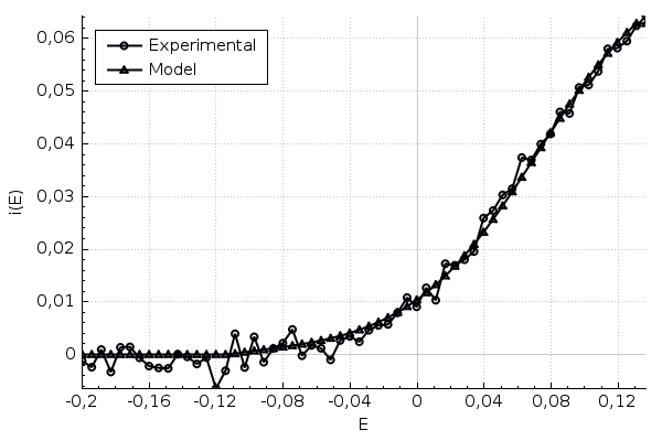
The result of solving of two Inverse Problems for single-component task is presented on Fig.1. We minimized of the cost functional using Hooke and Jeeves algorithm. During the calculations we got one interesting observation: involving in calculations two parameters (instead of one) can sufficiently increase the accuracy of reconstruction. More precisely, we obtained calculation error $3.44\%$ reconstructing only one parameter, and errors $1.05\%$ and $1.6\%$ for two parameters. Moreover, some parameters (for example, $i_{0}$) can be calculated only together with other parameters - our calculation failed while computing only $i_{0}$.

a)	b)

Figure 1: Results of modelling and reconstruction for noised model task, defined in Table 1. On both pictures we use as an experimental curve the result of modelling using the straight solution of (1) with added white additional noise ($10\%$). a) Curve, modelled with special functions after reconstruction of parameter $C_{0}$ only. Calculation error: $3.44\%$. b) Curve, modelled with special functions after reconstruction of parameters $C_{0}$ and $\alpha$. Calculation error: $1.05\%$ and $1.6\%$ for parameters $C_{0}$ and $\alpha$ respectively.

4.3 Double-component model task.

For this test we used enter data (curve), modelled using electrochemical parameters, shown in Table 2.

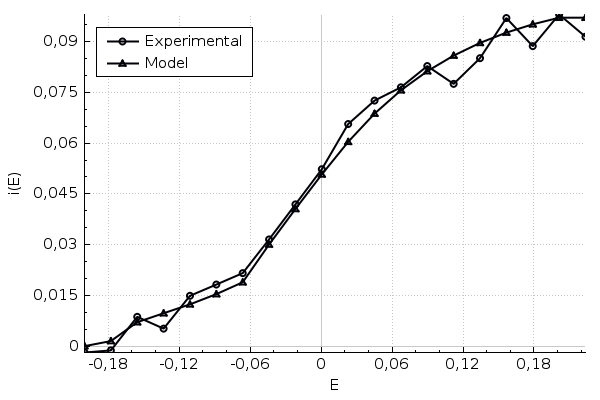
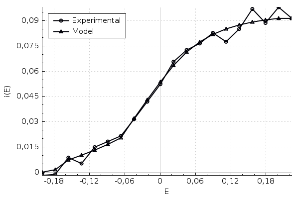
During this calculations we also obtained the same effect: efficiency of calculation of two parameters in time ($C_{0}$ and $\lambda$) is higher in comparison with one-parameter calculation. More precisely, we obtained error $19\%$ and $16.2\%$ respectively, calculating only parameters $C_{0}^{0}$ and $C_{0}^{1}$.

Table 2: Electrochemical parameters for double-component model

Parameter	Values for the first component	Values for the second component
$Z$	2	2
$D$	6.1e-06	6.5e-06
$\alpha$	0.144	0.32
$E_{0}$	-0.18	-0.05
$i^{0}$	0.0064	0.0079

In case, when parameters $\alpha^{k}$ also have being calculated, we obtained errors $3.6\%$ and $6.6\%$ for concentrations $C_{0}^{0}$ and $C_{0}^{1}$ and $14\%$ and $1.2\%$ for transmission numbers $\alpha^{0}$ and $\alpha^{1}$. Enter curve, modelled for this task (with parameters from Table2), and the results of modelling for reconstructed parameters are presented on Fig.2.

a)	b)

Figure 2: Results of modelling and reconstruction for noised model task, defined in Table 2. On both pictures we use as an experimental curve the result of modelling using the straight solution of (1) with added white additional noise ($10\%$). a) Curve, modelled with special functions after reconstruction of parameters $C_{0}^{k}$ only. Calculation errors: $19\%$ and $16.2\%$ for $C_{0}^{0}$ and $C_{0}^{1}$ respectively. b) Curve, modelled with special functions after reconstruction of parameters $C_{0}$ and $\alpha$. Calculation error: $3.6\%$, $6.6\%$ for $C_{0}^{0}$, $C_{0}^{1}$ and $14\%$, $1.2\%$ for $\alpha^{0}$ ,$\alpha^{1}$

4.4 Single-component real task.

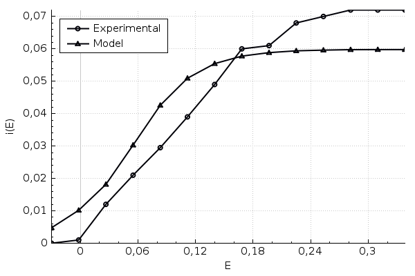
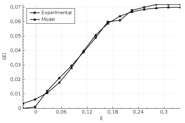
In this subsection we present the results of real voltammeric curve processing. The experimental data are obtained during the voltammetry for Cu electrolyte. All parameters are already presented in Table 1 (above we used these parameters for single-component model task). Because of knowing these parameters, we also can estimate an accuracy of the reconstruction. As above, the accuracy of reconstruction of two parameters is higher than the accuracy of one parameter reconstruction. In first case we obtained an error $19.2\%$ for reconstructed value of concentration $C_{0}$, and $4.6\%$ and $12.2\%$ for parameters $C_{0}$ and $\alpha$ in case of two parameters calculation. Experimental and modelled curves for both cases are presented on Fig.3

a)	b)

Figure 3: Results of reconstruction for real task (parameters in Table 1). a) Curve, modelled with special functions after reconstruction of parameter $C_{0}$ only. Calculation error: $19.2\%$. b) Curve, modelled with special functions after reconstruction of parameters $C_{0}$ and $\alpha$. Calculation error: $4.6\%$, $12.2\%$ for $C_{0}$ and $\alpha$ respectively.

References

- [1] Z.Galus. Fundamentals of Electrochemical Analysis. Ellis Horwood, Chichester, 2 edition, 1994.
- [2] C. Banks R. Compton R. Understanding Voltammetry. Icp, 2 edition, 2010.
- [3] M. Bogdan, D. Brugger, and W. Rosenstiel et al. Estimation of diffusion coefficients from voltammetric signals by support vector and gaussian process regression. J. Cheminform, 6, 2014.
- [4] V.K.Varentsov A.N. Koshev. Description of electrochemical reactions at electrode-electrolyte interface as boundary conditions in case of mathematical simulation of processes in flow 3d electrode. Russian Journal of Electrochemistry, 50(9):846–851, 2014.
- [5] N.Koshev. On the solution of forward and inverse problems ofvoltammetry. Inverse Problems and Applications, Springer Proceedingsin Mathematics & Statistics, 120:153–164, 2015.
- [6] F.Scholz A.Bard, G.Inzelt. Electrochemical Dictionary, volume XVII. Srpinger, 2 edition, 2012.
- [7] A.N. Tikhonov B.M. Budak, A.A.Samarsky. Problem Examples for mathematical physics. Nauka, Moscow, 2015.
- [8] V. M.Klibanov, N. A. Koshev, L.I.Jingzhi, and A. G. Yagola. Numerical solution of an ill-posed cauchy problem for a quasilinear parabolic equation using a carleman weight function. pre-print, 2016. arXiv:1603.00848 [math-ph].
- [9] V.V. Kuzina A.N. Koshev. Modelling and calculation of electro-active component concentration in the process of electrolysis. Large-scale Systems Control, 33:233–253, 2015.
- [10] A. G. Yagola A. N. Tikhonov, A. S. Leonov. Nonlinear ill-posed problems. Chapman & Hall, 1998.
- [11] C.T.Kelley. Iterative Methods for Optimization, volume 18. SIAM, Philadelphia, 1999. Frontiers in Applied Mathematics.
- [12] S.Wright J.Nocedal. Numerical Optimization. Springer Series in Operations Research and Financial Engineering. Sptinger-Verlag, New York, 2006.
- [13] J.W. Thomas. Numerical Partial Differential Equations: Finite Difference Methods. Springer-Verlag, 1995.