page direct0 g
Tensor integrand reduction via Laurent expansion
Abstract
We introduce a new method for the application of one-loop integrand reduction via the Laurent expansion algorithm, as implemented in the public C++ library Ninja. We show how the coefficients of the Laurent expansion can be computed by suitable contractions of the loop numerator tensor with cut-dependent projectors, making it possible to interface Ninja to any one-loop matrix element generator that can provide the components of this tensor. We implemented this technique in the Ninja library and interfaced it to MadLoop, which is part of the public MadGraph5_aMC@NLO framework. We performed a detailed performance study, comparing against other public reduction tools, namely CutTools, Samurai, IREGI, PJFry++ and Golem95. We find that Ninja outperforms traditional integrand reduction in both speed and numerical stability, the latter being on par with that of the tensor integral reduction tool Golem95 which is however more limited and slower than Ninja. We considered many benchmark multi-scale processes of increasing complexity, involving QCD and electro-weak corrections as well as effective non-renormalizable couplings, showing that Ninja’s performance scales well with both the rank and multiplicity of the considered process.
1 Introduction
Scattering amplitudes in quantum field theory describe the fundamental interactions between elementary particles and provide a powerful way for inferring theoretical models form high-energy phenomenology and vice-versa. At the scales probed by modern colliders, such as the Large Hadron Collider (LHC) at CERN, scattering amplitudes can be computed in perturbation theory as a Taylor expansion in the coupling constants. Leading-order results are plagued by very large theoretical uncertainties and as such they are often not reliable enough for direct comparisons with experimental results. Phenomenological studies can significantly benefit from theoretical predictions at next-to-leading order accuracy or beyond, which are however complicated by several factors, a crucial one being represented by quantum corrections to amplitudes computed via loop integrals. The calculation of these integrals can be extremely challenging, especially for processes involving many external legs and physical scales. Such processes can however be of great relevance, both for testing the Standard Model in unexplored regions of phase space and for simulating backgrounds to signals of interesting (new) physics. This makes the calculation of loop amplitudes a very active field of research.
A solution to the problem of computing generic one-loop integrals is offered by integrand reduction [1, 2, 3].
Integrand reduction methods rewrite one-loop integrands as a linear combination of terms in an integrand basis, each of which has five or less loop propagators and yields either a vanishing integral or a known Master Integral. The numerical evaluation of these master integrals is possible by means of public libraries such as OneLOop [4], Golem-95 [5, 6], LoopTools [7] and QCDLoop [8] (the last two use the FF library [9] internally). Because the form of the integrand basis is universal and independent of the process or the number of external legs, the algorithm can be applied to any one-loop scattering amplitude in any Quantum Field Theory. The coefficients of this decomposition, also known as integrand decomposition or OPP decomposition [1], can be efficiently computed by evaluating the integrand on multiple-cuts, i.e. values of the loop momentum such that a subset of the internal loop propagator denominators vanish. This algorithm is based on repeated numerical evaluations of the integrands and the solution of the resulting subsystems of equations for the coefficients. The method has been implemented in the public codes CutTools [10] and Samurai [11], and has been used within several automated frameworks [7, 12, 13, 14, 15, 16, 17, 18, 19] for producing a wide variety of phenomenological results. MadLoop [20], part of the MadGraph5_aMC@NLO [21] framework (abbreviated MG5aMC henceforth), is an example of such tool. It automatically generates one-loop matrix elements and computes them using both traditional OPP reduction (CutTools and Samurai) and tensor integral reduction [22, 23] (as implemented in the tools Golem95 [24], PJFry++ [25] and IREGI). MadLoop features an in-house implementation of the OpenLoops method [16] using a modified version of the ALOHA [26] module to compute the components of the tensor integrand numerator.
More recently, a new approach to one-loop integrand reduction has been developed, namely the integrand reduction via Laurent expansion method [27], which elaborates on techniques first proposed in [28, 29] for analytic calculations. Within this approach, the computation of the coefficients of the Master Integrals is significantly simplified by performing a Laurent expansion of the integrands with respect to the components of the loop momentum which are not constrained by the multiple-cut conditions. Since loop integrands are rational functions of the loop components, within semi-numerical calculations the semi-analytic Laurent expansion can be performed via a simplified polynomial division algorithm between the expansion of the numerator and the loop denominators. Such a technique has been implemented in the public C++ library Ninja [30], which combined to the one-loop package GoSam [15, 31, 32] has been used for producing several phenomenological results for complicated processes both within the Standard Model and beyond.
The Laurent expansion reduction algorithm implemented in Ninja needs as input procedures which return the leading terms of the above mentioned parametric Laurent expansions of the numerator of the integrand. Generating such input is straightforward and easy-to-automate for analytic one-loop generators such as GoSam [15, 31] and FormCalc [7], but it has so far prevented other one-loop tools following a more numerical approach from using reduction via Laurent expansions.
However, as already noted in ref.s [27, 30], the only explicit analytic information needed by Ninja about the integrand is its dependence on the loop momentum (and not, for instance, on the external kinematics or polarization states), which is always known in the case of tensor-based loop generators, regardless of whether the entries of the tensors are generated analytically or numerically.
We present an efficient numerical algorithm for constructing the Laurent expansions needed by Ninja directly from the (numerical) entries of loop tensor numerators. In particular, each term of these expansions can be computed by contracting the tensor numerator with specific cut-dependent tensorial projectors. In a numerical implementation, these projectors can in turn be constructed at run-time by means of simple recursive formulas, from lower to higher ranks. This algorithm has been implemented within the Ninja library and the only inputs it needs for the reduction, besides the definition of the loop propagators, are the numerical components of the tensor numerator. This allowed to interface Ninja to MadLoop whose ability to compute these components is now sufficient, as demonstrated in this paper.
In sect. 2, we recall the definition of the tensor integrand and in sect. 3 we briefly review the integrand reduction technique via Laurent expansion. We fix the notation and introduce the computational techniques for building symmetric tensors in sect. 4 which we use in sect. 5 to derive formulas for the projection of the tensor numerator onto the coefficients of the Laurent expansion. Details on the implementation of this projection in Ninja as well as its interface to MadLoop are provided in sect. 6. We present a detailed study of the stability and timing performances of the combination of MadLoop and Ninja in sect. 7 and we give our conclusions in sect. 8.
2 Tensor integrands
A generic one-loop amplitude can be written as a sum of -point integrals of the form
| (2.1) |
The numerator of the integrand is a polynomial in the components of the -dimensional loop momentum , with , while the denominators correspond to Feynman loop propagators and they have the general quadratic form
| (2.2) |
where is a linear combination of external momenta and is the mass of the particle propagating in the loop (which can be complex-valued when treating unstable particles in the loop within the complex mass scheme [33, 34]). One can split the -dimensional loop momentum into a four-dimensional part and a -dimensional part ,
| (2.3) |
The numerator thus becomes a polynomial in the four-dimensional components of and ,
| (2.4) |
We define a four-dimensional tensor numerator as a numerator cast into the form
| (2.5) |
where the tensor coefficients are independent of the loop momentum. In principle one could consider the more general definition of a -dimensional tensor numerator, i.e. a linear combination of terms with the form of the r.h.s. of Eq. (2.5) multiplied by powers of . Although it is straightforward to generalize the results of this paper to -dimensional numerators, we will only consider the four-dimensional case since tensor-based one-loop matrix element generators typically compute the contributions arising from terms in the numerators (also known as contributions) separately using special tree-level Feynman rules [35].
In the definition in Eq. (2.5), a tensor numerator is therefore defined by a sum of tensors homogeneous in rank , for . The maximum rank satisfies for renormalizable theories, up to a gauge choice. In this paper we will consider a more general case, i.e. , allowing for up to one effective non-renormalizable vertex in the loop.
In a naive implementation, a generic tensor-numerator of rank would be defined by entries, growing exponentially with the rank. However, since the tensor described by Eq. (2.5) is completely symmetric by construction, we can cast the numerator in the alternative form
| (2.6) |
where the total number of -symmetric coefficients for (only defined for ) is now , which only grows polynomially (namely as ) with the rank.
In order to clarify the notation, we consider the following example of an arbitrarily chosen -dimensional numerator function
| (2.7) |
which can be recast into the tensorial structure
| (2.8) |
where denotes the collective kinematic information of the phase-space point considered (external momenta, masses, helicity and color assignation, etc…). The notation indicates that the corresponding tensor components are symmetrized according to the procedure described by Eq. 4.1. The four-dimensional tensor numerator is thus obtained by setting and identifying the Lorentz structures multiplying the loop momentum
| (2.9) |
Several techniques have been proposed for constructing the tensor loop numerator. MadLoop, which features an independent implementation of the OpenLoops method [16], progressively builds the loop numerator polynomial by successive calls to building block functions numerically computing the loop four-momentum dependence of each vertex and propagator involved in the loop. Contrary to analytic methods, this approach makes it very difficult to reconstruct the -dimensional dependence of the loop numerator, so that it is important that the loop reduction algorithm works equally well with only the 4-dimensional projection , in which case the missing rational terms arising from will be reconstructed independently. An alternative method proposed in ref. [19], addressing the case where a numerical evaluation of the integrand is available but its full polynomial structure is not known, reconstructs the entries of the tensor by sampling the numerator on several values of the loop momentum.
In this paper, we will consider a one-loop tensor integrand to be defined by the entries of the symmetric tensor numerator in Eq. (2.6), as well as the momenta and masses appearing in the loop denominators as in Eq. (2.2). Thanks to the new projection techniques introduced in this paper, these are now the only input required by Ninja for performing the corresponding loop reduction.
3 Semi-numerical integrand reduction via Laurent expansion
In this section we briefly review the input needed by the semi-numerical integrand reduction via Laurent expansion algorithm [27] as implemented in the C++ library Ninja [30]. We make no attempt in giving a comprehensive description of this reduction method, which can instead be found in ref.s [27, 30]. Indeed, in this paper we are merely interested in illustrating how to provide the required input starting from a tensor integrand defined as in sect. 2, while the internals of the reduction algorithm are unchanged with respect to what has already been presented in the literature.
Integrand reduction methods compute loop integrals by exploiting the knowledge of the algebraic structure of the respective integrands. In more details, any one-loop integrand in dimensional regularization can be written as a sum of contributions with five or less loop propagators, regardless of the number of external legs or the complexity of the process. The corresponding numerators, also known as residues, are polynomials with a universal, process-independent parametric form. The unknown process-dependent coefficients appearing in this parametrization can thus be found via a polynomial fit. After integration, the amplitude is expressed as a linear combination of known Master Integrals, whose coefficients can be identified with a subset of the coefficients appearing in the integrand decomposition.
An efficient way of computing the coefficients of the integrand decomposition is by evaluating the integrand on multiple cuts, i.e. on values of the loop momentum such that a subset of loop denominators vanish. Indeed, when evaluating the integrand on the generic multiple cut , the only non-vanishing contributions to the integrand decomposition are those coming form the residues sitting on the cut (i.e. vanishing) denominators, as well as from the higher-point residues having the cut denominators as a subset of their propagators. This suggested the possibility of computing the coefficients of each residue by evaluating the integrand on a subset of the solutions of the multiple-cut equations defined by its loop denominators, subtracting the non-vanishing contributions form higher-point residues and solving a system of equations for the unknown coefficients. This is therefore a top-down approach, where higher-point residues are computed first (starting form 5-point residues) and systematically subtracted from the integrand when evaluating lower-point residues. These are known as subtractions at the integrand level. This is the approach followed by the public reduction codes CutTools [10] and Samurai [11].
As we mentioned, the integrand reduction via Laurent expansion method [27] can achieve better stability and performance by exploiting the knowledge of the analytic dependence of the integrand on the loop momentum. More specifically, on top of the numerical evaluation of the loop numerator, the algorithm needs as input a numerical evaluation of the leading terms of the numerator with respect to properly defined Laurent expansions, parametric in the directions of the loop momentum unconstrained by the multiple-cut conditions. From these, the coefficients of the integrand decomposition are computed via a simplified polynomial division algorithm between the expansion of the numerator and the loop denominators and corrected by counter-terms depending on higher-point residues. These are referred to as subtractions at the coefficient level, which simplify and replace the ones at the integrand level of the original algorithm.
In the following we describe the four inputs needed by Ninja, assuming the rank satisfies , while in the next sections we will describe how to automatically generate them at run-time from the coefficients of a tensor numerator. In this section we consider a generic -dependent numerator for the sake of generality, although, as already mentioned, we will later specialize to the case of a four-dimensional tensor numerator defined as in Eq. (2.6). Notice however that the -dependence arising from the expansion of the loop momentum must be considered in both cases. The four input functions are
-
•
the numerator function used for the cut-constructible part of 4-point residues and optional internal tests
(3.1) as a function of the loop momentum (notice that this is the same input as in traditional integrand reduction algorithms),
-
•
the -expansion used for the rational part of 4-point residues, returning the terms defined by the expansion
(3.2) as a function of the four-vectors and
(3.3) -
•
the -expansion used for 3-point and 1-point residues, returning the terms defined by the expansion
(3.4) as a function of the four-vectors and the complex number
(3.5) -
•
the -expansion used for 2-point residues, returning the terms defined by the expansion
(3.6) as a function of the four-vectors and the complex numbers , with
(3.7)
We remind the reader that the vectors defining the expansions are cut-dependent, so that the methods for the corresponding coefficients will be called on all the relevant cuts (and possibly more than once per cut, as needed) within one loop reduction. The terms above are all those needed for calculations with . If the rank is lower than , fewer terms are needed, and in numerical implementations one should take care that only a minimal number of terms is computed so as to optimize performances.
Any one-loop generator capable of providing a numerical evaluation for the terms in Eq. (3.3), (3.5) and (3.7), on top of the evaluation of the numerator as in Eq. (3.1), can use Ninja. We now turn to describing a method for building these expansions from a tensor numerator of the form of (2.6). The algorithm then proceeds in a purely numerical way, using as input only the (numerical) entries of a symmetric tensor numerator. Indeed, as already mentioned, the terms of each expansion (3.2)-(• ‣ 3) can be defined as contractions between the tensor numerator and cut-dependent tensors which Ninja can build at runtime by means of recursive algorithms. Since all the methods defined above have been implemented within the Ninja library for generic tensor integrands with , this allows current one-loop tensor generators to use Ninja for the reduction, simply by providing the coefficients defining the loop numerator as in Eq. (2.6).
4 Symmetric tensors
In this section we introduce some notation on symmetric tensors and recursive formulas useful for efficiently building the cut-dependent tensorial projectors appearing in our results.
4.1 Notation
Consider a set of independent vectors and the symmetrized tensor product of (not necessarily distinct) vectors , with , namely
This tensor, being completely symmetrized, only depends on the number of times each enters the product. As noted in ref. [36], one can exploit this and introduce a natural correspondence between symmetric tensors and polynomials. More in detail, we will use the following polynomial notation
| (4.1) |
where is the multiplicity of occurrence of on the r.h.s. of the equation, with . The conventional prefactor we introduced on the r.h.s. exactly cancels out against the equivalent permutations of the tensor indexes, which turns out to be particularly convenient for our application. This is better clarified with a couple of explicit examples
| (4.2) |
The notation is also useful for writing tensor relations in a compact way.
As a shorthand, if and are symmetric tensors of identical rank , we also define the contraction
| (4.3) |
where the sum over repeated indices is restricted so as to be consistent with the definition in Eq. (2.6).
4.2 Recursive formulas
Tensors can be built recursively by multiplying lower rank tensors with vectors. For this purpose, we can define the tensor product of a rank- tensor with a vector as the rank- tensor
| (4.4) |
Notice that, even if is symmetric, the r.h.s. will in general not be a symmetric tensor. However one can easily work out recursive formulas which build symmetric tensors from linear combinations of tensor products.
The easiest recursive formula involves rank- tensors obtained by multiplying a single vector with itself times, namely
| (4.5) |
The easiest non-trivial case involving two vectors and is
| (4.6) |
The tensor in the first addend on the r.h.s. can in turn be built beforehand using Eq. (4.5), while the tensor appearing in the second addend is instead of the same type of the one on the l.h.s. but with a lower rank. Eq. (4.6) can thus be read as a recursive formula for building symmetric tensors of the form , where the recursion goes from lower to higher ranks , starting from which trivially reads . A useful generalisation of Eq. (4.6) is
| (4.7) |
which should be read as a recursion relation in both and . Indeed, the second addend involves a symmetric tensor which is of the same type as the l.h.s. but with total rank . The tensor in the first addend may instead be rewritten as , with and , hence as a tensor of the same form as the l.h.s. but with lower values of and .
For our purposes we need one more recursive formula involving three vectors , and , which reads
| (4.8) |
The ingredients for this recursion are, similarly as before, tensors with lower and , as well as tensors of the form of Eq. (4.7).
It is also worth observing that all these recursive formulas can be seen as special cases of a more general one
| (4.9) |
An important observation for numerical calculations is that these recursive formulas have the nice side effect of automatically embedding a system of abbreviations based on reusing common subexpressions. Indeed, as one can see from the definition in Eq. (4.4), each entry in a tensor product of total rank can be obtained from an entry of rank by a single multiplication. Because our formulas are recursive on the rank and involve linear combinations of tensor products, they provide a built-in mechanism for reusing subexpressions of lower rank when building tensors of higher rank. Moreover, the possibility of reusing common subexpressions is not limited to contributions defined within the same recursive formula, but it can also be extended to contributions across different equations in a way which fits particularly well with the method we will use for building the Laurent expansions of the integrands. We will see in the next section that the leading term of a Laurent expansion can always be obtained from tensors of the form of Eq. (4.5). Next-to-leading terms, when needed, will be constructed using Eq. (4.6). As we already observed, the r.h.s. of this equation involves a lower-rank tensor of the same form as the l.h.s. and a tensor of the same form of Eq. (4.5). While the former is available simply by implementing the recursion from lower to higher ranks, the latter can instead be reused from the tensors recursively built for the leading term. An analogous strategy is also possible for Laurent expansion terms beyond next-to-leading, where one can always use tensors built in previous steps of the calculation as input for the recursive formulas (more explicit examples will be given in sect. 5). This greatly reduces the total number of operations needed for the construction of these tensors, without hard-coding complex analytic formulas and while having a relatively simple bookkeeping and still being completely general with respect to the rank of the tensors appearing in the recursion relations.
5 Tensor projectors for Laurent-expansion terms
As we stated above, we can build the terms of the Laurent expansions described in sect. 3 by contracting the tensor numerator with appropriate cut-dependent tensors, which can be seen as projectors. These can in turn be built recursively using the formulas of sect. 4.2. We will illustrate the method by explicitly working out a few cases. A complete list of formulas for all the tensor projectors is given in Appendix A.
As stated above, in the following we will consider a four-dimensional tensor numerator defined as in Eq. (2.6), which thus only depends on the four-dimensional components of the loop momentum. However, because Ninja implements a -dimensional version of the integrand reduction method, the parametrization of on the -dimensional cut solutions (and thus its Laurent expansion) will still depend on the extra-dimensional variable and we must therefore keep track of this dependence while building the expansions (knowing, of course, that it can only come from the loop momentum, and not from the numerator). This -dimensional reduction yields, on top of the coefficients of the master integrals, the contributions to the rational part of the amplitude coming from the dependence of the loop denominators, also known as . An alternative approach to the calculation of (used for instance by CutTools) is its reconstruction from the coefficients of a purely four-dimensional reduction, also known as cut-constructible part. It is worth stressing that, as one can observe from the results collected in Appendix A, the calculation of the Laurent expansion terms involving , with the approach presented in this paper, can always be recycled from the identical terms needed for the cut-constructible part, except for the box residues where the expression is however very simple. This allows to efficiently provide the algorithm of Ninja with all the terms needed by its -dimensional integrand reduction, while remaining completely agnostic about the -dependence of the loop numerator within the reduction routines.
In the following, is the number of loop propagators and is the rank of the tensor numerator. The Laurent-expansion parameter is denoted by , and it is always convenient to compute the terms from higher to lower powers of . A first reason for this is that the highest powers of are always needed, while the lower powers might not be. A second compelling reason is that, as we already mentioned, tensors built for the leading terms in can be reused as input for building terms with lower powers of , using the recursive formulas introduced in the previous section.
5.1 Numerator evaluation
The easiest function to provide is the evaluation of the numerator function which, using Eq. (2.5), simply amounts to
| (5.1) |
where we used the notation introduced in sect. 4 (in particular Eq. (4.1) and (4.3)). Each tensor can in turn be built using the recursive formula of Eq. (4.5), which here reads
| (5.2) |
5.2 The -expansion
The -expansion, only needed for , involves a single term for and two terms for . Since the vector comes with a power of , while is , it is straightforward to see that the leading term in of the expansion defined by Eq. (3.2) is
| (5.3) |
As done before, we can build recursively by means of Eq. (4.5)
| (5.4) |
For the case where , we also need the next-to-leading term in , which is given by the following formula
| (5.5) |
where the tensor appearing in the first addend of the r.h.s. was already built for the leading terms using Eq. (5.4), while for the second addend we can use the recursive relation in Eq. (4.6), which in this case reads
| (5.6) |
The first addend of this recursive relation also depends on tensors built using Eq. (5.4) for the leading term, while the second depends on a lower-rank tensor which gives the recursion in .
5.3 The -expansion
The -expansion has a more complicated structure due to the presence of three vectors (, and ) and the free variable on top of the expansion variable . More in detail, the vector comes with a power of , the vector is and the vector has a term multiplied by the constant and a term. Hence, the projector for the leading term is a tensor containing only , while replacing a by a decreases the power in by one, and replacing a by a decreases the power in by two and also adds a term.
Since the leading and next-to-leading terms of the expansion do not involve (and thus neither ), they have exactly the same structure as those for the -expansion. They are
| (5.7) |
and
| (5.8) |
The next-to-next-to-leading terms in are two, namely a term and a term, and their expression involves all the three vectors , and . They are given by the following formulas
| (5.9) | ||||
| (5.10) |
It is worth making a few observations. We already mentioned that the -dependent terms can be determined from the cut-constructible ones, and indeed the contribution is common between the two equations and thus only needs to be computed once. Moreover the tensor , and more in general all those of the form , can be computed from the recursion relation in of Eq. (4.5) which in this case depends on the tensors already computed above for the leading term in . The tensor can instead be computed using the formula in Eq. (4.7) with , to be read as a recursion relation in and depending on tensors of the form already computed for the next-to-leading terms in .
Similarly, one can compute all the other terms with lower powers of , by means of a simple power counting on the vectors , and , and building appropriate tensors with the formulas of sect. 4.2. One can also check that the formulas of Eq. (4.5), (4.7) and (4.8) suffice for the calculation of all the terms down to , which is all one needs for integrands with . At each step one can perform the recursion with respect to , for , reusing as ingredients tensors computed for lower or for terms with higher powers of . Explicit formulas for all terms are given in Appendix A.
5.4 The -expansion
The terms for the -expansion can be computed using the same method as for the -expansion. Since we are now dealing with three variables (, and ) and four independent vectors (, with ) the main difference is a more involved bookkeeping, partially mitigated by the need of less powers in . Explicit formulas are collected in Appendix A.
6 Implementation
The tensor projectors for the Laurent expansion terms described above have been implemented in the Ninja library.
The reduction algorithm implemented in Ninja requires as input a numerator which is an abstract interface implementing the methods described in sect. 3 (the C++ programming interface is described in ref. [30]). We thus implemented such an interface which computes the expansion terms collected in Appendix A from the coefficients of a generic tensor numerator, defined according to Eq. (2.6).
The tensor numerator is treated as a polynomial whose coefficients are stored in a unidimensional array, from lowest to highest according to the graded lexicographic monomial order in the variables with (i.e. terms are ordered by their total degree and terms with the same total degree are ordered lexicographically). This is the same monomial order used internally by MadLoop and turns out to be particularly convenient for building the tensors described in this paper, since we use formulas which are recursive with respect to the total rank. It is worth observing however that none of the results presented in this paper rely on a specific representation of the momenta (and consequently of the tensor numerator). In particular, the formulas collected in Appendix A, as well as the algorithms implemented for building the corresponding tensors, are unchanged after a change of coordinates and can thus be applied to any other representation of the four-dimensional components after converting the momenta used as input into the alternative representation.
We also implemented in Ninja a Fortran-90 wrapper exposing this tensor interface, which in principle can be used by any one-loop tensor-based generator by specifying the loop propagators and the coefficients of the tensor numerator defining the integral to be computed. Both the Fortran and the C++ interface are publicly available since version 1.1.0 of the library.
MG5aMC (v2.3.4 and onwards) now includes a version of Ninja which is used as the default loop reduction method111Other alternative reduction algorithms (CutTools, PJFry++, Golem95, IREGI and Samurai) are still used in the event that MadLoop stability tests deem the kinematic configuration numerically unstable.. This default installation of Ninja can be automatically updated to the latest online one (independently distributed) by running the following command in the MG5aMC interactive interface:
MG5_aMC> install ninja
Ninja, similarly to CutTools is available both in double and quadruple precision at runtime and MadLoop will dynamically switch to quadruple precision when its internal stability tests indicate that the double precision computation does not meet the requirement in numerical accuracy. In MadLoop, the computation of the tensor numerator coefficients is completely independent from the loop reduction and, as a result, the stability rescue is first attempted by re-performing in quadruple precision only the loop reduction (although with input kinematics already promoted to quadruple precision accuracy). This is often enough to restore satisfactory numerical stability, hence avoiding the much more time-consuming full-fledged quadruple precision computation.
We also point out that Ninja’s internal kinematic matrix , with quantities defined as in Eq. (2.2), is initialized directly in MadLoop where the following three on-shell limits are set to be exact when below a certain adimensional threshold set to by default:
-
•
If , set if
-
•
If , set if
This proved to help the numerical stability of the reduction, essentially because it avoids ever approaching the kinematic region where the master integrals switch from a massive to massless description. The choice of the analytic expression to be evaluated by the Master Integral library is typically controlled by an internal infra-red threshold parameter which would apply to each integral independently. By regulating the kinematic matrix in MadLoop, we guarantee the consistency of the expression employed for all master integrals.
Finally, all loop reduction methods except CutTools and IREGI can be independently (de-)activated before the generation of the one-loop matrix element numerical code by setting the corresponding MG5aMC path options in <MG_root>/input/mg5_configuration.txt. If activated at generation time, then their use at run time can be controlled via the parameter MLReductionLib specified in the file MadLoopParams.dat.
7 Applications
In this section, we will present the summary of a detailed study of the timing and stability performances of MadLoop interfaced to Ninja. When available, we compare the results obtained with Ninja against other reduction algorithms, namely CutTools, Samurai, IREGI, PJFry++and Golem95, whose limitations (for the versions interfaced to MadLoop) are summarized in table 1. CutTools is a library implementing a four-dimensional version of the integrand reduction method, as well as a reconstruction of the term as explained at the beginning of section 5. Samurai is a similar tool which always performs a full -dimensional integrand reduction, making it capable of handling -dimensional loop numerators at the price of being less efficient of four-dimensional ones, since it implements a more complex reconstruction of the integrand. IREGI, PJFry++and Golem95 are instead tensor integral reduction tools.
| Reduction tool | Max. | Max. rank |
|---|---|---|
| Ninja | unlimited | |
| Samurai | unlimited⋆ | |
| CutTools | unlimited⋆ | |
| IREGI | 7 | |
| PJFry | ||
| Golem95 | ||
| ⋆: For reducing loops with 9 (11) loop lines and more, Samurai (CutTools) must be recompiled | ||
| with an increased value for its default maximum number of denominators. | ||
| †: Loops with rank are supported in CutTools only for models with effective | ||
| interactions involving only the Lorentz structures of the Higgs-gluons vertices. | ||
| ⋆⋆: This IREGI limitation stems from the observation that its reduction of loops with rank | ||
| larger than 6 is typically unstable for all kinematic configurations. | ||
We stress that MadLoop can dynamically change at run time the active reduction tool depending on its applicability to each individual (group of) loop(s) being reduced.
The study carried in this section focuses on the following five classes of processes, chosen for their different characteristics that cover a wide spectrum of one-loop matrix-element computations. The notation denotes that we considered all the processes with either or occurrences of particle in the final states.
-
•
A)
This class of processes is a common benchmark for pure QCD computations as it introduces the top mass as an additional scale. The one-loop amplitudes for each multiplicity of this class of processes were first computed in ref.s [37, 38, 39]. The one-loop matrix element for the process is generated and computed here for the first time for specific kinematic configurations (see Appendix. D.1). -
•
B)
These processes are computed within the Higgs Effective Interaction Theory as implemented in [40]. In this effective theory the top-quark loop is integrated out, yielding effective interactions between gluons and the Higgs. The resulting dimension-5 operators lead to loops with rank which are especially challenging to reduce. Thanks to the trivial Lorentz structure of the effective Higgs interactions, both CutTools and older versions of Samurai are applicable [27], even though they do no support completely general tensor numerators of higher rank. The one-loop amplitudes for each multiplicity of this class of processes were first computed in ref.s [41, 42, 43]. -
•
C)
This set of processes is similar to the one above, but involving a spin-2 particle of mass 1 TeV and whose graviton-like effective interactions are described in sect. 2.3 of ref. [40] (we considered ). In this case, the tensor numerator of the resulting loops with rank can have an arbitrary structure that CutTools cannot handle. The one-loop amplitudes for this class of processes were first computed in [44] and [45] for 0 and 1 additional gluon in the final states and are computed here for the first time for 2 and 3 additional gluons (see Appendix. D.2). The study of the phenomenology of QCD corrections within this effective theory featuring a spin-2 particle is in preparation [46]. -
•
D)
This is a class of loop-induced processes for which event generation has recently been automated in MG5aMC [47]. Loop-induced processes are processes without any contribution from tree-level Feynman diagrams, in which case the one-loop amplitude must be squared against itself. This implies that when using integrand reduction (and only then), loops must be reduced individually and independently for each helicity configuration.Also, given the absence of any Born contribution, loop-induced processes are finite and build by themselves the complete Leading-Order (LO) prediction. For this reason, the speed of event generation and phase-space integration is entirely driven by the one of the one-loop matrix element, making optimizations especially relevant in this case. The gluon-fusion amplitude for was first computed in [48] and results for the processes and were shown in [49, 47], while the loop-induced processes with four and five final state Z-bosons have never been studied.
-
•
E) , , and
This less uniform class of process with initial states serves different purposes. The first process is intended to be compared with its loop-induced counterpart. The second one includes both EW and QCD loop contributions, of all coupling orders, and it probes the behavior of the loop reduction algorithms in the presence of many scales and with complex masses in the loop propagators. The last two processes test the reduction for high multiplicity processes featuring loops with a large number of loop propagators (up to nine222Note that contrary to Ninja, for enneagons and above Samurai must be recompiled after its hard-coded limit on the number of propagators has been increased.) but low rank. These four high multiplicity processes have been selected for their specific characteristics from the standpoint of loop reduction and they have no direct phenomenological relevance except for the second one, so that their computation is not present in the literature.
The b-quarks are considered massive in all SM processes except for .
7.1 Timing profile
For all processes listed at the beginning of this section, we measure independently the time spent for the computation of the tensor components333This timing profile was performed prior to an optimization in the computation of the tensor numerator (filtering out some tensor components which are analytically zero) which brings a minor improvement on of order (30%) (process dependent). Note that, this does not affect the key comparison of the reduction time between different reduction algorithms. of the loop numerator () and the reduction of the loops (), for one random kinematic and helicity configuration summed over color assignations. We stress that includes the time spent in evaluating the master integrals as well as in the computation of the coefficients of the Laurent expansion in the case of Ninja.
In MadLoop, there is no optimization in the computation of the loop integrand tensor numerator across helicity configurations, so that scales linearly with the number of non-vanishing helicity configurations. Conversely, remains independent of that number since the summation over helicity configurations can be performed before the loop reduction (except for loop-induced processes when using integrand reduction techniques).
We stress that the timing profile for a single helicity configuration is the relevant figure of merit for applications within MG5aMC which does not explicitly sum over helicity configurations for loop contributions, but instead adopts a Monte-Carlo procedure coupled with an adaptive importance sampling.
We summarize our findings in fig. 1 showing results obtained with MadLoop interfaced to either Ninja, Samurai or CutTools.
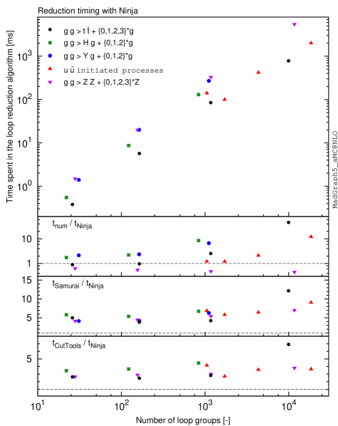
The x-axis registers the number of loop groups which combines all loops that can be reduced together. This corresponds to the set of loops sharing the same topology (i.e. ordered list of loop propagators), except for loop-induced processes where each loop must be reduced individually and therefore lies in a loop group of its own. Notice that since loops identical up to couplings (like fermion loops of different flavors) are combined already when generating the loop matrix element code, they only count as one.
The main feature of the upper panel of fig. 1 is that within each class of processes, the dependence of the reduction time w.r.t. the number of loop groups is linear, as already noticed in [16]. The offset between each class of process is related to the difference in the rank of the constituting loops. The loop rank is typically larger in processes within models with higher dimensional operators (blue hexagons and green squares) as well as in loop-induced processes which involve fermionic loops only (purple triangles). Conversely, the rank becomes smaller as the number of external fermion lines increases and we indeed observe that the timings for the processes and sit on a line underneath (black circles and red triangles). It is interesting to note that that the process is almost two orders of magnitude faster than its loop-induced counterpart, even though they are both contributions to the same final state.
The second inset of fig. 1 shows the ratio of the time spent in the computation of the components of the tensor numerator with the loop reduction time with Ninja. This ratio rapidly increases with the multiplicity and number of loop groups, clearly establishing that within the MadLoop+Ninja implementation, the computation time is asymptotically dominated by the computation of the loop integrand numerator. When no loop grouping is possible, as it is the case for loop-induced processes, we observe the opposite asymptotic behavior hence showing the the loop grouping plays an essential role in this limit. We remind the reader that these conclusions apply to the computation of the loop matrix element for a single helicity configuration and only in the context of MadLoop’s technique for the computation of the loop integrand, which is most flexible but less optimal than full-fledged recursion relations [50], especially for processes with large multiplicity.
The bottom two insets of fig. 1 compare the performances of the three integrand reduction techniques interfaced to MadLoop and reveals that Ninja is about 3 to 5 times faster than CutTools and 5 to 10 times faster than Samurai. The reduction time relative to Ninja increases with the process multiplicity, hence assessing the impact of the advantages of the integrand reduction via the Laurent expansion method as the complexity of the considered processes increases.
7.2 Stability study
We now turn to the assessment of the numerical stability of Ninja for the benchmark processes A)-D) listed at the beginning of this section. We do so by applying the internal stability tests of MadLoop to a set of random kinematic configurations and we report the resulting accuracy as a cumulative distribution for the fraction of points with a reduction relative accuracy larger than some target on the x-axis.
For the processes, we chose to be 100K for =2, 10K for =3 and 1K for 3. These kinematic configurations are chosen randomly, with the constraint that all final states satisfy GeV with angular separation . The center of mass energy chosen is TeV, except for the processes involving the spin-2 particle in which case the center-of-mass energy is set to TeV.
MadLoop combines two stability tests to estimate the numerical accuracy of the result:
-
•
Loop direction test: The loop reduction is performed a second time with the order of all propagators reversed (corresponding to the loop momentum redefinition ) and compared to the original evaluation. This changes the internal numerics of the reduction, hence assessing its stability. Given that the input kinematics remains unchanged, the tensor numerator components do not have to be recomputed.
-
•
Lorentz test: The input kinematic is transformed by a Lorentz rotation for which the loop-matrix element is recomputed and compared to the original one.
Another commonly-used kind of stability test consists in rescaling all dimensionful quantities by a common factor. This is not used by MadLoop because it proves to be impractical in the general case where the dimension of each of the model input parameters is not necessarily available within the generated code.
The stability tests are performed on a computation of the loop matrix element summed over all helicity configurations, except for the loop-induced processes for which only the all-minus helicity configuration is considered.
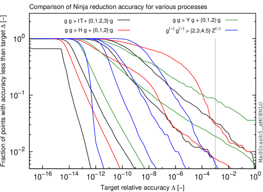
The vertical gray line at (i.e. 3 stable digits) marks the typical threshold used for Monte-Carlo event generation during which MadLoop will attempt to rescue the phase-space points with a numerical stability estimate larger than this target by repeating the reduction (and possibly the computation of the tensor numerator) in quadruple precision. The crossing of the various curves with this gray line therefore gives the fraction of unstable kinematic configurations for which this rescuing procedure will be necessary. For all the processes of highest multiplicity in each class A)-D), this fraction is larger than 1% and almost 10% for , which shows that numerical stability becomes an important issue444Faster and more flexible rescue mechanisms may be obtained using expansions around unstable kinematics, as implemented in the private tool COLLIER [51, 52]. when attempting the integration of processes with loops of rank 6 and especially 7.
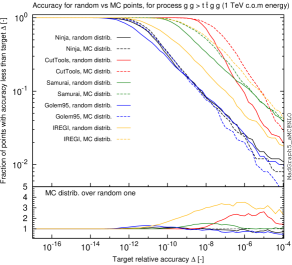
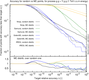
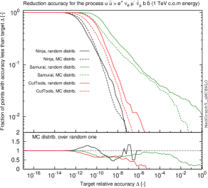
Fig. 3 compares the stability of all applicable reduction tools for the processes , and . We observe that Ninja is always the most stable reduction, comparable to that of Golem95 which is however considerably slower (see appendix B).
In fig. 2, comparing the relative position of the curves for processes with equal number of external legs shows that the determining factor for stability is the tensor numerator rank. This is also manifest when observing that despite the large multiplicity of the process and the complexity of its contributing QCD and EW loops, the stability of its reduction is comparable to that of other processes with a maximum rank of 4.
In an actual Monte-Carlo integration, the phase-space points encountered are not uniformly distributed and as a result the stability profile can potentially be different in this context. For this reason, we also show the stability profiles obtained by considering the kinematics of unweighted events generated at LO accuracy for the LHC14 collider setup using the NNPDF 2.3 (NLO) PDF set [53]. Except for IREGI, we find no qualitative difference and the Monte-Carlo distributions even tend to be slightly more stable for Ninja, showing that its reduction is mainly insensitive to a change of reference frame and c.o.m energy.
In appendix C, we show the stability profiles of processes A)-D) for all applicable reduction tools. These further establish the observations drawn in this section.
8 Conclusions
We presented an algorithm for the generation of the expansion terms needed by the one-loop integrand reduction via Laurent expansion implemented in the public library Ninja from the numerical components of a tensor numerator. We have shown how, within a numerical calculation, these expansion terms can be obtained by contracting the tensor numerator with appropriate cut-dependent tensors, which in turn can be efficiently built by means of simple recursive relations.
The algorithm has been implemented in the most recent version of the public library Ninja, which can thus be used by tensor-based one-loop generators by providing the numerical entries of the tensor numerator of an integral. We interfaced this library to the MadLoop generator, part of the MadGraph5_aMC@NLO framework (available from v2.3.4 onward).
This allowed us to extensively study the performance and the numerical stability of Ninja and compare it with several other available tools. In terms of reduction speed, we observe that Ninja outperforms all other reduction tools, and in particular Samurai and CutTools by a factor of about 6 and 3 respectively. Also, Ninja’s improvement over other tools increases with the complexity of the process. In terms of reduction stability, Ninja improves on previous integrand reduction techniques by a considerable amount and in general stands on par with tensor integral reduction as implemented in Golem95, which is however more limited and significantly slower. Our results show that numerical instability with Ninja only becomes problematic, because of the slowdown induced by reprocessing unstable points using quadruple precision arithmetics, for loop numerators of rank 7 and above which are not of immediate concern for current phenomenology at particle colliders.
The algorithm and the results presented in this paper therefore enhance the capabilities of MadLoop and the applicability of Ninja, and will thus be valuable for future high-energy phenomenological studies, especially those involving amplitudes featuring loop diagrams characterized by loop numerators of high rank.
Acknowledgments
We would like to thank Simon Badger, Pierpaolo Mastrolia, Giovanni Ossola, Stefano Frixione and Fabio Maltoni for useful discussions and comments on the draft, and Goutam Das and Huasheng Shao for their feedback on the use of the interface discussed in this paper. The work of TP is supported by an STFC Rutherford Grant ST/M004104/1 and the work of VH is supported by the SNF grant PBELP2 146525.
Appendix A Explicit formulas for expansion terms
In this appendix we collect all the formulas for the Laurent expansion terms defined in sect. 3. The results have been obtained as described in sect. 5 and implemented in the Ninja library. One can check that all the tensors appearing in the following formulas can be built by means of the recursive relations in Eq. (4.5), (4.7) and (4.8). It is worth observing that, for efficiency reasons, in the actual implementation only a minmal set of terms is computed depending on the cut and on the rank of the numerator. We also make sure to reuse contributions to different terms within the same expansion whenever this is possible.
In the following, we again use the notation introduced in sect. 4.1, with the labeling of the terms in each expansion as defined in sect. 3. Here is the full list of contributions:
-
•
evaluation of numerator
(A.1) -
•
-expansion
(A.2) (A.3) -
•
-expansion
(A.4) (A.5) (A.6) (A.7) (A.8) (A.9) (A.10) (A.11) (A.12) -
•
-expansion
(A.13) (A.14) (A.15) (A.16) (A.17) (A.18) (A.19) (A.20) (A.21) (A.22) (A.23) (A.24) (A.25)
Appendix B Details of timing performances
This section presents MadLoop timing profile for the generation and the computation of the tensor numerator components for all the benchmark processes A)-D) introduced at the beginning of sect. 7. We also show the time necessary for performing the loop reduction with each of the six reduction tools interfaced to MadLoop (when available): IREGI, PJFry++, Golem95, CutTools, Samurai and Ninja. The reader can easily reproduce analogous results for various compilers and machines by using the automated check timing command of the MG5aMC interface.
| Timing profile | ||||
|---|---|---|---|---|
| Generation time | 45 min | 2h10m | 16 min | 2 days |
| # Loop diagrams | 3870 | 51363 | 5875 | 99981 |
| # Loop groups | 1051 | 4343 | 1716 | 18469 |
| Maximum numerator rank | 6 | 4 | 4 | 5 |
| Integrand computation time | 0.17 s | 0.88 s | 0.12 s | 24 s |
| Ninja reduction time | 0.14 s | 0.42 s | 0.10 s | 2.0 s |
| Samurai reduction time | 0.96 s | 2.7 s | 0.58 s | 18.1 s |
| CutTools reduction time | 0.58 s | 1.5 s | 0.27 s | 7.3 s |
| Generation time | 15.6 s | 110 s | 26 min | 29 h |
| # Loop diagrams | 28 | 156 | 1176 | 11700 |
| # Loop groups | 28 | 156 | 1176 | 11700 |
| Maximum numerator rank | 4 | 5 | 6 | 7 |
| Integrand computation time | 0.95 ms | 11 ms | 0.17 s | 2.5 s |
| Ninja reduction time | 1.5 ms | 20 ms | 0.32 s | 5.5 s |
| Samurai reduction time | 6.3 ms | 90 ms | 1.8 s | 39 s |
| CutTools reduction time | 4.0 ms | 58 ms | 1.1 s | 21 s |
| IREGI reduction time | 31 ms | 1.9 s | 120 s | N/A |
| Golem95 reduction time | 20 ms | 0.94 s | 28 s | N/A |
| PJFry++ reduction time | 5 ms | 0.36 s | N/A | N/A |
| Timing profile | ||||
| Generation time | 14 s | 46 s | 14 min | 2 days |
| # Loop diagrams | 36 | 427 | 5547 | 82470 |
| # Loop groups | 26 | 164 | 1168 | 9940 |
| Maximum numerator rank | 3 | 4 | 5 | 6 |
| Integrand computation time | 0.34 ms | 5.5 ms | 215 ms | 36 s |
| Ninja reduction time | 0.38 ms | 5.7 ms | 85 ms | 0.78 s |
| Samurai reduction time | 1.9 ms | 22 ms | 362 ms | 9.5 s |
| CutTools reduction time | 1.0 ms | 14 ms | 240 ms | 5.4 s |
| IREGI reduction time | 5.5 ms | 290 ms | 12.8 s | 13 min |
| Golem95 reduction time | 4.6 ms | 113 ms | 3.4 s | N/A |
| PJFry++ reduction time | 1.1 ms | 50 ms | N/A | N/A |
| Generation time | 28 s | 122 s | 1h50m | |
| # Loop diagrams | 69 | 875 | 12300 | |
| # Loop groups | 22 | 122 | 836 | |
| Maximum numerator rank | 5 | 6 | 7 | |
| Integrand computation time | 0.96 ms | 19.2 ms | 1.1 s | |
| Ninja reduction time | 0.55 ms | 8.7 ms | 130 ms | |
| Samurai reduction time | 3.2 ms | 47 ms | 876 ms | |
| CutTools reduction time | 1.9 ms | 32 ms | 580 ms | |
| IREGI reduction time | 18.6 ms | 1.7 s | N/A | |
| Golem95 reduction time | 6.9 ms | 0.28 s | N/A | |
| Generation time | 72 s | 234 s | 3h20m | |
| # Loop diagrams | 141 | 1463 | 18420 | |
| # Loop groups | 31 | 163 | 1111 | |
| Maximum numerator rank | 5 | 6 | 7 | |
| Integrand computation time | 3.0 ms | 47 ms | 1.8 s | |
| Ninja reduction time | 1.4 ms | 20 ms | 0.27 s | |
| Samurai reduction time | 5.8 ms | 85 ms | 1.7 s | |
| IREGI reduction time | 35.4 ms | 3.5 s | N/A | |
| Golem95 reduction time | 12.5 ms | 0.50 s | N/A |
The numbers shown in tables 2 and 3 refer to the computation of the loop matrix element averaged and summed over color assignments but for a single helicity and kinematic configuration. This is the relevant figure of merit in MG5aMC since it implements a Monte-Carlo over helicity (with importance sampling) when integrating loop contributions. It is worth noting however that for loop matrix elements with a Born contribution, only the numerator computation time () scales with the number of contributing (analytically non-zero) helicity configurations () whereas the reduction time () remains constant as the integrand numerators can be summed over helicity configurations before being reduced. The total time for the computation of the loop matrix element summed over all helicity configurations can therefore simply be computed as
| (B.1) |
since MadLoop does not implement optimizations across different helicity configurations.
For loop-induced processes however [47], this is not possible when using reduction at the integrand level, in which case both and scale with .
The number of loop diagrams indicated does not count the multiple copies with different quark flavors in the loop. A loop group refers to a group of loops which can be reduced together. This number is equal to the number of loops for loop-induced processes since each loop must be reduced individually in this case; otherwise it regroups all loops sharing the same topology (ordered list of denominators identified by their mass and four-momentum flows ).
The synthetic fig. 1 of the main text illustrates best the results and we find that Ninja outperforms all reduction tools considered for all the benchmark processes. We note however that the advantageous apparent exponential growth of the integrand reduction time with the process multiplicity is mitigated by the factorial growth of the time spent in computing the numerator tensor components. This is intrinsic to MadLoop’s approach based on Feynman diagrams which offers maximal flexibility at the expense of not taking advantage of the optimal scaling behavior of recursion relations [50]. We stress that MadLoop implements a caching system for recycling part of trees and loops shared across different diagrams. This emulates what recursion relations achieve, but only to a lesser extent even though it already considerably improves the computation time of the tensor numerator.
Generation time is usually not considered as relevant given that it must be performed once per process only. In practice however, this can be of concern since it is typically not easily parallelizable and is also a general hinderance when it comes to testing, debugging or quickly exploring the impact of some modifications to a model. In MadLoop’s approach, generation time is hardly an issue for current phenomenologically relevant processes, but its growth is such that we reached the limit of reasonable process generation for which requires about 2 days of sequential runtime and 40 GB of RAM.
Appendix C Details of stability performances
In this appendix, we present the stability profiles obtained for processes A)-D) described at the beginning of sect. 7 and for the six loop reductions tools interfaced to MadLoop (when available): IREGI, PJFry++, Golem95, CutTools, Samurai and Ninja. The reader can easily reproduce these profiles by using the automated check stability command of the MG5aMC interface.
Fig. 4 shows results for the process . The plateau displayed by PJFry++ in is reminiscent of a known issue in this tool which is now no longer maintained.
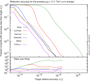
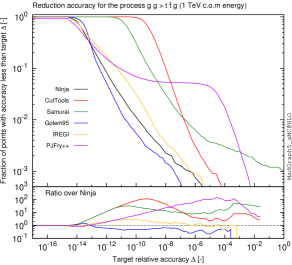
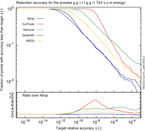
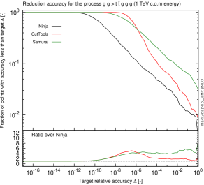
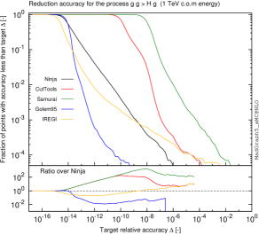
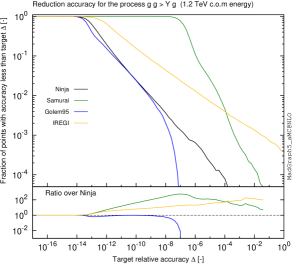
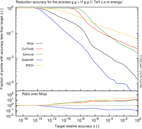
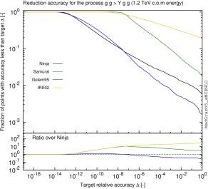
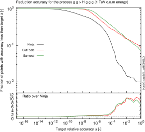
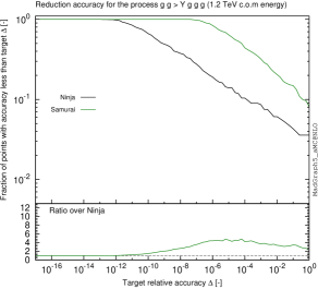
Fig. 5 shows results obtained for the processes involving effective interactions yielding loops of numerator ranks equal to one plus the number of loop denominators. Such loops are particularly challenging to reduce and we observe that the accuracy deteriorates significantly when assuming a completely general form of the higher rank tensor, as it is the case in , compared to the simpler tensor numerators obtained in . Indeed, the residues and consequently the fitting procedure are considerably more involved for higher rank integrands. It is worth noticing that for the simpler tensor structure of however, the Laurent expansion method is significantly more accurate than other integrand reduction tools, since the numerator expansion methods will return zeroes for vanishing higher rank coefficients, thus avoiding the (inexact) numerical reconstruction of such zeroes from multiple evaluations of the integrand. In the Higgs case, the stability profile exhibits an unusual shape with a very steep dependence with in the region , indicating that any decrease of the default Monte-Carlo stability threshold of would have a significant impact on runtime performances as the fraction of points that must be reprocessed using quadruple arithmetics increases. The comparison of the two profiles obtained using tensor integral reduction highlights the importance of the internal numerical stabilization mechanisms of Golem95 as the rank of the loop numerator increases.
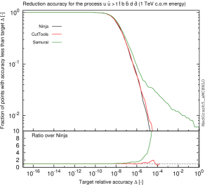
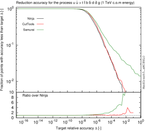
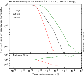
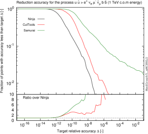
Fig. 6 shows stability results for processes with high multiplicity but relatively low rank. We observe that even though the processes involve up to 8-(9-)loops, their numerical stability is only slightly worse than that of the lower multiplicity processes with equal maximum rank, such as . It is interesting to note that when the multiplicity is larger than the rank by several units, the numerical stability of CutTools and Ninja is almost identical, as expected from the fact that the integrand reduction via Laurent expansion method and the traditional OPP numerator fitting are very similar in this limit. Indeed, when the multiplicity of the loop lines and the rank of the numerator satisfy , one can easily show that the result is only determined by the cut-constructible coefficients of the boxes. These in turn, given their simplicity, are the only coefficients that Ninja computes with the same algorithm as traditional integrand reduction.
The two processes of the bottom insets of fig. 6 introduce new scales in the loop amplitudes; first with external massive lines for for which CutTools is slightly more stable than Ninja (unlike for all other processes) and secondly with internal (complex) massive lines for the complete QCD+EW loop contributions to the process for which Ninja is more stable.
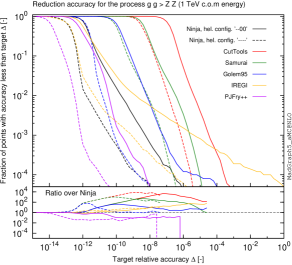
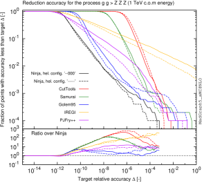
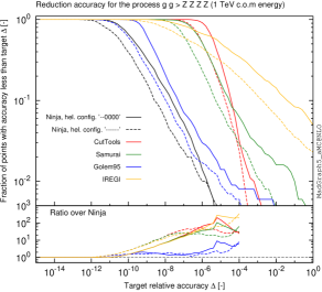
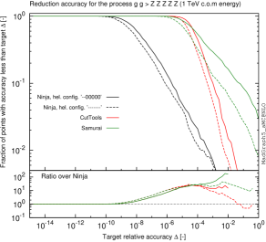
From the numerical stability standpoint, the interesting characteristics of loop-induced processes such as is that they only involve fermion loops of maximal numerator rank. Contrary to the stability studies performed on all other classes of processes, we investigated the loop-induced ones by considering only a single helicity configuration; either (all-minus) or (all longitudinal Z bosons). We find a similar stability behavior for both helicity configurations, except for the lowest multiplicity process.
The peculiarity of the process is that its fermion box loop contribution becomes unstable when the transverse momentum of the final state -bosons tends to zero (i.e. all external momenta aligned on the beam axis). Given the constrained kinematics, this configuration is often probed which is also why this process is typically integrated using a technical (very) small cut in the -boson . The upper left plot of fig. 7 reveals that in this limit, the fermion box stability significantly depends on the helicity configuration considered555The numerical stability of the process is actually minimal for the helicity configuration ’-+00’ (and its parity-related counterpart ’+-00’), not shown in fig. 7.. For more than two -bosons in the final states, this dependence is much weaker, and mainly reflects the difference in the size of the relative contribution of the more stable Higgs channels.
Even though the highest multiplicity loop-induced process is of maximal rank 7, it is significantly more stable than which shares the same maximal rank but with lower multiplicity. On the other hand, its stability is on par with the other process which has many more diagrams but with a maximal rank of only 6.
In summary and in terms of numerical stability, Ninja performs better or at least as well as the best other public reduction tool available for all considered processes except two. First, contrary to Golem95, Ninja has around 1% of unstable kinematic configurations (featuring less than 3 digits) for and secondly, it is slightly less stable than CutTools for .
The observations drawn in this appendix suggest that the numerical stability of one-loop matrix elements can be classified according to mainly their maximal rank and multiplicity. However, a large difference in the number and complexity of the contributing loops (in terms of their tensor numerator structure and typical rank, as well as the number and spread of the different scales) can amount to variations as large as the gap between two consecutive such stability classes.
Appendix D Numerical results for benchmark processes
In this appendix, we include numerical evaluations of the one-loop matrix elements of the processes and , for selected random kinematic configurations and summed over helicity and colour assignments. Although the generation of these processes is completely automated within MG5aMC, their complexity makes them both memory and CPU intensive, so that we report here numerical results for convenience, and also because it is, to the best of our knowledge, not available in the literature. It can serve as a benchmark for validating less automated optimized implementations, potentially fast enough to render phase-space integration feasible. We express the numerical value of the one-loop matrix element in terms of the three coefficients , and , implicitly defined as follows
| (D.1) |
and similarly for the Born contribution
| (D.2) |
The symbol denotes that we sum over all final-state helicity and color configurations but we average over initial-state ones. We account for the conventional symmetry factor equal to the product of the factorial of the number of identical copies of any particle in the final states (so for the processes of interest here).
We remind the reader that numerical results like the ones presented in this appendix, along with a library for the corresponding computation for any phase-space point666See cp3.irmp.ucl.ac.be/projects/madgraph/wiki/MadLoopStandaloneLibrary for more information., can be obtained by running the following three commands in the interactive interface of MG5aMC:
MG5_aMC> import <chosen_model>
MG5_aMC> generate <process_definition> [virt=QCD]
MG5_aMC> launch
The first step is optional when considering corrections for processes within the Standard Model. For mixed Electro-Weak (EW) and QCD correction, the syntax ’[virt=QCD QED]’ must be used instead.
D.1 Process
We specify below the chosen values for the relevant Standard Model parameters. Notice that all dimensionful quantities in this Appendix D are indicated with GeV units, unless specified otherwise.
| Parameter | value | Parameter | value |
|---|---|---|---|
| 0.118 | 4 | ||
| 173.0 | 4.7 | ||
| 0.0 | 91.188 |
The kinematic configuration considered is:
| E | |||||||
| , 0 | , 0 | , 500 | ) | ||||
| , 0 | , 0 | , -500 | ) | ||||
| , -12.57780476763981 | , 31.11387284817540 | , -63.01450606135616 | ) | ||||
| , -68.72525125230017 | , -217.6061267288446 | , 39.47698029543776 | ) | ||||
| , -74.77954838939333 | , -68.76840480238191 | , 28.18672644397240 | ) | ||||
| , 191.9284080684538 | , 275.1076866100379 | , -68.60920754231151 | ) | ||||
| , -35.84580365912052 | , -19.84702792698694 | , 63.96000686425754 | ) | ||||
We report below all stable digits (no rounding applied) obtained with double precision arithmetics for the coefficients , , and .
| 1.5516406229353492e-9 | |
| -5.6512364e-10 | |
| 3.504298678e-10 | |
| -4.371037568250e-10 |
D.2 Processes
The details of the model that we considered including the spin-2 particle can be found in ref. [40]. As already noted in [44], the operator renormalization constant for the energy momentum operator is identical to unity to all orders in perturbation theory. As a result, when the graviton minimally couples to the energy momentum tensor (i.e. with ), there is no need for additional UV renormalisation counterterms. The parameters of this model that are relevant for the processes are chosen as follows:
| Parameter | value | Parameter | value |
|---|---|---|---|
| 0.118 | 5 | ||
| 173.0 | 91.188 | ||
| 0.0 | 300 | ||
| 1.0 | 1000 |
The and kinematic configurations considered are
| E | |||||||
| , 0 | , 0 | , 500 | ) | ||||
| , 0 | , 0 | , -500 | ) | ||||
| , 152.9697297441591 | , 342.7230121584469 | , -174.6796030077232 | ) | ||||
| , -16.54683898542085 | , -313.8815119978393 | , 96.00449450011196 | ) | ||||
| , -136.4228907587383 | , -28.84150016060760 | , 78.67510850761127 | ) | ||||
and
| E | |||||||
| , 0 | , 0 | , 500 | ) | ||||
| , 0 | , 0 | , -500 | ) | ||||
| , -12.57780476763981 | , 31.11387284817540 | , -63.01450606135616 | ) | ||||
| , -74.77954838939333 | , -68.76840480238191 | , 28.18672644397240 | ) | ||||
| , 191.9284080684538 | , 275.1076866100379 | , -68.60920754231151 | ) | ||||
| , -35.84580365912052 | , -19.84702792698694 | , 63.96000686425754 | ) | ||||
We conclude by reporting below all stable digits obtained with quadruple precision arithmetics for the coefficients , , and
| 1.864507929648605e-3 | 1.529529540966328e-6 | |
| -1.003108324246923e-3 | -4.0992246274118e-7 | |
| 8.424377254497548e-4 | 5.5831926923384e-7 | |
| -4.201918452676584e-4 | 4.308749710782677e-7 |
References
- [1] G. Ossola, C. G. Papadopoulos, and R. Pittau, Reducing full one-loop amplitudes to scalar integrals at the integrand level, Nucl. Phys. B763 (2007) 147–169, [hep-ph/0609007].
- [2] R. K. Ellis, W. T. Giele, and Z. Kunszt, A Numerical Unitarity Formalism for Evaluating One-Loop Amplitudes, JHEP 03 (2008) 003, [0708.2398].
- [3] W. T. Giele, Z. Kunszt, and K. Melnikov, Full one-loop amplitudes from tree amplitudes, JHEP 04 (2008) 049, [0801.2237].
- [4] A. van Hameren, OneLOop: For the evaluation of one-loop scalar functions, Comput. Phys. Commun. 182 (2011) 2427–2438, [1007.4716].
- [5] T. Binoth, J. P. Guillet, G. Heinrich, E. Pilon, and T. Reiter, Golem95: A Numerical program to calculate one-loop tensor integrals with up to six external legs, Comput. Phys. Commun. 180 (2009) 2317–2330, [0810.0992].
- [6] J. P. Guillet, G. Heinrich, and J. F. von Soden-Fraunhofen, Tools for NLO automation: extension of the golem95C integral library, Comput. Phys. Commun. 185 (2014) 1828–1834, [1312.3887].
- [7] T. Hahn and M. Perez-Victoria, Automatized one loop calculations in four-dimensions and D-dimensions, Comput. Phys. Commun. 118 (1999) 153–165, [hep-ph/9807565].
- [8] R. K. Ellis and G. Zanderighi, Scalar one-loop integrals for QCD, JHEP 02 (2008) 002, [0712.1851].
- [9] G. J. van Oldenborgh, FF: A Package to evaluate one loop Feynman diagrams, Comput. Phys. Commun. 66 (1991) 1–15.
- [10] G. Ossola, C. G. Papadopoulos, and R. Pittau, CutTools: A Program implementing the OPP reduction method to compute one-loop amplitudes, JHEP 03 (2008) 042, [0711.3596].
- [11] P. Mastrolia, G. Ossola, T. Reiter, and F. Tramontano, Scattering AMplitudes from Unitarity-based Reduction Algorithm at the Integrand-level, JHEP 08 (2010) 080, [1006.0710].
- [12] A. van Hameren, C. G. Papadopoulos, and R. Pittau, Automated one-loop calculations: A Proof of concept, JHEP 09 (2009) 106, [0903.4665].
- [13] G. Bevilacqua, M. Czakon, M. V. Garzelli, A. van Hameren, A. Kardos, C. G. Papadopoulos, R. Pittau, and M. Worek, HELAC-NLO, Comput. Phys. Commun. 184 (2013) 986–997, [1110.1499].
- [14] C. F. Berger, Z. Bern, L. J. Dixon, F. Febres Cordero, D. Forde, H. Ita, D. A. Kosower, and D. Maitre, An Automated Implementation of On-Shell Methods for One-Loop Amplitudes, Phys. Rev. D78 (2008) 036003, [0803.4180].
- [15] G. Cullen, N. Greiner, G. Heinrich, G. Luisoni, P. Mastrolia, G. Ossola, T. Reiter, and F. Tramontano, Automated One-Loop Calculations with GoSam, Eur. Phys. J. C72 (2012) 1889, [1111.2034].
- [16] F. Cascioli, P. Maierhofer, and S. Pozzorini, Scattering Amplitudes with Open Loops, Phys. Rev. Lett. 108 (2012) 111601, [1111.5206].
- [17] S. Badger, B. Biedermann, and P. Uwer, NGluon: A Package to Calculate One-loop Multi-gluon Amplitudes, Comput. Phys. Commun. 182 (2011) 1674–1692, [1011.2900].
- [18] S. Badger, B. Biedermann, P. Uwer, and V. Yundin, Numerical evaluation of virtual corrections to multi-jet production in massless QCD, Comput. Phys. Commun. 184 (2013) 1981–1998, [1209.0100].
- [19] G. Heinrich, G. Ossola, T. Reiter, and F. Tramontano, Tensorial Reconstruction at the Integrand Level, JHEP 10 (2010) 105, [1008.2441].
- [20] V. Hirschi, R. Frederix, S. Frixione, M. V. Garzelli, F. Maltoni, and R. Pittau, Automation of one-loop QCD corrections, JHEP 05 (2011) 044, [1103.0621].
- [21] J. Alwall, R. Frederix, S. Frixione, V. Hirschi, F. Maltoni, O. Mattelaer, H. S. Shao, T. Stelzer, P. Torrielli, and M. Zaro, The automated computation of tree-level and next-to-leading order differential cross sections, and their matching to parton shower simulations, JHEP 07 (2014) 079, [1405.0301].
- [22] G. Passarino and M. J. G. Veltman, One Loop Corrections for e+ e- Annihilation Into mu+ mu- in the Weinberg Model, Nucl. Phys. B160 (1979) 151.
- [23] A. I. Davydychev, A Simple formula for reducing Feynman diagrams to scalar integrals, Phys. Lett. B263 (1991) 107–111.
- [24] G. Cullen et al., Recent Progress in the Golem Project, Nucl. Phys. Proc. Suppl. 205-206 (2010) 67–73, [1007.3580].
- [25] J. Fleischer, T. Riemann, and V. Yundin, One-Loop Tensor Feynman Integral Reduction with Signed Minors, J. Phys. Conf. Ser. 368 (2012) 012057, [1112.0500].
- [26] P. de Aquino, W. Link, F. Maltoni, O. Mattelaer, and T. Stelzer, ALOHA: Automatic Libraries Of Helicity Amplitudes for Feynman Diagram Computations, Comput. Phys. Commun. 183 (2012) 2254–2263, [1108.2041].
- [27] P. Mastrolia, E. Mirabella, and T. Peraro, Integrand reduction of one-loop scattering amplitudes through Laurent series expansion, JHEP 06 (2012) 095, [1203.0291]. [Erratum: JHEP11,128(2012)].
- [28] D. Forde, Direct extraction of one-loop integral coefficients, Phys. Rev. D75 (2007) 125019, [0704.1835].
- [29] S. D. Badger, Direct Extraction Of One Loop Rational Terms, JHEP 01 (2009) 049, [0806.4600].
- [30] T. Peraro, Ninja: Automated Integrand Reduction via Laurent Expansion for One-Loop Amplitudes, Comput. Phys. Commun. 185 (2014) 2771–2797, [1403.1229].
- [31] G. Cullen et al., GS-2.0: a tool for automated one-loop calculations within the Standard Model and beyond, Eur. Phys. J. C74 (2014), no. 8 3001, [1404.7096].
- [32] H. van Deurzen, G. Luisoni, P. Mastrolia, E. Mirabella, G. Ossola, and T. Peraro, Multi-leg One-loop Massive Amplitudes from Integrand Reduction via Laurent Expansion, JHEP 03 (2014) 115, [1312.6678].
- [33] A. Denner and S. Dittmaier, The Complex-mass scheme for perturbative calculations with unstable particles, Nucl. Phys. Proc. Suppl. 160 (2006) 22–26, [hep-ph/0605312]. [,22(2006)].
- [34] A. Denner, S. Dittmaier, M. Roth, and L. H. Wieders, Electroweak corrections to charged-current e+ e- —¿ 4 fermion processes: Technical details and further results, Nucl. Phys. B724 (2005) 247–294, [hep-ph/0505042]. [Erratum: Nucl. Phys.B854,504(2012)].
- [35] P. Draggiotis, M. V. Garzelli, C. G. Papadopoulos, and R. Pittau, Feynman Rules for the Rational Part of the QCD 1-loop amplitudes, JHEP 04 (2009) 072, [0903.0356].
- [36] P. Comon, G. Golub, L.-H. Lim, and B. Mourrain, Symmetric tensors and symmetric tensor rank, SIAM Journal on Matrix Analysis and Applications 30 (Sept., 2008) 1254–1279.
- [37] P. Nason, S. Dawson, and R. K. Ellis, The Total Cross-Section for the Production of Heavy Quarks in Hadronic Collisions, Nucl. Phys. B303 (1988) 607.
- [38] S. Dittmaier, P. Uwer, and S. Weinzierl, NLO QCD corrections to t anti-t + jet production at hadron colliders, Phys. Rev. Lett. 98 (2007) 262002, [hep-ph/0703120].
- [39] G. Bevilacqua, M. Czakon, C. G. Papadopoulos, and M. Worek, Dominant QCD Backgrounds in Higgs Boson Analyses at the LHC: A Study of pp -¿ t anti-t + 2 jets at Next-To-Leading Order, Phys. Rev. Lett. 104 (2010) 162002, [1002.4009].
- [40] P. Artoisenet et al., A framework for Higgs characterisation, JHEP 11 (2013) 043, [1306.6464].
- [41] D. de Florian, M. Grazzini, and Z. Kunszt, Higgs production with large transverse momentum in hadronic collisions at next-to-leading order, Phys. Rev. Lett. 82 (1999) 5209–5212, [hep-ph/9902483].
- [42] G. Cullen, H. van Deurzen, N. Greiner, G. Luisoni, P. Mastrolia, E. Mirabella, G. Ossola, T. Peraro, and F. Tramontano, Next-to-Leading-Order QCD Corrections to Higgs Boson Production Plus Three Jets in Gluon Fusion, Phys. Rev. Lett. 111 (2013), no. 13 131801, [1307.4737].
- [43] H. van Deurzen, N. Greiner, G. Luisoni, P. Mastrolia, E. Mirabella, G. Ossola, T. Peraro, J. F. von Soden-Fraunhofen, and F. Tramontano, NLO QCD corrections to the production of Higgs plus two jets at the LHC, Phys. Lett. B721 (2013) 74–81, [1301.0493].
- [44] P. Mathews, V. Ravindran, K. Sridhar, and W. L. van Neerven, Next-to-leading order QCD corrections to the Drell-Yan cross section in models of TeV-scale gravity, Nucl. Phys. B713 (2005) 333–377, [hep-ph/0411018].
- [45] S. Karg, M. Kramer, Q. Li, and D. Zeppenfeld, NLO QCD corrections to graviton production at hadron colliders, Phys. Rev. D81 (2010) 094036, [0911.5095].
- [46] G. Das, C. Degrande, V. Hirschi, F. Maltoni, and H. Shao, Dark matter production at the LHC with s-channel spin-2 mediator, In preparation.
- [47] V. Hirschi and O. Mattelaer, Automated event generation for loop-induced processes, JHEP 10 (2015) 146, [1507.00020].
- [48] E. W. N. Glover and J. J. van der Bij, Z BOSON PAIR PRODUCTION VIA GLUON FUSION, Nucl. Phys. B321 (1989) 561.
- [49] P. Agrawal and A. Shivaji, Production of and associated processes via gluon fusion at hadron colliders, JHEP 01 (2013) 071, [1208.2593].
- [50] S. Actis, A. Denner, L. Hofer, A. Scharf, and S. Uccirati, Recursive generation of one-loop amplitudes in the Standard Model, JHEP 04 (2013) 037, [1211.6316].
- [51] A. Denner and S. Dittmaier, Reduction schemes for one-loop tensor integrals, Nucl. Phys. B734 (2006) 62–115, [hep-ph/0509141].
- [52] A. Denner and S. Dittmaier, Scalar one-loop 4-point integrals, Nucl. Phys. B844 (2011) 199–242, [1005.2076].
- [53] R. D. Ball et al., Parton distributions with LHC data, Nucl. Phys. B867 (2013) 244–289, [1207.1303].