Photo-$z$ Estimation: An Example of Nonparametric Conditional Density Estimation under Selection Bias

Abstract

Redshift is a key quantity for inferring cosmological model parameters. In photometric redshift estimation, cosmologists use the coarse data collected from the vast majority of galaxies to predict the redshift of individual galaxies. To properly quantify the uncertainty in the predictions, however, one needs to go beyond standard regression and instead estimate the full conditional density $f(z|{\mathbf{x}})$ of a galaxy’s redshift $z$ given its photometric covariates ${\mathbf{x}}$. The problem is further complicated by selection bias: usually only the rarest and brightest galaxies have known redshifts, and these galaxies have characteristics and measured covariates that do not necessarily match those of more numerous and dimmer galaxies of unknown redshift. Unfortunately, there is not much research on how to best estimate complex multivariate densities in such settings.

Here we describe a general framework for properly constructing and assessing nonparametric conditional density estimators under selection bias, and for combining two or more estimators for optimal performance. We propose new improved photo-z estimators and illustrate our methods on data from the Sloan Data Sky Survey and an application to galaxy-galaxy lensing. Although our main application is photo-$z$ estimation, our methods are relevant to any high-dimensional regression setting with complicated asymmetric and multimodal distributions in the response variable.

1 Introduction

Technological advances over the last two decades have ushered in the era of “precision cosmology,” with the construction of catalogs that contain data on upwards of 10⁸ galaxies (e.g., Aihara et al. 2011). Cosmologists use these data to place progressively tighter constraints on the parameters of the $\Lambda$CDM model, the leading model explaining the structure and evolution of the Universe (see, e.g., Springel et al. 2006).

To estimate distances to astronomical sources, i.e., to place them in time relative to the Big Bang, cosmologists need to determine a galaxy’s redshift, the increase in the wavelength of a traveling photon due to the expansion of the Universe. One can accurately estimate redshift via spectroscopy, but because of cost and time considerations, more than 99 percent of today’s galaxy observations are instead from photometry, a fast but low-resolution measuring technique where a few broad-band filters coarsely record the radiation from an astronomical object.

The goal of photometric redshift estimation (or photo-$z$ estimation) is to estimate a galaxy’s redshift $z$ given its photometric covariates $\mathbf{x}$. Traditionally, redshift estimation has been viewed as a regression problem where one seeks the conditional mean ${\mathbb{E}}[z|\mathbf{x}]$ or the most probable redshift of a galaxy. Recent work, however, shows the importance of estimating the full conditional density $f(z|\mathbf{x})$ (Ball and Brunner, 2010). In photometry, $f(z|\mathbf{x})$ is often asymmetric, multi-modal, with errors that are heteroscedastic. Fig. 1 shows density estimates for eight randomly chosen galaxies from the Sloan Digital Sky Survey (SDSS): these distributions are complicated non-Gaussian distributions which cannot easily be summarized by, for example, means and variances.

(a)

(b)

(c)

(d)

(e)

(f)

(g)

(h)

Figure 1: Photometric estimates of $f(z|{\mathbf{x}})$ for eight randomly chosen galaxies from the Sloan Digital Sky Survey (SDSS). Here we use the Series estimator from Sec. 5.3. Many of these densities are highly asymmetric and multimodal. The vertical lines indicate the true redshift, determined via high-resolution spectroscopy.

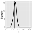
By working with a density estimate $\widehat{f}(z|\mathbf{x})$, instead of a point estimate of $z$, one can dramatically reduce systematic errors in downstream analysis, i.e., when estimating functions $g(z)$ of an unknown redshift $z$; see, for example, Mandelbaum et al. 2008; Wittman 2009; Sheldon et al. 2012. Although optimizing the function $g$ would be optimal for the problem of choice, often there is no clear $g$ ahead of time or there exist many different functions $g$ for the same application; for example, for the galaxy-galaxy lensing problem in Sec. 6, each of $\approx 500,000$ lenses has a different calibration function $g$. Hence, a common practice in astronomy is to build catalogs of photo-$z$ density estimates (for galaxies in a survey), which can then be used to address a range of different inference problems in astronomy and cosmology. Many of these estimates, however, include handpicked tuning parameters and, as we later show in Sec. 6 (Fig. 10), estimates that yield good results for a particular application or function of $z$ do not necessarily predict the redshift $z$ per se well. This brings up the question of how to properly construct and assess conditional density estimators, in general, and photo-$z$ estimators, in particular.

On the methodological side, photo-$z$ estimation presents challenges at the boundaries of current statistical research. There exist a wide range of sophisticated techniques for high-dimensional inference but few attempt to estimate full conditional densities or ratios of high-dimensional densities (see, e.g. Izbicki et al. 2014; Izbicki and Lee 2015 and references within). Even less is known about how to estimate conditional densities under selection bias. Statistics and machine learning procedures typically assume that training and test data have similar distributions but the two distributions can be very different for sky surveys that mix spectroscopy and photometry, and e.g. remote sensing applications where different sensors may malfunction at different rates or collect data at different rates (see Moreno-Torres et al. 2012 for data set shift in classification).

In the astronomy literature, existing photo-$z$ algorithms roughly fall into two categories. In the first category, template fitting (e.g., Fernández-Soto et al. 1998) estimates $f(z|\mathbf{x})$ by directly comparing observed data with a suite of idealized photometric data sets for different types of galaxies at different redshifts. Our interest lies in the second category, empirical redshift estimation, in which one builds an estimator of $f(z|\mathbf{x})$ using a training set of galaxies with spectroscopically confirmed redshifts (see, e.g., Ball and Brunner 2010; Zheng and Zhang 2012; Kind and Brunner 2013). In photo-$z$ estimation, however, high-resolution spectroscopy is extremely time-consuming. For example, one would already need $\sim$2.5 years of dedicated telescope time to estimate the spectroscopic redshifts for the 500,000-galaxy photometric SDSS sample in our paper; the problem only gets worse with deeper and larger surveys. As a result, usually only the rarest and brightest galaxies are spectroscopically observed, and these galaxies have characteristics and measured covariates that do not necessarily match those of more numerous dimmer galaxies (see, e.g., Oyaizu et al. 2008; Ball and Brunner 2010).

The goal of this paper is to develop improved nonparametric methods for conditional density estimation that explicitly deal with photo-$z$ estimation and selection bias:

1. On the methods side, we present a general framework for supervised learning that accounts for differences in training and test data, and that unlike standard nonparametric regression and classification can handle highly asymmetric and multimodal distributions. We design appropriate loss functions for a multivariate setting with selection bias (Eqs. 5 and 9), and we show how to estimate these functions using labeled and unlabeled data. Our set-up provides a principled method for choosing tuning parameters, for selecting covariates, and for comparing and combining (Sec. 5.4) different conditional density estimators for optimal performance. The final density estimates lead to more accurate predictive intervals (see, for example, Fig. 10) for new observations. Estimating $f(z|{\mathbf{x}})$ is also a simple way of performing nonparametric quantile regression of many quantiles simultaneously (Koenker, 2005).

2. In the context of photo-$z$ prediction, we propose more accurate algorithms for estimating photo-$z$ probability distributions in a setting where primarily nearby and bright galaxies have known redshifts. Using SDSS as well as simulated data, we analyze and compare different methods for estimating conditional densities and so-called importance weights (which are used to correct for selection bias). We introduce two new conditional density estimators, Kernel nearest neighbors (Sec. 5.2) and Series (Sec. 5.3), that both have better performance than the photo-z prediction method by Cunha et al. (2009), which represents the state-of-the-art for empirical photo-$z$ estimators under selection bias. We also present different diagnostic tests for evaluating the goodness-of-fit of estimated densities (Appendix A).

The organization of the paper is as follows: Sec. 2 describes our data. In Sec. 3, we introduce the statistical problem and the idea of importance weights. Sec. 4 compares different schemes for estimating these weights. Then, in Sec. 5, we shift our focus to the problem of estimating conditional densities under selection bias, and the issue of proper model selection and assessment. Finally, in Sec. 6, we offer some new insights on the galaxy lensing-lensing example from Sheldon et al. (2012). We conclude our work with Sec. 7.

2 Data

There are two main types of astronomical data: spectroscopic data, where both the covariates ${\mathbf{x}}$ and the redshift $z$ (the label) can be measured with negligible error, and (ii) photometric data, where only the covariates ${\mathbf{x}}$ are known and there is no precise measurement of the redshift. In our study, we use photometric and spectroscopic data from the Sloan Digital Sky Survey (SDSS; York et al. 2000), as well as SDSS-based simulated data with known levels of selection bias.

2.1 SDSS Photometric Data

Since 1998, SDSS has collected data on over 200 million galaxies that are spread across one-quarter of the sky. The vast majority ($\gtrsim$99%) of these galaxies are only photometrically observed.

In photometry, different filters are sequentially placed into a telescope’s light path. Each filter only allows passage of photons in a particular wavelength band. SDSS measures photon fluxes, or equivalently magnitudes (the logarithm of fluxes), in five bands, denoted $u$, $g$, $r$, $i$, and $z$, in the wavelength range $3.5\times 10^{-7}$ meters to $9\times 10^{-7}$ meters (i.e., from UV light through the optical regime to infrared light). Magnitude estimates are algorithm-dependent, in that they depend on how one defines a boundary around a galaxy and how one sums the light within that boundary. SDSS catalogs include estimates from many different boundary-definition algorithms or magnitude systems; in this work, we follow Sheldon et al. (2012) and use model and cmodel magnitudes. We also work with colors, or differences of magnitudes in adjacent wavelength bands.

Our final SDSS photometric data set contains 10 covariates (four colors and the associated $r$-band magnitude from each algorithm) for 538,974 galaxies in an $\approx$72 square-degree sky patch. These galaxies are extracted from SDSS Data Release 8 (DR8; Aihara et al. 2011) and filtered according to Sheldon et al. (2012). Each covariate is normalized to have mean 0 and standard deviation 1.

2.2 SDSS Spectroscopic Data

Of the over 200 million galaxies in SDSS, some one million have been the subject of follow-up spectroscopic observations. In spectroscopy, a light-dispersing grating or prism is placed into a telescope’s light path. The photon changes its path with an angle that is proportional to its wavelength. Thanks to high-resolution mapping of the dispersed light, one can finely resolve narrow spectral features (or lines) that are smeared out in photometry. These lines, which are caused by transitions of electrons between atomic energy levels, occur at known wavelengths $\lambda$ but are observed at wavelengths $(1+z)\lambda$, where $z$ is the galaxy’s redshift. One can use the wavelength ratios of two or more observed lines to infer which transitions they represent; once that information is known, redshift estimation is trivial. The precision in the estimates is typically ${\Delta z}/z\sim 10^{-6}$, i.e., for spectroscopic redshifts, we can safely ignore the measurement error.

In this paper, we use the same data (i.e., colors and $r$-band magnitudes, collectively denoted ${\mathbf{x}}$, and redshifts $z$) as in Sheldon et al. (2012). This data set includes 435,875 galaxies; the vast majority are taken from SDSS DR8 but some fainter galaxies have been added so that the spectroscopic covariates cover the same space as the photometric covariates, albeit with a different distribution (E. Sheldon, private communication).

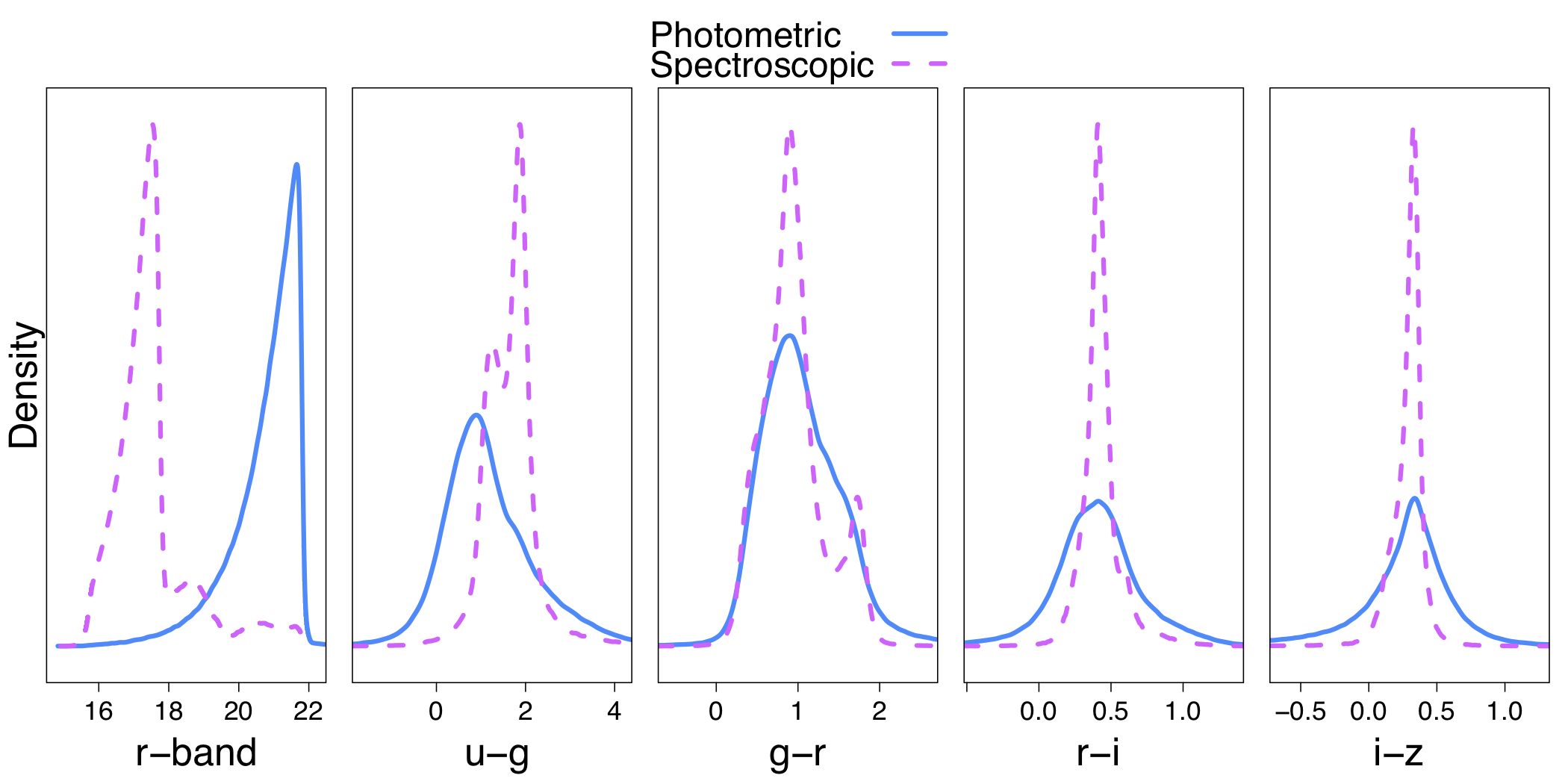
Fig. 2 shows the distributions of the spectroscopic and photometric samples. The left panel shows that there is a clear selection bias in the study where the galaxies in the spectroscopic sample tend to be brighter (i.e. they tend to have a lower $r$-band magnitude) than the galaxies in the photometric sample.

(a)

Figure 2: Distribution of $r$-band model magnitude and colors (i.e., differences of model magnitude values in adjacent photometric bins) for photometric versus spectroscopic SDSS data. Many galaxies in the spectroscopic sample are brighter (i.e. they have a lower $r$-band magnitude as indicated in the left panel) than the galaxies in the photometric sample.

2.3 Simulated Samples with Known Levels of Selection Bias

In addition to the SDSS data, we construct photometric samples with known levels of selection bias relative to the SDSS spectroscopic data. We use the following rejection sampling algorithm: Let $\mathbf{x}$ be a data point in the spectroscopic sample with $r$ model magnitude $x^{r}$ (scaled to be between $0$ and $1$). A large $r$ model magnitude corresponds to a faint galaxy. Let $S$ be a binary selection variable that decides whether a galaxy in the spectroscopic sample is included in the photometric sample ($S=1$) or not ($S=0$). We assume that the probability $P(S=1|\mathbf{x})$ depends on $\mathbf{x}$ through $x^{(r)}$ only; i.e., that $P(S=1|\mathbf{x})=P(S=1|x^{(r)})$. To create levels of selection bias realistic for different astronomical surveys, we resample the SDSS spectroscopic sample according to
Scheme 1: $P(S=1|x^{(r)})=f_{\mbox{B(1,1)}}(x^{(r)})\equiv 1$,
Scheme 2: $P(S=1|x^{(r)})=f_{\mbox{B(13,4)}}(x^{(r)})$,
Scheme 3: $P(S=1|x^{(r)})=f_{\mbox{B(18,4)}}(x^{(r)})$,
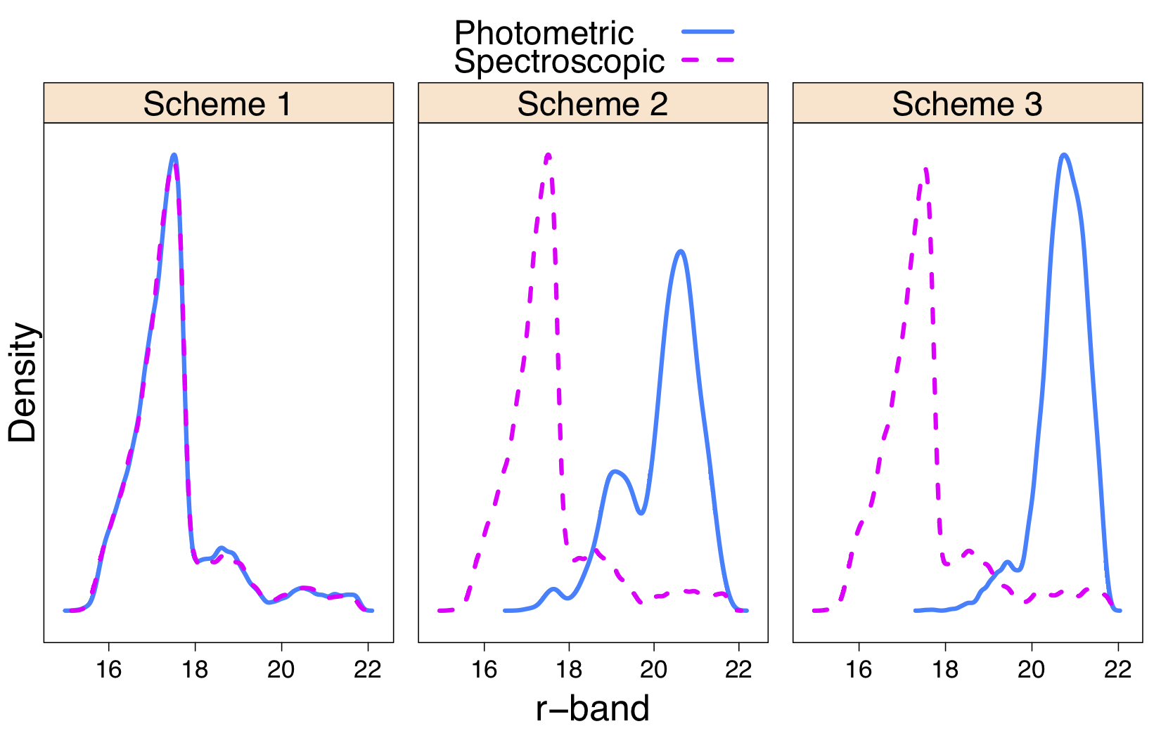
where $f_{\mbox{B(i,j)}}$ denotes the density of a beta random variable with parameters $(i,j)$. Fig. 3 shows the resulting $r$-band distributions. Scheme 1 involves no selection bias: the spectroscopic and photometric data have $r$-band magnitudes with the same distribution. At the other extreme is Scheme 3 with strong selection bias: most photometrically observed galaxies are significantly fainter (shifted toward large $r$-band magnitude) than the galaxies in the spectroscopic data set.

(a)

Figure 3: Distribution of the $r$-band model magnitudes for three different schemes of resampling the SDSS spectroscopic sample. The simulated data sets have (known) levels of selection bias realistic for different astronomical surveys.

3 Selection Bias, Covariate Shift and Importance Weights

A standard assumption in statistics and machine learning is that labeled and unlabeled data have similar distributions but, as Fig. 2 (left panel) shows, the two distributions can be very different for sky surveys that mix spectroscopy and photometry: Brighter galaxies (or galaxies with a lower $r$-band magnitude) are more likely to be selected for follow-up spectroscopic observation. This fact motivates the methods and algorithms presented in this paper. Below, we fix our notation and describe the main ideas behind importance weights as a way of correcting for sample selection bias.

3.1 Problem Statement and Notation

Our data are covariates $\mathbf{x}\in\mathbb{R}^{d}$ (photometric colors and magnitudes) and labels $z\in\mathbb{R}$ (the redshift). Without loss of generality, we rescale the original redshift values so that the response $z\in[0,1]$.

Suppose we have access to an i.i.d unlabeled sample $\mathbf{x}^{U}_{1},\ldots,\mathbf{x}^{U}_{n_{U}}$ with only photometric data, and an i.i.d. labeled sample $(\mathbf{x}^{L}_{1},z^{L}_{1}),\ldots,(\mathbf{x}^{L}_{n_{L}},z^{L}_{n_{L}})$ from a potentially different distribution, where the labels are from follow-up spectroscopic studies. Because the high cost of spectroscopy in sky surveys, in terms of telescopic resources, $n_{L}\ll n_{U}$ and the distributions of the labeled and unlabeled samples will not be the same. Our goal in this paper is to construct a photo-$z$ density estimator $\widehat{f}(z|\mathbf{x})$ that performs well on the unlabeled photometric data, which roughly dominate 99% of today’s galaxy observations.

To fix our notation, let ${\mathbb{P}}_{L}$ and ${\mathbb{P}}_{U}$ denote the distributions on the labeled and unlabeled samples, respectively; i.e., let $(\mathbf{x}^{L},z^{L})\sim{\mathbb{P}}_{L}$ and $(\mathbf{x}^{U},z^{U})\sim{\mathbb{P}}_{U}$, where $z^{U}$ are missing data labels. We say that there is a data set shift if ${\mathbb{P}}_{L}\neq{\mathbb{P}}_{U}$. To understand how this affects learning algorithms, one needs to make additional assumptions about the relationship between ${\mathbb{P}}_{L}$ and ${\mathbb{P}}_{U}$ (e.g., Quionero-Candela et al. 2009, Gretton et al. 2010, Moreno-Torres et al. 2012). For our application, we assume that the probability that a galaxy is labeled with a spectroscopic redshift is independent of the response variable $z$ if we condition on the covariates $\mathbf{x}$ (Lima et al. 2008; Sheldon et al. 2012); i.e.,

$${\mathbb{P}}(S=1|\mathbf{x},z)={\mathbb{P}}(S=1|\mathbf{x})\ ,$$ (1)

where the random variable $S$ equals $1$ if a datum is labeled and $0$ otherwise. This type of sample selection bias where Eq. 1 holds is sometimes referred to as missing at random (MAR; Rubin 1976, Moreno-Torres et al. 2012) bias. MAR bias implies covariate shift, defined as

$$f_{L}(\mathbf{x})\neq f_{U}(\mathbf{x}),\ \ f_{L}(z|\mathbf{x})=f_{U}(z|\mathbf{x}).$$ (2)

Under certain conditions on the support of $f_{L}(\mathbf{x})$ and $f_{U}(\mathbf{x})$, covariate shift also implies MAR bias (Moreno-Torres et al. 2012). Below we use the terms interchangeably to refer to the assumption in Eq. 1.

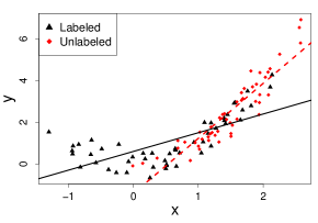
At first glance, it may seem that MAR bias would not pose a problem for density estimation: Because $f(z|\mathbf{x})$ is the same for both labeled and unlabeled samples (Eq. 2), one might conclude that a good estimator of $f(z|\mathbf{x})$ based on labeled data would also have good performance for unlabeled data. This is in general not true. Often $f(z|\mathbf{x})$ is well estimated only in regions where there is plenty of labeled data and these regions may not coincide with regions where there is plenty of unlabeled (target) data; see Figure 4 for a toy example of an equivalent regression problem with covariate shift. From a statistical perspective, this problem arises because the loss function used for estimating $f(z|\mathbf{x})$ (or analogously $\mathbb{E}[z|\mathbf{x}]$ in regression) depends on the marginal distribution of $\mathbf{x}$. Hence, an estimator that performs well with respect to $f_{L}(\mathbf{x})$ may not perform well with respect to $f_{U}(\mathbf{x})$.

Figure 4: Toy example for covariate shift in linear regression: The solid line is reasonable for predicting new data from the labeled sample, but it is far from optimal for the unlabeled sample.

One solution to this mismatch problem is to reweight the labeled data so that their distribution ${\mathbb{P}}_{L}$ – after a reweighing with the so-called importance weights $\beta(\mathbf{x}):=f_{U}(\mathbf{x})/f_{L}(\mathbf{x})$ – matches the distribution ${\mathbb{P}}_{U}$ of the unlabeled data. We can then compute expectations with respect to the target distribution ${\mathbb{P}}_{U}$ using the distribution ${\mathbb{P}}_{L}$ of the labeled training data. In particular, if $l(\widehat{f},f)$ is the loss function for the estimated conditional density $\widehat{f}$, we use that

$$\mathbb{E}_{({\mathbf{X}},Z)\sim{\mathbb{P}}_{U}}\left[l(\widehat{f}(Z|{\mathbf{X}}),f(Z|{\mathbf{X}}))\right]=\mathbb{E}_{({\mathbf{X}},Z)\sim{\mathbb{P}}_{L}}\left[l(\widehat{f}(Z|{\mathbf{X}}),f(Z|{\mathbf{X}}))\beta({\mathbf{X}})\right].$$ (3)

The last expression of Eq. 3 involves unknown weights $\beta({\mathbf{x}})$. Open questions are:

1. how to best estimate the importance weights $\beta(\mathbf{x}):=f_{U}(\mathbf{x})/f_{L}(\mathbf{x})$, where ${\mathbf{x}}$ is our multivariate data, and

2. how to design an estimator of the full conditional density $f(z|\mathbf{x})$ that performs well on the target data; i.e., that has a small risk according to Eq. 3.

In this work, we propose a greedy two-step approach to conditional density estimation under selection bias where one first selects the best model for estimating $\beta(\mathbf{x})$ (see Sec. 4), and then uses these estimates to search for the best model for estimating $f(z|\mathbf{x})$ under covariate shift (see Sec. 5). Note that a necessary condition for computing importance weights is that ${\mathbb{P}}_{L}$ dominates ${\mathbb{P}}_{U}$, i.e., ${\mathbb{P}}_{L}(\mathbf{x})\gg{\mathbb{P}}_{U}(\mathbf{x})$; hence, for this study, we have selected photometric data whose covariates lie within the domain of the spectroscopic covariates (see Sec. 2.1).

4 Estimating Importance Weights

A naive method for computing $\beta(\mathbf{x})$ is to separately estimate $f_{U}$ and $f_{L}$ and to then take their ratio, but this approach can enhance errors in the individual density estimates, particularly in regions where $f_{L}$ is nearly zero (Sugiyama et al., 2008). There are also several other approaches for estimating density ratios (see Appendix B).

The goal in this section is to find out how these estimators perform in practice on our data. To assess the estimators, we use the weighted loss function by Izbicki et al. (2014) defined as

$$L(\widehat{\beta},\beta): =\int\left(\widehat{\beta}(\mathbf{x})-\beta(\mathbf{x})\right)^{2}dP_{L}(\mathbf{x})$$

$$=\int\widehat{\beta}^{2}(\mathbf{x})dP_{L}(\mathbf{x})-2\int\widehat{\beta}(\mathbf{x})dP_{U}(\mathbf{x})+K,$$ (4)

where $K$ is a constant that does not depend on $\widehat{\beta}(\mathbf{x})$. (Appendix B gives some intuition behind the choice of this loss function.) We divide our data into three parts: a training set used to fit the model, a validation set for model selection and tuning of parameters, and a test set for assessing the final model (Hastie et al., 2009, p. 222). For model selection and model assessment, we estimate $L(\widehat{\beta},\beta)$ according to Izbicki et al. (2014):

$$\widehat{L}(\widehat{\beta},\beta)=\frac{1}{\widetilde{n}_{L}}\sum_{k=1}^{\widetilde{n}_{L}}\widehat{\beta}^{2}\left(\widetilde{\mathbf{x}}_{k}^{L}\right)-2\frac{1}{\widetilde{n}_{U}}\sum_{k=1}^{\widetilde{n}_{U}}\widehat{\beta}\left(\widetilde{\mathbf{x}}_{k}^{U}\right),$$ (5)

where $\widetilde{\mathbf{x}}^{L}_{1},\ldots,\widetilde{\mathbf{x}}^{L}_{\widetilde{n}_{L}}$ represent the labeled (validation or test) data, and $\widetilde{\mathbf{x}}^{U}_{1},\ldots,\widetilde{\mathbf{x}}^{U}_{\widetilde{n}_{U}}$ represent the unlabeled (validation or test) data.

Experiments. We use this loss function to compare six different estimators of $\beta$:

• $\beta$-NN, the nearest neighbor estimator from Lima et al. (2008) (Eq. 20 in the Appendix B), but with the number of nearest neighbors $M$ chosen so as to minimize our estimated loss (Eq. 5) on the validation data (as in Kremer et al. 2015);

• $\beta$-NN1, the nearest neighbor approach with $M=1$ (Loog, 2012);

• $\beta$-KLIEP and $\beta$-uLSIF, importance weight estimators suggested by Sugiyama et al. (2008) and Kanamori et al. (2009), respectively, and implemented with the authors’ MATLAB code;

• $\beta$-KuLSIF, a kernelized version of $\beta$-uLSIF (Kanamori et al., 2012); and

• $\beta$-Series, the density ratio estimator from Izbicki et al. (2014).

Following Lima et al. (2008), our covariates are the four colors and the $r$-band magnitude in the model magnitude system.

We study the estimators under the simulated selection bias settings from Section 2.1 (Schemes 1-3), using labeled and unlabeled samples that are each of size 10,000. (For each sample, we randomly choose 2,800 galaxies for training, 1,200 for validation and 6,000 for testing.) We also apply the estimators to the SDSS data. These data have a large covariate shift (Fig. 2). where $\widehat{\beta}(\mathbf{x})=0$ for $\approx$80% of the labeled examples, i.e., the majority of the spectroscopic sample lie in regions of covariate space where there are no unlabeled data. Having more labeled data may seem harmless but it turns out that if one includes these labeled examples in the training sample, the effective sample size (defined in Shimodaira 2000 and Gretton et al. 2010) will be very small, ultimately resulting in poor conditional density estimates (see Sec. 5.5 and Fig. 8). Essentially, many galaxies have zero weight (i.e. no contribution) in the conditional density estimation. To mitigate this problem, we use a similar data cleaning step as in Lima et al. (2008): First, we construct a $\beta$-NN estimator using a preliminary sample of 10,000 spectroscopic and 10,000 photometric (randomly selected) galaxies. Using this estimate, we then create a new spectroscopic sample of size 15,000 which consists of galaxies with weight estimates $\widehat{\beta}(\mathbf{x})\neq 0$. The SDSS results in this paper are based on the new spectroscopic sample together with 15,000 randomly selected photometric observations; Fig. 5 shows the distributions of the two samples after the preprocessing step. In all experiments on SDSS data, we use $3,\!500$ galaxies from each sample (labeled and unlabeled) for training, $1,\!500$ for validation, and the remainder for testing.

(a)

Figure 5: Distribution of the $r$-band model magnitude and the four colors from model magnitude for the SDSS photometric and spectroscopic samples after we remove and replace labeled examples for which the initial estimates of the importance weights are zero; compare with Fig. 2. By restricting the labeled data to the regions of interest (i.e. to the regions where there are unlabeled data) we increase the effective sample size.

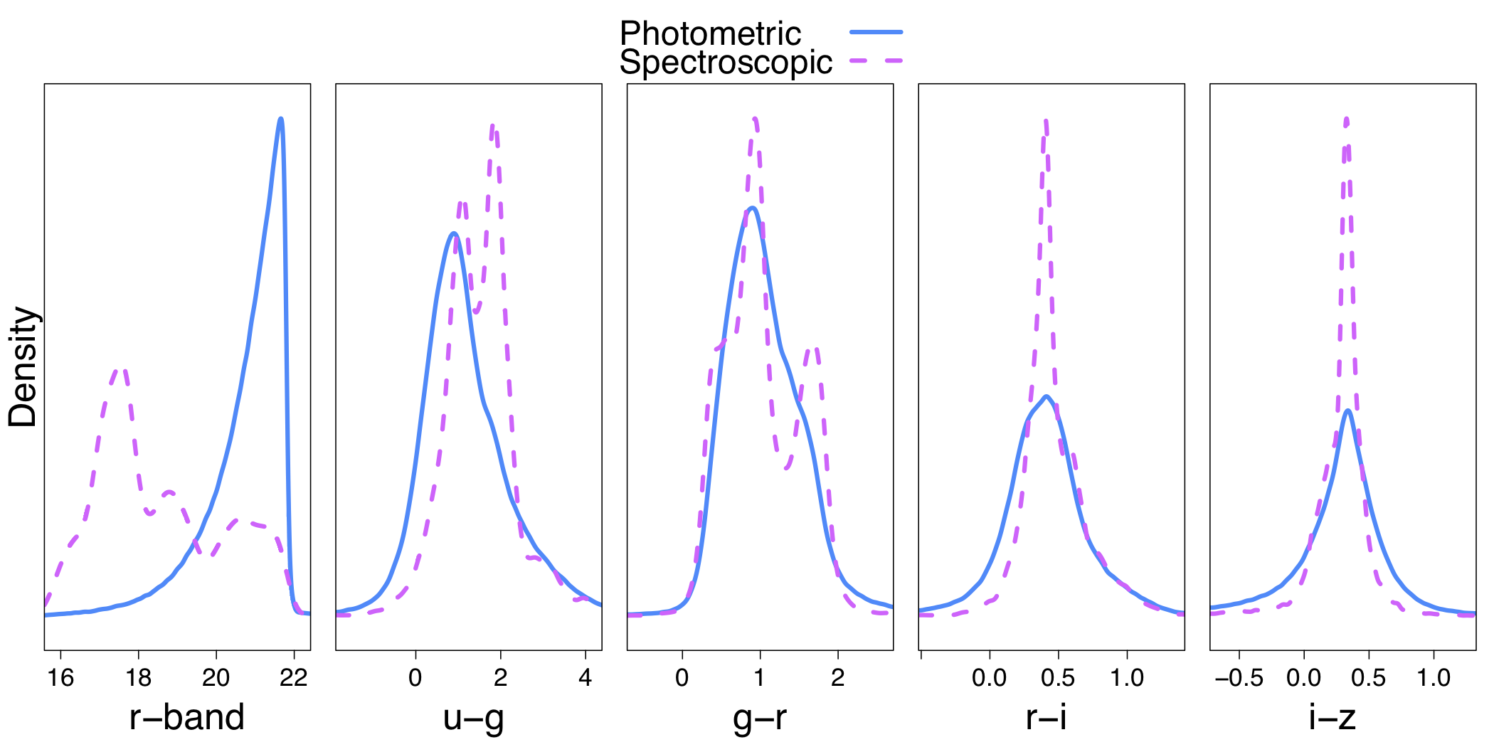
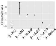
Fig. 6 compares the different estimators of $\beta$. The nearest-neighbor method is rarely mentioned in the literature on data set shift, but in our experiments we find that $\beta$-NN, where $M$ is chosen by data splitting, consistently performs the same or better than other competing (and more complicated) methods; $\beta$-Series is a close second. This is in agreement with recent independent work by Kremer et al. (2015). We also note that by minimizing Eq. 5, we select $M=8$ neighbors for the SDSS dataset, a value similar to the value $M=5$ chosen in an ad hoc manner by Cunha et al. (2009). Henceforth, we will use the $\beta$-NN method (defined in Appendix B, Eq. 20) to estimate importance weights.

(a) Scheme 1

(b) Scheme 2

(c) Scheme 3

(d) SDSS

Figure 6: The estimated loss $\widehat{L}(\widehat{\beta},\beta)$ of different estimators of $\beta(\mathbf{x})$ for Schemes 1-3 with, respectively, (a) no, (b) moderate, and (c) large covariate shift. Panel (d) shows $\widehat{L}(\widehat{\beta},\beta)$ for observed SDSS data. The bars in each panel correspond to the mean estimated loss $\pm 1$ standard error. These results indicate that $\beta$-NN consistently performs the same or better than other competing methods; $\beta$-Series is a close second.

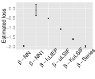
Variable Selection. One can further improve on these results by variable selection on the full set of 10 covariates. Table 1 lists the selected covariates in a forward stepwise model search with $\beta$-NN. For Scheme 1, where there is no selection bias (and where $\beta({\mathbf{x}})$, as a result, does not depend on ${\mathbf{x}}$), the final model includes only one covariate. In Schemes 2 and 3, the importance weights depend on the model $r$-band magnitude, and the selected model always includes this covariate. For the SDSS data, we achieve a loss of $-2.41\pm 0.08$ with variable selection, which is significantly smaller than the value $-2.16\pm 0.05$ when including all 10 covariates, and the value $-1.97\pm 0.04$ (see $\beta$-NN in Fig. 6d) when using the five covariates from the model magnitude system only as in Sheldon et al. (2012).

Table 1: Selected covariates for estimating importance weights with the $\beta$-NN estimator.

Data set	model					cmodel
	$r$	$u-g$	$g-r$	$r-i$	$i-z$	$r$	$u-g$	$g-r$	$r-i$	$i-z$
Scheme 1			X
Scheme 2	X					X			X
Scheme 3	X	X
SDSS	X	X				X	X	X

5 Conditional Density Estimation under Covariate Shift

Conditional density estimators are typically designed to minimize the loss

$$\iint\left(\widehat{f}(z|\mathbf{x})-f(z|\mathbf{x})\right)^{2}dP_{L}(\mathbf{x})dz$$ (6)

under the implicit assumption that ${\mathbb{P}}_{L}={\mathbb{P}}_{U}$. One can easily estimate this loss (up to a constant) using the labeled data:

$$\frac{1}{\widetilde{n}_{L}}\sum_{k=1}^{\widetilde{n}_{L}}\int\widehat{f}^{2}\left(z|\widetilde{\mathbf{x}}_{k}^{L}\right)dz-2\frac{1}{\widetilde{n}_{L}}\sum_{k=1}^{\widetilde{n}_{L}}\widehat{f}\left(\widetilde{z}^{L}_{k}|\widetilde{\mathbf{x}}^{L}_{k}\right).$$ (7)

However, our goal is really to minimize

$$L(\widehat{f},f):=\iint\left(\widehat{f}(z|\mathbf{x})-f(z|\mathbf{x})\right)^{2}dP_{U}(\mathbf{x})dz\,,$$ (8)

where ${\mathbb{P}}_{U}$ is the distribution of the unlabeled target data. The two losses can be very different if ${\mathbb{P}}_{L}\neq{\mathbb{P}}_{U}$. Hence, a density estimator that performs well on the labeled data may not be a good estimator for the data of interest; Fig 4 shows a similar problem in linear regression.

The challenge is to estimate Eq. 8 without knowing $z$ at the unlabeled data points. Under the covariate shift assumption $f_{U}(z|\mathbf{x})=f_{L}(z|\mathbf{x})$, one can use importance sampling. Up to a constant, Eq. 8 becomes

$$L(\widehat{f},f) =\iint\widehat{f}^{2}(z|\mathbf{x})dP_{U}(\mathbf{x})dz-2\iint\widehat{f}(z|\mathbf{x})f(z|\mathbf{x})dP_{U}(\mathbf{x})dz$$

$$=\iint\widehat{f}^{2}(z|\mathbf{x})dP_{U}(\mathbf{x})dz-2\iint\widehat{f}(z|\mathbf{x})\beta(\mathbf{x})dP_{L}(z,\mathbf{x})\,,$$

where we for the second equality use that $f_{U}(z|\mathbf{x})dP_{U}(\mathbf{x})dz=f_{L}(z|\mathbf{x})\beta(x)dP_{L}(\mathbf{x})dz=\beta(x)dP_{L}(z,\mathbf{x})$. Hence, when ${\mathbb{P}}_{L}\neq{\mathbb{P}}_{U}$, we replace the standard empirical loss in Eq. 7 by

$$\widehat{L}(\widehat{f},f)=\frac{1}{\widetilde{n}_{U}}\sum_{k=1}^{\widetilde{n}_{U}}\int\widehat{f}^{2}\left(z|\widetilde{\mathbf{x}}_{k}^{U}\right)dz-2\frac{1}{\widetilde{n}_{L}}\sum_{k=1}^{\widetilde{n}_{L}}\widehat{f}\left(\widetilde{z}^{L}_{k}|\widetilde{\mathbf{x}}^{L}_{k}\right)\widehat{\beta}\left(\widetilde{\mathbf{x}}^{L}_{k}\right).$$ (9)

We can compute this loss using (labeled and unlabeled) validation data and $\widehat{\beta}\left(\widetilde{\mathbf{x}}^{L}_{k}\right)$, which are estimates of the importance weights at the labeled data points.

In what follows (Secs. 5.1-5.4), we present four conditional density estimators specifically designed for multivariate data and a covariate shift (CS) setting: NN_CS, ker-NN_CS, $Series_{CS}$, and Comb_CS. The NN_CS nearest-neighbor histogram estimator first appeared in Cunha et al. (2009); the other estimators represent novel approaches. For model selection and tuning of parameters, we minimize Eq. 9 with importance weights $\beta$ estimated via Eqs. 20 and 5. The same loss is also used for model assessment of the SDSS data. For model assessment of the simulated data (where we know the true labels $\widetilde{z}^{U}$), we compute the more accurate error estimate

$$\widehat{L}(\widehat{f},f)=\frac{1}{\widetilde{n}_{U}}\sum_{k=1}^{\widetilde{n}_{U}}\int\widehat{f}^{2}\left(z|\widetilde{\mathbf{x}}_{k}^{U}\right)dz-2\frac{1}{\widetilde{n}_{U}}\sum_{k=1}^{\widetilde{n}_{U}}\widehat{f}\left(\widetilde{z}^{U}_{k}|\widetilde{\mathbf{x}}^{U}_{k}\right),$$ (10)

which does not involve importance weights $\beta$.

Remark 1 (Choice of Loss Function).

One can replace the averaged $L^{2}$-loss in Eq. 8 with other measures of discrepancy, but many of the distance measures common in discrimination analysis (e.g. $F$-divergences and differences in log-densities) are profoundly sensitive to the tails of the distribution and not suitable for density estimation; see e.g. Hall (1987) and Wasserman (2006).

5.1 Nearest-Neighbor Histogram (NN_CS)

In Cunha et al. (2009), the authors use a weighted nearest-neighbor histogram to estimate the photo-$z$ distribution of a galaxy with photometric covariates ${\mathbf{x}}$. Let $\mathcal{N}_{N}(\mathbf{x})$ denote the $N$ nearest neighbors of $\mathbf{x}$ among the labeled data. Divide $[0,1]$, the range of $z$, into $B$ equal-sized bins, and let $b(z)$ denote the bin that includes $z$ for $z\in[0,1]$. Then, the weighted histogram estimator is

$$\widehat{f}(z|\mathbf{x})\propto\sum_{k\in\mathcal{N}_{N}(\mathbf{x})}\widehat{\beta}\left(\mathbf{x}^{L}_{k}\right){\mathbb{I}}\left(z^{L}_{k}\in b(z)\right)\,,$$ (11)

where the importance weights $\widehat{\beta}(\mathbf{x}^{L}_{k})$ reflect how representative each labeled galaxy $k\in\mathcal{N}_{N}(\mathbf{x})$ is of the target distribution. Cunha et al. choose the tuning parameters in their model by hand. Here we use Eq. 9 to find the optimal values of $N$ and $B$ for the conditional density estimator in Eq. 11, and we use Eq. 5 to select the best value of $M$ in Eq. 20 for computing the weights $\widehat{\beta}(\mathbf{x})$.

5.2 Kernel Nearest-Neighbor Estimator (ker-NN_CS)

A simple way of improving upon $NN_{CS}$ is to replace the indicator function in Eq. 11 with a kernel smoother:

$$\widehat{f}(z|\mathbf{x})\propto\sum_{k\in\mathcal{N}_{N}(\mathbf{x})}\widehat{\beta}\left(\mathbf{x}^{L}_{k}\right)K_{\epsilon}\left(z-z^{L}_{k}\right)\,,$$ (12)

where, e.g., $K_{\epsilon}(z\!-\!z_{k})\!=\!e^{-\left(z\!-\!z_{k}\right)^{2}\!/\!4\epsilon}$. As before, we choose the tuning parameters (here, $N$ and $\epsilon$ in Eq. 12, and $M$ in Eq. 20) that minimize the estimated losses in Eqs. 9 and 5. This estimator leads to much more accurate density estimates than its histogram equivalent when we have limited amounts of labeled data (and hence small values of $N$).

5.3 Spectral Series CDE under Covariate Shift (Series_CS)

Suppose that the covariates $\mathbf{x}$ lie in a lower-dimensional subspace $\mathcal{X}$ of $\mathbb{R}^{d}$, where the number of covariates $d$ may be large. Izbicki and Lee (2015) propose a spectral series estimator that expands the conditional density $f(z|\mathbf{x})$ in a basis $\Psi_{i,j}(z,\mathbf{x})=\phi_{i}(z)\psi_{j}(\mathbf{x})$ adapted to the intrinsic (lower-dimensional) geometry of a reference distribution ${\mathbb{P}}$ on $\mathcal{X}$. Here we generalize the series approach to a setting with covariate shift. We choose ${\mathbb{P}}_{L}$ as the reference distribution and tune the estimator so as to minimize the loss with respect to ${\mathbb{P}}_{U}$.

More specifically: We assume the functions $\phi_{i}$ to be standard (one-dimensional) Fourier basis functions, whereas the functions $\psi_{j}$ are the eigenfunctions of the operator $\textbf{K}:L^{2}(\mathcal{X},{\mathbb{P}}_{L})\longrightarrow L^{2}(\mathcal{X},{\mathbb{P}}_{L})$,

$$\textbf{K}(h)(\mathbf{x})=\int_{\mathcal{X}}K(\mathbf{x},\mathbf{y})h(\mathbf{y})dP_{L}(\mathbf{y}),$$ (13)

where $K(\mathbf{x},\mathbf{y})$ is a bounded, symmetric, and positive definite kernel. By construction (Minh et al., 2006; Izbicki and Lee, 2015),

$$\int_{\mathcal{X}}\psi_{i}(\mathbf{x})\psi_{j}(\mathbf{x})dP_{L}(\mathbf{x})=\delta_{i,j}\overset{\mbox{\tiny{def}}}{=}{\mathbb{I}}(i=j).$$ (14)

As a result, the coefficients in the series expansion are simply expectations over the eigenfunctions:

$$\alpha_{i,j} =\iint f(z|\mathbf{x})\Psi_{i,j}(z,\mathbf{x})dP_{L}(\mathbf{x})dz={\mathbb{E}}_{({\mathbf{X}},Z)\sim{\mathbb{P}}_{L}}[\Psi_{i,j}(Z,\mathbf{X})]\,.$$ (15)

In practice, we need to estimate both the functions $\psi_{j}$ and the coefficients $\alpha_{i,j}$ from data: Using the labeled training examples, we compute the first $J$ eigenvectors $\widetilde{\psi}_{1},\ldots,\widetilde{\psi}_{J}$ of the Gram matrix

$$\left[K\left(\mathbf{x}^{L}_{i},\mathbf{x}^{L}_{j}\right)\right]_{i,j=1}^{n},$$

where $K(\mathbf{x},\mathbf{y})=\exp{\left(-d^{2}(\mathbf{x},\mathbf{y})/4\epsilon\right)}$ is the Gaussian kernel. We then extend these vectors to out-of-sample points via the Nyström extension

$$\widehat{\psi}_{j}(\mathbf{x})=\frac{\sqrt{n_{L}}}{\widehat{l}_{j}}\sum_{k=1}^{n_{L}}\widetilde{\psi}_{j}\left(\mathbf{x}^{L}_{k}\right)K\left(\mathbf{x},\mathbf{x}^{L}_{k}\right),$$ (16)

where $\widehat{l}_{j}$ is the eigenvalue associated to the eigenvector $\left(\widetilde{\psi}_{j}(\mathbf{x}^{L}_{1}),\ldots,\widetilde{\psi}_{j}(\mathbf{x}^{L}_{n_{L}})\right)$. Next we estimate the expansion coefficients in Eq. 15 according to

$$\widehat{\alpha}_{i,j}=\frac{1}{n_{L}}\sum_{k=1}^{n_{L}}\widehat{\Psi}_{i,j}(z_{k}^{L},\mathbf{x}_{k}^{L})\,,$$

i.e., we average the empirical basis functions $\widehat{\Psi}_{i,j}(z_{k},\mathbf{x}_{k})=\phi_{i}(z_{k})\widehat{\psi}_{j}(\mathbf{x}_{k})$ over the labeled data. We define the new series estimator Series_CS by

$$\widehat{f}(z|\mathbf{x})=\sum_{i=1}^{I}\sum_{j=1}^{J}\widehat{\alpha}_{i,j}\widehat{\Psi}_{i,j}(z,\mathbf{x})\,,$$ (17)

where the parameters $I$, $J$, and $\epsilon$ are chosen so as to minimize the loss in Eq. (9) relative to the unlabeled data $P_{U}$.

5.4 Combined Estimator (Comb_CS)

Finally, we present a procedure for combining, or stacking, multiple estimators in a principled way. Suppose that $\widehat{f}_{1}(z|\mathbf{x}),\ldots,\widehat{f}_{p}(z|\mathbf{x})$ are different estimators of $f(z|\mathbf{x})$; these estimators could, for example, be any of the cross-validated estimators described in Secs. 5.1-5.3. Now ask the question: Can we average these models so as to reduce the prediction performance of individual estimators? If we restrict ourselves to weighted averages, then the answer is to compute

$$\widehat{f}^{{\boldsymbol{\alpha}}}(z|\mathbf{x})=\sum_{k=1}^{p}\alpha_{k}\widehat{f}_{k}(z|\mathbf{x}),$$

where the weights minimize the empirical loss $\widehat{L}(\widehat{f}^{{\boldsymbol{\alpha}}},f)$ in Eq. 9 under the constraints $\alpha_{i}\geq 0$ and $\sum_{i=1}^{p}\alpha_{i}=1$. The weights ${\boldsymbol{\alpha}}=\left[\alpha_{i}\right]_{i=1}^{p}$ can then be found by solving a standard quadratic programming problem:

$$\underset{{\boldsymbol{\alpha}}:\alpha_{i}\geq 0,\sum_{i=1}^{p}\alpha_{i}=1}{\arg\min}{\boldsymbol{\alpha}}^{\prime}\mathbb{B}{\boldsymbol{\alpha}}-2{\boldsymbol{\alpha}}^{\prime}b,$$ (18)

where $\mathbb{B}$ is the $p\times p$ matrix $\left[\frac{1}{\widetilde{n}_{U}}\sum_{k=1}^{\widetilde{n}_{U}}\int\widehat{f}_{i}(z|\widetilde{\mathbf{x}}_{k}^{U})\widehat{f}_{j}(z|\widetilde{\mathbf{x}}_{k}^{U})dz\right]_{i,j=1}^{p}$ and $b$ is the vector $\left[\frac{1}{\widetilde{n}_{L}}\sum_{k=1}^{\widetilde{n}_{L}}\widehat{f}_{i}(\widetilde{z}^{L}_{k}|\widetilde{\mathbf{x}}^{L}_{k})\widehat{\beta}(\widetilde{\mathbf{x}}^{L}_{k})\right]_{i=1}^{p}.$

In this work, Comb_CS denotes the estimator that combines the two estimators ker-NN_CS and Series_CS, although this procedure of combining models applies more generally to other conditional density estimators.

5.5 Experiments

Using the simulated and observed data (Sec. 2), we will now compare the performance of seven different estimators of $f(z|{\mathbf{x}})$. (As before, our covariates are the four colors and the $r$-band magnitude in the model magnitude system. We split our data into training, validation, and test sets as in Sec. 4.) The first three estimators do not account for selection bias. They are

• NN: the nearest neighbor estimator from Sec. 5.1 with $\widehat{\beta}(\mathbf{x})\equiv 1$ for all $\mathbf{x}$;

• ker-NN: the kernel nearest neighbor estimator from Sec. 5.2 with $\widehat{\beta}(\mathbf{x})\equiv 1$ for all $\mathbf{x}$; and

• Series: the spectral series estimator from Izbicki and Lee (2015).

The tuning parameters of these three estimators minimize the empirical loss in Eq. 7 on the (labeled) validation data. The second three estimators correct for covariate shift by importance weights. They are

• NN_CS: the nearest neighbor estimator from Sec. 5.1;

• ker-NN_CS: the kernel nearest neighbor estimator from Sec. 5.2; and

• Series_CS: the spectral series estimator from Sec. 5.3.

Finally, we have

• Comb_CS: an estimator that combines ker-NN_CS and Series_CS according to Sec. 5.4.

We choose the tuning parameters of these last four estimators so as to minimize the reweighted empirical loss $\widehat{L}(\widehat{f},f)$ in Eq. 9 on (labeled and unlabeled) validation data. By bootstrap, we estimate the standard error of $\widehat{L}(\widehat{f},f)$ according to $\sqrt{{\mathbb{V}}\left[\widehat{L}(\widehat{f},f)\right]}\approx\sqrt{B^{-1}\sum_{b=1}^{B}\left(\widehat{L}_{b}(\widehat{f},f)-\overline{\widehat{L}(\widehat{f},f)}\right)^{2}},$ where $B=500$ is the number of bootstrap samples of the test set, $\widehat{L}_{b}(\widehat{f},f)$ is the estimated loss for the $b$th bootstrap sample, and $\overline{\widehat{L}(\widehat{f},f)}$ is the mean of $\{\widehat{L}_{b}(\widehat{f},f)\}_{b=1}^{B}$. Note that each bootstrap sample consists of a sample with replacement from the labeled set and a sample with replacement from the unlabeled set.

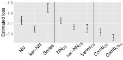
Fig. 7 shows the empirical loss (Eq. 10) on the test set for the simulated samples with known covariate shifts. Fig. 8a shows the estimated loss (Eq. 9) for 15,000 SDSS samples with no preprocessing, and Fig. 8b shows the loss after removing and replacing training examples with estimated weights $\widehat{\beta}({\mathbf{x}})\!=\!0$ so as to increase the effective sample size; note that the scales in these two plots differ.

(a) Scheme 1

(b) Scheme 2

(c) Scheme 3

Figure 7: Estimated loss of different density estimators for Schemes 1-3 with, respectively, (a) no, (b) moderate, and (c) large covariate shift. Bars correspond to mean plus and minus standard error. ker-NN is robust to selection bias and has a much smaller loss than previously proposed NN estimators (NN and NN_CS) even without importance weights; see text for discussion.

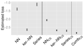
Variable Selection. As in Sec. 4, one can further improve these results by choosing a subset of the ten covariates from the model and cmodel magnitude systems. Table 2 lists the covariates from a forward stepwise model search with the combined estimator, initialized by an estimate of the marginal distribution $f(z)$. For the SDSS data, the loss of the combined estimator with variable selection (Comb${}_{{CS}_{VS}}$ in Fig. 8b) is $-2.51\pm 0.09$, which is smaller than $-2.36\pm 0.10$, the loss achieved by the combined estimator (Comb_CS) based on a fixed set of five model covariates.

(a) Original Sample

(b) After removing $\widehat{\beta}(\mathbf{x})=0$

Figure 8: Estimated loss of conditional density estimators for SDSS data (a) in the original sample with no preprocessing, and (b) after removing and replacing labeled examples for which the initial weight estimates $\widehat{\beta}({\mathbf{x}})=0$. Note that the scales in the two plots differ.

Table 2: Selected covariates for conditional density estimation with Comb${}_{{CS}_{VS}}$

Data set	model					cmodel
	$r$	$u-g$	$g-r$	$r-i$	$i-z$	$r$	$u-g$	$g-r$	$r-i$	$i-z$
Scheme 1	X	X	X	X	X			X	X	X
Scheme 2	X		X	X		X
Scheme 3	X		X	X		X
SDSS	X		X	X		X

Summary. Our main conclusions are as follows.

1. A necessary condition for importance weighting is that $\mathbb{P}_{L}$ dominates $\mathbb{P}_{U}$. Our results (Fig. 8) show that one should also restrict the labeled data to regions where there is unlabeled data; a simple procedure is to search for labeled examples with $\widehat{\beta}({\mathbf{x}})=0$ and replace these data with new labeled examples with $\widehat{\beta}({\mathbf{x}})\neq 0$.

2. Our kernel-based estimators ker-NN and ker-NN_CS consistently perform better than their histogram counterparts NN and NN_CS introduced by Cunha et al. (2009).

3. Interestingly, ker-NN is robust to selection bias even without explicitly incorporating importance weights into the estimator. Here is an intuitive explanation: If the neighborhood $N(\mathbf{x}_{0})$ around $\mathbf{x}_{0}$ is sufficiently small, then the covariate shift assumption (Eq. 2) implies that $f_{L}[z|\mathbf{x}\in N(\mathbf{x}_{0})]\approx f_{U}[z|\mathbf{x}\in N(\mathbf{x}_{0})]$. As a result, ker-NN returns good density estimates even without correcting for selection bias. NN is less robust than ker-NN because smoothing via binning requires larger neighborhoods (over which the above approximation may not hold) than smoothing via kernels. For example, in Scheme 3, $N$ = 35 for NN, versus 8 for ker-NN.

4. Series is sensitive to selection bias, but its covariate shift-corrected analogue Series_CS, which we introduce in this work, is one of the best estimators for conditional density estimation. When there is no selection bias (Fig. 7a), spectral series (Series and Series_CS) perform significantly better than nearest neighbors methods (ker-NN and ker-NN_CS); this result is consistent with earlier work by Izbicki and Lee (2015) on Series. In settings with covariate shift (Fig. 7b-c and Fig. 8b), Series_CS and ker-NN_CS are comparable. We conjecture that Series_CS may lose some of its competitive edge when ${\mathbb{P}}_{L}\neq{\mathbb{P}}_{U}$ because we compute the eigenvectors in the series using only labeled data, and then extrapolate to regions of the unlabeled data via the Nyström extension (Eq. 16).

5. However, by combining ker-NN_CS and Series_CS as in Sec. 5.4 we automatically get “the best of both worlds” under a variety of different settings. (The combined estimator Comb_CS assigns weights $\alpha\!=\!0.96$, 0.50, and 0.43 to Series_CS in Schemes 1-3, and $\alpha\!=\!0.53$ for the SDSS data.)

6. Finally, we can further improve our predictions by variable selection according to Secs. 4 and 5.5 when estimating $\beta({\mathbf{x}})$ and $f(z|{\mathbf{x}})$, respectively. Selection bias leads to smaller models with fewer variables (see Table 2), which is consistent with covariate shift decreasing the effective sample size (Shimodaira, 2000; Gretton et al., 2010), and thereby, increasing the variance of the estimators.

Algorithm 1 summarizes the combined model with variable selection (Comb${}_{{CS}_{VS}}$). This model includes two main steps, where we (i) first estimate the importance weights via $\beta$-NN with variable selection (lines 1-9), and (ii) then estimate the conditional density with the combined estimator with variable selection (lines 10-23) that combines Series_CS (lines 11-14) and ker-NN_CS (lines 16-20).

Algorithm 1 Redshift estimation under covariate shift. The combined model with variable selection (Comb${}_{{CS}_{VS}}$).

1:Labeled training data $({\mathbf{x}}_{1}^{L},z_{1}^{L}),\ldots,({\mathbf{x}}_{n_{L}}^{L},z_{n_{L}}^{L})$; labeled validation data $(\tilde{{\mathbf{x}}}_{1}^{L},\tilde{z}_{1}^{L}),\ldots,(\tilde{{\mathbf{x}}}_{\tilde{n_{L}}}^{L},\tilde{z}_{\tilde{n_{L}}}^{L})$; unlabeled training data ${\mathbf{x}}_{1}^{U},\ldots,{\mathbf{x}}_{n_{U}}^{U}$; unlabeled validation data $\tilde{{\mathbf{x}}}_{1}^{U},\ldots,\tilde{{\mathbf{x}}}_{\tilde{n_{U}}}^{U}$; grid over tuning parameters $\epsilon_{1}$, $\epsilon_{2}$, $I$, $J$, $M$, $N$.

2:Estimator $\widehat{f}(z|\mathbf{x})$

3:

4:for all $S\subset\{x_{1},\ldots,x_{d}\}$ do $\triangleright$ Alternatively, one may use a stepwise approach

5:     for all $M$ do $\triangleright$ Tune NN Importance Weights Estimator using covariates $S$

6:         Fit $\widehat{\beta}_{M,S}$ $\triangleright$ Eq. 20

7:         Estimate $L(\widehat{\beta}_{M,S},\beta)$ $\triangleright$ Eq. 5

8:     end for

9:     Define $M^{*}=\arg\min_{M}\widehat{L}(\widehat{\beta}_{M,S},\beta)$.

10:     Let $\widehat{\beta}_{S}:=\widehat{\beta}_{M^{*},S}$.

11:end for

12:Let $\widehat{\beta}:=\widehat{\beta}_{S^{*}}$, where $S^{*}=\arg\min_{S}L(\widehat{\beta}_{S},\beta)$

13:

14:for all $S\subset\{x_{1},\ldots,x_{d}\}$ do $\triangleright$ Alternatively, one may use a stepwise approach

15:     for all $I,J,\epsilon_{1}$ do $\triangleright$ Tune Spectral Series Estimator using covariates $S$

16:         Fit $\widehat{f}_{I,J,\epsilon_{1},S}^{\mbox{series}}$ $\triangleright$ Eq. 17

17:         Estimate $L(\widehat{f}_{I,J,\epsilon_{1},S}^{\mbox{series}},f)$ $\triangleright$ Eq. 9

18:     end for

19:     Let $(I^{*},J^{*},\epsilon_{1}^{*})=\arg\min_{I,J,\epsilon_{1}}L(\widehat{f}_{I,J,\epsilon_{1},S}^{\mbox{series}},f)$

20:

21:     for all $N,\epsilon_{2}$ do $\triangleright$ Tune Kernel Nearest-Neighbor Estimator using covariates $S$

22:         Fit $\widehat{f}_{N,\epsilon_{2},S}^{\mbox{ker-NN}}$ $\triangleright$ Eq. 12

23:         Estimate $L(\widehat{f}_{N,\epsilon_{2},S}^{\mbox{ker-NN}},f)$ $\triangleright$ Eq. 9

24:     end for

25:     Let $(N^{*},\epsilon_{2}^{*})=\arg\min_{N,\epsilon_{2}}L(\widehat{f}_{N,\epsilon_{2},S}^{\mbox{ker-NN}},f)$

26:

27:     Find $\widehat{f}_{S}$ by combining $\widehat{f}_{I^{*},J^{*},\epsilon_{1}^{*},S}^{\mbox{series}}$ and $\widehat{f}_{N^{*},\epsilon_{2}^{*},S}$ $\triangleright$ Sec. 5.4

28:     Estimate $L(\widehat{f}_{S},f)$ $\triangleright$ Eq. 9

29:end for

30:

31:Output $\widehat{f}_{S^{*}}$, where $S^{*}=\arg\min_{S}L(\widehat{f}_{S},f)$

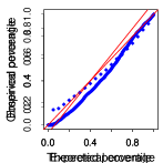
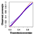
In Appendix A, we describe different diagnostic tests that can be used to more closely assess the quality of different models. Fig. 9, for example, shows quantile-quantile (Q-Q) plots of the SDSS data for NN_CS and Comb${}_{{CS}_{VS}}$. These plots tell us how well these density estimates actually fit the observed data.

(a) NN_CS

(b) Comb${}_{{CS}_{VS}}$

Figure 9: Quantile-quantile plots for (a) NN_CS and (b) Comb${}_{{CS}_{VS}}$, the combined model with selected covariates.

6 Application to Galaxy-Galaxy Lensing

By working with a probability distribution of the photometric redshift instead of a single best estimate, one can reduce systematic biases in cosmological analyses (Mandelbaum et al. 2008; Wittman 2009; Sheldon et al. 2012). In this section, we study the galaxy-galaxy weak-lensing application from Sheldon et al. (2012) and offer new insights on the proper use of redshift distributions in downstream analysis; i.e., when estimating functions $g(z)$ of an unknown redshift $z$.

Weak gravitational lensing is the slight deflection of photons from distant astronomical sources that occurs when they pass near massive “lenses” (e.g., galaxies or galaxy clusters) lying closer to us. Lensing acts to magnify the sizes of the distant sources as well as to distort their shapes. Cosmologists can use it to directly probe the distribution of dark matter, a form of matter that does not interact with light (hence the moniker “dark”) and which comprises $\approx$27% of the mass-energy of the Universe. The critical surface density $\Sigma(z_{l},z_{s})$ determines the lensing strength of a given lens-source pair (Mandelbaum et al., 2008). The goal in this example is to estimate $g_{l}(z_{s})=\Sigma^{-1}(z_{l},z_{s})$ for a source galaxy with unknown redshift $z_{s}$, assuming that the redshift $z_{l}$ of lens $l$ is known. A naive approach is to evaluate the function $g_{l}(\cdot)$ at a point estimate of the source galaxy redshift $z_{s}$; i.e., to compute $g_{l}(\widehat{z}_{s})=\Sigma^{-1}(z_{l},\widehat{z}_{s})$ where $\widehat{z}_{s}$ typically is an estimate of the regression ${{\mathbb{E}}}[Z|{\mathbf{x}}]$. However, because ${\mathbb{E}}[g_{l}(Z)|{\mathbf{x}}]\neq g_{l}({\mathbb{E}}[Z|{\mathbf{x}}])$, the estimator

$$\widehat{\Sigma^{-1}}(z_{l},z_{s}):=\int\Sigma^{-1}(z_{l},z)\widehat{f}(z|\mathbf{x})dz$$ (19)

usually yields better results if $\widehat{f}(z|\mathbf{x})$ is a good estimate of $f(z|{\mathbf{x}})$ (Sheldon et al., 2012). Note that even though we ultimately are interested in $g_{l}(z)$, there are clear advantages in estimating the photo-$z$ density $f(z|\mathbf{x})$ well — rather than just aiming for the best regression of $g_{l}(Z)$ on the photometric covariates ${\mathbf{x}}$. For example, the data set in this example includes $\approx 500{,}000$ lenses that each has a different function $g_{l}$, and future data sets will only increase in size. With a good density estimator $\widehat{f}(z|\mathbf{x})$, one can address several different inference problems with different $g_{l}$’s simultaneously as well as construct reliable predictive intervals for each function $g_{l}(Z)$ for new observations of $Z$.

Following Sheldon et al. (2012), we use data from the DEEP2 EGS Region (Weiner et al., 2005). In addition to the conditional density estimators in Sec. 5, we implement a nearest-neighbors density estimator with 7 neighbors (the value hand-picked by Sheldon et al. 2012 for this particular application), and photoz, which computes $\Sigma^{-1}(z_{l},\widehat{z}_{s})$ where $\widehat{z}_{s}$ is the nearest neighbor regression estimate of $z_{s}$. To assess the performance of these methods in galaxy-galaxy lensing, we use the two measures in Mandelbaum et al. (2008) called the lensing calibration bias and the variance ratio. Small values of bias and large values of variance ratio indicate good performance. We use 500 samples for training, 500 for validation, and 382 for testing.

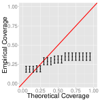
Fig. 10 shows the results. The nearest neighbor density estimator with 7 neighbors, NN-7, has a smaller calibration bias than NN with 27 neighbors, the value chosen via the technique described in the paper (see plot a). However, 7 neighbors leads to poor density estimates (see plot e). Series is the only estimator that returns both accurate parameter estimates for different values of $z_{l}$ and lenses $l$ (plots a and b), as well as accurate photo-$z$ density estimates (plots c and f). The other estimators do not have both of these properties simultaneously: depending on the chosen tuning parameter, either they have small bias but bad coverage (as NN-7), or good coverage but high bias (as NN) (see Appendix A for details on how the coverage is computed.).

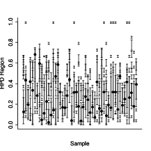
With conditional density estimates, we can also construct predictive density regions for the unknown redshift. The bottom panel in Fig. 10 shows the 95% Highest Predictive Density regions (HPD; see Appendix A for a definition) of the redshift for Series and NN. The former HPD region is typically more informative; the size of the HPD’s from Series are on average $\approx 75\%$ the size of those from NN.

(a) Bias

(b) Variance ratio

(c) Series

(d) NN

(e) NN-7

(f) Series

(g) NN

Figure 10: Lensing photo-$z$ calibration for DEEP2: Series returns parameter estimates with smaller biases and variances than the other approaches (see plots a and b). Using 7 neighbors for nearest neighbors as in Sheldon et al. (2012) yields similar performance in terms of bias; however, the value 7 was hand-picked for this specific task and results in poor density estimates (plot e). Series also yields more informative predictive intervals for redshifts than NN (plots f and g).

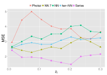
Finally, we note that estimating $f(z|\mathbf{x})$ by NN and then computing $\int g(z)\widehat{f}(z|\mathbf{x})dz$ is essentially equivalent to estimating ${\mathbb{E}}[g(Z)|\mathbf{x}]$ directly by performing nearest neighbors regression of $g(Z)$ on $\mathbf{x}$. In other words: for this particular application, NN-7 yields a good estimate of the regression of $g(Z)$ on ${\mathbf{x}}$, but not (as previously assumed) a reasonable estimate of photo-$z$.

7 Conclusions

Over the past 15 years, the number of applications for estimating photometric redshifts have grown rapidly, and today there exist a large number of techniques (or codes) for estimating redshifts; see, e.g., Dahlen et al. (2013) and references therein. With next-generation surveys, we also expect to have access to additional data (e.g., surface brightness or sizes of galaxies, Lima et al. 2008, or other magnitudes such as grizYJHKs, Oyaizu et al. 2008) which could potentially improve current photo-$z$ estimates. The value of our work is that it provides a principled framework for properly tuning and assessing different estimators, as well as methods for selecting covariates and for combining two or more estimators for optimal performance. In this paper, we also compared some new and existing estimators of importance weights and photometric redshift under different settings. We found that the nearest neighbors estimator from Cunha et al. (2009) is very effective for estimating importance weights, even when compared to state-of-the-art approaches for density ratio estimation from the machine learning literature. We introduced two new non-parametric conditional density estimators, kernel nearest neighbors (Section 5.2) and Series (Section 5.3), that both have better performance than the photo-z prediction method by Cunha et al. (2009).

Finally, although the scope of this paper is conditional density estimation, one can directly apply the proposed methods to the regression of functions of the photometric redshift, as the regression ${\mathbb{E}}[g(Z)|\mathbf{x}]=\int g(z)f(z|\mathbf{x})d\mathbf{x}$. The galaxy-galaxy lensing example in Sec. 6 clearly illustrates the importance of properly tuning and assessing photo-$z$ density estimators in down-stream cosmological analysis. In the example, our estimator yielded more accurate predictive regions for the redshift $z$, as well as better estimates of $g(z)$ for a range of different functions $g$, although we did not explicitly take $g$ into account in the optimization. We believe our proposed techniques will be valuable for astronomers and cosmologists carrying out next-generation surveys, where accurate photo-$z$ estimates will be needed within a range of different applications (and functions $g$).

Acknowledgments. We thank Jeffrey A. Newman for his insightful comments. We are also grateful to the referees and editors for the detailed comments that helped improve the paper. This work was partially supported by Conselho Nacional de Desenvolvimento Científico e Tecnológico (200959/2010-7), Fundação de Amparo à Pesquisa do Estado de São Paulo (2014/25302-2), the Estella Loomis McCandless Professorship, and NSF DMS-1520786.

SUPPLEMENTARY MATERIAL

We provide the data and code used in the paper as supplementary material.

Appendix A Diagnostic Tests for Conditional Density Estimation

The $L^{2}$ loss only conveys limited information on how well the final density estimates actually fit the observed data. Below we describe three diagnostic so-called goodness-of-fit tests that one can use to more closely assess the quality of different models; similar tests can be found in the time series literature (see, e.g., Corradi and Swanson 2006). Let $\widehat{F}_{z|\mathbf{x}_{i}}$ denote the estimated conditional cumulative distribution function for $z$ given $\mathbf{x}_{i}$. Then,

1. (Q-Q Plot) For every $c$ in a grid of values on $[0,1]$ and for every observation $i$ in the test spectroscopic sample, compute $Q_{i}^{c}=\widehat{F}_{z|\mathbf{x}_{i}}^{-1}(c)$. Define $\widehat{c}=\frac{1}{n}\sum_{i=1}^{n}\widehat{\beta}(x_{i}^{L}){\mathbb{I}}(z^{L}_{i}\leq Q_{i}^{c}).$ We plot the values of $\widehat{c}$ against the corresponding values of $c$. If the distributions $\widehat{F}_{z|\mathbf{x}}$ and $F_{z|\mathbf{x}}$ are similar, then the points in the Q-Q plot will approximately lie on the line $\widehat{c}=c$.

2. (P-value) For every test data point $i$, let $U_{i}=\widehat{F}_{z|\mathbf{x}_{i}}(Z_{i}).$ If the data are really distributed according to $\widehat{F}_{z|\mathbf{x}}$, then $U_{1},\ldots,U_{n}\overset{\mbox{\tiny{iid}}}{\sim}Unif(0,1)$. Hence, we compute the p-value for a Kolmogorov-Smirnoff test that compares the distributions of these statistics to the uniform distribution.

3. (Coverage Plot and HPD Regions) For every $\alpha$ in a grid of values in $[0,1]$ and for every spectroscopic data point $i$ in the test sample, let $A_{i}$ be a set such that $\int_{A_{i}}\widehat{f}(z|\mathbf{x}^{L}_{i})dz=\alpha.$ Here we choose the set $A_{i}$ with the smallest area: $A_{i}=\{z:f(z|{\mathbf{x}}_{i}^{L})>t\}$ where $t$ is such that $\int_{A_{i}}\widehat{f}(z|\mathbf{x}^{L}_{i})dz=\alpha$ (i.e., $A_{i}$ is a Highest Predictive Density region; HPD). Define $\widehat{\alpha}_{i}=\frac{1}{n}\sum_{i=1}^{n}\widehat{\beta}(x_{i}^{L}){\mathbb{I}}(z^{L}_{i}\in A_{i}).$ If the distributions $\widehat{F}_{z|\mathbf{x}}$ and $F_{z|\mathbf{x}}$ are similar, then $\widehat{\alpha}\approx\alpha$. Hence, we plot a graph of $\widehat{\alpha}$’s versus $\alpha$’s and assess how close they are to the line $\widehat{\alpha}=\alpha$. For each $\alpha$, we also include a $95\%$ confidence interval based on a normal approximation to the binomial distribution.

Appendix B Estimating Importance Weights

Some common approaches to estimating density ratios include direct basis expansions of the form $\widehat{\beta}(\mathbf{x})=\sum_{i=1}^{I}\widehat{\alpha_{i}}\lambda_{i}(\mathbf{x})$ [Kanamori et al., 2009, Sugiyama et al., 2008, Izbicki et al., 2014], kernel mean matching (KMM; Gretton et al. 2010), and various machine learning techniques (see, e.g., Bickel et al. 2009 and Margolis 2011 for a review). Astronomers have also themselves explored nearest neighbor-based techniques for reweighting non-representative training samples. In particular, Lima et al. [2008] and Cunha et al. [2009] have had success in photo-z estimation with the nearest-neighbor estimator

$$\widehat{\beta}(\mathbf{x})=\frac{1}{M}\frac{n_{L}}{n_{U}}\sum_{k=1}^{n_{U}}{\mathbb{I}}\left({\mathbf{x}}^{U}_{k}\in V_{\mathbf{x}}^{M}\right),$$ (20)

where

$$V_{\mathbf{x}}^{M}=\{\mathbf{y}\in\mathbb{R}^{d}:d(\mathbf{y},\mathbf{x})\leq d(\mathbf{x}^{L}_{(M)},\mathbf{x})\}$$

denotes the region of feature space with points that are closer to $\mathbf{x}$ than $\mathbf{x}^{L}_{(M)}$, the $M$th nearest neighbor of $\mathbf{x}$ among labeled data, is to ${\mathbf{x}}$. This estimator has also been used in the machine learning literature [Loog, 2012], although only for the case $M=1$.

Model Selection and Tuning of Parameters. To select the best method for estimating $\beta({\mathbf{x}})$, we need to specify an appropriate loss function. Our ultimate goal is good photo-$z$ prediction for new unlabeled data. If we use importance weighting according to Eq. 3, then we need good estimates of $\beta(\mathbf{x})$ at the labeled points, or more generally, in regions where the density of labeled points is large. Hence, we define the loss function according to Eq. 4, which is weighted with respect to ${\mathbb{P}}_{L}$. (These weights are later used in Eq. 9 to estimate the ${\mathbb{P}}_{U}$-weighted loss in Eq. 8 for CDE.)

References

- Aihara et al. [2011] H. Aihara et al. The eighth data release of the Sloan Digital Sky Survey: first data from SDSS-III. The Astrophysical Journal Supplement Series, 193(2):29, 2011.
- Ball and Brunner [2010] N.M. Ball and R.J. Brunner. Data mining and machine learning in astronomy. International Journal of Modern Physics D, 19:1049–1106, 2010.
- Bickel et al. [2009] S. Bickel, M. Brückner, and T. Scheffer. Discriminative learning under covariate shift. Journal of Machine Learning Research, 10:2137–2155, 2009.
- Corradi and Swanson [2006] V. Corradi and N. R. Swanson. Predictive density evaluation. In Handbook of Economic Forecasting. North-Holland, 2006.
- Cunha et al. [2009] C.E. Cunha, M. Lima, H. Oyaizu, J. Frieman, and H. Lin. Estimating the redshift distribution of photometric galaxy samples — II. Applications and tests of a new method. Monthly Notices of the Royal Astronomical Society, (396):2379–2398, 2009.
- Dahlen et al. [2013] T. Dahlen, B. Mobasher, S. M. Faber, H. C. Ferguson, G. Barro, S. L. Finkelstein, K. Finlator, A. Fontana, R. Gruetzbauch, S. Johnson, et al. A critical assessment of photometric redshift methods: a CANDELS investigation. The Astrophysical Journal, 775(2):93, 2013.
- Fernández-Soto et al. [1998] A. Fernández-Soto, K. M. Lanzetta, and A. Yahil. A new catalog of photometric redshifts in the Hubble Deep Field. The Astrophysical Journal, 513:34–50, 1998.
- Gretton et al. [2010] A. Gretton, A. Smola, J. Huang, M. Schmittfull, K. Borgwardt, and B. Schölkopf. Covariate shift by kernel mean matching. In J. Quionero-Candela, M. Sugiyama, A. Schwaighofer, and N. D. Lawrence, editors, Dataset Shift in Machine Learning, chapter 8. The MIT Press, 2010.
- Hall [1987] P. Hall. On kullback-leibler loss and density estimation. The Annals of Statistics, pages 1491–1519, 1987.
- Hastie et al. [2009] T. Hastie, R. Tibshirani, and J. H. Friedman. The elements of statistical learning: data mining, inference, and prediction. Springer, 2009.
- Izbicki and Lee [2015] R. Izbicki and A. B. Lee. Nonparametric conditional density estimation in a high-dimensional regression setting. Journal of Computational and Graphical Statistics, (just accepted), 2015.
- Izbicki et al. [2014] R. Izbicki, A.B. Lee, and C. M. Schafer. High-dimensional density ratio estimation with extensions to approximate likelihood computation. Journal of Machine Learning Research W&CP (AISTATS track), 33, 2014.
- Kanamori et al. [2009] T. Kanamori, S. Hido, and M. Sugiyama. A least-squares approach to direct importance estimation. Journal of Machine Learning Research, 10:1391–1445, 2009.
- Kanamori et al. [2012] T. Kanamori, T. Suzuki, and M. Sugiyama. Statistical analysis of kernel-based least-squares density-ratio estimation. Machine Learning, 86(3):335–367, 2012.
- Kind and Brunner [2013] M. C. Kind and R. J. Brunner. Tpz: photometric redshift pdfs and ancillary information by using prediction trees and random forests. Monthly Notices of the Royal Astronomical Society, 432(2):1483–1501, 2013.
- Koenker [2005] R. Koenker. Quantile Regression. Cambridge University Press, 2005.
- Kremer et al. [2015] J. Kremer, F. Gieseke, K. S. Pedersen, and C. Igel. Nearest neighbor density ratio estimation for large-scale applications in astronomy. Astronomy and Computing, 2015.
- Lima et al. [2008] M. Lima, C.E. Cunha, H. Oyaizu, J. Frieman, H. Lin, and E. Sheldon. Estimating the redshift distribution of photometric galaxy samples. Monthly Notices of the Royal Astronomical Society, (390):118–130, 2008.
- Loog [2012] M. Loog. Nearest neighbor-based importance weighting. In IEEE International workshop on machine learning for signal processing, 2012.
- Mandelbaum et al. [2008] R. Mandelbaum, U. Seljak, C. M. Hirata, S. Bardelli, M. Bolzonella, Bongiorno A., M. Carollo, T. Contini, C. E. Cunha, B. Garilli, A. Iovino, P. Kampczyk, J.P. Kneib, C. Knobel, D. C. Koo, F. Lamareille, O. Le Fevre, J.F. Leborgne, S. J. Lilly, C. Maier, V. Mainieri, M. Mignoli, J. A. Newman, P. A. Oesch, E. Perez-Montero, E. Ricciardelli, M. Scodeggio, J. Silverman, and L. Tasca. Precision photometric redshift calibration for galaxy-galaxy weak lensing. Monthly Notices of the Royal Astronomical Society, (386):781–806, 2008.
- Margolis [2011] A. Margolis. A literature review of domain adaptation with unlabeled data. March 2011.
- Minh et al. [2006] H. Q. Minh, P. Niyogi, and Y. Yao. Mercer’s theorem, feature maps, and smoothing. In Learning Theory, 19th Annual Conference on Learning Theory, 2006.
- Moreno-Torres et al. [2012] J. G. Moreno-Torres, T. Raeder, R. Alaíz-Rodríguez, N. V. Chawla, and F. Herrera. A unifying view on dataset shift in classification. Pattern Recognition, 45(1):521–530, 2012.
- Oyaizu et al. [2008] H. Oyaizu, M. Lima, C.E. Cunha, H. Lin, and J. Frieman. Photometric redshift error estimators. The Astrophysical Journal, (689):709–720, 2008.
- Quionero-Candela et al. [2009] J. Quionero-Candela, M. Sugiyama, A. Schwaighofer, and N. D. Lawrence. Dataset Shift in Machine Learning. The MIT Press, 2009.
- Rubin [1976] D. B. Rubin. Inference and missing data. Biometrika, 63(3):581–592, 1976.
- Sheldon et al. [2012] E. S. Sheldon, C. E. Cunha, R. Mandelbaum, J. Brinkmann, and B. A. Weaver. Photometric redshift probability distributions for galaxies in the SDSS DR8. The Astrophysical Journal Supplement Series, 201(2):32, 2012.
- Shimodaira [2000] H. Shimodaira. Improving predictive inference under covariate shift by weighting the log-likelihood function. Journal of Statistical Planning and Inference, 90(2):227–244, 2000.
- Springel et al. [2006] V. Springel, C. S. Frenk, and S. D.M. White. The large-scale structure of the universe. Nature, 440:1137–1144, 2006.
- Sugiyama et al. [2008] M. Sugiyama, T. Suzuki, S. Nakajima, H. Kashima, P. Bünau, and M. Kawanabe. Direct importance estimation for covariate shift adaptation. Annals of the Institute of Statistical Mathematics, 60(4):699–746, 2008.
- Wasserman [2006] L. Wasserman. All of Nonparametric Statistics. Springer-Verlag New York, Inc., 2006.
- Weiner et al. [2005] B. J. Weiner, A. C. Phillips, S.M. Faber, C. N.A. Willmer, N. P. Vogt, et al. The DEEP groth strip galaxy redshift survey. III. Redshift catalog and properties of galaxies. The Astrophysical Journal, 620(2):595, 2005.
- Wittman [2009] D. Wittman. What lies beneath: Using p(z) to reduce systematic photometric redshift errors. The Astrophysical Journal Letters, 700(2), 2009.
- York et al. [2000] D. G. York, J. Adelman, J. E. Anderson Jr, S. F. Anderson, J. Annis, N. A. Bahcall, J. A. Bakken, R. Barkhouser, S. Bastian, E. Berman, et al. The Sloan Digital Sky Survey: Technical summary. The Astronomical Journal, 120(3):1579, 2000.
- Zhao and Liu [1985] L. Zhao and Z. Liu. Strong consistency of the kernel estimators of conditional density function. Acta Mathematica Sinica, 1(4):314–318, 1985.
- Zheng and Zhang [2012] H. Zheng and Y. Zhang. Review of techniques for photometric redshift estimation. In Software and Cyberinfrastructure for Astronomy II, volume 8451, 2012.