Liquid and solid phases of ³He on graphite

Abstract

Recent heat-capacity experiments show quite unambiguously the existence of a liquid ³He phase adsorbed on graphite. This liquid is stable at an extremely low density, possibly one of the lowest found in Nature. Previous theoretical calculations of the same system, and in strictly two dimensions, agree with the result that this liquid phase is not stable and the system is in the gas phase. We calculated the phase diagram of normal ³He adsorbed on graphite at $T=0$ using quantum Monte Carlo methods. Considering a fully corrugated substrate we observe that at densities lower that 0.006 Å^-2 the system is a very dilute gas, that at that density is in equilibrium with a liquid of density 0.014 Å^-2. Our prediction matches very well the recent experimental findings on the same system. On the contrary, when a flat substrate is considered, no gas-liquid coexistence is found, in agreement with previous calculations. We also report results on the different solid structures, and the corresponding phase transitions that appear at higher densities.

Recent heat capacity measurements of ³He adsorbed on graphite by Sato et al. fukuyama ; fukuyama1 have shown that its monolayer is a stable liquid in the density range $0.006$-$0.009$ Å^-2. One of the most interesting aspects of this phase is its extremely low density, with interparticle distances as large as 10 Å, which could constitute one of the lowest-density stable liquids in nature. This new finding has re-opened an old issue that has been under discussion for more than thirty years, i.e., the nature (gas or liquid) of two-dimensional (2D) ³He gasparinip ; smart . Previous experiments showed contradictory results due in part to the different setups and employed substrates gasparini ; godfrin ; greywall ; hallock . Now, the new data from Ref. fukuyama on a clean graphite substrate seem to incline the debate towards the confirmation of this liquid phase existence.

On the theoretical side, there is a broad consensus on the gas character of strictly 2D ³He novaco ; miller ; hnc ; chester ; grau . However, the practical need of a substrate to actually realize the ³He monolayer could modify this result. Previous attempts to calculate the properties of the adsorbed monolayer in a strongly attractive substrate such as graphite arrived to the same result. In Ref. bonin , it is shown that the possibility of ³He atoms moving perpendicularly to the surface leads to a stable liquid phase when the substrate is weakly attractive, as on some alkali metal surfaces. This is probably expected because the system goes from a 2D film to a three-dimensional (3D) configuration where liquid ³He is the ground-state phase.

In this work, we concerned ourselves with the adsorption of ³He on a clean surface of graphite, trying to reproduce the recent experimental findings of Sato et al.  fukuyama Our goal was to bridge the discrepancy between the strictly 2D calculations and the experimental data by improving the theoretical description of the system. Since considering a quasi-two dimensional flat adsorbent is clearly not enough for graphite bonin , we included the effects of the substrate corrugation on the behavior of the adsorbate, in line with what has been done previously for ⁴He on the same system yo ; yo3 ; yo2 ; manu1 ; manu2 ; manu3 ; manu4 ; manu5 . We found that a corrugated surface is the missing ingredient to reconcile the experimental and theoretical data. In addition, this approach allows us also to calculate the entire phase diagram of ³He on graphite, including the commensurate solids that cannot appear in a strictly 2D model.

Given the low temperatures involved in the experiments (of the order of mK), it is reasonable to think that the ground state of ³He on graphite is a reasonable description of the system under consideration. To obtain it, we have to solve the Schrödinger equation corresponding to the many-body Hamiltonian,

$$H=\sum_{i=1}^{N}\left[-\frac{\hbar^{2}}{2m}\nabla^{2}+V_{\text{ext}}(x_{i},y_{i},z_{i})\right]+\sum_{i<j}^{N}V_{\text{He-He}}(r_{ij}),$$ (1)

where $x_{i},y_{i}$ and $z_{i}$ are the coordinates for each of the $N$ ³He atoms, and $m$ their mass. Following Ref. yo , graphite was modeled by a set of eight graphene layers separated $3.35$ Å in the $z$ direction and stacked in the A-B-A-B way typical of this compound. All the individual carbon atoms in each layer were considered. $V_{\text{ext}}(x_{i},y_{i},z_{i})$ was the sum of all the C-He atomic interactions, calculated using the Carlos and Cole anisotropic potential carlosandcole , which has been widely used in calculations of ⁴He adsorbed on graphite. $V_{\text{He-He}}(r)$ is the standard Aziz potential aziz , that depends on the distance $r_{ij}$ between ³He atoms.

To solve the Schrödinger equation describing the system, we used the diffusion Monte Carlo (DMC) method. For a set of bosons, DMC allows us to obtain exactly the energy of their ground state, within the statistical uncertainties derived from the stochastic nature of the method. However, when we deal with fermions, as in the present case, the sign problem makes an exact calculation not possible. We follow the usual approach in which one imposes that the nodal surface is the one of the trial wavefunction used as guiding function in the DMC algorithm hammond . This approximation is known as fixed-node method (FN) and provides an upper bound to the exact ground-state energy of the system. We chose as a trial wavefunction

$$\Phi({\bf r_{1},r_{2},...,r_{N}})=D^{\uparrow}D^{\downarrow}\prod_{i<j}\exp\left[-\frac{1}{2}\left(\frac{b_{\rm He-He}}{r_{ij}}\right)^{5}\right]$$ (2)

where ${\bf r_{1},r_{2},...,r_{N}}$ are the helium coordinates. The parameter $b_{\rm He-He}$ in the Jastrow part of Eq. (2) was taken to be $2.96$ Å, as in a purely two-dimensional system grau . $D^{\uparrow}$ and $D^{\downarrow}$ are Slater determinants that depend on the coordinates of the spin-up and spin-down atoms, respectively. We considered always an unpolarized phase, $N_{\uparrow}=N_{\downarrow}=N/2$. The single-particle functions entering those determinants, $\psi({\bf r_{i}})$, were the solutions of the Schrödinger equation derived from the one-body Hamiltonian resulting of dropping the interparticle interaction [last term in Eq. (1)]. Since $V_{\text{ext}}(x_{i},y_{i},z_{i})$ has the periodicity of the underlying substrate, we can invoke Bloch’s theorem to write ashcroft

$$\psi({\bf r_{i}})=u({\bf r_{i}})_{\bf k}\exp(ik_{x}x_{i}+ik_{y}y_{i}),$$ (3)

where $u({\bf r_{i}})_{\bf k}$ obeys the Born-von Karman periodic boundary conditions (in 2D) with respect to the unit cell whose replication defines the graphite structure. We chose as unit cell one whose surface is 2.46 $\times$ 4.26 Ų, that includes four carbon atoms in its upper layer (the ones that form the characteristic hexagon of a honeycomb arrangement). In general, $u({\bf r_{i}})_{\bf k}$ depends on the reciprocal vector k = $(k_{x},k_{y})$. Here, $k_{x}$= $2\pi n/L_{x}$ and $k_{y}$= $2\pi m/L_{y}$, where $L_{x}$ and $L_{y}$ are the sides of our rectangular simulation cell, $n$ and $m$ being integers. To describe the gas-liquid transition we used a cell of 73.79 $\times$ 72.42 Ų, i.e., with a surface 30 $\times$ 17 times that of the unit cell defined above. Introducing Eq. (3) into the Hamiltonian (1), the one-body Schrödinger equation transforms into

$$Hu({\bf r_{i}})_{\bf k} = \left(\frac{\hbar^{2}}{2m}\left(\frac{1}{i}{\bf\nabla+k}\right)^{2}+V_{ext}(x_{i},y_{i},z_{i})\right)u({\bf r_{i}})_{\bf k}$$ (4)

$$= E_{\bf k}u({\bf r_{i}})_{\bf k}$$

We solved numerically this complex eigenvalue-eigenvector problem by expanding

$$u({\bf r_{i}})_{\bf k}=\frac{\sqrt{2}}{\sqrt{(l_{x}l_{y}l_{z})}}\sum_{j_{1}=-n_{x}}^{n_{x}}\sum_{j_{2}=-n_{y}}^{n_{y}}\sum_{j_{3}=1}^{n_{z}}c_{j_{1}j_{2}j_{3}}$$ (5)

$$\times\exp[i(j_{1}g_{x}x_{i}+j_{2}g_{y}y_{i})]\sin(j_{3}g_{z}(z_{i}-z_{0}))$$

and solving for the $c_{j_{1}j_{2}j_{3}}$ coefficients. Here, $n_{x}$ = 4, $n_{y}$=6, and $n_{z}$ = 30; $g_{x}$ = $2\pi/l_{x}$, $g_{y}$ = $2\pi/l_{y}$, and $g_{x}$ = $\pi/l_{z}$; $l_{x}$ = 2.46 Å, $l_{y}$= 4.26 Å and $l_{z}$ = 8-$z_{0}$ Å ($z_{0}$ = 1.5 Å). The solutions of Eq. (4) were not restricted to be real. We used the number of functions necessary to assure us an energy cutoff of 0.001 K. The ground state of a single ³He atom obtained using this method was $E_{(0,0)}$ = $E_{0}$ = -135.771 $\pm$ 0.001 K. A plot of $u(x,y,z=2.88)_{(0,0)}$ is displayed in Fig. 1, showing the corrugation of the ground state. That value of $z$ is the one for which the value of the wavefunction is maximum.

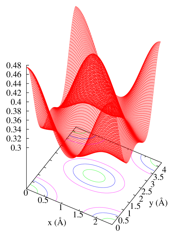
Figure 1: (Color online) Plot of $u(x,y,z=2.88)_{(0,0)}$ with its corresponding contour map showing the corrugation of the one-particle part of the trial wavefunction.

Using the method described above, we obtained the $u({\bf r_{i}})_{\bf k}$ functions corresponding to the first band of the periodic potential created by the graphite substrate. With them, and using Eq. (3), we can construct the one-body functions entering in the Slater determinants in Eq. (2). However, we found that, at least for the first-band functions we needed, all the $u({\bf r_{i}})_{\bf k}$ were real and independent of $\bf{k}$ within the numerical errors derived from the procedure. This transforms Eq. (2) into

$$\Phi({\bf r_{1},r_{2},...,r_{N}})=D^{\prime\uparrow}D^{\prime\downarrow}\prod_{i}u({\bf r_{i}})\prod_{i<j}\exp\left[-\frac{1}{2}\left(\frac{b_{\rm He-He}}{r_{ij}}\right)^{5}\right]$$ (6)

with $D^{\prime\uparrow}$ and $D^{\prime\downarrow}$ the plane-wave Slater determinants of the strictly 2D system grau ; bonin . We also shifted the coordinates entering these Slater determinants by introducing backflow correlations in the standard way

$$\tilde{x}_{i} = x_{i}+\lambda\sum_{j\neq i}\exp[-(r_{ij}-r_{b})^{2}/\omega^{2}](x_{i}-x_{j})$$ (7)

$$\tilde{y}_{i} = y_{i}+\lambda\sum_{j\neq i}\exp[-(r_{ij}-r_{b})^{2}/\omega^{2}](y_{i}-y_{j})\ .$$ (8)

We tested that the best parameters in those last equations were those corresponding to the full three-dimensional homogeneous system casulleras , i.e., $\lambda=0.35$; $\omega=1.38$ Å, and $r_{b}=1.89$ Å, instead of the ones corresponding to a pure 2D grau . We made standard checks on the mean population of configurations and time step to reduce any systematic bias to the level of the statistical noise. Also, we included standard finite-size corrections to the energy coming from both the discretization of the Fermi sphere and to the potential energy contributions beyond the size of the simulation box.

The results of the DMC simulations that consider a fully corrugated C-He potential are displayed in Fig. 2 as full squares. As indicated above, we considered a simulation cell of 73.79 $\times$ 72.42 Ų including up to 130 atoms, half of them with spin up, and the other half with spin down. In that figure, it is also included the strictly 2D results of Ref. grau, as a full line. To afford a comparison between the two sets of data, in the first case we subtracted the energy in the infinite dilution limit ($E_{0}$) to the energy per particle ($E/N$). What we see is that, apart from the limit when $\rho\rightarrow 0$, there is a sizeable difference between both sets of data, including an a significant energy stabilization for the full quasi-two-dimensional systems for $\rho>0.005$ Å^-2.

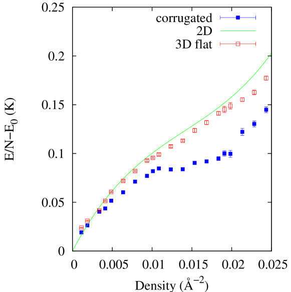
Figure 2: (Color online) Energy per ³He atom (E/N) versus surface density for corrugated (full symbols) and flat (open symbols) graphite. In both cases, we subtracted the energy in the infinite dilution limit, $E_{0}$, to allow for a better comparison. The equation of state of a pure 2D liquid given in Ref. grau, is also given for comparison.

To check if that decrease in the energy per particle is due simply to the inclusion of the additional degree of freedom in the $z$ axis or there is something else, we performed an additional FN-DMC calculation using an averaged-over version of the external potential of Eq. (1) in the $z$ axis. Using a similar procedure to the one outlined above, we obtained $u(z_{i})$, the one-body part of the trial function. The open symbols in Fig. 2 are the results of that additional FN-DMC calculation. Here, as before, the energy in the infinite dilution limit corresponding to the adsorption of a single ³He atom on that flat graphite model was subtracted. Its absolute value was slightly smaller than that of the fully corrugated case ($E_{0}=-133.585\pm 0.001$ K). For that second case, the energies per particle are much closer to the ones corresponding to a pure 2D system. This is in line with the prediction of Ref. bonin , but contradicts the results of Ref. brami , where only smoothed-out substrates were studied.

In Fig. 3, we show the same corrugated data as in Fig. 2, but as a function of the inverse of the ³He density. At first sight, we can see that there is a non-stability zone around a surface per particle of around 100 Ų. In that figure it is also displayed the double-tangent Maxwell construction line (see Ref. chandler for details about its construction). This allows us to see that there is indeed a first-order phase transition between a dilute gas of density $0.006\pm 0.002$ Å^-2, and a liquid one of $0.014\pm 0.002$ Å^-2. We can assign tentatively that transition to the gas-liquid equilibrium suggested in Ref. fukuyama for ³He on clean graphite. We have to stress also that we did not use different trial wavefunctions for gas and liquid phases, the instability appearing naturally when we increase the helium density.

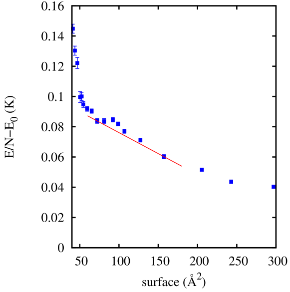
Figure 3: (Color online) Full corrugated results for the energy per ³He atom as a function of the surface per particle. The line stands for the double-tangent Maxwell construction to determine the equilibrium densities of the gas and liquid phases.

If we increase further the amount of helium adsorbed, the system will undergo another phase transition, in this case to a $\sqrt{3}\times\sqrt{3}$ registered phase, similar to that of ⁴He on graphite. This is illustrated in Fig. 4. There, we plot the energy per particle for a liquid (open squares), an incommensurate solid (open circles), and several registered structures (full symbols). The calculations for the liquid phase, quite beyond the transition point, were done using the same procedure outlined above but using a smaller simulation cell, one with a surface of 44.28 $\times$ 42.6 Å^-2. To model the solid structures, we followed Ref. yo, , and multiplied the trial function of Eq. (2) by a Nosanow factor,

$$\prod_{i}\exp\{-a[(x_{i}-x_{\rm site})^{2}+(y_{i}-y_{\rm site})^{2}]\}\ ,$$ (9)

where $x_{\rm site},y_{\rm site}$ are the coordinates of the crystallographic positions of the solid structures, and $a$ was variationally optimized ($a$=0.24 Å^-2 for all the lattices). To establish the boundaries between the liquid phase and the $\sqrt{3}\times\sqrt{3}$ commensurate structure, we would have to do another double-tangent Maxwell construction. We proceeded in the same way as in previous literature, by drawing the line with the smallest negative slope that goes from the inverse of the solid density and intercepts the liquid equation of state. We found that the $\sqrt{3}\times\sqrt{3}$ solid is in equilibrium with a liquid of density 0.039 $\pm$ 0.001 Å^-2, i.e., the stability range of the liquid is from 0.014 $\pm$ 0.002 Å^-2 to 0.039 $\pm$ 0.001 Å^-2. The latter value is in good agreement with the experimental upper value for a liquid phase found for a three-layer ³He system godfrin . The smallest value of the interval is compatible with the experimental lower value for the same system fukuyama1 .

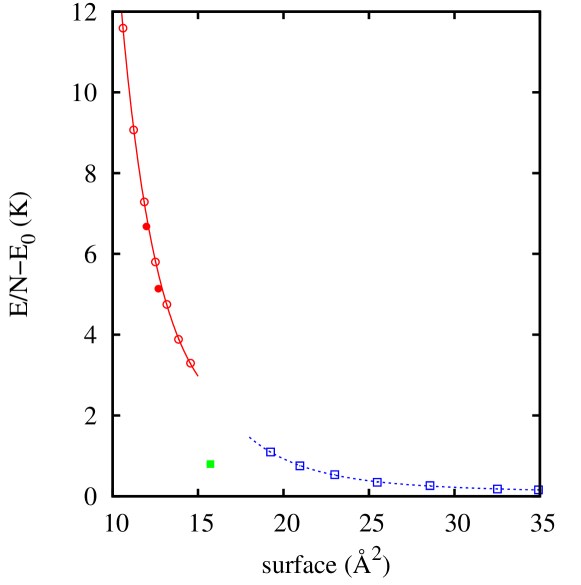
Figure 4: (Color online) Same as for Fig 3 but for higher values of the surface per particle. Open squares, liquid phase; open circles, incommensurate solid; full square, $\sqrt{3}\times\sqrt{3}$ phase; full circles, $31/75$ (lower one) and $7/16$ (upper one), registered phases. The error bars are of the size of the symbols and not displayed for simplicity. The guides are mere guides-to-the-eye.

The full symbols in Fig. 4 correspond to two commensurate solids already considered for quantum species on graphite, the $31/75$ ($\rho$ = 0.0789 Å^-2, found for D₂ frei ; yo4 ), and the $7/16$ ($\rho$ = 0.0835 Å^-2, proposed to be stable by Corboz et al. for ⁴He corboz ). As one can see in that figure, we found that those registered solids are slightly more stable than the corresponding incommensurate (IC) solids of the same density. In particular, the energies per atoms are: $E_{31/75}$ = -130.63 $\pm$ 0.02 K versus $E_{\text{IC}}$ = -130.30 $\pm$ 0.01 K, and $E_{7/16}$ = -129.09 $\pm$ 0.02 K versus $E_{\text{IC}}$ = -129.00 $\pm$ 0.02 K. This means that if we increase the density beyond the one corresponding to the $\sqrt{3}\times\sqrt{3}$ structure (0.0636 Å^-2), the system will undergo a first-order phase transition to a registered $31/75$ structure that, on further increase will transform into a $7/16$ one. Obviously, these latter phase transitions are predicted to exist in the limit of zero temperature and they could be smoothed out if the temperature is not low enough due to the small energy differences here obtained. At higher densities, there is a last transition into an incommensurate triangular solid. Another Maxwell construction using the data shown in Fig. 4 allowed us to obtain that the lower density limit of this phase is 0.089 $\pm$ 0.005 Å^-2.

The results presented allow us to give a coherent picture that can incorporate all the experimental results on ³He on graphite. The very dilute density for the liquid phase found in Refs. gasparini ; fukuyama ($\sim$ 0.006 Å^-2) is compatible with our lower limit for the gas-liquid transition. This means that for ranges 0.006 Å${}^{-2}<\rho<$ 0.014 Å^-2 the system will separate itself into a very dilute gas phase and puddles of liquid of density 0.014 Å^-2, in the right proportions to produce the density we considered within that interval. So, from 0.006 Å^-2 up, we will have part of the surface covered by a liquid. That coverage will be complete when the overall ³He density is $\rho$ = 0.014 Å^-2, in which all graphite will be coated by an homogeneous liquid. That liquid will be stable up to 0.039 $\pm$ 0.001 Å^-2, in line with the results of Ref. godfrin, . On the other hand, we see that ³He presents two new stable registered phases at relatively high densities. The only experimental support for the first one ($31/75$) are the calorimetric measurements of Greywall greywall , in with a ³He first-layer solid phase on graphite at $\rho$ = 0.076 Å^-2 is considered. However, the phase proposed is a $2/5$ one, that we found to be unstable with respect to an incommensurate triangular solid of the same density. Our results show that the main, and forgot up to now, ingredient to satisfactorily describe the monolayer of ³He on graphite is the use of a realistic C-He interaction instead of smoothed or averaged surface-helium potentials.

- (1) D. Sato, K. Naruse, T. Matsui, and H. Fukuyama, Phys. Rev. Lett. 109, 235306 (2012).
- (2) D. Sato, T. Tsuji, S. Takayoshi, K. Obata, T. Matsui, and H. Fukuyama, J. Low. Temp. Phys. 158, 201 (2010).
- (3) Francis M. Gasparini, Physics 5, 136 (2012).
- (4) Ashley G. Smart, Phys. Today 66, 16 (2013).
- (5) B. K. Bhattacharyya and F.M. Gasparini, Phys. Rev. B 31, 2719 (1985).
- (6) H. Godfrin, R. E. Rapp, K. D. Morhard, J. Bossy, and C. Bauerle, Phys. Rev. B 49, 12377 (1994).
- (7) D. S. Greywall, Phys. Rev. B 47, 309 (1993).
- (8) Pei-Chung Ho and R. B. Hallock, Phys. Rev. Lett. 87, 135301 (2001).
- (9) V. Grau, J. Boronat, and J. Casulleras. Phys. Rev. Lett. 89, 045301 (2002).
- (10) A.D. Novaco and C.E. Campbell, Phys. Rev. B. 11, 2525 (1975).
- (11) M.D. Miller and L.H. Nosanov, J. Low. Temp. Phys. 32, 145 (1978).
- (12) C. Um, J. Kahng, Y. Kim, T. F. George, and L. N. Pandey, J. Low Temp. Phys. 107, 283 (1997).
- (13) B. Krishnamachari and G. V. Chester. Phys. Rev. B 59, 8852 (1999).
- (14) M. Ruggeri, S. Moroni, and M. Boninsegni. Phys. Rev. Lett. 111, 045303 (2013).
- (15) M. C. Gordillo and J. Boronat, Phys. Rev. Lett. 102, 085303 (2009).
- (16) M. C. Gordillo, Phys. Rev. B 89, 155401 (2014).
- (17) M. C. Gordillo, C. Cazorla, and J. Boronat. Phys. Rev. B 83, 121406(R) (2011).
- (18) M. Pierce and E. Manousakis, Phys. Rev. Lett. 81 , 156 (1998).
- (19) M. Pierce and E. Manousakis, Phys. Rev. B 59, 3802 (1999).
- (20) M. Pierce and E. Manousakis, Phys. Rev. Lett. 83, 5314 (1999).
- (21) M. E. Pierce and E. Manousakis, Phys. Rev. B 62, 5228 (2000).
- (22) M. E. Pierce and E. Manousakis, Phys. Rev. B 63, 144524 (2001).
- (23) W. E. Carlos and M. W. Cole, Surf. Sci. 91, 339 (1980).
- (24) R.A. Aziz, F. R. W. McCourt, and C.C. K. Wong, Mol. Phys. 61, 1487 (1987).
- (25) B. L. Hammond, W.A. Lester, Jr., and P.J. Reynolds Monte Carlo Methods in Ab Initio Quantum Chemistry (World Scientific, Singapore, 1994).
- (26) N.W. Ascroft and N.D. Mermin Solid State Physics (Saunders College Publishing, Orlando, 1976).
- (27) J. Casulleras and J. Boronat. Phys. Rev. Lett. 84, 3121 (2000).
- (28) B. Brami, F. Joly, and C. Lhuillier, J. Low Temp. Phys. 94 63 (1994).
- (29) D. Chandler, Introduction to modern statistical mechanics, (Oxford University Press, Oxford, 1987).
- (30) P. Corboz, M. Boninsegni, L. Pollet, and M. Troyer, Phys. Rev. B 78, 245414 (2008).
- (31) H. Freimuth, H. Wiechert, H. P. Schildberg, and H. J. Lauter, Phys. Rev. B. 42, 587 (1990).
- (32) C. Carbonell-Coronado, M. C. Gordillo. Phys. Rev. B 85, 155427 (2012).
- (33) J. Boronat and J. Casulleras, Phys. Rev. B 49, 8920 (1994).