Linear structures in nonlinear optimal control

Abstract

We investigate optimal control of dynamical systems which are affine, i.e., linear in control, but nonlinear in state. The control task is to enforce the system state to follow a prescribed desired trajectory as closely as possible, a task also known as optimal trajectory tracking. To obtain well-behaved solutions to optimal control, a regularization term with coefficient $\varepsilon$ must be included in the cost functional. Assuming $\varepsilon$ to be small, we reinterpret affine optimal control problems as singularly perturbed differential equations. Performing a singular perturbation expansion, approximations for the optimal tracking of arbitrary desired trajectories are derived. For $\varepsilon=0$, the state trajectory may become discontinuous, and the control may diverge. On the other hand, the analytical treatment becomes exact. We identify the conditions leading to linear evolution equations. These result in exact analytical solutions for an entire class of nonlinear trajectory tracking problems. The class comprises, among others, mechanical control systems in one spatial dimension and the FitzHugh-Nagumo model with a control acting on the activator.

Introduction.

In principle, a controlled dynamical systems can be considerably simpler than the corresponding uncontrolled system. Consider Newton’s equation of motion (EOM), cast in form of a two-dimensional dynamical system, for a point particle with unit mass, position $x$, and velocity $y$. Under the influence of an external force $R$ and a control force $bu$, the EOM read

$$\dot{x} =y, \dot{y} =R\left(x,y\right)+b\left(x,y\right)u.$$ (1)

While no simple analytical expression for the solution exists for the uncontrolled system with $u\equiv 0$, assuming that $u$ is a feedback control signal renders a linearization of Eq. (1) possible. Indeed, for $b\left(x,y\right)\neq 0$, we may introduce a new control signal $v$ by $u=\frac{1}{b\left(x,y\right)}\left(v-R\left(x,y\right)\right)$ such that the new controlled system is linear, $\dot{x}=y,\,\dot{y}=v$. This technique is called feedback linearization and is applicable, in a more sophisticated fashion involving an additional state transformation, to a huge class of dynamical systems Khalil (2001). The resulting linear structure facilitates the application of a multitude of solution and analysis techniques, which are not available in the nonlinear case Chen (1998). Contrary to the more familiar approximate linearizations applied e.g. to study of the linear stability of attractors, feedback linearization is an example of an exact linearization. The question emerges if exact linearizations are exclusive to systems with feedback control.

In this letter, we demonstrate the possibility of linear structures in optimal control, which may or may not be a feedback control. As a result, the controlled state as well as the control signal are given as the solution to linear differential and algebraic equations. The finding enables the exact analytical solution of an entire class of nonlinear optimally controlled dynamical systems, including but not limited to all models of the form Eq. (1). While stabilizing feedback control of unstable attractors received much attention by the physics community Bechhoefer (2005), especially in the context of chaos control Ott et al. (1990), optimality of these methods is rarely investigated. Numerical solutions of optimal control problems are computationally expensive, which often prevents real time applications. Particularly optimal feedback control suffers from the ’curse of dimensionality’ Bellman (2003). On the other hand, analytical methods are largely restricted to linear systems which lack e.g. limit cycles and chaos. The approach presented here opens up a way to circumvent such problems.

Trajectory tracking aims at enforcing, via a vector of control signals $\boldsymbol{u}\in\mathbb{R}^{p}$, a system state $\boldsymbol{x}\in\mathbb{R}^{n}$ to follow a prescribed desired trajectory $\boldsymbol{x}_{d}\in\mathbb{R}^{n}$ as closely as possible within a time interval $t_{0}\leq t\leq t_{1}$. The distance between $\boldsymbol{x}$ and $\boldsymbol{x}_{d}$ in function space can be measured by the functional $\mathcal{J}=\frac{1}{2}\intop_{t_{0}}^{t_{1}}dt\left(\boldsymbol{x}-\boldsymbol{x}_{d}\right)^{2}$. $\mathcal{J}$ vanishes if and only if $\boldsymbol{x}=\boldsymbol{x}_{d}$, in which case we call $\boldsymbol{x}_{d}$ an exactly realizable desired trajectory Löber (2016, 2015). If $\boldsymbol{x}_{d}$ is not exactly realizable, we can formulate trajectory tracking as an optimization problem. The control task is to minimize the quadratic cost functional

$$\mathcal{J} =\frac{1}{2}\int_{t_{0}}^{t_{1}}dt\left(\boldsymbol{x}-\boldsymbol{x}_{d}\right)^{T}\boldsymbol{\mathcal{S}}\left(\boldsymbol{x}-\boldsymbol{x}_{d}\right)+\frac{\varepsilon^{2}}{2}\int_{t_{0}}^{t_{1}}dt\boldsymbol{u}^{2},$$ (2)

subject to the dynamic constraints that $\boldsymbol{x}$ evolves according to the controlled dynamical system

$$\boldsymbol{\dot{x}} =\boldsymbol{R}\left(\boldsymbol{x}\right)+\boldsymbol{\mathcal{B}}\left(\boldsymbol{x}\right)\boldsymbol{u}, \boldsymbol{x}\left(t_{0}\right) =\boldsymbol{x}_{0}, \boldsymbol{x}\left(t_{1}\right) =\boldsymbol{x}_{1}.$$ (3)

Here, $\boldsymbol{\mathcal{S}}=\boldsymbol{\mathcal{S}}^{T}$ is a constant symmetric positive definite $n\times n$ matrix of weights. While the nonlinearity $\boldsymbol{R}\left(\boldsymbol{x}\right)\in\mathbb{R}^{n}$ is known from uncontrolled dynamical systems, the $n\times p$ input matrix $\boldsymbol{\mathcal{B}}\left(\boldsymbol{x}\right)$ is exclusive to controlled systems. We assume that the rank of the matrix $\boldsymbol{\mathcal{B}}\left(\boldsymbol{x}\right)$ equals the number $p$ of independent components of $\boldsymbol{u}$ for all $\boldsymbol{x}$.

The term involving $\varepsilon\geq 0$ in Eq. (2) favors controls with small amplitude and serves as a regularization term. The idea is to use $1\gg\varepsilon\geq 0$ as the small parameter for a perturbation expansion. Note that $\varepsilon$ has its sole origin in the formulation of the control problem. Assuming it to be small does not involve simplifying assumptions about the system dynamics. The dynamics is taken into account without approximations in the subsequent perturbation expansion. Furthermore, among all optimal controls, the unregularized ($\varepsilon=0$) one brings the controlled state closest to the desired trajectory $\boldsymbol{x}_{d}$. For a given dynamical system, the unregularized optimal control solution can be seen as the limit of realizability of a prescribed desired trajectory $\boldsymbol{x}_{d}$.

Following a standard procedure Pontryagin and Boltyanskii (1962); Bryson and Ho (1975), the constrained optimization problem Eqs. (2) and (3) is converted to an unconstrained optimization problem by introducing the vector of Lagrange multipliers $\boldsymbol{\lambda}\in\mathbb{R}^{n}$, also called the co-state or adjoint state. Minimizing the constrained functional with respect to $\boldsymbol{x},\,\boldsymbol{\lambda}$, and $\boldsymbol{u}$ yields the necessary optimality conditions,

$$\boldsymbol{0} =\varepsilon^{2}\boldsymbol{u}+\boldsymbol{\mathcal{B}}^{T}\left(\boldsymbol{x}\right)\boldsymbol{\lambda},$$ (4)

$$\boldsymbol{\dot{x}} =\boldsymbol{R}\left(\boldsymbol{x}\right)+\boldsymbol{\mathcal{B}}\left(\boldsymbol{x}\right)\boldsymbol{u},$$ (5)

$$-\boldsymbol{\dot{\lambda}} =\left(\nabla\boldsymbol{R}^{T}\left(\boldsymbol{x}\right)+\left(\nabla\boldsymbol{\mathcal{B}}\left(\boldsymbol{x}\right)\boldsymbol{u}\right)^{T}\right)\boldsymbol{\lambda}+\boldsymbol{\mathcal{S}}\left(\boldsymbol{x}-\boldsymbol{x}_{d}\right),$$ (6)

with $n\times n$ matrix $\left(\nabla\boldsymbol{\mathcal{B}}\left(\boldsymbol{x}\right)\boldsymbol{u}\right)_{ij}=\sum_{k}\partial_{j}\mathcal{B}_{ik}\left(\boldsymbol{x}\right)u_{k}$, and Jacobi matrix $\left(\nabla\boldsymbol{R}\right)_{ij}=\partial_{j}R_{i}$ of $\boldsymbol{R}$, and $\partial_{j}=\frac{\partial}{\partial x_{j}}$. The dynamics of an optimal control system takes place in the combined space of state $\boldsymbol{x}$ and co-state $\boldsymbol{\lambda}$ with dimension $2n$. Starting from Eqs. (4)-(6), the usual procedure is to eliminate $\boldsymbol{u}$ and solve the system of $2n$ coupled ordinary differential equations (ODEs) for $\boldsymbol{\lambda}$ and $\boldsymbol{x}$.

To take advantage of the small parameter $\varepsilon$, we proceed differently. We rearrange the necessary optimality conditions such that $\varepsilon$ multiplies the highest order derivative of the system. The rearrangement admits an interpretation of a singular optimal control problem as a singularly perturbed system of ODEs. Setting $\varepsilon=0$ yields the outer equations but changes the differential order of the system. Remarkably, the outer equations may become linear even if the original system is nonlinear. We collect the conditions leading to linear outer equations under the name linearizing assumption.

Because $\varepsilon=0$ decreases the differential order, not all $2n$ initial and terminal conditions can be satisfied. Consequently, the outer solutions are not uniformly valid over the entire time domain. The non-uniformity manifests itself in initial and terminal boundary layers of width $\varepsilon$ for certain components of the state $\boldsymbol{x}$. The boundary layers are resolved by the left and right inner equations valid near to the beginning and the end of the time interval, respectively. For $\varepsilon>0$, inner and outer solutions can be composed to an approximate composite solution valid over the entire time domain. See Bender and Orszag (1978) for analytical methods based on singular perturbations. The control signal is given in terms of the composite solution. The control exhibits a maximum amplitude at the positions of the boundary layers. In general, the inner equations are nonlinear even if the linearizing assumptions holds. However, for $\varepsilon\rightarrow 0$, the boundary layers degenerate into discontinuous jumps located at the beginning and end of the time interval. The jump heights are independent of any details of the inner equations, and the exact solution for $\varepsilon=0$ is governed exclusively by the outer equations. Consequently, the linearizing assumption together with $\varepsilon=0$ renders the nonlinear optimal control system linear. On the downside, the optimally controlled state becomes discontinuous at the time domain boundaries, and the control diverges. It is in this sense that we are able to speak about linear structures in nonlinear optimal control.

Rearranging the necessary optimality conditions.

The rearrangement is based on two complementary $n\times n$ projection matrices

$$\boldsymbol{\mathcal{P}}\left(\boldsymbol{x}\right) =\boldsymbol{\Omega}\left(\boldsymbol{x}\right)\boldsymbol{\mathcal{S}}, \boldsymbol{\mathcal{Q}}\left(\boldsymbol{x}\right) =\mathbf{1}-\boldsymbol{\mathcal{P}}\left(\boldsymbol{x}\right),$$ (7)

with symmetric $n\times n$ matrix

$$\boldsymbol{\Omega}\left(\boldsymbol{x}\right) =\boldsymbol{\mathcal{B}}\left(\boldsymbol{x}\right)\left(\boldsymbol{\mathcal{B}}^{T}\left(\boldsymbol{x}\right)\boldsymbol{\mathcal{S}}\boldsymbol{\mathcal{B}}\left(\boldsymbol{x}\right)\right)^{-1}\boldsymbol{\mathcal{B}}^{T}\left(\boldsymbol{x}\right).$$ (8)

We drop the dependence on the state $\boldsymbol{x}$ in the following. It is understood that $\boldsymbol{R}$ and all matrices, except $\boldsymbol{\mathcal{S}}$, may depend on $\boldsymbol{x}$. The ranks of the projectors $\boldsymbol{\mathcal{P}}$ and $\boldsymbol{\mathcal{Q}}$ are $p$ and $n-p$, respectively, such that $\boldsymbol{\mathcal{P}}\boldsymbol{x}\in\mathbb{R}^{n}$ has only $p$ linearly independent components. The projectors satisfy idempotence, $\boldsymbol{\mathcal{P}}^{2}=\boldsymbol{\mathcal{P}}$ and $\boldsymbol{\mathcal{Q}}^{2}=\boldsymbol{\mathcal{Q}}$, and $\boldsymbol{\mathcal{P}}\boldsymbol{\mathcal{B}}=\boldsymbol{\mathcal{B}}$, $\boldsymbol{\mathcal{Q}}\boldsymbol{\mathcal{B}}=\boldsymbol{0}$. The idea is to separate the state $\boldsymbol{x}=\boldsymbol{\mathcal{P}}\boldsymbol{x}+\boldsymbol{\mathcal{Q}}\boldsymbol{x}$ and adjoint state $\boldsymbol{\lambda}=\boldsymbol{\mathcal{P}}^{T}\boldsymbol{\lambda}+\boldsymbol{\mathcal{Q}}^{T}\boldsymbol{\lambda}$ as well as their evolution equations with the help of $\boldsymbol{\mathcal{P}}$ and $\boldsymbol{\mathcal{Q}}$. The controlled state equation (5) is split as

$$\boldsymbol{\mathcal{P}}\boldsymbol{\dot{x}} =\boldsymbol{\mathcal{P}}\boldsymbol{R}+\boldsymbol{\mathcal{B}}\boldsymbol{u}, \boldsymbol{\mathcal{Q}}\boldsymbol{\dot{x}} =\boldsymbol{\mathcal{Q}}\boldsymbol{R}.$$ (9)

After multiplication with $\boldsymbol{\mathcal{B}}^{T}\boldsymbol{\mathcal{S}}$, the first equation yields an expression for the control signal in terms of $\boldsymbol{x}$,

$$\boldsymbol{u} =\boldsymbol{\mathcal{B}}^{g}\left(\boldsymbol{\dot{x}}-\boldsymbol{R}\right), \boldsymbol{\mathcal{B}}^{g} =\left(\boldsymbol{\mathcal{B}}^{T}\boldsymbol{\mathcal{S}}\boldsymbol{\mathcal{B}}\right)^{-1}\boldsymbol{\mathcal{B}}^{T}\boldsymbol{\mathcal{S}}.$$ (10)

Inserting $\boldsymbol{u}$ from Eq. (10) in Eq. (4), multiplying by $\boldsymbol{\mathcal{B}}^{gT}$ from the left and using $\boldsymbol{\mathcal{P}}=\boldsymbol{\mathcal{B}}\boldsymbol{\mathcal{B}}^{g}$ yields

$$\boldsymbol{\mathcal{P}}^{T}\boldsymbol{\lambda} =-\varepsilon^{2}\boldsymbol{\Gamma}\left(\boldsymbol{\dot{x}}-\boldsymbol{R}\right),$$ (11)

with symmetric $n\times n$ matrix $\boldsymbol{\Gamma}=\boldsymbol{\mathcal{B}}^{gT}\boldsymbol{\mathcal{B}}^{g}$ of rank $p$. The adjoint state equation (6) is split analogously to Eq. (9). Subsequently, Eq. (11) is used to eliminate $\boldsymbol{\mathcal{P}}^{T}\boldsymbol{\lambda}$ as well as $\boldsymbol{\mathcal{P}}^{T}\boldsymbol{\dot{\lambda}}$ from all equations. See the Supplemental Material (SM) sup for a detailed derivation. The rearrangement results in the following, singularly perturbed system of $2\left(n-p\right)$ linearly independent ODEs and $p$ linearly independent second order differential equations,

$$-\boldsymbol{\mathcal{Q}}^{T}\boldsymbol{\dot{\lambda}} =\boldsymbol{\mathcal{Q}}^{T}\boldsymbol{w}_{\varepsilon}+\boldsymbol{\mathcal{Q}}^{T}\boldsymbol{\mathcal{S}}\boldsymbol{\mathcal{Q}}\left(\boldsymbol{x}-\boldsymbol{x}_{d}\right),$$ (12)

$$\varepsilon^{2}\boldsymbol{\Gamma}\boldsymbol{\ddot{x}} =\varepsilon^{2}\boldsymbol{\mathcal{P}}^{T}\left(\boldsymbol{\Gamma}\nabla\boldsymbol{R}\boldsymbol{\dot{x}}-\boldsymbol{\dot{\Gamma}}\left(\boldsymbol{\dot{x}}-\boldsymbol{R}\right)\right)+\boldsymbol{\mathcal{P}}^{T}\boldsymbol{w}_{\varepsilon}$$

$$+\boldsymbol{\mathcal{P}}^{T}\boldsymbol{\mathcal{\dot{Q}}}^{T}\boldsymbol{\mathcal{Q}}^{T}\boldsymbol{\lambda}+\boldsymbol{\mathcal{P}}^{T}\boldsymbol{\mathcal{S}}\boldsymbol{\mathcal{P}}\left(\boldsymbol{x}-\boldsymbol{x}_{d}\right),$$ (13)

$$\boldsymbol{\mathcal{Q}}\boldsymbol{\dot{x}} =\boldsymbol{\mathcal{Q}}\boldsymbol{R}.$$ (14)

We introduced the $n\times n$ matrix $\boldsymbol{\mathcal{W}}$ with entries $\mathcal{W}_{ij}=\sum_{k,l}\partial_{j}\mathcal{B}_{il}\mathcal{B}_{lk}^{g}\left(\dot{x}_{k}-R_{k}\right)$ and the vector

$$\boldsymbol{w}_{\varepsilon} =\left(\nabla\boldsymbol{R}^{T}+\boldsymbol{\mathcal{W}}^{T}\right)\left(\boldsymbol{\mathcal{Q}}^{T}\boldsymbol{\lambda}-\varepsilon^{2}\boldsymbol{\Gamma}\left(\boldsymbol{\dot{x}}-\boldsymbol{R}\right)\right).$$ (15)

We emphasize that the rearrangement requires no approximation and is valid for all affine control systems with a cost functional of the form Eq. (2).

Outer equations and linearizing assumption.

The outer equations are obtained by setting $\varepsilon=0$ in Eqs. (12)-(14) and subsequently multiplying Eq. (13) with $\boldsymbol{\Omega}$ from the left. Denoting the outer solutions by upper-case letters, $\boldsymbol{X}\left(t\right)=\boldsymbol{x}\left(t\right)$ and $\boldsymbol{\Lambda}\left(t\right)=\boldsymbol{\lambda}\left(t\right)$, we obtain

$$\boldsymbol{\mathcal{Q}}^{T}\boldsymbol{\dot{\Lambda}} =-\boldsymbol{\mathcal{Q}}^{T}\boldsymbol{w}_{0}-\boldsymbol{\mathcal{Q}}^{T}\boldsymbol{\mathcal{S}}\boldsymbol{\mathcal{Q}}\left(\boldsymbol{X}-\boldsymbol{x}_{d}\right),$$ (16)

$$\boldsymbol{\mathcal{P}}\boldsymbol{X} =\boldsymbol{\mathcal{P}}\boldsymbol{x}_{d}-\boldsymbol{\Omega}\left(\boldsymbol{w}_{0}+\boldsymbol{\mathcal{\dot{Q}}}^{T}\boldsymbol{\mathcal{Q}}^{T}\boldsymbol{\Lambda}\right),$$ (17)

$$\boldsymbol{\mathcal{Q}}\boldsymbol{\dot{X}} =\boldsymbol{\mathcal{Q}}\boldsymbol{R},$$ (18)

with $\boldsymbol{w}_{0}=\left(\nabla\boldsymbol{R}^{T}+\boldsymbol{\mathcal{W}}^{T}\right)\boldsymbol{\mathcal{Q}}^{T}\boldsymbol{\Lambda}$ and $\boldsymbol{\mathcal{P}}^{T}\boldsymbol{\Lambda}=\boldsymbol{0}$. In general, Eqs. (16)-(18) are nonlinear because $\boldsymbol{\Omega}$, $\boldsymbol{\mathcal{P}}$, $\boldsymbol{\mathcal{Q}}$ , $\boldsymbol{R}$, and $\boldsymbol{w}_{0}$ may all depend on $\boldsymbol{X}$.

The linearizing assumption consists of two parts. First, the matrix $\boldsymbol{\Omega}\left(\boldsymbol{x}\right)$ is assumed to be independent of $\boldsymbol{x}$. This assumption implies constant projectors $\boldsymbol{\mathcal{P}}$ and $\boldsymbol{\mathcal{Q}}$ but not a constant input matrix $\boldsymbol{\mathcal{B}}\left(\boldsymbol{x}\right)$. Second, the nonlinearity $\boldsymbol{R}\left(\boldsymbol{x}\right)$ is assumed to have the following structure with respect to the input matrix,

$$\boldsymbol{\mathcal{Q}}\boldsymbol{R}\left(\boldsymbol{x}\right) =\boldsymbol{\mathcal{Q}}\boldsymbol{\mathcal{A}}\boldsymbol{x}+\boldsymbol{\mathcal{Q}}\boldsymbol{b},$$ (19)

with constant $n\times n$ matrix $\boldsymbol{\mathcal{A}}$ and constant $n$-component vector $\boldsymbol{b}$. Equation (17) together with the linearizing assumption yields an explicit expression for $\boldsymbol{\mathcal{P}}\boldsymbol{X}$,

$$\boldsymbol{\mathcal{P}}\boldsymbol{X} =\boldsymbol{\mathcal{P}}\boldsymbol{x}_{d}-\boldsymbol{\Omega}\boldsymbol{\mathcal{A}}^{T}\boldsymbol{\mathcal{Q}}^{T}\boldsymbol{\Lambda}.$$ (20)

Using Eqs. (19) and (20) in Eq. (18), we obtain $2\left(n-p\right)$ linearly independent ODEs for $\boldsymbol{\mathcal{Q}}^{T}\boldsymbol{\Lambda}$ and $\boldsymbol{\mathcal{Q}}\boldsymbol{X}$,

$$\negthickspace\left(\begin{array}[]{c}\boldsymbol{\mathcal{Q}}^{T}\boldsymbol{\dot{\Lambda}}\\ \boldsymbol{\mathcal{Q}}\boldsymbol{\dot{X}}\end{array}\right) =\boldsymbol{\mathcal{M}}\left(\begin{array}[]{c}\boldsymbol{\mathcal{Q}}^{T}\boldsymbol{\Lambda}\\ \boldsymbol{\mathcal{Q}}\boldsymbol{X}\end{array}\right)+\left(\begin{array}[]{c}\boldsymbol{\mathcal{Q}}^{T}\boldsymbol{\mathcal{S}}\boldsymbol{\mathcal{Q}}\boldsymbol{x}_{d}\\ \boldsymbol{\mathcal{Q}}\boldsymbol{\mathcal{A}}\boldsymbol{\mathcal{P}}\boldsymbol{x}_{d}+\boldsymbol{\mathcal{Q}}\boldsymbol{b}\end{array}\right),$$ (27)

with

$$\boldsymbol{\mathcal{M}} =\left(\begin{array}[]{cc}-\boldsymbol{\mathcal{Q}}^{T}\boldsymbol{\mathcal{A}}^{T}\boldsymbol{\mathcal{Q}}^{T}&-\boldsymbol{\mathcal{Q}}^{T}\boldsymbol{\mathcal{S}}\boldsymbol{\mathcal{Q}}\\ -\boldsymbol{\mathcal{Q}}\boldsymbol{\mathcal{A}}\boldsymbol{\Omega}\boldsymbol{\mathcal{A}}^{T}\boldsymbol{\mathcal{Q}}^{T}&\boldsymbol{\mathcal{Q}}\boldsymbol{\mathcal{A}}\boldsymbol{\mathcal{Q}}\end{array}\right).$$ (30)

Inner equations and matching.

The initial inner equation, valid at the beginning, or left side, of the time domain, is obtained by introducing functions $\boldsymbol{X}_{L}\left(\tau_{L}\right)=\boldsymbol{x}\left(t\right)$ and $\boldsymbol{\Lambda}_{L}\left(\tau_{L}\right)=\boldsymbol{\lambda}\left(t\right)$ with a rescaled time $\tau_{L}=\left(t-t_{0}\right)/\varepsilon\geq 0$. Performing a perturbation expansion of Eqs. (12)-(14) up to leading order in $\varepsilon$ together with the linearizing assumption yields an ODE for $\boldsymbol{\mathcal{P}}\boldsymbol{X}_{L}$,

$$\left(\boldsymbol{\Gamma}\boldsymbol{X}_{L}^{\prime}\right)^{\prime} =\boldsymbol{\mathcal{P}}^{T}\boldsymbol{\mathcal{A}}^{T}\boldsymbol{\mathcal{Q}}^{T}\boldsymbol{\Lambda}_{L}-\boldsymbol{\mathcal{P}}^{T}\boldsymbol{\mathcal{V}}^{T}\boldsymbol{\Gamma}\boldsymbol{X}_{L}^{\prime}$$

$$+\boldsymbol{\mathcal{P}}^{T}\boldsymbol{\mathcal{S}}\boldsymbol{\mathcal{P}}\left(\boldsymbol{X}_{L}-\boldsymbol{x}_{d}\left(t_{0}\right)\right),$$ (31)

and $\boldsymbol{\mathcal{P}}^{T}\boldsymbol{\Lambda}_{L}=\boldsymbol{0}$, $\boldsymbol{\mathcal{Q}}^{T}\boldsymbol{\Lambda}_{L}^{\prime}=\boldsymbol{0}$, $\boldsymbol{\mathcal{Q}}\boldsymbol{X}_{L}^{\prime}=\boldsymbol{0}$. We introduced the $n\times n$ matrix $\boldsymbol{\mathcal{V}}$ with entries $\mathcal{V}_{ij}=\sum_{k,l}\partial_{j}\mathcal{B}_{il}\mathcal{B}_{lk}^{g}X_{L,k}^{\prime}$, and $\left(\cdot\right)^{\prime}=\frac{\partial}{\partial\tau_{L}}\left(\cdot\right)$. An analogous procedure yields the right inner equations for $\boldsymbol{X}_{R}\left(\tau_{R}\right)$ and $\boldsymbol{\Lambda}_{R}\left(\tau_{R}\right)$ with rescaled time $\tau_{R}=\left(t_{1}-t\right)/\varepsilon\geq 0$ valid at the right end of the time domain. They are identical in form to the left inner equations. All inner and outer equations must be solved with the matching conditions Bender and Orszag (1978),

$$\lim_{\tau_{L}\rightarrow\infty}\boldsymbol{X}_{L}\left(\tau_{L}\right)=\boldsymbol{X}\left(t_{0}\right), \lim_{\tau_{L}\rightarrow\infty}\boldsymbol{\Lambda}_{L}\left(\tau_{L}\right)=\boldsymbol{\Lambda}\left(t_{0}\right),$$ (32)

$$\lim_{\tau_{R}\rightarrow\infty}\boldsymbol{X}_{R}\left(\tau_{R}\right)=\boldsymbol{X}\left(t_{1}\right), \lim_{\tau_{R}\rightarrow\infty}\boldsymbol{\Lambda}_{R}\left(\tau_{R}\right)=\boldsymbol{\Lambda}\left(t_{1}\right),$$ (33)

and the boundary conditions for the state, $\boldsymbol{X}_{L}\left(0\right)=\boldsymbol{x}_{0}$, $\boldsymbol{X}_{R}\left(0\right)=\boldsymbol{x}_{1}$, see Eq. (3). From the constancy of $\boldsymbol{\mathcal{Q}}\boldsymbol{X}_{L}$ and $\boldsymbol{\mathcal{Q}}\boldsymbol{X}_{R}$ follow immediately the boundary conditions for the outer equations (27), $\boldsymbol{\mathcal{Q}}\boldsymbol{X}\left(t_{0}\right)=\boldsymbol{\mathcal{Q}}\boldsymbol{x}_{0}$ and $\boldsymbol{\mathcal{Q}}\boldsymbol{X}\left(t_{1}\right)=\boldsymbol{\mathcal{Q}}\boldsymbol{x}_{1}$. The only non-constant inner solutions are $\boldsymbol{\mathcal{P}}\boldsymbol{X}_{L}$ and $\boldsymbol{\mathcal{P}}\boldsymbol{X}_{R}$. They provide a connection from the the boundary conditions $\boldsymbol{\mathcal{P}}\boldsymbol{x}_{0}$ and $\boldsymbol{\mathcal{P}}\boldsymbol{x}_{1}$ to the outer solution $\boldsymbol{\mathcal{P}}\boldsymbol{X}$ given by Eq. (20). The connection is in form of a steep transition of width $\varepsilon$ known as a boundary layer Bender and Orszag (1978). Note that the inner equations may still be nonlinear due to a possible dependence of $\boldsymbol{\mathcal{V}}$ and $\boldsymbol{\Gamma}$ on $\boldsymbol{X}_{L/R}$. This nonlinearity originates from the input matrix $\boldsymbol{\mathcal{B}}$, and vanishes for constant $\boldsymbol{\mathcal{B}}$. See the SM sup for details of the derivation.
The approximate solution to the necessary optimality conditions depends on the initial state $\boldsymbol{x}\left(t_{0}\right)=\boldsymbol{x}_{0}$. The system can either be prepared in $\boldsymbol{x}_{0}$, or $\boldsymbol{x}_{0}$ is obtained by measurements. Once $\boldsymbol{x}_{0}$ is known, no further information about the controlled system’s state is necessary to compute the control, resulting in an open-loop control. Measurements $\boldsymbol{\tilde{x}}=\boldsymbol{x}\left(\tilde{t}\right)$ of the state performed at a later time $\tilde{t}>t_{0}$ can be used to update the control with $\boldsymbol{x}_{0}=\boldsymbol{\tilde{x}}$ as the new initial condition, leading to a sampled-data feedback law. In the limit of continuous monitoring of the system’s state $\boldsymbol{x}\left(t\right)$, the initial conditions $\boldsymbol{x}_{0}=\boldsymbol{x}\left(t\right)$ become functions of the current state of the controlled system itself, and the control becomes a continuous time feedback law Bryson and Ho (1975).

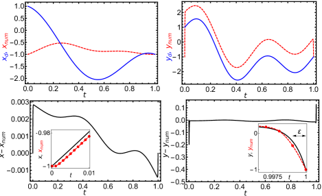
Figure 1: Optimal trajectory tracking for the damped mathematical pendulum. Top: While the numerically obtained, optimally controlled angular velocity $y_{num}$ (red dashed) resembles the desired velocity $y_{d}$ (blue solid) in shape (right), the angular displacement $x_{num}$ (left) is far off its desired counterpart $x_{d}$. Bottom: The difference between analytical and numerical solution for the optimally controlled state reveals excellent agreement except close to the time domain boundaries. To leading order in the small parameter $\varepsilon$, the analytical results predicts a boundary layer of width $\varepsilon$ for $y$ (right inset) but not for $x$ (left inset). As indicated by the red dots, the temporal resolution $\Delta t=\varepsilon=10^{-3}$ is just large enough to resolve the boundary layer.

Results for a two-dimensional dynamical system.

We compare the approximate analytical solution for small but finite $\varepsilon>0$ with numerical results for the optimally controlled damped mathematical pendulum. The model is of the form Eq. (1) which satisfies the linearizing assumption. The EOM are

$$\dot{x} =y, \dot{y} =-\frac{1}{2}y-\sin\left(x\right)+\left(1+\frac{1}{4}x^{2}\right)u,$$ (34)

with $x$ denoting the angular displacement and $y$ the angular velocity. The desired trajectory $\boldsymbol{x}_{d}=\left(x_{d},y_{d}\right)^{T}$ is $x_{d}\left(t\right)=\cos\left(2\pi t\right)-2t$, $y_{d}\left(t\right)=x_{d}\left(t\right)+\sin\left(4\pi t\right)$. The terminal conditions $x\left(1\right)=x_{d}\left(1\right)=-1$ and $y\left(1\right)=y_{d}\left(1\right)=-1$ are chosen to lie on the desired trajectory, while the initial conditions $x\left(0\right)=-1$ and $y\left(0\right)=-1$ do not. Explicit analytical expressions for the optimally controlled composite state solution and the optimal control signal can be found in the SM sup . The prescribed desired trajectory is not exactly realizable, which can be understood from physical reasoning. A point mass governed by Newton’s EOM can only trace out desired trajectories in phase space, spanned by $x$ and $y$, which satisfy $\dot{x}_{d}=y_{d}$. This relation simply defines the velocity, and no control force of whatever amplitude can change that definition Löber (2016). Numerical computations are performed with the ACADO Toolkit Houska et al. (2011), an open source program package for solving optimal control problems. The problem is solved on a time interval of length $1$ with a time step width $\Delta t=10^{-3}$. A straightforward numerical solution of the necessary optimality conditions Eqs. (4)-(6) is usually impossible due to the mixed boundary conditions. While half of the $2n$ boundary conditions are imposed at the initial time, the other half are imposed at the terminal time. This typically requires iterative algorithms such as shooting, and renders optimal trajectory tracking computationally expensive.
Figure 1 top compares the desired trajectory $\boldsymbol{x}_{d}$ for angular displacement $x$ (left) and velocity $y$ (right) with the numerically computed, optimally controlled state $\boldsymbol{x}$. While the controlled velocity looks similar in shape to the desired trajectory, the controlled displacement is way off. Even though the terminal conditions comply with the desired trajectory, the solution for $y$ exhibits some very steep transients at both ends of the time interval. These transitions are the boundary layers of width $\varepsilon=10^{-3}$ described by the inner solutions. On this scale, there is no visible difference between the analytically and numerically obtained controlled state. We plot the difference between them in Fig. 1 bottom. Apart from the boundary layer region, the agreement is excellent. Deviations in the boundary layer region can be understood from the relatively poor numerical resolution equal to the boundary layer width, $\Delta t=\varepsilon$, see the insets for closeups of the boundary layers regions. Increasing $\Delta t$ leads to larger numerical errors but decreasing $\Delta t$ quickly increases computation time. While the analytical leading order result predicts a boundary layer for $y$ but not for $x$, the numerical solution for $x$ exhibits a tiny boundary layer, which we expect analytically to arise from higher order contributions in the perturbation expansion.

Exact solution for $\varepsilon=0$.

For $\varepsilon=0$, the inner solutions do not play a role because the boundary layers exhibited by $\boldsymbol{\mathcal{P}}\boldsymbol{x}$ degenerate to jumps,

$$\boldsymbol{\mathcal{P}}\boldsymbol{x} =\begin{cases}\boldsymbol{\mathcal{P}}\boldsymbol{x}_{0},&t=t_{0},\\ \boldsymbol{\mathcal{P}}\boldsymbol{x}_{d}-\boldsymbol{\Omega}\boldsymbol{\mathcal{A}}^{T}\boldsymbol{\mathcal{Q}}^{T}\boldsymbol{\Lambda},&t_{0}<t<t_{1},\\ \boldsymbol{\mathcal{P}}\boldsymbol{x}_{1},&t=t_{1}.\end{cases}$$ (35)

The jump heights are fully determined by the outer solution $\boldsymbol{\mathcal{Q}}^{T}\boldsymbol{\Lambda}$ and the boundary conditions. The parts $\boldsymbol{\mathcal{P}}^{T}\boldsymbol{\lambda}=\boldsymbol{\mathcal{P}}^{T}\boldsymbol{\Lambda}=\boldsymbol{0}$ vanish identically for all times. The parts $\boldsymbol{\mathcal{Q}}^{T}\boldsymbol{\lambda}=\boldsymbol{\mathcal{Q}}^{T}\boldsymbol{\Lambda}$ and $\boldsymbol{\mathcal{Q}}\boldsymbol{x}=\boldsymbol{\mathcal{Q}}\boldsymbol{X}$ are from the linear outer equations (27). Cast in terms of the state transition matrix $\boldsymbol{\Phi}\left(t,t_{0}\right)=\exp\left(\boldsymbol{\mathcal{M}}\left(t-t_{0}\right)\right)$, the solutions become

$$\left(\begin{array}[]{c}\boldsymbol{\mathcal{Q}}^{T}\boldsymbol{\Lambda}\left(t\right)\\ \boldsymbol{\mathcal{Q}}\boldsymbol{X}\left(t\right)\end{array}\right) =\boldsymbol{\Phi}\left(t,t_{0}\right)\left(\begin{array}[]{c}\boldsymbol{\mathcal{Q}}^{T}\boldsymbol{\Lambda}_{\text{init}}\\ \boldsymbol{\mathcal{Q}}\boldsymbol{x}_{0}\end{array}\right)$$ (40)

$$+\int_{t_{0}}^{t}d\tau\boldsymbol{\Phi}\left(t,\tau\right)\left(\begin{array}[]{c}\boldsymbol{\mathcal{Q}}^{T}\boldsymbol{\mathcal{S}}\boldsymbol{\mathcal{Q}}\boldsymbol{x}_{d}\left(\tau\right)\\ \boldsymbol{\mathcal{Q}}\boldsymbol{\mathcal{A}}\boldsymbol{\mathcal{P}}\boldsymbol{x}_{d}\left(\tau\right)+\boldsymbol{\mathcal{Q}}\boldsymbol{b}\end{array}\right).$$ (43)

The parameter $\boldsymbol{\mathcal{Q}}^{T}\boldsymbol{\Lambda}_{\text{init}}$ is determined from the terminal condition $\boldsymbol{\mathcal{Q}}\boldsymbol{x}\left(t_{1}\right)=\boldsymbol{\mathcal{Q}}\boldsymbol{x}_{1}$. The control is given in terms of $\boldsymbol{x}$ by Eq. (10). We obtain (see the SM sup for a derivation),

$$\boldsymbol{u} =\begin{cases}\boldsymbol{u}_{0},&t=t_{0},\\ \boldsymbol{\mathcal{B}}^{g}\left(\boldsymbol{X}\right)\left(\boldsymbol{\dot{X}}-\boldsymbol{R}\left(\boldsymbol{X}\right)\right),&t_{0}<t<t_{1},\\ \boldsymbol{u}_{1},&t=t_{1},\end{cases}$$ (44)

with

$$\boldsymbol{u}_{i} =\boldsymbol{\mathcal{B}}^{g}\left(\boldsymbol{x}_{i}\right)\left(\boldsymbol{\dot{X}}\left(t_{i}\right)-\boldsymbol{R}\left(\boldsymbol{x}_{i}\right)\right)$$

$$+\left(-1\right)^{i}2\boldsymbol{\mathcal{B}}^{g}\left(\boldsymbol{x}_{i}\right)\left(\boldsymbol{X}\left(t_{i}\right)-\boldsymbol{x}_{i}\right)\delta\left(t-t_{i}\right).$$ (45)

Because of $\boldsymbol{u}\sim\boldsymbol{\mathcal{P}}\boldsymbol{\dot{x}}$, the jumps of $\boldsymbol{\mathcal{P}}\boldsymbol{x}$ at the time domain boundaries lead to divergences $\delta\left(t\right)$ in form of Dirac delta functions located at the time domain boundaries.

Conclusions.

For $\varepsilon>0$, the dynamics of an optimal control system takes place in the in the combined state space of state $\boldsymbol{x}$ and co-state $\boldsymbol{\lambda}$ of dimension $2n$. For $\varepsilon=0$, the dynamics is restricted by $2p$ algebraic equations, $\boldsymbol{\mathcal{P}}^{T}\boldsymbol{\lambda}=\boldsymbol{0}$ and Eq. (35), to a hypersurface of dimension $2\left(n-p\right)$, also called a singular surface Bryson and Ho (1975). At the initial and terminal time, kicks in form of a Dirac delta function mediated by control induce an instantaneous transition from $\boldsymbol{x}_{0}$ onto the singular surface and from the singular surface to $\boldsymbol{x}_{1}$, respectively. These instantaneous transitions render the state components $\boldsymbol{\mathcal{P}}\boldsymbol{x}$ discontinuous at the initial and terminal time, respectively. For $\varepsilon>0$, the discontinuities are smoothed out in form of boundary layers, i.e., continuous transition regions with a slope and width controlled by $\varepsilon$. The control signals are finite and exhibit a sharp peak at the time domain boundaries, with an amplitude inversely proportional to $\varepsilon$. This general picture of optimal trajectory tracking for small $\varepsilon$ is independent of the linearizing assumption and remains true for arbitrary affine control systems Löber (2015).

In experiments and numerical simulations, it is impossible to generate diverging control signals. In practice, a finite value $\varepsilon>0$ in Eq. (2) is indispensable. Nevertheless, understanding the behavior of control systems in the limit $\varepsilon\rightarrow 0$ is very useful for applications. For example, to prevent or at least minimize any steep transitions and large control amplitudes, we may choose the initial state to lie on the singular surface. Furthermore, a faithful numerical representation of the solution to optimal control requires a temporal resolution $\Delta t\lesssim\varepsilon$ to resolve the initial and terminal boundary layers.

The linearizing assumption yields linear algebraic and differential outer equations. While the inner equations may still be nonlinear for $\varepsilon>0$, they reduce to jumps, with jump heights independent of any details of the inner equations. Consequently, for $\varepsilon=0$, the exact solution for $\boldsymbol{x}$, $\boldsymbol{\lambda}$, and $\boldsymbol{u}$, is entirely given in terms of the linear outer equations. For models of the form Eq. (1), this culminates in the following, surprising conclusion. The controlled state becomes independent of the external force $R$ as $\varepsilon=0$. Furthermore, the dependence on the nonlinearity $b$ is restricted to the boundary layers, which become irrelevant for $\varepsilon=0$. Consequently, for a given desired trajectory $\boldsymbol{x}_{d}$, and given initial and terminal conditions, and $\varepsilon=0$, all optimally controlled states of Eq. (1) trace out the same trajectories in phase space, independent of $R$ and $b$. However, note that the control signal $u$ still depends on $R$ and $b$.

Intuitively, the result can be understood as follows. The state components which and which are not acted upon directly by control are encoded in the matrices $\boldsymbol{\mathcal{P}}$ and $\boldsymbol{\mathcal{Q}}$, respectively. Assumption (19) of the linearizing assumption demands that the control acts on the nonlinear state equations, and all other equations are linear. For $\varepsilon=0$, the control amplitude is unrestricted. The control dominates over the nonlinearity and can absorb an arbitrarily large part $\boldsymbol{\mathcal{P}}\boldsymbol{R}$ of $\boldsymbol{R}$, resulting in linear evolution equations. The linearizing assumption is satisfied by all models of the form $\dot{x}=a_{0}+a_{1}y+a_{2}x,\,\dot{y}=R\left(x,y\right)+b\left(x,y\right)u$, which includes Eq. (1) and the FitzHugh-Nagumo model with a control acting on the activator $y$ as special cases. Another example is the SIR model for disease transmission with the transmission rate serving as the control Löber (2015).

Generalizations of the results presented here are possible. One example are noisy controlled systems, for which fundamental results exist for linear optimal control in form of the linear-quadratic regulator Bryson and Ho (1975). In this context, we mention Ref. Kappen (2005) which presents a linear theory for the control of nonlinear stochastic systems. However, the method in Kappen (2005) is restricted to systems with identical numbers of control signals and state components, $n=p$. Other possibilities are generalizations to spatio-temporal systems as e.g. reaction-diffusion systems Löber and Engel (2014).

Supplemental Material: Linear structures in nonlinear optimal trajectory tracking

Jakob Löber*

Institut für Theoretische Physik, EW 7-1, Hardenbergstraße 36, Technische Universität Berlin, 10623 Berlin

Appendix A: Rearranging the necessary optimality conditions

Here, we give a detailed version of the rearrangement of the necessary optimality conditions,

$$\boldsymbol{0} =\varepsilon^{2}\boldsymbol{u}\left(t\right)+\boldsymbol{\mathcal{B}}^{T}\left(\boldsymbol{x}\left(t\right)\right)\boldsymbol{\lambda}\left(t\right),$$ (S1)

$$\boldsymbol{\dot{x}}\left(t\right) =\boldsymbol{R}\left(\boldsymbol{x}\left(t\right)\right)+\boldsymbol{\mathcal{B}}\left(\boldsymbol{x}\left(t\right)\right)\boldsymbol{u}\left(t\right),$$ (S2)

$$-\boldsymbol{\dot{\lambda}}\left(t\right) =\left(\nabla\boldsymbol{R}^{T}\left(\boldsymbol{x}\left(t\right)\right)+\left(\nabla\boldsymbol{\mathcal{B}}\left(\boldsymbol{x}\left(t\right)\right)\boldsymbol{u}\left(t\right)\right)^{T}\right)\boldsymbol{\lambda}\left(t\right)+\boldsymbol{\mathcal{S}}\left(\boldsymbol{x}\left(t\right)-\boldsymbol{x}_{d}\left(t\right)\right),$$ (S3)

with the initial and terminal conditions

$$\boldsymbol{x}\left(t_{0}\right) =\boldsymbol{x}_{0}, \boldsymbol{x}\left(t_{1}\right) =\boldsymbol{x}_{1}.$$ (S4)

Together with the assumption $0\leq\varepsilon\ll 1$, the rearrangement will enable the reinterpretation of Eqs. (S1)-(S3) as a singularly perturbed system of differential equations. To shorten the notation, the time argument of $\boldsymbol{x}=\boldsymbol{x}\left(t\right)$, $\boldsymbol{\lambda}=\boldsymbol{\lambda}\left(t\right)$ and $\boldsymbol{u}=\boldsymbol{u}\left(t\right)$ is suppressed in the following and some abbreviating matrices are introduced. Let the $n\times n$ matrix $\boldsymbol{\Omega}\left(\boldsymbol{x}\right)$ be defined by

$$\boldsymbol{\Omega}\left(\boldsymbol{x}\right) =\boldsymbol{\mathcal{B}}\left(\boldsymbol{x}\right)\left(\boldsymbol{\mathcal{B}}^{T}\left(\boldsymbol{x}\right)\boldsymbol{\mathcal{S}}\boldsymbol{\mathcal{B}}\left(\boldsymbol{x}\right)\right)^{-1}\boldsymbol{\mathcal{B}}^{T}\left(\boldsymbol{x}\right).$$ (S5)

A simple calculation shows that $\boldsymbol{\Omega}\left(\boldsymbol{x}\right)$ is symmetric,

$$\boldsymbol{\Omega}^{T}\left(\boldsymbol{x}\right) =\boldsymbol{\mathcal{B}}\left(\boldsymbol{x}\right)\left(\boldsymbol{\mathcal{B}}^{T}\left(\boldsymbol{x}\right)\boldsymbol{\mathcal{S}}\boldsymbol{\mathcal{B}}\left(\boldsymbol{x}\right)\right)^{-T}\boldsymbol{\mathcal{B}}^{T}\left(\boldsymbol{x}\right)=\boldsymbol{\mathcal{B}}\left(\boldsymbol{x}\right)\left(\boldsymbol{\mathcal{B}}^{T}\left(\boldsymbol{x}\right)\boldsymbol{\mathcal{S}}\boldsymbol{\mathcal{B}}\left(\boldsymbol{x}\right)\right)^{-1}\boldsymbol{\mathcal{B}}^{T}\left(\boldsymbol{x}\right)=\boldsymbol{\Omega}\left(\boldsymbol{x}\right).$$ (S6)

Note that $\boldsymbol{\mathcal{B}}^{T}\left(\boldsymbol{x}\right)\boldsymbol{\mathcal{S}}\boldsymbol{\mathcal{B}}\left(\boldsymbol{x}\right)=\left(\boldsymbol{\mathcal{B}}^{T}\left(\boldsymbol{x}\right)\boldsymbol{\mathcal{S}}\boldsymbol{\mathcal{B}}\left(\boldsymbol{x}\right)\right)^{T}$ is a symmetric $p\times p$ matrix because $\boldsymbol{\mathcal{S}}$ is symmetric by assumption, and the inverse of a symmetric matrix is symmetric. Let the two $n\times n$ projection matrices $\boldsymbol{\mathcal{P}}\left(\boldsymbol{x}\right)$ and $\boldsymbol{\mathcal{Q}}\left(\boldsymbol{x}\right)$ be defined by

$$\boldsymbol{\mathcal{P}}\left(\boldsymbol{x}\right) =\boldsymbol{\Omega}\left(\boldsymbol{x}\right)\boldsymbol{\mathcal{S}}, \boldsymbol{\mathcal{Q}}\left(\boldsymbol{x}\right) =\mathbf{1}-\boldsymbol{\mathcal{P}}\left(\boldsymbol{x}\right).$$ (S7)

$\boldsymbol{\mathcal{P}}\left(\boldsymbol{x}\right)$ and $\boldsymbol{\mathcal{Q}}\left(\boldsymbol{x}\right)$ are idempotent, $\boldsymbol{\mathcal{P}}^{2}\left(\boldsymbol{x}\right)=\boldsymbol{\mathcal{P}}\left(\boldsymbol{x}\right)$ and $\boldsymbol{\mathcal{Q}}^{2}\left(\boldsymbol{x}\right)=\boldsymbol{\mathcal{Q}}\left(\boldsymbol{x}\right)$. Furthermore, $\boldsymbol{\mathcal{P}}\left(\boldsymbol{x}\right)$ and $\boldsymbol{\mathcal{Q}}\left(\boldsymbol{x}\right)$ satisfy the relations

$$\boldsymbol{\mathcal{P}}\left(\boldsymbol{x}\right)\boldsymbol{\mathcal{B}}\left(\boldsymbol{x}\right) =\boldsymbol{\mathcal{B}}\left(\boldsymbol{x}\right), \boldsymbol{\mathcal{Q}}\left(\boldsymbol{x}\right)\boldsymbol{\mathcal{B}}\left(\boldsymbol{x}\right) =\boldsymbol{0}, \boldsymbol{\mathcal{B}}^{T}\left(\boldsymbol{x}\right)\boldsymbol{\mathcal{S}}\boldsymbol{\mathcal{P}}\left(\boldsymbol{x}\right) =\boldsymbol{\mathcal{B}}^{T}\left(\boldsymbol{x}\right)\boldsymbol{\mathcal{S}}, \boldsymbol{\mathcal{B}}^{T}\left(\boldsymbol{x}\right)\boldsymbol{\mathcal{S}}\boldsymbol{\mathcal{Q}} =\boldsymbol{0}.$$ (S8)

Computing the transposed of $\boldsymbol{\mathcal{P}}\left(\boldsymbol{x}\right)$ and $\boldsymbol{\mathcal{Q}}\left(\boldsymbol{x}\right)$ yields

$$\boldsymbol{\mathcal{P}}^{T}\left(\boldsymbol{x}\right) =\boldsymbol{\mathcal{S}}^{T}\boldsymbol{\Omega}^{T}\left(\boldsymbol{x}\right)=\boldsymbol{\mathcal{S}}\boldsymbol{\Omega}\left(\boldsymbol{x}\right)\neq\boldsymbol{\mathcal{P}}\left(\boldsymbol{x}\right),$$ (S9)

and analogously for $\boldsymbol{\mathcal{Q}}\left(\boldsymbol{x}\right)$. Equation (S9) shows that $\boldsymbol{\mathcal{P}}\left(\boldsymbol{x}\right)$, and therefore also $\boldsymbol{\mathcal{Q}}\left(\boldsymbol{x}\right)$, is not symmetric. However, $\boldsymbol{\mathcal{P}}^{T}\left(\boldsymbol{x}\right)$ satisfies the convenient property

$$\boldsymbol{\mathcal{P}}^{T}\left(\boldsymbol{x}\right)\boldsymbol{\mathcal{S}} =\boldsymbol{\mathcal{S}}\boldsymbol{\Omega}\left(\boldsymbol{x}\right)\boldsymbol{\mathcal{S}}=\boldsymbol{\mathcal{S}}\boldsymbol{\mathcal{P}}\left(\boldsymbol{x}\right),$$ (S10)

which implies

$$\boldsymbol{\mathcal{P}}^{T}\left(\boldsymbol{x}\right)\boldsymbol{\mathcal{S}} =\boldsymbol{\mathcal{P}}^{T}\left(\boldsymbol{x}\right)\boldsymbol{\mathcal{P}}^{T}\left(\boldsymbol{x}\right)\boldsymbol{\mathcal{S}}=\boldsymbol{\mathcal{P}}^{T}\left(\boldsymbol{x}\right)\boldsymbol{\mathcal{S}}\boldsymbol{\mathcal{P}}\left(\boldsymbol{x}\right),$$ (S11)

and similarly for $\boldsymbol{\mathcal{S}}\boldsymbol{\mathcal{Q}}\left(\boldsymbol{x}\right)$. The product of $\boldsymbol{\Omega}\left(\boldsymbol{x}\right)$ with $\boldsymbol{\mathcal{P}}^{T}\left(\boldsymbol{x}\right)$ yields

$$\boldsymbol{\Omega}\left(\boldsymbol{x}\right)\boldsymbol{\mathcal{P}}^{T}\left(\boldsymbol{x}\right) =\boldsymbol{\Omega}\left(\boldsymbol{x}\right)\boldsymbol{\mathcal{S}}\boldsymbol{\Omega}\left(\boldsymbol{x}\right)=\boldsymbol{\mathcal{B}}\left(\boldsymbol{x}\right)\left(\boldsymbol{\mathcal{B}}^{T}\left(\boldsymbol{x}\right)\boldsymbol{\mathcal{S}}\boldsymbol{\mathcal{B}}\left(\boldsymbol{x}\right)\right)^{-1}\boldsymbol{\mathcal{B}}^{T}\left(\boldsymbol{x}\right)=\boldsymbol{\Omega}\left(\boldsymbol{x}\right),$$ (S12)

and

$$\boldsymbol{\Omega}\left(\boldsymbol{x}\right)\boldsymbol{\mathcal{P}}^{T}\left(\boldsymbol{x}\right)\boldsymbol{\mathcal{S}} =\boldsymbol{\Omega}\left(\boldsymbol{x}\right)\boldsymbol{\mathcal{S}}=\boldsymbol{\mathcal{P}}\left(\boldsymbol{x}\right).$$ (S13)

Let the $n\times n$ matrix $\boldsymbol{\Gamma}\left(\boldsymbol{x}\right)$ be defined by

$$\boldsymbol{\Gamma}\left(\boldsymbol{x}\right) =\boldsymbol{\mathcal{S}}\boldsymbol{\mathcal{B}}\left(\boldsymbol{x}\right)\left(\boldsymbol{\mathcal{B}}^{T}\left(\boldsymbol{x}\right)\boldsymbol{\mathcal{S}}\boldsymbol{\mathcal{B}}\left(\boldsymbol{x}\right)\right)^{-2}\boldsymbol{\mathcal{B}}^{T}\left(\boldsymbol{x}\right)\boldsymbol{\mathcal{S}}.$$ (S14)

$\boldsymbol{\Gamma}\left(\boldsymbol{x}\right)$ is symmetric,

$$\boldsymbol{\Gamma}^{T}\left(\boldsymbol{x}\right) =\left(\boldsymbol{\mathcal{S}}\boldsymbol{\mathcal{B}}\left(\boldsymbol{x}\right)\left(\boldsymbol{\mathcal{B}}^{T}\left(\boldsymbol{x}\right)\boldsymbol{\mathcal{S}}\boldsymbol{\mathcal{B}}\left(\boldsymbol{x}\right)\right)^{-2}\boldsymbol{\mathcal{B}}^{T}\left(\boldsymbol{x}\right)\boldsymbol{\mathcal{S}}\right)^{T}=\boldsymbol{\mathcal{S}}\boldsymbol{\mathcal{B}}\left(\boldsymbol{x}\right)\left(\boldsymbol{\mathcal{B}}^{T}\left(\boldsymbol{x}\right)\boldsymbol{\mathcal{S}}\boldsymbol{\mathcal{B}}\left(\boldsymbol{x}\right)\right)^{-2T}\boldsymbol{\mathcal{B}}^{T}\left(\boldsymbol{x}\right)\boldsymbol{\mathcal{S}}=\boldsymbol{\Gamma}\left(\boldsymbol{x}\right),$$ (S15)

and satisfies

$$\boldsymbol{\Gamma}\left(\boldsymbol{x}\right)\boldsymbol{\mathcal{P}}\left(\boldsymbol{x}\right)= \boldsymbol{\mathcal{S}}\boldsymbol{\mathcal{B}}\left(\boldsymbol{x}\right)\left(\boldsymbol{\mathcal{B}}^{T}\left(\boldsymbol{x}\right)\boldsymbol{\mathcal{S}}\boldsymbol{\mathcal{B}}\left(\boldsymbol{x}\right)\right)^{-2}\boldsymbol{\mathcal{B}}^{T}\left(\boldsymbol{x}\right)\boldsymbol{\mathcal{S}}\boldsymbol{\mathcal{B}}\left(\boldsymbol{x}\right)\left(\boldsymbol{\mathcal{B}}^{T}\left(\boldsymbol{x}\right)\boldsymbol{\mathcal{S}}\boldsymbol{\mathcal{B}}\left(\boldsymbol{x}\right)\right)^{-1}\boldsymbol{\mathcal{B}}^{T}\left(\boldsymbol{x}\right)\boldsymbol{\mathcal{S}}$$

$$= \boldsymbol{\mathcal{S}}\boldsymbol{\mathcal{B}}\left(\boldsymbol{x}\right)\left(\boldsymbol{\mathcal{B}}^{T}\left(\boldsymbol{x}\right)\boldsymbol{\mathcal{S}}\boldsymbol{\mathcal{B}}\left(\boldsymbol{x}\right)\right)^{-2}\boldsymbol{\mathcal{B}}^{T}\left(\boldsymbol{x}\right)\boldsymbol{\mathcal{S}}=\boldsymbol{\Gamma}\left(\boldsymbol{x}\right).$$ (S16)

Transposing yields

$$\left(\boldsymbol{\Gamma}\left(\boldsymbol{x}\right)\boldsymbol{\mathcal{P}}\left(\boldsymbol{x}\right)\right)^{T} =\boldsymbol{\mathcal{P}}^{T}\left(\boldsymbol{x}\right)\boldsymbol{\Gamma}^{T}\left(\boldsymbol{x}\right)=\boldsymbol{\mathcal{P}}^{T}\left(\boldsymbol{x}\right)\boldsymbol{\Gamma}\left(\boldsymbol{x}\right)=\boldsymbol{\Gamma}\left(\boldsymbol{x}\right).$$ (S17)

The projectors $\boldsymbol{\mathcal{P}}\left(\boldsymbol{x}\right)$ and $\boldsymbol{\mathcal{Q}}\left(\boldsymbol{x}\right)$ are used to partition the state $\boldsymbol{x}$ as

$$\boldsymbol{x} =\boldsymbol{\mathcal{P}}\left(\boldsymbol{x}\right)\boldsymbol{x}+\boldsymbol{\mathcal{Q}}\left(\boldsymbol{x}\right)\boldsymbol{x}.$$ (S18)

The controlled state equation (S2) is split in two parts by multiplying with $\boldsymbol{\mathcal{P}}\left(\boldsymbol{x}\right)$ and with $\boldsymbol{\mathcal{Q}}\left(\boldsymbol{x}\right)$ from the left,

$$\boldsymbol{\mathcal{P}}\left(\boldsymbol{x}\right)\boldsymbol{\dot{x}} =\boldsymbol{\mathcal{P}}\left(\boldsymbol{x}\right)\boldsymbol{R}\left(\boldsymbol{x}\right)+\boldsymbol{\mathcal{B}}\left(\boldsymbol{x}\right)\boldsymbol{u}, \boldsymbol{\mathcal{Q}}\left(\boldsymbol{x}\right)\boldsymbol{\dot{x}} =\boldsymbol{\mathcal{Q}}\left(\boldsymbol{x}\right)\boldsymbol{R}\left(\boldsymbol{x}\right).$$ (S19)

The initial and terminal conditions are split up as well,

$$\boldsymbol{\mathcal{P}}\left(\boldsymbol{x}\left(t_{0}\right)\right)\boldsymbol{x}\left(t_{0}\right) =\boldsymbol{\mathcal{P}}\left(\boldsymbol{x}_{0}\right)\boldsymbol{x}_{0}, \boldsymbol{\mathcal{Q}}\left(\boldsymbol{x}\left(t_{0}\right)\right)\boldsymbol{x}\left(t_{0}\right) =\boldsymbol{\mathcal{Q}}\left(\boldsymbol{x}_{0}\right)\boldsymbol{x}_{0},$$ (S20)

$$\boldsymbol{\mathcal{P}}\left(\boldsymbol{x}\left(t_{1}\right)\right)\boldsymbol{x}\left(t_{1}\right) =\boldsymbol{\mathcal{P}}\left(\boldsymbol{x}_{1}\right)\boldsymbol{x}_{1}, \boldsymbol{\mathcal{Q}}\left(\boldsymbol{x}\left(t_{1}\right)\right)\boldsymbol{x}\left(t_{1}\right) =\boldsymbol{\mathcal{Q}}\left(\boldsymbol{x}_{1}\right)\boldsymbol{x}_{1}.$$ (S21)

Multiplying the first equation of Eq. (S19) by $\boldsymbol{\mathcal{B}}^{T}\left(\boldsymbol{x}\right)\boldsymbol{\mathcal{S}}$ from the left and using $\boldsymbol{\mathcal{B}}^{T}\left(\boldsymbol{x}\right)\boldsymbol{\mathcal{S}}\boldsymbol{\mathcal{P}}\left(\boldsymbol{x}\right)=\boldsymbol{\mathcal{B}}^{T}\left(\boldsymbol{x}\right)\boldsymbol{\mathcal{S}}$ yields an expression for the control $\boldsymbol{u}$ in terms of the controlled state trajectory $\boldsymbol{x}$,

$$\boldsymbol{u} =\left(\boldsymbol{\mathcal{B}}^{T}\left(\boldsymbol{x}\right)\boldsymbol{\mathcal{S}}\boldsymbol{\mathcal{B}}\left(\boldsymbol{x}\right)\right)^{-1}\boldsymbol{\mathcal{B}}^{T}\left(\boldsymbol{x}\right)\boldsymbol{\mathcal{S}}\left(\boldsymbol{\dot{x}}-\boldsymbol{R}\left(\boldsymbol{x}\right)\right)=\boldsymbol{\mathcal{B}}^{g}\left(\boldsymbol{x}\right)\left(\boldsymbol{\dot{x}}-\boldsymbol{R}\left(\boldsymbol{x}\right)\right).$$ (S22)

The $p\times n$ matrix $\boldsymbol{\mathcal{B}}^{g}\left(\boldsymbol{x}\right)$ is defined by

$$\boldsymbol{\mathcal{B}}^{g}\left(\boldsymbol{x}\right) =\left(\boldsymbol{\mathcal{B}}^{T}\left(\boldsymbol{x}\right)\boldsymbol{\mathcal{S}}\boldsymbol{\mathcal{B}}\left(\boldsymbol{x}\right)\right)^{-1}\boldsymbol{\mathcal{B}}^{T}\left(\boldsymbol{x}\right)\boldsymbol{\mathcal{S}}.$$ (S23)

The matrix $\boldsymbol{\mathcal{B}}^{g}\left(\boldsymbol{x}\right)$ can be used to rewrite the matrices $\boldsymbol{\mathcal{P}}\left(\boldsymbol{x}\right)$ and $\boldsymbol{\Gamma}\left(\boldsymbol{x}\right)$ as

$$\boldsymbol{\mathcal{P}}\left(\boldsymbol{x}\right) =\boldsymbol{\mathcal{B}}\left(\boldsymbol{x}\right)\boldsymbol{\mathcal{B}}^{g}\left(\boldsymbol{x}\right), \boldsymbol{\Gamma}\left(\boldsymbol{x}\right) =\boldsymbol{\mathcal{B}}^{gT}\left(\boldsymbol{x}\right)\boldsymbol{\mathcal{B}}^{g}\left(\boldsymbol{x}\right),$$ (S24)

respectively.
The solution for $\boldsymbol{u}$ is inserted in the stationarity condition Eq. (S1) to yield

$$\boldsymbol{0} =\varepsilon^{2}\boldsymbol{u}^{T}+\boldsymbol{\lambda}^{T}\boldsymbol{\mathcal{B}}\left(\boldsymbol{x}\right)=\varepsilon^{2}\left(\boldsymbol{\dot{x}}^{T}-\boldsymbol{R}^{T}\left(\boldsymbol{x}\right)\right)\boldsymbol{\mathcal{B}}^{gT}\left(\boldsymbol{x}\right)+\boldsymbol{\lambda}^{T}\boldsymbol{\mathcal{B}}\left(\boldsymbol{x}\right).$$ (S25)

Equation (S25) is utilized to eliminate any occurrence of the part $\boldsymbol{\mathcal{P}}^{T}\left(\boldsymbol{x}\right)\boldsymbol{\lambda}$ in all equations. In contrast to the state $\boldsymbol{x}$, cf. Eq. (S18), the co-state is split up with the transposed projectors $\boldsymbol{\mathcal{P}}^{T}\left(\boldsymbol{x}\right)$ and $\boldsymbol{\mathcal{Q}}^{T}\left(\boldsymbol{x}\right)$,

$$\boldsymbol{\lambda} =\boldsymbol{\mathcal{P}}^{T}\left(\boldsymbol{x}\right)\boldsymbol{\lambda}+\boldsymbol{\mathcal{Q}}^{T}\left(\boldsymbol{x}\right)\boldsymbol{\lambda}.$$ (S26)

Multiplying Eq. (S25) with $\boldsymbol{\mathcal{B}}^{g}\left(\boldsymbol{x}\right)$ from the right and using Eq. (S24) yields an expression for $\boldsymbol{\mathcal{P}}^{T}\left(\boldsymbol{x}\right)\boldsymbol{\lambda}$,

$$\boldsymbol{0} =\varepsilon^{2}\left(\boldsymbol{\dot{x}}^{T}-\boldsymbol{R}^{T}\left(\boldsymbol{x}\right)\right)\boldsymbol{\Gamma}\left(\boldsymbol{x}\right)+\boldsymbol{\lambda}^{T}\boldsymbol{\mathcal{P}}\left(\boldsymbol{x}\right).$$ (S27)

Transposing the last equation and exploiting the symmetry of $\boldsymbol{\Gamma}\left(\boldsymbol{x}\right)$, Eq. (S15), yields

$$\boldsymbol{\mathcal{P}}^{T}\left(\boldsymbol{x}\right)\boldsymbol{\lambda} =-\varepsilon^{2}\boldsymbol{\Gamma}\left(\boldsymbol{x}\right)\left(\boldsymbol{\dot{x}}-\boldsymbol{R}\left(\boldsymbol{x}\right)\right).$$ (S28)

Equation (S28) is valid for all times $t_{0}\leq t\leq t_{1}$ such that we can apply the time derivative to get

$$\boldsymbol{0} =\varepsilon^{2}\boldsymbol{\Gamma}\left(\boldsymbol{x}\right)\left(\boldsymbol{\ddot{x}}-\nabla\boldsymbol{R}\left(\boldsymbol{x}\right)\boldsymbol{\dot{x}}\right)+\varepsilon^{2}\boldsymbol{\dot{\Gamma}}\left(\boldsymbol{x}\right)\left(\boldsymbol{\dot{x}}-\boldsymbol{R}\left(\boldsymbol{x}\right)\right)+\boldsymbol{\mathcal{\dot{P}}}^{T}\left(\boldsymbol{x}\right)\boldsymbol{\lambda}+\boldsymbol{\mathcal{P}}^{T}\left(\boldsymbol{x}\right)\boldsymbol{\dot{\lambda}}.$$ (S29)

The short hand notations

$$\boldsymbol{\dot{\Gamma}}\left(\boldsymbol{x}\right) =\dfrac{d}{dt}\boldsymbol{\Gamma}\left(\boldsymbol{x}\right)=\sum_{j=1}^{n}\dfrac{\partial}{\partial x_{j}}\boldsymbol{\Gamma}\left(\boldsymbol{x}\right)\dot{x}_{j}, \boldsymbol{\mathcal{\dot{P}}}^{T}\left(\boldsymbol{x}\right) =\dfrac{d}{dt}\boldsymbol{\mathcal{P}}^{T}\left(\boldsymbol{x}\right)=\sum_{j=1}^{n}\dfrac{\partial}{\partial x_{j}}\boldsymbol{\mathcal{P}}^{T}\left(\boldsymbol{x}\right)\dot{x}_{j},$$ (S30)

were introduced in Eq. (S29). Splitting the co-state $\boldsymbol{\lambda}$ as in Eq. (S26) and using Eq. (S28) to eliminate $\boldsymbol{\mathcal{P}}^{T}\left(\boldsymbol{x}\right)\boldsymbol{\lambda}$ leads to

$$-\boldsymbol{\mathcal{P}}^{T}\left(\boldsymbol{x}\right)\boldsymbol{\dot{\lambda}} =\varepsilon^{2}\boldsymbol{\Gamma}\left(\boldsymbol{x}\right)\left(\boldsymbol{\ddot{x}}-\nabla\boldsymbol{R}\left(\boldsymbol{x}\right)\boldsymbol{\dot{x}}\right)+\boldsymbol{\mathcal{\dot{P}}}^{T}\left(\boldsymbol{x}\right)\boldsymbol{\mathcal{Q}}^{T}\left(\boldsymbol{x}\right)\boldsymbol{\lambda}+\varepsilon^{2}\left(\boldsymbol{\dot{\Gamma}}\left(\boldsymbol{x}\right)-\boldsymbol{\mathcal{\dot{P}}}^{T}\left(\boldsymbol{x}\right)\boldsymbol{\Gamma}\left(\boldsymbol{x}\right)\right)\left(\boldsymbol{\dot{x}}-\boldsymbol{R}\left(\boldsymbol{x}\right)\right).$$ (S31)

Equation (S31) is an expression for $\boldsymbol{\mathcal{P}}^{T}\left(\boldsymbol{x}\right)\boldsymbol{\dot{\lambda}}$ independent of $\boldsymbol{\mathcal{P}}^{T}\left(\boldsymbol{x}\right)\boldsymbol{\lambda}$.
A similar procedure is performed for the adjoint equation (S3). Eliminating the control signal $\boldsymbol{u}$ from Eq. (S3) gives

$$-\boldsymbol{\dot{\lambda}} =\left(\nabla\boldsymbol{R}^{T}\left(\boldsymbol{x}\right)+\boldsymbol{\mathcal{W}}^{T}\left(\boldsymbol{x},\boldsymbol{\dot{x}}\right)\right)\boldsymbol{\lambda}+\boldsymbol{\mathcal{S}}\left(\boldsymbol{x}-\boldsymbol{x}_{d}\left(t\right)\right).$$ (S32)

Tho shorten the notation, the $n\times n$ matrix

$$\boldsymbol{\mathcal{W}}\left(\boldsymbol{x},\boldsymbol{y}\right) =\nabla\boldsymbol{\mathcal{B}}\left(\boldsymbol{x}\right)\boldsymbol{\mathcal{B}}^{g}\left(\boldsymbol{x}\right)\left(\boldsymbol{y}-\boldsymbol{R}\left(\boldsymbol{x}\right)\right)$$ (S33)

with entries

$$\mathcal{W}_{ij}\left(\boldsymbol{x},\boldsymbol{y}\right) =\sum_{k=1}^{n}\sum_{l=1}^{p}\dfrac{\partial}{\partial x_{j}}\mathcal{B}_{il}\left(\boldsymbol{x}\right)\mathcal{B}_{lk}^{g}\left(\boldsymbol{x}\right)\left(y_{k}-R_{k}\left(\boldsymbol{x}\right)\right)$$ (S34)

was introduced. With the help of the projectors $\boldsymbol{\mathcal{P}}^{T}$ and $\boldsymbol{\mathcal{Q}}^{T}$, Eq. (S32) is split up in two parts,

$$-\boldsymbol{\mathcal{P}}^{T}\left(\boldsymbol{x}\right)\boldsymbol{\dot{\lambda}} =\boldsymbol{\mathcal{P}}^{T}\left(\boldsymbol{x}\right)\left(\nabla\boldsymbol{R}^{T}\left(\boldsymbol{x}\right)+\boldsymbol{\mathcal{W}}^{T}\left(\boldsymbol{x},\boldsymbol{\dot{x}}\right)\right)\boldsymbol{\lambda}+\boldsymbol{\mathcal{P}}^{T}\left(\boldsymbol{x}\right)\boldsymbol{\mathcal{S}}\left(\boldsymbol{x}-\boldsymbol{x}_{d}\left(t\right)\right),$$ (S35)

$$-\boldsymbol{\mathcal{Q}}^{T}\left(\boldsymbol{x}\right)\boldsymbol{\dot{\lambda}} =\boldsymbol{\mathcal{Q}}^{T}\left(\boldsymbol{x}\right)\left(\nabla\boldsymbol{R}^{T}\left(\boldsymbol{x}\right)+\boldsymbol{\mathcal{W}}^{T}\left(\boldsymbol{x},\boldsymbol{\dot{x}}\right)\right)\boldsymbol{\lambda}+\boldsymbol{\mathcal{Q}}^{T}\left(\boldsymbol{x}\right)\boldsymbol{\mathcal{S}}\left(\boldsymbol{x}-\boldsymbol{x}_{d}\left(t\right)\right).$$ (S36)

Using Eq. (S28) to eliminate $\boldsymbol{\mathcal{P}}^{T}\left(\boldsymbol{x}\right)\boldsymbol{\lambda}$ in Eqs. (S35) and (S36) results in

$$-\boldsymbol{\mathcal{P}}^{T}\left(\boldsymbol{x}\right)\boldsymbol{\dot{\lambda}} =\boldsymbol{\mathcal{P}}^{T}\left(\boldsymbol{x}\right)\boldsymbol{w}_{\varepsilon}\left(\boldsymbol{x},\boldsymbol{\dot{x}},\boldsymbol{\lambda}\right)+\boldsymbol{\mathcal{P}}^{T}\left(\boldsymbol{x}\right)\boldsymbol{\mathcal{S}}\left(\boldsymbol{x}-\boldsymbol{x}_{d}\left(t\right)\right),$$ (S37)

$$-\boldsymbol{\mathcal{Q}}^{T}\left(\boldsymbol{x}\right)\boldsymbol{\dot{\lambda}} =\boldsymbol{\mathcal{Q}}^{T}\left(\boldsymbol{x}\right)\boldsymbol{w}_{\varepsilon}\left(\boldsymbol{x},\boldsymbol{\dot{x}},\boldsymbol{\lambda}\right)+\boldsymbol{\mathcal{Q}}^{T}\left(\boldsymbol{x}\right)\boldsymbol{\mathcal{S}}\left(\boldsymbol{x}-\boldsymbol{x}_{d}\left(t\right)\right).$$ (S38)

with the abbreviation $\boldsymbol{w}_{\varepsilon}\left(\boldsymbol{x},\boldsymbol{y},\boldsymbol{z}\right)$ defined as the $n\times 1$ vector

$$\boldsymbol{w}_{\varepsilon}\left(\boldsymbol{x},\boldsymbol{y},\boldsymbol{z}\right) =\left(\nabla\boldsymbol{R}^{T}\left(\boldsymbol{x}\right)+\boldsymbol{\mathcal{W}}^{T}\left(\boldsymbol{x},\boldsymbol{y}\right)\right)\left(\boldsymbol{\mathcal{Q}}^{T}\left(\boldsymbol{x}\right)\boldsymbol{z}-\varepsilon^{2}\boldsymbol{\Gamma}\left(\boldsymbol{x}\right)\left(\boldsymbol{y}-\boldsymbol{R}\left(\boldsymbol{x}\right)\right)\right).$$ (S39)

Equations (S31) and (S37) are two independent expressions for $\boldsymbol{\mathcal{P}}^{T}\left(\boldsymbol{x}\right)\boldsymbol{\dot{\lambda}}$. Combining them yields a second order differential equation independent of $\boldsymbol{\mathcal{P}}^{T}\left(\boldsymbol{x}\right)\boldsymbol{\lambda}$ and $\boldsymbol{\mathcal{P}}^{T}\left(\boldsymbol{x}\right)\boldsymbol{\dot{\lambda}}$,

$$\varepsilon^{2}\boldsymbol{\Gamma}\left(\boldsymbol{x}\right)\boldsymbol{\ddot{x}} =\varepsilon^{2}\boldsymbol{\Gamma}\left(\boldsymbol{x}\right)\nabla\boldsymbol{R}\left(\boldsymbol{x}\right)\boldsymbol{\dot{x}}-\varepsilon^{2}\left(\boldsymbol{\dot{\Gamma}}\left(\boldsymbol{x}\right)-\boldsymbol{\mathcal{\dot{P}}}^{T}\left(\boldsymbol{x}\right)\boldsymbol{\Gamma}\left(\boldsymbol{x}\right)\right)\left(\boldsymbol{\dot{x}}-\boldsymbol{R}\left(\boldsymbol{x}\right)\right)$$

$$+\boldsymbol{\mathcal{P}}^{T}\left(\boldsymbol{x}\right)\boldsymbol{w}_{\varepsilon}\left(\boldsymbol{x},\boldsymbol{\dot{x}},\boldsymbol{\lambda}\right)-\boldsymbol{\mathcal{\dot{P}}}^{T}\left(\boldsymbol{x}\right)\boldsymbol{\mathcal{Q}}^{T}\left(\boldsymbol{x}\right)\boldsymbol{\lambda}+\boldsymbol{\mathcal{P}}^{T}\left(\boldsymbol{x}\right)\boldsymbol{\mathcal{S}}\left(\boldsymbol{x}-\boldsymbol{x}_{d}\left(t\right)\right).$$ (S40)

Equation (S40) contains several time dependent matrices which can be simplified. From Eq. (S17) follows for the time derivative of $\boldsymbol{\Gamma}\left(\boldsymbol{x}\right)$

$$\boldsymbol{\dot{\Gamma}}\left(\boldsymbol{x}\right) =\boldsymbol{\mathcal{\dot{P}}}^{T}\left(\boldsymbol{x}\right)\boldsymbol{\Gamma}\left(\boldsymbol{x}\right)+\boldsymbol{\mathcal{P}}^{T}\left(\boldsymbol{x}\right)\boldsymbol{\dot{\Gamma}}\left(\boldsymbol{x}\right),\qquad\text{or} \boldsymbol{\dot{\Gamma}}\left(\boldsymbol{x}\right)-\boldsymbol{\mathcal{\dot{P}}}^{T}\left(\boldsymbol{x}\right)\boldsymbol{\Gamma}\left(\boldsymbol{x}\right) =\boldsymbol{\mathcal{P}}^{T}\left(\boldsymbol{x}\right)\boldsymbol{\dot{\Gamma}}\left(\boldsymbol{x}\right).$$ (S41)

Furthermore, from

$$\boldsymbol{\mathcal{P}}^{T}\left(\boldsymbol{x}\right)\boldsymbol{\mathcal{Q}}^{T}\left(\boldsymbol{x}\right) =\boldsymbol{0}$$ (S42)

follows

$$\boldsymbol{\mathcal{\dot{P}}}^{T}\left(\boldsymbol{x}\right)\boldsymbol{\mathcal{Q}}^{T}\left(\boldsymbol{x}\right) =-\boldsymbol{\mathcal{P}}^{T}\left(\boldsymbol{x}\right)\boldsymbol{\mathcal{\dot{Q}}}^{T}\left(\boldsymbol{x}\right),\qquad\text{or} \boldsymbol{\mathcal{\dot{P}}}^{T}\left(\boldsymbol{x}\right)\boldsymbol{\mathcal{Q}}^{T}\left(\boldsymbol{x}\right)\boldsymbol{\mathcal{Q}}^{T}\left(\boldsymbol{x}\right) =-\boldsymbol{\mathcal{P}}^{T}\left(\boldsymbol{x}\right)\boldsymbol{\mathcal{\dot{Q}}}^{T}\left(\boldsymbol{x}\right)\boldsymbol{\mathcal{Q}}^{T}\left(\boldsymbol{x}\right)$$ (S43)

due to the idempotence of projectors. Using Eqs. (S41) and (S43) in Eq. (S40) yields

$$\varepsilon^{2}\boldsymbol{\Gamma}\left(\boldsymbol{x}\right)\boldsymbol{\ddot{x}} =\varepsilon^{2}\boldsymbol{\mathcal{P}}^{T}\left(\boldsymbol{x}\right)\left(\boldsymbol{\Gamma}\left(\boldsymbol{x}\right)\nabla\boldsymbol{R}\left(\boldsymbol{x}\right)\boldsymbol{\dot{x}}-\boldsymbol{\dot{\Gamma}}\left(\boldsymbol{x}\right)\left(\boldsymbol{\dot{x}}-\boldsymbol{R}\left(\boldsymbol{x}\right)\right)\right)+\boldsymbol{\mathcal{P}}^{T}\left(\boldsymbol{x}\right)\boldsymbol{w}_{\varepsilon}\left(\boldsymbol{x},\boldsymbol{\dot{x}},\boldsymbol{\lambda}\right)$$

$$+\boldsymbol{\mathcal{P}}^{T}\left(\boldsymbol{x}\right)\boldsymbol{\mathcal{\dot{Q}}}^{T}\left(\boldsymbol{x}\right)\boldsymbol{\mathcal{Q}}^{T}\left(\boldsymbol{x}\right)\boldsymbol{\lambda}+\boldsymbol{\mathcal{P}}^{T}\left(\boldsymbol{x}\right)\boldsymbol{\mathcal{S}}\left(\boldsymbol{x}-\boldsymbol{x}_{d}\left(t\right)\right).$$ (S44)

The form of Eq. (S44) together with

$$\boldsymbol{\mathcal{Q}}^{T}\left(\boldsymbol{x}\right)\boldsymbol{\Gamma}\left(\boldsymbol{x}\right)=\boldsymbol{\mathcal{Q}}^{T}\left(\boldsymbol{x}\right)\boldsymbol{\mathcal{P}}^{T}\left(\boldsymbol{x}\right)\boldsymbol{\Gamma}\left(\boldsymbol{x}\right) =\boldsymbol{0}$$ (S45)

makes it obvious that it contains no component in the ”direction” $\boldsymbol{\mathcal{Q}}^{T}\left(\boldsymbol{x}\right)$. Equation (S44) constitutes $p$ linearly independent second order differential equations for $p$ linearly independent state components $\boldsymbol{\mathcal{P}}\left(\boldsymbol{x}\right)\boldsymbol{x}$. The $2p$ boundary conditions necessary to solve Eq. (S44) are given by Eqs. (S20) and (S21).
To summarize the derivation, the rearranged necessary optimality conditions are

$$-\boldsymbol{\mathcal{Q}}^{T}\left(\boldsymbol{x}\right)\boldsymbol{\dot{\lambda}} =\boldsymbol{\mathcal{Q}}^{T}\left(\boldsymbol{x}\right)\boldsymbol{w}_{\varepsilon}\left(\boldsymbol{x},\boldsymbol{\dot{x}},\boldsymbol{\lambda}\right)+\boldsymbol{\mathcal{Q}}^{T}\left(\boldsymbol{x}\right)\boldsymbol{\mathcal{S}}\boldsymbol{\mathcal{Q}}\left(\boldsymbol{x}\right)\left(\boldsymbol{x}-\boldsymbol{x}_{d}\left(t\right)\right),$$ (S46)

$$\varepsilon^{2}\boldsymbol{\Gamma}\left(\boldsymbol{x}\right)\boldsymbol{\ddot{x}} =\varepsilon^{2}\boldsymbol{\mathcal{P}}^{T}\left(\boldsymbol{x}\right)\left(\boldsymbol{\Gamma}\left(\boldsymbol{x}\right)\nabla\boldsymbol{R}\left(\boldsymbol{x}\right)\boldsymbol{\dot{x}}-\boldsymbol{\dot{\Gamma}}\left(\boldsymbol{x}\right)\left(\boldsymbol{\dot{x}}-\boldsymbol{R}\left(\boldsymbol{x}\right)\right)\right)+\boldsymbol{\mathcal{P}}^{T}\left(\boldsymbol{x}\right)\boldsymbol{w}_{\varepsilon}\left(\boldsymbol{x},\boldsymbol{\dot{x}},\boldsymbol{\lambda}\right)$$

$$+\boldsymbol{\mathcal{P}}^{T}\left(\boldsymbol{x}\right)\boldsymbol{\mathcal{\dot{Q}}}^{T}\left(\boldsymbol{x}\right)\boldsymbol{\mathcal{Q}}^{T}\left(\boldsymbol{x}\right)\boldsymbol{\lambda}+\boldsymbol{\mathcal{P}}^{T}\left(\boldsymbol{x}\right)\boldsymbol{\mathcal{S}}\boldsymbol{\mathcal{P}}\left(\boldsymbol{x}\right)\left(\boldsymbol{x}-\boldsymbol{x}_{d}\left(t\right)\right),$$ (S47)

$$\boldsymbol{\mathcal{Q}}\left(\boldsymbol{x}\right)\boldsymbol{\dot{x}} =\boldsymbol{\mathcal{Q}}\left(\boldsymbol{x}\right)\boldsymbol{R}\left(\boldsymbol{x}\right),$$ (S48)

with $\boldsymbol{w}_{\varepsilon}$ defined in Eq. (S39). Equation (S11) was used for the terms $\boldsymbol{\mathcal{Q}}^{T}\boldsymbol{\mathcal{S}}\boldsymbol{\mathcal{Q}}$ and $\boldsymbol{\mathcal{P}}^{T}\boldsymbol{\mathcal{S}}\boldsymbol{\mathcal{P}}$. We emphasize that Eqs. (S46)-(S48) arise as a rearrangement of the necessary optimality conditions Eqs. (S1)-(S3) and are derived without approximation. The small regularization parameter $\varepsilon$ multiplies the highest derivative $\boldsymbol{\ddot{x}}\left(t\right)$ in the system such that Eqs. (S46)-(S48) constitute a system of singularly perturbed differential equations.

Appendix B: Outer equations and linearizing assumption

The outer equations are obtained by setting $\varepsilon=0$ in Eqs. (S46)-(S48). Together with the definition of $\boldsymbol{w}_{\varepsilon}$ in Eq. (S39), we obtain

$$-\boldsymbol{\mathcal{Q}}^{T}\left(\boldsymbol{x}\right)\boldsymbol{\dot{\lambda}} =\boldsymbol{\mathcal{Q}}^{T}\left(\boldsymbol{x}\right)\left(\nabla\boldsymbol{R}^{T}\left(\boldsymbol{x}\right)+\boldsymbol{\mathcal{W}}^{T}\left(\boldsymbol{x},\boldsymbol{\dot{x}}\right)\right)\boldsymbol{\mathcal{Q}}^{T}\left(\boldsymbol{x}\right)\boldsymbol{\lambda}+\boldsymbol{\mathcal{Q}}^{T}\left(\boldsymbol{x}\right)\boldsymbol{\mathcal{S}}\boldsymbol{\mathcal{Q}}\left(\boldsymbol{x}\right)\left(\boldsymbol{x}-\boldsymbol{x}_{d}\left(t\right)\right),$$ (S49)

$$-\boldsymbol{\mathcal{P}}^{T}\left(\boldsymbol{x}\right)\boldsymbol{\mathcal{\dot{Q}}}^{T}\left(\boldsymbol{x}\right)\boldsymbol{\mathcal{Q}}^{T}\left(\boldsymbol{x}\right)\boldsymbol{\lambda} =\boldsymbol{\mathcal{P}}^{T}\left(\boldsymbol{x}\right)\left(\nabla\boldsymbol{R}^{T}\left(\boldsymbol{x}\right)+\boldsymbol{\mathcal{W}}^{T}\left(\boldsymbol{x},\boldsymbol{\dot{x}}\right)\right)\boldsymbol{\mathcal{Q}}^{T}\left(\boldsymbol{x}\right)\boldsymbol{\lambda}+\boldsymbol{\mathcal{P}}^{T}\left(\boldsymbol{x}\right)\boldsymbol{\mathcal{S}}\boldsymbol{\mathcal{P}}\left(\boldsymbol{x}\right)\left(\boldsymbol{x}-\boldsymbol{x}_{d}\left(t\right)\right),$$ (S50)

$$\boldsymbol{\mathcal{Q}}\left(\boldsymbol{x}\right)\boldsymbol{\dot{x}} =\boldsymbol{\mathcal{Q}}\left(\boldsymbol{x}\right)\boldsymbol{R}\left(\boldsymbol{x}\right).$$ (S51)

Multiplying Eq. (S50) by $\boldsymbol{\Omega}\left(\boldsymbol{x}\right)$ from the left and using Eqs. (S12) and (S13) yields

$$\boldsymbol{\mathcal{P}}\left(\boldsymbol{x}\right)\boldsymbol{x} =\boldsymbol{\mathcal{P}}\left(\boldsymbol{x}\right)\boldsymbol{x}_{d}\left(t\right)-\boldsymbol{\Omega}\left(\boldsymbol{x}\right)\left(\boldsymbol{\mathcal{\dot{Q}}}^{T}\left(\boldsymbol{x}\right)+\nabla\boldsymbol{R}^{T}\left(\boldsymbol{x}\right)+\boldsymbol{\mathcal{W}}^{T}\left(\boldsymbol{x},\boldsymbol{\dot{x}}\right)\right)\boldsymbol{\mathcal{Q}}^{T}\left(\boldsymbol{x}\right)\boldsymbol{\lambda}.$$ (S52)

Before applying the linearizing assumption, we have to discuss how the linearizing assumption affects the product $\boldsymbol{\mathcal{Q}}\left(\boldsymbol{x}\right)\boldsymbol{\mathcal{W}}\left(\boldsymbol{x},\boldsymbol{y}\right)$ with $\boldsymbol{\mathcal{W}}\left(\boldsymbol{x},\boldsymbol{y}\right)$ defined in Eq. (S34). Using Eq. (S24) yields the identity

$$\dfrac{\partial}{\partial x_{j}}\boldsymbol{\mathcal{B}}\left(\boldsymbol{x}\right)\boldsymbol{\mathcal{B}}^{g}\left(\boldsymbol{x}\right) =\dfrac{\partial}{\partial x_{j}}\boldsymbol{\mathcal{P}}\left(\boldsymbol{x}\right)-\boldsymbol{\mathcal{B}}\left(\boldsymbol{x}\right)\dfrac{\partial}{\partial x_{j}}\boldsymbol{\mathcal{B}}^{g}\left(\boldsymbol{x}\right),$$ (S53)

such that the entries of $\boldsymbol{\mathcal{W}}\left(\boldsymbol{x},\boldsymbol{y}\right)$ can be expressed as

$$\mathcal{W}_{ij}\left(\boldsymbol{x},\boldsymbol{y}\right) =\sum_{k=1}^{n}\dfrac{\partial}{\partial x_{j}}\mathcal{P}_{ik}\left(\boldsymbol{x}\right)\left(y_{k}-R_{k}\left(\boldsymbol{x}\right)\right)-\sum_{k=1}^{n}\sum_{l=1}^{p}\mathcal{B}_{il}\left(\boldsymbol{x}\right)\dfrac{\partial}{\partial x_{j}}\mathcal{B}_{lk}^{g}\left(\boldsymbol{x}\right)\left(y_{k}-R_{k}\left(\boldsymbol{x}\right)\right).$$ (S54)

Because of $\boldsymbol{\mathcal{Q}}\left(\boldsymbol{x}\right)\boldsymbol{\mathcal{B}}\left(\boldsymbol{x}\right)=\boldsymbol{0}$, the product $\boldsymbol{\mathcal{Q}}\left(\boldsymbol{x}\right)\boldsymbol{\mathcal{W}}\left(\boldsymbol{x},\boldsymbol{y}\right)$ is

$$\sum_{i=1}^{n}\mathcal{Q}_{li}\left(\boldsymbol{x}\right)\mathcal{W}_{ij}\left(\boldsymbol{x},\boldsymbol{y}\right) =\sum_{i=1}^{n}\sum_{k=1}^{n}\mathcal{Q}_{li}\left(\boldsymbol{x}\right)\dfrac{\partial}{\partial x_{j}}\mathcal{P}_{ik}\left(\boldsymbol{x}\right)\left(y_{k}-R_{k}\left(\boldsymbol{x}\right)\right).$$ (S55)

Thus for a constant projector, $\boldsymbol{\mathcal{P}}\left(\boldsymbol{x}\right)=\boldsymbol{\mathcal{P}}=\text{const.}$, the product $\boldsymbol{\mathcal{Q}}\left(\boldsymbol{x}\right)\boldsymbol{\mathcal{W}}\left(\boldsymbol{x},\boldsymbol{y}\right)=\boldsymbol{0}$ vanishes. For the sake of a clear notation, we denote the solution to the outer equations by capital letters, $\boldsymbol{X}\left(t\right)=\boldsymbol{x}\left(t\right)$, and $\boldsymbol{\Lambda}\left(t\right)=\boldsymbol{\lambda}\left(t\right)$. Employing the linearizing assumption in Eqs. (S49), (S51), and (S52) finally yields the linear outer equations

$$-\boldsymbol{\mathcal{Q}}^{T}\boldsymbol{\dot{\Lambda}}\left(t\right) =\boldsymbol{\mathcal{Q}}^{T}\boldsymbol{\mathcal{A}}^{T}\boldsymbol{\mathcal{Q}}^{T}\boldsymbol{\Lambda}\left(t\right)+\boldsymbol{\mathcal{Q}}^{T}\boldsymbol{\mathcal{S}}\boldsymbol{\mathcal{Q}}\left(\boldsymbol{X}\left(t\right)-\boldsymbol{x}_{d}\left(t\right)\right),$$ (S56)

$$\boldsymbol{\mathcal{P}}\boldsymbol{X}\left(t\right) =\boldsymbol{\mathcal{P}}\boldsymbol{x}_{d}\left(t\right)-\boldsymbol{\Omega}\boldsymbol{\mathcal{A}}^{T}\boldsymbol{\mathcal{Q}}^{T}\boldsymbol{\Lambda}\left(t\right),$$ (S57)

$$\boldsymbol{\mathcal{Q}}\boldsymbol{\dot{X}}\left(t\right) =\boldsymbol{\mathcal{Q}}\boldsymbol{\mathcal{A}}\boldsymbol{X}\left(t\right)+\boldsymbol{\mathcal{Q}}\boldsymbol{b}.$$ (S58)

After elimination of $\boldsymbol{\mathcal{P}}\boldsymbol{X}\left(t\right)$ from Eq. (S58) with the help of Eq. (S57), we can rewrite Eqs. (S56) and (S58) in matrix notation as

$$\left(\begin{array}[]{c}\boldsymbol{\mathcal{Q}}^{T}\boldsymbol{\dot{\Lambda}}\left(t\right)\\ \boldsymbol{\mathcal{Q}}\boldsymbol{\dot{X}}\left(t\right)\end{array}\right) =\left(\begin{array}[]{cc}-\boldsymbol{\mathcal{Q}}^{T}\boldsymbol{\mathcal{A}}^{T}\boldsymbol{\mathcal{Q}}^{T}&-\boldsymbol{\mathcal{Q}}^{T}\boldsymbol{\mathcal{S}}\boldsymbol{\mathcal{Q}}\\ -\boldsymbol{\mathcal{Q}}\boldsymbol{\mathcal{A}}\boldsymbol{\mathcal{P}}\boldsymbol{\Omega}\boldsymbol{\mathcal{A}}^{T}\boldsymbol{\mathcal{Q}}^{T}&\boldsymbol{\mathcal{Q}}\boldsymbol{\mathcal{A}}\boldsymbol{\mathcal{Q}}\end{array}\right)\left(\begin{array}[]{c}\boldsymbol{\mathcal{Q}}^{T}\boldsymbol{\Lambda}\left(t\right)\\ \boldsymbol{\mathcal{Q}}\boldsymbol{X}\left(t\right)\end{array}\right)+\left(\begin{array}[]{c}\boldsymbol{\mathcal{Q}}^{T}\boldsymbol{\mathcal{S}}\boldsymbol{\mathcal{Q}}\boldsymbol{x}_{d}\left(t\right)\\ \boldsymbol{\mathcal{Q}}\boldsymbol{\mathcal{A}}\boldsymbol{\mathcal{P}}\boldsymbol{x}_{d}\left(t\right)+\boldsymbol{\mathcal{Q}}\boldsymbol{b}\end{array}\right).$$ (S67)

The are $2\left(n-p\right)$ linearly independent ODEs for the $2\left(n-p\right)$ linearly independent components of $\boldsymbol{\mathcal{Q}}^{T}\boldsymbol{\Lambda}\left(t\right)$ and $\boldsymbol{\mathcal{Q}}\boldsymbol{X}\left(t\right)$.

Appendix C: Inner equations

The left inner equations, valid near to the initial time $t\gtrsim t_{0}$, are resolved by the time scale $\tau_{L}$ defined as

$$\tau_{L} =\left(t-t_{0}\right)/\varepsilon.$$ (S68)

The left inner solutions are denoted by capital letters with index $L$,

$$\boldsymbol{X}_{L}\left(\tau_{L}\right) =\boldsymbol{X}_{L}\left(\left(t-t_{0}\right)/\varepsilon\right)=\boldsymbol{x}\left(t\right), \boldsymbol{\Lambda}_{L}\left(\tau_{L}\right) =\boldsymbol{\Lambda}_{L}\left(\left(t-t_{0}\right)/\varepsilon\right)=\boldsymbol{\lambda}\left(t\right).$$ (S69)

Expressed in terms of the inner solutions, the time derivatives become

$$\boldsymbol{\dot{x}}\left(t\right) =\frac{d}{dt}\boldsymbol{X}_{L}\left(\left(t-t_{0}\right)/\varepsilon\right)=\varepsilon^{-1}\boldsymbol{X}_{L}^{\prime}\left(\tau_{L}\right), \boldsymbol{\dot{\lambda}}\left(t\right) =\varepsilon^{-1}\boldsymbol{\Lambda}_{L}^{\prime}\left(\tau_{L}\right),$$ (S70)

$$\boldsymbol{\ddot{x}}\left(t\right) =\frac{d^{2}}{dt^{2}}\boldsymbol{X}_{L}\left(\left(t-t_{0}\right)/\varepsilon\right)=\varepsilon^{-2}\boldsymbol{X}_{L}^{\prime\prime}\left(\tau_{L}\right).$$ (S71)

The prime $\left(\cdot\right)^{\prime}$ denotes the derivative with respect to $\tau_{L}$, $\left(\cdot\right)^{\prime}=\dfrac{\partial}{\partial\tau_{L}}$$\left(\cdot\right)$. The time derivatives of $\boldsymbol{\mathcal{Q}}\left(\boldsymbol{x}\left(t\right)\right)$ and $\boldsymbol{\Gamma}\left(\boldsymbol{x}\left(t\right)\right)$ transform as

$$\boldsymbol{\mathcal{\dot{Q}}}^{T}\left(\boldsymbol{x}\left(t\right)\right) =\varepsilon^{-1}\boldsymbol{\mathcal{Q}}^{T}\vspace{0cm}{}^{\prime}\left(\boldsymbol{X}_{L}\left(\tau_{L}\right)\right), \boldsymbol{\dot{\Gamma}}\left(\boldsymbol{x}\left(t\right)\right) =\varepsilon^{-1}\boldsymbol{\Gamma}^{\prime}\left(\boldsymbol{X}_{L}\left(\tau_{L}\right)\right).$$ (S72)

The matrix $\boldsymbol{\mathcal{W}}\left(\boldsymbol{x}\left(t\right),\boldsymbol{\dot{x}}\left(t\right)\right)$ transforms as

$$\boldsymbol{\mathcal{W}}\left(\boldsymbol{x}\left(t\right),\boldsymbol{\dot{x}}\left(t\right)\right) =\nabla\boldsymbol{\mathcal{B}}\left(\boldsymbol{x}\left(t\right)\right)\boldsymbol{\mathcal{B}}^{g}\left(\boldsymbol{x}\left(t\right)\right)\boldsymbol{\dot{x}}\left(t\right)-\nabla\boldsymbol{\mathcal{B}}\left(\boldsymbol{x}\left(t\right)\right)\boldsymbol{\mathcal{B}}^{g}\left(\boldsymbol{x}\left(t\right)\right)\boldsymbol{R}\left(\boldsymbol{x}\left(t\right)\right)$$

$$=\varepsilon^{-1}\boldsymbol{\mathcal{V}}\left(\boldsymbol{X}_{L}\left(\tau_{L}\right),\boldsymbol{X}_{L}^{\prime}\left(\tau_{L}\right)\right)+\boldsymbol{\mathcal{U}}\left(\boldsymbol{X}_{L}\left(\tau_{L}\right)\right),$$ (S73)

with $n\times n$ matrices $\boldsymbol{\mathcal{U}}$ and $\boldsymbol{\mathcal{V}}$ defined by

$$\boldsymbol{\mathcal{U}}\left(\boldsymbol{x}\right) =-\nabla\boldsymbol{\mathcal{B}}\left(\boldsymbol{x}\right)\boldsymbol{\mathcal{B}}^{g}\left(\boldsymbol{x}\right)\boldsymbol{R}\left(\boldsymbol{x}\right), \boldsymbol{\mathcal{V}}\left(\boldsymbol{x},\boldsymbol{y}\right) =\nabla\boldsymbol{\mathcal{B}}\left(\boldsymbol{x}\right)\boldsymbol{\mathcal{B}}^{g}\left(\boldsymbol{x}\right)\boldsymbol{y}.$$ (S74)

The entries of $\boldsymbol{\mathcal{U}}$ and $\boldsymbol{\mathcal{V}}$ are

$$\mathcal{U}_{ij}\left(\boldsymbol{x}\right) =\sum_{k=1}^{n}\sum_{l=1}^{p}\dfrac{\partial}{\partial x_{j}}\mathcal{B}_{il}\left(\boldsymbol{x}\right)\mathcal{B}_{lk}^{g}\left(\boldsymbol{x}\right)R_{k}\left(\boldsymbol{x}\right), \mathcal{V}_{ij}\left(\boldsymbol{x},\boldsymbol{y}\right) =\sum_{k=1}^{n}\sum_{l=1}^{p}\dfrac{\partial}{\partial x_{j}}\mathcal{B}_{il}\left(\boldsymbol{x}\right)\mathcal{B}_{lk}^{g}\left(\boldsymbol{x}\right)y_{k}.$$ (S75)

From the initial conditions Eq. (S4) follow the initial conditions for $\boldsymbol{X}_{L}\left(\tau_{L}\right)$ as

$$\boldsymbol{X}_{L}\left(0\right) =\boldsymbol{x}_{0}.$$ (S76)

Transforming the necessary optimality conditions Eqs. (S46)-(S48) yields

$$-\varepsilon^{-1}\boldsymbol{\mathcal{Q}}^{T}\left(\boldsymbol{X}_{L}\right)\boldsymbol{\Lambda}_{L}^{\prime} =\boldsymbol{\mathcal{Q}}^{T}\left(\boldsymbol{X}_{L}\right)\boldsymbol{\mathcal{V}}^{T}\left(\boldsymbol{X}_{L},\boldsymbol{X}_{L}^{\prime}\right)\left(\boldsymbol{\Gamma}\left(\boldsymbol{X}_{L}\right)\left(\varepsilon\boldsymbol{R}\left(\boldsymbol{X}_{L}\right)-\boldsymbol{X}_{L}^{\prime}\right)+\varepsilon^{-1}\boldsymbol{\mathcal{Q}}^{T}\left(\boldsymbol{X}_{L}\right)\boldsymbol{\Lambda}_{L}\right)$$

$$+\boldsymbol{\mathcal{Q}}^{T}\left(\boldsymbol{X}_{L}\right)\left(\nabla\boldsymbol{R}^{T}\left(\boldsymbol{X}_{L}\right)+\boldsymbol{\mathcal{U}}^{T}\left(\boldsymbol{X}_{L}\right)\right)\left(\boldsymbol{\Gamma}\left(\boldsymbol{X}_{L}\right)\left(\varepsilon^{2}\boldsymbol{R}\left(\boldsymbol{X}_{L}\right)-\varepsilon\boldsymbol{X}_{L}^{\prime}\right)+\boldsymbol{\mathcal{Q}}^{T}\left(\boldsymbol{X}_{L}\right)\boldsymbol{\Lambda}_{L}\right)$$

$$+\boldsymbol{\mathcal{Q}}^{T}\left(\boldsymbol{X}_{L}\right)\boldsymbol{\mathcal{S}}\boldsymbol{\mathcal{Q}}\left(\boldsymbol{X}_{L}\right)\left(\boldsymbol{X}_{L}-\boldsymbol{x}_{d}\left(t_{0}+\varepsilon\tau_{L}\right)\right),$$ (S77)

$$\boldsymbol{\Gamma}\left(\boldsymbol{X}_{L}\right)\boldsymbol{X}_{L}^{\prime\prime} =\boldsymbol{\mathcal{P}}^{T}\left(\boldsymbol{X}_{L}\right)\left(\boldsymbol{\mathcal{V}}^{T}\left(\boldsymbol{X}_{L},\boldsymbol{X}_{L}^{\prime}\right)\boldsymbol{\Gamma}\left(\boldsymbol{X}_{L}\right)+\boldsymbol{\Gamma}^{\prime}\left(\boldsymbol{X}_{L}\right)\right)\left(\varepsilon\boldsymbol{R}\left(\boldsymbol{X}_{L}\right)-\boldsymbol{X}_{L}^{\prime}\right)$$

$$+\varepsilon^{-1}\boldsymbol{\mathcal{P}}^{T}\left(\boldsymbol{X}_{L}\right)\left(\boldsymbol{\mathcal{V}}^{T}\left(\boldsymbol{X}_{L},\boldsymbol{X}_{L}^{\prime}\right)+\boldsymbol{\mathcal{Q}}^{T}\vspace{0cm}{}^{\prime}\left(\boldsymbol{X}_{L}\right)\right)\boldsymbol{\mathcal{Q}}^{T}\left(\boldsymbol{X}_{L}\right)\boldsymbol{\Lambda}_{L}$$

$$+\boldsymbol{\mathcal{P}}^{T}\left(\boldsymbol{X}_{L}\right)\left(\nabla\boldsymbol{R}^{T}\left(\boldsymbol{X}_{L}\right)+\boldsymbol{\mathcal{U}}^{T}\left(\boldsymbol{X}_{L}\right)\right)\left(\boldsymbol{\Gamma}\left(\boldsymbol{X}_{L}\right)\left(\varepsilon^{2}\boldsymbol{R}\left(\boldsymbol{X}_{L}\right)-\varepsilon\boldsymbol{X}_{L}^{\prime}\right)+\boldsymbol{\mathcal{Q}}^{T}\left(\boldsymbol{X}_{L}\right)\boldsymbol{\Lambda}_{L}\right)$$

$$-\varepsilon\boldsymbol{\mathcal{P}}^{T}\left(\boldsymbol{X}_{L}\right)\boldsymbol{\Gamma}\left(\boldsymbol{X}_{L}\right)\nabla\boldsymbol{R}\left(\boldsymbol{X}_{L}\right)\boldsymbol{X}_{L}^{\prime}\left(\tau_{L}\right)+\boldsymbol{\mathcal{P}}^{T}\left(\boldsymbol{X}_{L}\right)\boldsymbol{\mathcal{S}}\boldsymbol{\mathcal{P}}\left(\boldsymbol{X}_{L}\right)\left(\boldsymbol{X}_{L}-\boldsymbol{x}_{d}\left(t_{0}+\varepsilon\tau_{L}\right)\right),$$ (S78)

$$\varepsilon^{-1}\boldsymbol{\mathcal{Q}}\left(\boldsymbol{X}_{L}\right)\boldsymbol{X}_{L}^{\prime} =\boldsymbol{\mathcal{Q}}\left(\boldsymbol{X}_{L}\right)\boldsymbol{R}\left(\boldsymbol{X}_{L}\right).$$ (S79)

In the next next step we enforce the linearizing assumption and set $\varepsilon=0$. The linearizing assumption implies constant projectors, $\boldsymbol{\mathcal{P}}\left(\boldsymbol{X}_{L}\right)=\boldsymbol{\mathcal{P}}$ and $\boldsymbol{\mathcal{Q}}\left(\boldsymbol{X}_{L}\right)=\boldsymbol{\mathcal{Q}}$, and

$$\boldsymbol{\mathcal{V}}^{T}\left(\boldsymbol{X}_{L},\boldsymbol{X}_{L}^{\prime}\right)\boldsymbol{\mathcal{Q}}^{T} =\mathbf{0}, \boldsymbol{\mathcal{U}}^{T}\left(\boldsymbol{X}_{L}\right)\boldsymbol{\mathcal{Q}}^{T} =\mathbf{0},$$ (S80)

and Eqs. (S77)-(S79) become

$$\boldsymbol{\mathcal{Q}}^{T}\boldsymbol{\Lambda}_{L}^{\prime} =\mathbf{0},$$ (S81)

$$\dfrac{\partial}{\partial\tau_{L}}\left(\boldsymbol{\Gamma}\left(\boldsymbol{X}_{L}\right)\boldsymbol{X}_{L}^{\prime}\right) =\boldsymbol{\mathcal{P}}^{T}\boldsymbol{\mathcal{A}}^{T}\boldsymbol{\mathcal{Q}}^{T}\boldsymbol{\Lambda}_{L}-\boldsymbol{\mathcal{P}}^{T}\boldsymbol{\mathcal{V}}^{T}\left(\boldsymbol{X}_{L},\boldsymbol{X}_{L}^{\prime}\right)\boldsymbol{\Gamma}\left(\boldsymbol{X}_{L}\right)\boldsymbol{X}_{L}^{\prime}+\boldsymbol{\mathcal{P}}^{T}\boldsymbol{\mathcal{S}}\boldsymbol{\mathcal{P}}\left(\boldsymbol{X}_{L}-\boldsymbol{x}_{d}\left(t_{0}\right)\right),$$ (S82)

$$\boldsymbol{\mathcal{Q}}\boldsymbol{X}_{L}^{\prime} =\mathbf{0}.$$ (S83)

The right inner equations, valid near to the terminal time $t\lesssim t_{1}$, are similarly dealt with as the left inner equations. The new time scale is

$$\tau_{R} =\left(t_{1}-t\right)/\varepsilon.$$ (S84)

The inner solutions are denoted by capital letters with an index $R$,

$$\boldsymbol{X}_{R}\left(\tau_{R}\right) =\boldsymbol{X}_{R}\left(\left(t_{1}-t\right)/\varepsilon\right)=\boldsymbol{x}\left(t\right), \boldsymbol{\Lambda}_{R}\left(\tau_{R}\right) =\boldsymbol{\Lambda}_{R}\left(\left(t_{1}-t\right)/\varepsilon\right)=\boldsymbol{\lambda}\left(t\right).$$ (S85)

The derivation of the leading order right inner equations proceeds analogous to the inner equations on the left side. The only difference is that a minus sign appears for time derivatives of odd order. Note that $\boldsymbol{\mathcal{V}}\left(\boldsymbol{x},-\boldsymbol{y}\right)=-\boldsymbol{\mathcal{V}}\left(\boldsymbol{x},\boldsymbol{y}\right)$. Together with the linearizing assumption, we obtain

$$\boldsymbol{\mathcal{Q}}^{T}\boldsymbol{\Lambda}_{R}^{\prime} =-\boldsymbol{\mathcal{Q}}^{T}\boldsymbol{\mathcal{V}}^{T}\left(\boldsymbol{X}_{R},\boldsymbol{X}_{R}^{\prime}\right)\boldsymbol{\mathcal{Q}}^{T}\boldsymbol{\Lambda}_{R},$$ (S86)

$$\dfrac{\partial}{\partial\tau_{R}}\left(\boldsymbol{\Gamma}\left(\boldsymbol{X}_{R}\right)\boldsymbol{X}_{R}^{\prime}\right) =\boldsymbol{\mathcal{P}}^{T}\boldsymbol{\mathcal{A}}^{T}\boldsymbol{\mathcal{Q}}^{T}\boldsymbol{\Lambda}_{R}-\boldsymbol{\mathcal{P}}^{T}\boldsymbol{\mathcal{V}}^{T}\left(\boldsymbol{X}_{R},\boldsymbol{X}_{R}^{\prime}\right)\boldsymbol{\Gamma}\left(\boldsymbol{X}_{R}\right)\boldsymbol{X}_{R}^{\prime}+\boldsymbol{\mathcal{P}}^{T}\boldsymbol{\mathcal{S}}\boldsymbol{\mathcal{P}}\left(\boldsymbol{X}_{R}-\boldsymbol{x}_{d}\left(t_{1}\right)\right),$$ (S87)

$$\boldsymbol{\mathcal{Q}}\boldsymbol{X}_{R}^{\prime} =\boldsymbol{0}.$$ (S88)

Appendix D: Matching, composite solution, and exact solution for $\varepsilon=0$

The left and right inner equations and the outer equations must be solved with appropriate boundary and matching conditions Bender and Orszag (1978). The boundary conditions for the state, Eq. (S4), transform to boundary conditions for the inner equations,

$$\boldsymbol{\mathcal{P}}\boldsymbol{X}_{L}\left(0\right) =\boldsymbol{\mathcal{P}}\boldsymbol{x}_{0}, \boldsymbol{\mathcal{Q}}\boldsymbol{X}_{L}\left(0\right) =\boldsymbol{\mathcal{Q}}\boldsymbol{x}_{0}, \boldsymbol{\mathcal{P}}\boldsymbol{X}_{R}\left(0\right) =\boldsymbol{\mathcal{P}}\boldsymbol{x}_{1}, \boldsymbol{\mathcal{Q}}\boldsymbol{X}_{R}\left(0\right) =\boldsymbol{\mathcal{Q}}\boldsymbol{x}_{1}.$$ (S89)

On the left side, the matching conditions are

$$\lim_{\tau_{L}\rightarrow\infty}\boldsymbol{\mathcal{Q}}^{T}\boldsymbol{\Lambda}_{L}\left(\tau_{L}\right) =\lim_{t\rightarrow t{}_{0}}\boldsymbol{\mathcal{Q}}^{T}\boldsymbol{\Lambda}\left(t\right), \lim_{\tau_{L}\rightarrow\infty}\boldsymbol{\mathcal{Q}}\boldsymbol{X}_{L}\left(\tau_{L}\right) =\lim_{t\rightarrow t{}_{0}}\boldsymbol{\mathcal{Q}}\boldsymbol{X}\left(t\right), \lim_{\tau_{L}\rightarrow\infty}\boldsymbol{\mathcal{P}}\boldsymbol{X}_{L}\left(\tau_{L}\right) =\lim_{t\rightarrow t{}_{0}}\boldsymbol{\mathcal{P}}\boldsymbol{X}\left(t\right).$$ (S90)

Analogously, the matching conditions on the right side are

$$\lim_{\tau_{R}\rightarrow\infty}\boldsymbol{\mathcal{Q}}^{T}\boldsymbol{\Lambda}_{R}\left(\tau_{R}\right) =\lim_{t\rightarrow t{}_{1}}\boldsymbol{\mathcal{Q}}^{T}\boldsymbol{\Lambda}\left(t\right), \lim_{\tau_{R}\rightarrow\infty}\boldsymbol{\mathcal{Q}}\boldsymbol{X}_{R}\left(\tau_{R}\right) =\lim_{t\rightarrow t{}_{1}}\boldsymbol{\mathcal{Q}}\boldsymbol{X}\left(t\right), \lim_{\tau_{R}\rightarrow\infty}\boldsymbol{\mathcal{P}}\boldsymbol{X}_{R}\left(\tau_{R}\right) =\lim_{t\rightarrow t{}_{1}}\boldsymbol{\mathcal{P}}\boldsymbol{X}\left(t\right).$$ (S91)

Evaluating the algebraic outer equation, Eq. (S57), at the initial and terminal times $t_{0}$ and $t_{1}$ together with the left and right matching conditions, Eqs. (S90) and (S91), results in boundary conditions for $\boldsymbol{\mathcal{P}}\boldsymbol{X}_{L}$ and $\boldsymbol{\mathcal{P}}\boldsymbol{X}_{R}$,

$$\lim_{\tau_{L}\rightarrow\infty}\boldsymbol{\mathcal{P}}\boldsymbol{X}_{L}\left(\tau_{L}\right) =\boldsymbol{\mathcal{P}}\boldsymbol{x}_{d}\left(t_{0}\right)-\boldsymbol{\Omega}\boldsymbol{\mathcal{A}}^{T}\boldsymbol{\mathcal{Q}}^{T}\boldsymbol{\Lambda}\left(t_{0}\right), \lim_{\tau_{R}\rightarrow\infty}\boldsymbol{\mathcal{P}}\boldsymbol{X}_{R}\left(\tau_{R}\right) =\boldsymbol{\mathcal{P}}\boldsymbol{x}_{d}\left(t_{1}\right)-\boldsymbol{\Omega}\boldsymbol{\mathcal{A}}^{T}\boldsymbol{\mathcal{Q}}^{T}\boldsymbol{\Lambda}\left(t_{1}\right).$$ (S92)

The existence of these limits, together with the result that $\boldsymbol{\mathcal{Q}}\boldsymbol{X}_{L}$ and $\boldsymbol{\mathcal{Q}}\boldsymbol{X}_{R}$ is constant, see Eqs. (S83) and (S88), implies

$$\lim_{\tau_{L}\rightarrow\infty}\boldsymbol{X}_{L}^{\prime}\left(\tau_{L}\right) =\boldsymbol{0}, \lim_{\tau_{R}\rightarrow\infty}\boldsymbol{X}_{R}^{\prime}\left(\tau_{R}\right) =\boldsymbol{0}.$$ (S93)

Finally, the two matching conditions

$$\lim_{\tau_{L}\rightarrow\infty}\boldsymbol{\mathcal{Q}}\boldsymbol{X}_{L}\left(\tau_{L}\right) =\boldsymbol{\mathcal{Q}}\boldsymbol{X}\left(t_{0}\right), \lim_{\tau_{R}\rightarrow\infty}\boldsymbol{\mathcal{Q}}\boldsymbol{X}_{R}\left(\tau_{R}\right) =\boldsymbol{\mathcal{Q}}\boldsymbol{X}\left(t_{1}\right),$$ (S94)

remain. Because of the constancy of $\boldsymbol{\mathcal{Q}}\boldsymbol{X}_{L}$ and $\boldsymbol{\mathcal{Q}}\boldsymbol{X}_{R}$, Eqs. (S83) and (S88), together with the matching conditions, Eqs. (S90) and (S91), respectively, these can be written as

$$\boldsymbol{\mathcal{Q}}\boldsymbol{X}\left(t_{0}\right) =\boldsymbol{\mathcal{Q}}\boldsymbol{x}_{0}, \boldsymbol{\mathcal{Q}}\boldsymbol{X}\left(t_{1}\right) =\boldsymbol{\mathcal{Q}}\boldsymbol{x}_{1}.$$ (S95)

These are the $2\left(n-p\right)$ linearly independent boundary conditions for the outer equations, Eq. (S67). They depend only on the initial and terminal conditions $\boldsymbol{x}_{0}$ and $\boldsymbol{x}_{1}$, respectively. Hence, the solutions to the outer equations are independent of any details of the inner equations.
Eventually, it is possible to formally write down the composite solutions $\boldsymbol{x}_{\text{comp}}\left(t\right)$ and $\boldsymbol{\lambda}_{\text{comp}}\left(t\right)$ for the problem. The parts $\boldsymbol{\mathcal{Q}}\boldsymbol{x}_{\text{comp}}\left(t\right)$ and $\boldsymbol{\mathcal{Q}}\boldsymbol{\lambda}_{\text{comp}}\left(t\right)$ do not exhibit boundary layers and are simply given by the solutions to the outer equations,

$$\boldsymbol{\mathcal{Q}}\boldsymbol{x}_{\text{comp}}\left(t\right) =\boldsymbol{\mathcal{Q}}\boldsymbol{X}\left(t\right), \boldsymbol{\mathcal{Q}}\boldsymbol{\lambda}_{\text{comp}}\left(t\right) =\boldsymbol{\mathcal{Q}}\boldsymbol{\Lambda}\left(t\right).$$ (S96)

The part $\boldsymbol{\mathcal{P}}\boldsymbol{x}_{\text{comp}}\left(t\right)$ contains boundary layers and is given by the sum of outer, left inner and right inner solution minus the overlaps $\boldsymbol{\mathcal{P}}\boldsymbol{X}\left(t_{0}\right)$ and $\boldsymbol{\mathcal{P}}\boldsymbol{X}\left(t_{1}\right)$ Bender and Orszag (1978),

$$\boldsymbol{\mathcal{P}}\boldsymbol{x}_{\text{comp}}\left(t\right) =\boldsymbol{\mathcal{P}}\boldsymbol{X}\left(t\right)+\boldsymbol{\mathcal{P}}\boldsymbol{X}_{L}\left(\left(t-t_{0}\right)/\varepsilon\right)+\boldsymbol{\mathcal{P}}\boldsymbol{X}_{R}\left(\left(t_{1}-t\right)/\varepsilon\right)-\boldsymbol{\mathcal{P}}\boldsymbol{X}\left(t_{0}\right)-\boldsymbol{\mathcal{P}}\boldsymbol{X}\left(t_{1}\right).$$ (S97)

The controlled state reads as

$$\boldsymbol{x}_{\text{comp}}\left(t\right) =\boldsymbol{\mathcal{P}}\boldsymbol{x}_{\text{comp}}\left(t\right)+\boldsymbol{\mathcal{Q}}\boldsymbol{x}_{\text{comp}}\left(t\right)$$

$$=\boldsymbol{X}\left(t\right)-\boldsymbol{\mathcal{P}}\boldsymbol{X}\left(t_{0}\right)-\boldsymbol{\mathcal{P}}\boldsymbol{X}\left(t_{1}\right)+\boldsymbol{\mathcal{P}}\boldsymbol{X}_{L}\left(\left(t-t_{0}\right)/\varepsilon\right)+\boldsymbol{\mathcal{P}}\boldsymbol{X}_{R}\left(\left(t_{1}-t\right)/\varepsilon\right).$$ (S98)

The composite control signal is given in terms of the composite solutions as

$$\boldsymbol{u}_{\text{comp}}\left(t\right) =\boldsymbol{\mathcal{B}}^{g}\left(\boldsymbol{x}_{\text{comp}}\left(t\right)\right)\left(\boldsymbol{\dot{x}}_{\text{comp}}\left(t\right)-\boldsymbol{R}\left(\boldsymbol{x}_{\text{comp}}\left(t\right)\right)\right).$$ (S99)

The exact state solution for $\varepsilon=0$ is obtained by taking the limit $\varepsilon\rightarrow 0$ of the composite solutions $\boldsymbol{x}_{\text{comp}}\left(t\right)$ and $\boldsymbol{\lambda}_{\text{comp}}\left(t\right)$. Only $\boldsymbol{\mathcal{P}}\boldsymbol{x}_{\text{comp}}\left(t\right)$ depends on $\varepsilon$, which yields

$$\lim_{\varepsilon\rightarrow 0}\boldsymbol{\mathcal{P}}\boldsymbol{x}_{\text{comp}}\left(t\right) =\begin{cases}\boldsymbol{\mathcal{P}}\boldsymbol{x}_{0},&t=t_{0},\\ \boldsymbol{\mathcal{P}}\boldsymbol{X}\left(t\right),&t_{0}<t<t_{1},\\ \boldsymbol{\mathcal{P}}\boldsymbol{x}_{1},&t=t_{1}.\end{cases}$$ (S100)

To obtain the exact control solution for $\varepsilon=0$, we have to analyze Eq. (S99) in the limit $\varepsilon\rightarrow 0$. All terms except $\boldsymbol{\dot{x}}_{\text{comp}}\left(t\right)$ are well behaved. The term $\boldsymbol{\dot{x}}_{\text{comp}}\left(t\right)$ requires the investigation of the limit

$$\lim_{\varepsilon\rightarrow 0}\boldsymbol{\dot{x}}_{\text{comp}}\left(t\right) =\boldsymbol{\dot{X}}\left(t\right)+\lim_{\varepsilon\rightarrow 0}\boldsymbol{\mathcal{P}}\dfrac{d}{dt}\boldsymbol{X}_{L}\left(\left(t-t_{0}\right)/\varepsilon\right)+\lim_{\varepsilon\rightarrow 0}\boldsymbol{\mathcal{P}}\dfrac{d}{dt}\boldsymbol{X}_{R}\left(\left(t_{1}-t\right)/\varepsilon\right).$$ (S101)

The first step is to prove that $\boldsymbol{\mathcal{P}}\dfrac{d}{dt}\boldsymbol{X}_{L}\left(t/\varepsilon\right)$ yields a term proportional to the Dirac delta function $\delta\left(t\right)$ in the limit $\varepsilon\rightarrow 0$. Define the $n\times 1$ vector of functions with

$$\boldsymbol{\delta}_{L,\varepsilon}\left(t\right) =\begin{cases}\boldsymbol{\mathcal{P}}\dfrac{d}{dt}\boldsymbol{X}_{L}\left(t/\varepsilon\right),&t\geq 0,\\ \boldsymbol{\mathcal{P}}\dfrac{d}{d\tilde{t}}\boldsymbol{X}_{L}\left(\tilde{t}/\varepsilon\right)\Bigg{|}_{{}_{\tilde{t}=-t}},&t<0.\end{cases}$$ (S102)

The function $\boldsymbol{\delta}_{L,\varepsilon}\left(t\right)$ is continuous for $t=0$ in every component. It can also be expressed as

$$\boldsymbol{\delta}_{L,\varepsilon}\left(t\right) =\varepsilon^{-1}\boldsymbol{\mathcal{P}}\boldsymbol{X}_{L}^{\prime}\left(\left|t\right|/\varepsilon\right).$$ (S103)

First, evaluating $\boldsymbol{\delta}_{L,\varepsilon}\left(t\right)$ at $t=0$ yields

$$\boldsymbol{\delta}_{L,\varepsilon}\left(0\right) =\varepsilon^{-1}\boldsymbol{\mathcal{P}}\boldsymbol{X}_{L}^{\prime}\left(0\right),$$ (S104)

and because $\boldsymbol{X}_{L}^{\prime}\left(0\right)$ is finite and does not depend on $\varepsilon$, this expression clearly diverges in the limit $\varepsilon\rightarrow 0$. Second, for $\left|t\right|>0$, $\lim_{\varepsilon\rightarrow 0}\boldsymbol{\delta}_{L,\varepsilon}\left(t\right)$ behaves as

$$\lim_{\varepsilon\rightarrow 0}\boldsymbol{\delta}_{L,\varepsilon}\left(t\right) =\boldsymbol{0},\,t\neq 0,$$ (S105)

because $\boldsymbol{X}_{L}^{\prime}\left(\left|t\right|/\varepsilon\right)$ behaves as (see also Eq. (S93))

$$\lim_{\varepsilon\rightarrow 0}\boldsymbol{X}_{L}^{\prime}\left(\left|t\right|/\varepsilon\right) =0,\,t\neq 0.$$ (S106)

Third, the integral of $\boldsymbol{\delta}_{L,\varepsilon}\left(t\right)$ over time $t$ must be determined. The integral can be split up in two integrals,

$$\intop_{-\infty}^{\infty}d\tilde{t}\boldsymbol{\delta}_{L,\varepsilon}\left(\tilde{t}\right) =\intop_{-\infty}^{0}d\tilde{t}\boldsymbol{\delta}_{L,\varepsilon}\left(\tilde{t}\right)+\intop_{0}^{\infty}d\tilde{t}\boldsymbol{\delta}_{L,\varepsilon}\left(\tilde{t}\right)=\varepsilon^{-1}\intop_{-\infty}^{0}d\tilde{t}\boldsymbol{\mathcal{P}}\boldsymbol{X}_{L}^{\prime}\left(-\tilde{t}/\varepsilon\right)+\varepsilon^{-1}\intop_{0}^{\infty}d\tilde{t}\boldsymbol{\mathcal{P}}\boldsymbol{X}_{L}^{\prime}\left(\tilde{t}/\varepsilon\right).$$ (S107)

Substituting $\tau=-\tilde{t}/\varepsilon$ in the first and $\tau=\tilde{t}/\varepsilon$ in the second integral yields (see Eq. (S90))

$$\intop_{-\infty}^{\infty}d\tilde{t}\boldsymbol{\delta}_{L,\varepsilon}\left(\tilde{t}\right) =2\intop_{0}^{\infty}d\tau\boldsymbol{\mathcal{P}}\boldsymbol{X}_{L}^{\prime}\left(\tau\right)=2\boldsymbol{\mathcal{P}}\left(\boldsymbol{X}\left(t_{0}\right)-\boldsymbol{x}_{0}\right).$$ (S108)

Thus, we proved that

$$\lim_{\varepsilon\rightarrow 0}\boldsymbol{\delta}_{L,\varepsilon}\left(t\right) =2\boldsymbol{\mathcal{P}}\left(\boldsymbol{X}\left(t_{0}\right)-\boldsymbol{x}_{0}\right)\delta\left(t\right).$$ (S109)

Expressing the time derivative of $\boldsymbol{\mathcal{P}}\boldsymbol{X}_{L}$ as

$$\boldsymbol{\mathcal{P}}\dfrac{d}{dt}\boldsymbol{X}_{L}\left(\left(t-t_{0}\right)/\varepsilon\right) =\boldsymbol{\delta}_{L,\varepsilon}\left(t-t_{0}\right),\,t\geq t_{0},$$ (S110)

finally gives

$$\lim_{\varepsilon\rightarrow 0}\boldsymbol{\mathcal{P}}\dfrac{d}{dt}\boldsymbol{X}_{L}\left(\left(t-t_{0}\right)/\varepsilon\right) =\lim_{\varepsilon\rightarrow 0}\boldsymbol{\delta}_{L,\varepsilon}\left(t-t_{0}\right)=2\boldsymbol{\mathcal{P}}\left(\boldsymbol{X}\left(t_{0}\right)-\boldsymbol{x}_{0}\right)\delta\left(t-t_{0}\right).$$ (S111)

A similar discussion for the right inner equation yields the equivalent result

$$\lim_{\varepsilon\rightarrow 0}\boldsymbol{\mathcal{P}}\dfrac{d}{dt}\boldsymbol{X}_{L}\left(\left(t_{1}-t\right)/\varepsilon\right) =-2\boldsymbol{\mathcal{P}}\left(\boldsymbol{X}\left(t_{1}\right)-\boldsymbol{x}_{1}\right)\delta\left(t_{1}-t\right).$$ (S112)

Finally, the exact solution for the control signal for $\varepsilon=0$ reads as

$$\boldsymbol{u}\left(t\right) =\begin{cases}\boldsymbol{\mathcal{B}}^{g}\left(\boldsymbol{x}_{0}\right)\left(\boldsymbol{\dot{X}}\left(t_{0}\right)-\boldsymbol{R}\left(\boldsymbol{x}_{0}\right)\right)+2\boldsymbol{\mathcal{B}}^{g}\left(\boldsymbol{x}_{0}\right)\left(\boldsymbol{X}\left(t_{0}\right)-\boldsymbol{x}_{0}\right)\delta\left(t-t_{0}\right),&t=t_{0},\\ \boldsymbol{\mathcal{B}}^{g}\left(\boldsymbol{X}\left(t\right)\right)\left(\boldsymbol{\dot{X}}\left(t\right)-\boldsymbol{R}\left(\boldsymbol{X}\left(t\right)\right)\right),&t_{0}<t<t_{1},\\ \boldsymbol{\mathcal{B}}^{g}\left(\boldsymbol{x}_{1}\right)\left(\boldsymbol{\dot{X}}\left(t_{1}\right)-\boldsymbol{R}\left(\boldsymbol{x}_{1}\right)\right)-2\boldsymbol{\mathcal{B}}^{g}\left(\boldsymbol{x}_{1}\right)\left(\boldsymbol{X}\left(t_{1}\right)-\boldsymbol{x}_{1}\right)\delta\left(t_{1}-t\right)&t=t_{1}.\end{cases}$$ (S113)

In conclusion, the control diverges at the initial and terminal time, $t=t_{0}$ and $t=t_{1}$, respectively. The divergence is in form of a Dirac delta function. The delta kick has a direction in state space parallel to the jump of the discontinuous state components. The strength of the delta kick is twice the height of the jump. Inside the time domain, the control signal is finite and continuous and entirely given in terms of the outer solution $\boldsymbol{X}\left(t\right)$.

Appendix E: Analytical results for two-dimensional dynamical systems

We state the perturbative solution for optimal trajectory tracking for the two-dimensional dynamical system

$$\dot{x}\left(t\right) =a_{0}+a_{1}x\left(t\right)+a_{2}y\left(t\right), \dot{y}\left(t\right) =R\left(x\left(t\right),y\left(t\right)\right)+b\left(x\left(t\right),y\left(t\right)\right)u\left(t\right)$$ (S114)

with state $\boldsymbol{x}=\left(x,y\right)^{T}$, co-state $\boldsymbol{\lambda}=\left(\lambda_{x},\lambda_{y}\right)^{T}$, and control $u$. The mechanical model from Eq. (1) of the main text is a special case with $a_{0}=a_{1}=0$ and $a_{2}=1$. The task is to minimize

$$\mathcal{J}\left[\boldsymbol{x}\left(t\right),u\left(t\right)\right] =\frac{1}{2}\intop_{t_{0}}^{t_{1}}\left(s_{1}\left(x\left(t\right)-x_{d}\left(t\right)\right)^{2}+s_{2}\left(y\left(t\right)-y_{d}\left(t\right)\right)^{2}\right)dt+\frac{\varepsilon^{2}}{2}\intop_{t_{0}}^{t_{1}}dt\left(u\left(t\right)\right)^{2}$$ (S115)

with positive weighting coefficients $s_{1}$ and $s_{2}$. Equation (S115) corresponds to a choice

$$\boldsymbol{\mathcal{S}} =\left(\begin{array}[]{cc}s_{1}&0\\ 0&s_{2}\end{array}\right)$$ (S118)

for the matrix $\boldsymbol{\mathcal{S}}$ of weighting coefficients. The necessary optimality conditions are (see Eqs. (4)-(6) of the main text)

$$0 =\varepsilon^{2}u\left(t\right)+b\left(x\left(t\right),y\left(t\right)\right)\lambda_{y}\left(t\right),$$ (S119)

$$\left(\begin{array}[]{c}\dot{x}\left(t\right)\\ \dot{y}\left(t\right)\end{array}\right) =\left(\begin{array}[]{c}y\left(t\right)\\ R\left(x\left(t\right),y\left(t\right)\right)\end{array}\right)+b\left(x\left(t\right),y\left(t\right)\right)\left(\begin{array}[]{c}0\\ u\left(t\right)\end{array}\right),$$ (S126)

$$-\left(\begin{array}[]{c}\dot{\lambda}_{x}\left(t\right)\\ \dot{\lambda}_{y}\left(t\right)\end{array}\right) =\left(\begin{array}[]{cc}a_{1}&\partial_{x}R\left(x\left(t\right),y\left(t\right)\right)+\partial_{x}b\left(x\left(t\right),y\left(t\right)\right)u\left(t\right)\\ a_{2}&\partial_{y}R\left(x\left(t\right),y\left(t\right)\right)+\partial_{y}b\left(x\left(t\right),y\left(t\right)\right)u\left(t\right)\end{array}\right)\left(\begin{array}[]{c}\lambda_{x}\left(t\right)\\ \lambda_{y}\left(t\right)\end{array}\right)+\left(\begin{array}[]{c}s_{1}\left(x\left(t\right)-x_{d}\left(t\right)\right)\\ s_{2}\left(y\left(t\right)-y_{d}\left(t\right)\right)\end{array}\right),$$ (S135)

which are to be solved with the initial and terminal conditions

$$x\left(t_{0}\right) =x_{0}, y\left(t_{0}\right) =y_{0}, x\left(t_{1}\right) =x_{1}, y\left(t_{1}\right) =y_{1}.$$ (S136)

Rearranging the necessary optimality conditions eliminates $\lambda_{y}$ and yields Löber (2015)

$$\dot{x}\left(t\right) =a_{0}+a_{1}x\left(t\right)+a_{2}y\left(t\right),$$ (S137)

$$-\dot{\lambda}_{x}\left(t\right) =a_{1}\lambda_{x}\left(t\right)+s_{1}\left(x\left(t\right)-x_{d}\left(t\right)\right)$$

$$-\frac{\varepsilon^{2}}{b\left(x\left(t\right),y\left(t\right)\right)^{2}}\left(\partial_{x}R\left(x\left(t\right),y\left(t\right)\right)+\partial_{x}b\left(x\left(t\right),y\left(t\right)\right)u\left(t\right)\right)\left(\dot{y}\left(t\right)-R\left(x\left(t\right),y\left(t\right)\right)\right),$$ (S138)

$$\varepsilon^{2}\ddot{y}\left(t\right) =\varepsilon^{2}\dot{x}\left(t\right)\partial_{x}R\left(x\left(t\right),y\left(t\right)\right)+\varepsilon^{2}\dot{y}\left(t\right)\partial_{y}R\left(x\left(t\right),y\left(t\right)\right)-2\varepsilon^{2}\frac{\left(R\left(x\left(t\right),y\left(t\right)\right)-\dot{y}\left(t\right)\right)}{b\left(x\left(t\right),y\left(t\right)\right)}w_{1}\left(x\left(t\right),y\left(t\right)\right)$$

$$+b\left(x\left(t\right),y\left(t\right)\right)^{2}\left(a_{2}\lambda_{x}\left(t\right)+s_{2}\left(y\left(t\right)-y_{d}\left(t\right)\right)\right)-\varepsilon^{2}w_{2}\left(x\left(t\right),y\left(t\right)\right)\left(\dot{y}\left(t\right)-R\left(x\left(t\right),y\left(t\right)\right)\right).$$ (S139)

Here, $w_{1}$ and $w_{2}$ denote the abbreviations

$$w_{1}\left(x\left(t\right),y\left(t\right)\right) =\dot{x}\left(t\right)\partial_{x}b\left(x\left(t\right),y\left(t\right)\right)+\dot{y}\left(t\right)\partial_{y}b\left(x\left(t\right),y\left(t\right)\right),$$ (S140)

$$w_{2}\left(x\left(t\right),y\left(t\right)\right) =\partial_{y}R\left(x\left(t\right),y\left(t\right)\right)+\frac{\partial_{y}b\left(x\left(t\right),y\left(t\right)\right)}{b\left(x\left(t\right),y\left(t\right)\right)}\left(\dot{y}\left(t\right)-R\left(x\left(t\right),y\left(t\right)\right)\right).$$ (S141)

The outer equations are defined for the ordinary time scale $t$. The outer solutions are denoted with upper-case letters

$$X\left(t\right) =x\left(t\right), Y\left(t\right) =y\left(t\right), \Lambda\left(t\right) =\lambda_{x}\left(t\right).$$ (S142)

Expanding Eqs. (S138)-(S137) up to leading order in $\varepsilon$ yields two linear differential equations of first order and an algebraic equation,

$$\dot{\Lambda}\left(t\right) =-a_{1}\Lambda\left(t\right)+s_{1}\left(x_{d}\left(t\right)-X\left(t\right)\right), \Lambda\left(t\right) =\frac{s_{2}}{a_{2}}\left(y_{d}\left(t\right)-Y\left(t\right)\right), \dot{X}\left(t\right) =a_{0}+a_{1}X\left(t\right)+a_{2}Y\left(t\right).$$ (S143)

The solutions for $X$ and $Y$ can be expressed in terms of the state transition matrix $\boldsymbol{\Phi}\left(t,t_{0}\right)$,

$$\left(\begin{array}[]{c}X\left(t\right)\\ Y\left(t\right)\end{array}\right) =\boldsymbol{\Phi}\left(t,t_{0}\right)\left(\begin{array}[]{c}x_{\text{init}}\\ y_{\text{init}}\end{array}\right)+\intop_{t_{0}}^{t}d\tau\boldsymbol{\Phi}\left(t,\tau\right)\boldsymbol{f}\left(\tau\right),$$ (S148)

with

$$\boldsymbol{\Phi}\left(t,t_{0}\right) =\left(\begin{array}[]{cc}\cosh\left(\left(t-t_{0}\right)\varphi_{1}\right)+\frac{a_{1}}{\varphi_{1}}\sinh\left(\left(t-t_{0}\right)\varphi_{1}\right)&\frac{a_{2}}{\varphi_{1}}\sinh\left(\left(t-t_{0}\right)\varphi_{1}\right)\\ \frac{a_{2}s_{1}}{s_{2}\varphi_{1}}\sinh\left(\left(t-t_{0}\right)\varphi_{1}\right)&\cosh\left(\left(t-t_{0}\right)\varphi_{1}\right)-\frac{a_{1}}{\varphi_{1}}\sinh\left(\left(t-t_{0}\right)\varphi_{1}\right)\end{array}\right),$$ (S151)

and $\varphi_{1}=\frac{\sqrt{a_{1}^{2}s_{2}+a_{2}^{2}s_{1}}}{\sqrt{s_{2}}}$, and inhomogeneity

$$\boldsymbol{f}\left(t\right) =\left(\begin{array}[]{c}a_{0}\\ \dot{y}_{d}\left(t\right)+a_{1}y_{d}\left(t\right)-\frac{a_{2}s_{1}}{s_{2}}x_{d}\left(t\right)\end{array}\right).$$ (S154)

The constants $x_{\text{init}}$ and $y_{\text{init}}$ must be determined by matching. Boundary layers occur at both ends of the time domain. The initial boundary layer at the left end of the time domain is resolved using the time scale $\tau_{L}=\left(t-t_{0}\right)/\varepsilon$ and scaled solutions

$$X_{L}\left(\tau_{L}\right) =x\left(t\right)=x\left(t_{0}+\varepsilon\tau_{L}\right), Y_{L}\left(\tau_{L}\right) =y\left(t\right)=y\left(t_{0}+\varepsilon\tau_{L}\right), \Lambda_{L}\left(\tau_{L}\right) =\lambda_{x}\left(t\right)=\lambda_{x}\left(t_{0}+\varepsilon\tau_{L}\right).$$ (S155)

The inner left equations are

$$Y_{L}^{\prime\prime}\left(\tau_{L}\right) =Y_{L}^{\prime}\left(\tau_{L}\right)^{2}\frac{\partial_{y}b\left(x_{0},Y_{L}\left(\tau_{L}\right)\right)}{b\left(x_{0},Y_{L}\left(\tau_{L}\right)\right)}+s_{2}b\left(x_{0},Y_{L}\left(\tau_{L}\right)\right){}^{2}\left(Y_{L}\left(\tau_{L}\right)-y_{\text{init}}\right), \Lambda_{L}^{\prime}\left(\tau_{L}\right) =0, X_{L}^{\prime}\left(\tau_{L}\right) =0.$$ (S156)

The differential equations do not involve the nonlinearity $R$. As long as $b$ depends on $Y_{L}$, this is a nonlinear equation. Because it is autonomous, it can be transformed to a first order ODE Löber (2015)

$$Y_{L}^{\prime}\left(\tau_{L}\right) =\sqrt{s_{2}}\left(y_{\text{init}}-Y_{L}\left(\tau_{L}\right)\right)\left|b\left(x_{0},Y_{L}\left(\tau_{L}\right)\right)\right|, Y_{L}\left(0\right) =y_{0}.$$ (S157)

An analytical solution of Eq. (S157) for arbitrary functions $b$ does not exist in closed form. If $b\left(x,y\right)=b\left(x\right)$ does not depend on $y$, Eq. (S157) is linear and has the solution

$$Y_{L}\left(\tau_{L}\right) =y_{\text{init}}+\exp\left(-\sqrt{s_{2}}\left|b\left(x_{0}\right)\right|\tau_{L}\right)\left(y_{0}-y_{\text{init}}\right).$$ (S158)

A treatment analogous to the left boundary layer is performed to resolve the boundary layer at the right end of the time domain. The relevant time scale is $\tau_{R}=\left(t_{1}-t\right)/\varepsilon$, and the scaled solutions are defined as

$$X_{R}\left(\tau_{R}\right) =x\left(t\right)=x\left(t_{1}-\varepsilon\tau_{R}\right), Y_{R}\left(\tau_{R}\right) =y\left(t\right)=y\left(t_{1}-\varepsilon\tau_{R}\right), \Lambda_{R}\left(\tau_{R}\right) =\lambda_{x}\left(t\right)=\lambda_{x}\left(t_{1}-\varepsilon\tau_{R}\right).$$ (S159)

The inner right equations are

$$Y_{R}^{\prime\prime}\left(\tau_{R}\right) =Y_{R}^{\prime}\left(\tau_{R}\right)^{2}\frac{\partial_{y}b\left(x_{1},Y_{R}\left(\tau_{R}\right)\right)}{b\left(x_{1},Y_{R}\left(\tau_{R}\right)\right)}+b\left(x_{1},Y_{R}\left(\tau_{R}\right)\right){}^{2}s_{2}\left(Y_{R}\left(\tau_{R}\right)-y_{\text{end}}\right), \Lambda_{R}^{\prime}\left(\tau_{R}\right) =0, X_{R}^{\prime}\left(\tau_{R}\right) =0.$$ (S160)

These equations are identical in form to the left inner equations Eqs. (S156). With the analogous considerations as for the left inner equations, see Eq. (S157), the solution to $Y_{R}\left(\tau_{R}\right)$ is given by the first order ODE

$$Y_{R}^{\prime}\left(\tau_{R}\right) =\sqrt{s_{2}}\left(y_{\text{end}}-Y_{R}\left(\tau_{R}\right)\right)\left|b\left(x_{1},Y_{R}\left(\tau_{R}\right)\right)\right|, Y_{R}\left(0\right) =y_{1}.$$ (S161)

Finally, the matching constants $x_{\text{init}}$, and $y_{\text{end}}$ are given by $x_{\text{init}}=x_{0}$ and $y_{\text{end}}=Y\left(t_{1}\right)$. The last matching constant $y_{\text{init}}$ is determined from $X\left(t_{1}\right)=x_{1}$ and yields

$$y_{\text{init}} =\text{csch}\left(\varphi_{1}\left(t_{1}-t_{0}\right)\right)\left(\intop_{t_{0}}^{t_{1}}\left(\frac{a_{2}s_{1}}{s_{2}}x_{d}\left(\tau\right)-a_{1}y_{d}\left(\tau\right)\right)\sinh\left(\varphi_{1}\left(t_{1}-\tau\right)\right)d\tau-\varphi_{1}\intop_{t_{0}}^{t_{1}}y_{d}\left(\tau\right)\cosh\left(\varphi_{1}\left(t_{1}-\tau\right)\right)d\tau\right)$$

$$+\frac{1}{a_{2}}\left(a_{2}y_{d}\left(t_{0}\right)-a_{1}x_{0}-a_{0}\right)-\frac{\text{csch}\left(\varphi_{1}\left(t_{1}-t_{0}\right)\right)}{a_{2}\varphi_{1}}\left(\cosh\left(\varphi_{1}\left(t_{1}-t_{0}\right)\right)\left(a_{0}a_{1}+\varphi_{1}^{2}x_{0}\right)-a_{0}a_{1}-\varphi_{1}^{2}x_{1}\right).$$ (S162)

The composite solution is

$$x_{\text{comp}}\left(t\right) =X\left(t\right),$$ (S163)

$$y_{\text{comp}}\left(t\right) =Y\left(t\right)+Y_{L}\left(\left(t-t_{0}\right)/\varepsilon\right)-y_{\text{init}}+Y_{R}\left(\left(t_{1}-t\right)/\varepsilon\right)-y_{\text{end}},$$ (S164)

$$\lambda_{\text{comp}}\left(t\right) =\Lambda\left(t\right).$$ (S165)

The control solution is given in terms of the composite solution as

$$u\left(t\right) =\frac{1}{b\left(x_{\text{comp}}\left(t\right),y_{\text{comp}}\left(t\right)\right)}\left(\dot{y}_{\text{comp}}\left(t\right)-R\left(x_{\text{comp}}\left(t\right),y_{\text{comp}}\left(t\right)\right)\right).$$ (S166)

References

- Khalil (2001) H. K. Khalil, Nonlinear Systems, 3rd ed. (Prentice Hall, 2001).
- Chen (1998) C.-T. Chen, Linear System Theory and Design, 3rd ed. (Oxford University Press, 1998).
- Bechhoefer (2005) J. Bechhoefer, Rev. Mod. Phys. 77, 783 (2005).
- Ott et al. (1990) E. Ott, C. Grebogi, and J. A. Yorke, Phys. Rev. Lett. 64, 1196 (1990).
- Bellman (2003) R. Bellman, Dynamic Programming, Reprint ed. (Dover Publications, 2003).
- Löber (2016) J. Löber, “Exactly realizable desired trajectories,” (2016), arXiv:1603.00611 .
- Löber (2015) J. Löber, Optimal trajectory tracking, Ph.D. thesis, Technical University Berlin (2015).
- Pontryagin and Boltyanskii (1962) L. S. Pontryagin and V. G. Boltyanskii, The Mathematical Theory of Optimal Processes, 1st ed. (John Wiley & Sons Inc, 1962).
- Bryson and Ho (1975) A. E. Bryson and Y.-C. Ho, Applied Optimal Control: Optimization, Estimation and Control, Revised ed. (Taylor & Francis Group, New York, 1975).
- Bender and Orszag (1978) C. M. Bender and S. A. Orszag, Advanced Mathematical Methods for Scientists and Engineers (McGraw-Hill, New York, 1978).
- (11) See Supplemental Material at [URL will be inserted by publisher] for additional derivations.
- Houska et al. (2011) B. Houska, H. Ferreau, and M. Diehl, Optim. Contr. Appl. Met. 32, 298 (2011).
- Kappen (2005) H. J. Kappen, Phys. Rev. Lett. 95, 200201 (2005).
- Löber and Engel (2014) J. Löber and H. Engel, Phys. Rev. Lett. 112, 148305 (2014).