Ising tricriticality in the extended Hubbard model with bond dimerization

Abstract

We explore the quantum phase transition between Peierls and charge-density-wave insulating states in the one-dimensional, half-filled, extended Hubbard model with explicit bond dimerization. We show that the critical line of the continuous Ising transition terminates at a tricritical point, belonging to the universality class of the tricritical Ising model with central charge $c=7/10$. Above this point, the quantum phase transition becomes first order. Employing a numerical matrix-product-state based (infinite) density-matrix renormalization group method we determine the ground-state phase diagram, the spin and two-particle charge excitations gaps, and the entanglement properties of the model with high precision. Performing a bosonization analysis we can derive a field description of the transition region in terms of a triple sine-Gordon model. This allows us to derive field theory predictions for the power-law (exponential) decay of the density-density (spin-spin) and bond-order-wave correlation functions, which are found to be in excellent agreement with our numerical results.

I Introduction

Ising tricriticality emerges at the end point of a continuous line of Ising quantum phase transitions, above which a first-order transition occurs. In 1+1 dimensions, it is described by a conformal field theory (CFT) and more precisely the second minimal model of central charge $c=7/10$. Friedan et al. (1984, 1985) Interestingly, the tricritical Ising model (TIM) exhibits space-time supersymmetry. Until recently, there were only a few known condensed matter realizations of the TIM such as the Blume-Capel model Blume (1966); Capel (1966); Alcaraz et al. (1985) or the so-called golden chain with Fibonacci anions. Feiguin et al. (2007) In the last couple of years, other realizations were found in lattice models with interacting Majorana fermions, Rahmani et al. (2015); Zhu and Franz (2016) and in an extended Hubbard model (EHM) with on-site ($U$) and nearest-neighbor ($V$) Coulomb interactions, in a case where an (somewhat artificial) alternating ferromagnetic spin interaction ($J$) was added. Lange et al. (2015) In this model, the $U$ and $V$ terms induce respectively fluctuating spin-density-wave (SDW) and charge-density-wave (CDW) order. The $J$ term promotes the formation of spin-1 moments (out of two spins on neighboring sites) and the build-up of a symmetry-protected topological (SPT) state, Pollmann et al. (2010) in close analogy to the spin-1 $XXZ$ chain. As a result, the SDW gives way to a Haldane insulator (HI), and a quantum phase transition takes place between the HI and the CDW when $V$ increases. If this HI-CDW Ising transition line meets a first-order transition line, a tricritical Ising point appears.

Another, perhaps more realistic, model system, attracting a lot of attention, is the half-filled EHM with explicit bond dimerization. Tsuchiizu and Furusaki (2004); Benthien et al. (2006) Here the formation of an SPT phase might be triggered by the Peierls instability. Indeed, the ground-state phase diagram, obtained within a (perturbative) weak-coupling approach, Tsuchiizu and Furusaki (2004) contains besides the CDW a bond-dimerized phase. In order to distinguish this phase from the bond-order-wave (BOW) phase in the EHM, Nakamura (1999, 2000) which arises as a result of spontaneous symmetry breaking, we will call it a Peierls insulator (PI) in the following. The quantum phase transition line between the insulating CDW and PI phases belongs to the universality class of the two-dimensional Ising model, Tsuchiizu and Furusaki (2004); Benthien et al. (2006) and has been argued to terminate in a tricritical point, where the phase transition changes from continuous to first order. The existence and universality class of the tricritical point is an open question however. To address this issue, not only a numerical study should be possible (e.g., along the lines of Ref. [Lange et al., 2015]), but also a field theoretical analysis, based on the results of Ref. [Benthien et al., 2006].

The aim of the present work is to establish the tricritical Ising universality class at the tricritical point on the PI-CDW transition line of the half-filled EHM with staggered bond dimerization, using both a matrix-product-state (MPS) based numerical density-matrix renormalization group (DMRG) technique White (1992) and a bosonization approach Gogolin et al. (1999); Essler et al. (2005) combined with a field theoretical analysis.

The outline of this paper is as follows. In Sec. II, we introduce and motivate the model Hamiltonian under investigation. Section III presents our DMRG results, in particular the ground-state phase diagram, the excitation gaps, and the entanglement entropy. Section IV describes the field theoretical approach and makes predictions for the quantum critical line, as well as for the density-density, spin-spin, and bond-order-wave correlations (see also Appendix), which can be used to analyze our numerical data. We conclude in Sec. V.

II Model

The Hamiltonian of the EHM is defined as

$$\hat{H}_{\textrm{EHM}} = -t\sum_{j\sigma}(\hat{c}^{\dagger}_{j\sigma}\hat{c}_{j+1\sigma}^{\phantom{\dagger}}+{\rm H.c.})$$ (1)

$$+U\sum_{j}\left(\hat{n}_{j\uparrow}-\frac{1}{2}\right)\left(\hat{n}_{j\downarrow}-\frac{1}{2}\right)$$

$$+V\sum_{j}(\hat{n}_{j}-1)(\hat{n}_{j+1}-1)\,,$$

where $\hat{c}^{\dagger}_{j\sigma}$ ($\hat{c}^{\phantom{}}_{j\sigma}$) creates (annihilates) an electron with spin $\sigma=\uparrow,\downarrow$ in a Wannier orbital centered around site $j$, $\hat{n}_{j\sigma}=\hat{c}^{\dagger}_{j\sigma}\hat{c}^{\phantom{}}_{j\sigma}$, and $\hat{n}_{j}=\hat{n}_{j\uparrow}+\hat{n}_{j\downarrow}$. For $V=0$, the ground state has fluctuating SDW order (there is no long-range order, but the dominant correlations are of SDW type) with gapless spin and gapped charge excitations $\forall U>0$. Essler et al. (2005) In the regime $V/U\lesssim 1/2$, the ground state remains a SDW, but acquires 2$k_{\textrm{F}}$-CDW order when $V/U\gtrsim 1/2$. The SDW and CDW phases are separated by a narrow BOW phase below the critical end point.Sengupta et al. (2002); Sandvik et al. (2004); Zhang (2004); Tam et al. (2006); Ejima and Nishimoto (2007) The BOW phase exhibits spontaneous breaking of translational symmetry and is characterized by a staggered modulation of the kinetic energy density. Adding a staggered ferromagnetic spin interaction, $\hat{H}_{J}=J\sum_{j=1}^{L/2}\hat{\mbox{\boldmath$S$}}_{2j-1}\hat{\mbox{\boldmath$S$}}_{2j}$ with $\hat{\mbox{\boldmath$S$}}_{j}=(1/2)\sum_{\sigma\sigma^{\prime}}\hat{c}_{j\sigma^{\phantom{\prime}}}^{\dagger}\mbox{\boldmath$\sigma$}_{\sigma\sigma^{\prime}}^{\phantom{\dagger}}\hat{c}_{j\sigma^{\prime}}^{\phantom{\dagger}}$, to the 1D EHM, the alternating spin exchange tends to form spin-1 moments with the result that the SPT HI Pollmann et al. (2010) replaces the Mott insulating and BOW states of the EHM at small $V/U$. Lange et al. (2015)

In the following, we ask whether a similar scenario holds for the half-filled EHM with staggered bond dimerization:

$$\hat{H}=\hat{H}_{\textrm{EHM}}+\hat{H}_{\delta}\;,$$ (2)

$$\hat{H}_{\delta}=-t\sum_{j\sigma}\delta(-1)^{j}(\hat{c}^{\dagger}_{j\sigma}\hat{c}_{j+1\sigma}^{\phantom{\dagger}}+{\rm H.c.})\,.$$ (3)

It was previously shown that in the large-$U$ limit the low-lying excitations of (2) are chargeless spin triplet and spin singlet excitations, Gogolin et al. (1999); Giamarchi (2003); Gebhard et al. (1997); Nakano and Fukuyama (1981); Tsvelik (1992); Uhrig and Schulz (1996); Essler et al. (1997) whose dynamics is described by a spin-Peierls Hamiltonian.

For finite $U$, the Tomonaga-Luttinger liquid parameters have been determined at and near commensurate band fillings, Ejima et al. (2006) by means of DMRG calculations. In the weak electron-electron interaction regime, perturbativeGrage et al. ; Dzierzawa and Mocanu (2005) and renormalization groupSugiura and Suzumura (2002); Tsuchiizu and Orignac (2002); Tsuchiizu and Furusaki (2004) approaches determined that the system realizes PI and CDW phases at half-filling. Exploiting DMRG and field theory, it was shown that the transition between these two phases belongs to the universality class of the two-dimensional Ising model. Tsuchiizu and Furusaki (2004); Benthien et al. (2006)

III DMRG treatment

In this section, we examine the ground-state properties of the 1D lattice Hamiltonian (2) with a high accuracy by means of the MPS-based infinite DMRG (iDMRG) technique. McCulloch ; Schollwöck (2011) The method works directly in the thermodynamic limit. The PI and CDW boundaries are characterized by various excitation gaps obtained by DMRG combined with the infinite MPS representation on the boundaries, see previous work by some of the authors. Lange et al. (2015) When tracing the central charge along the PI-CDW transition line, we use DMRG for finite systems with periodic boundary conditions (PBC).

III.1 Phase diagram

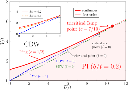
Figure 1: (Color online) iDMRG ground-state phase diagram of the 1D EHM with bond dimerization (2). The red solid line gives the PI-CDW phase boundaries for $\delta/t=0.2$. The quantum phase transition is continuous (first order) below (above) the tricritical Ising point $[U_{\rm t},V_{\rm t}]$ marked by the asterisk. For comparison results for the BOW-CDW (blue dashed line), SDW-BOW (green dotted line), and SDW-CDW (green dashed-dotted line) transitions of the pure EHM ($\delta=0$) were included. Ejima and Nishimoto (2007) (Inset) PI-CDW transition for $\delta/t=0.1$ and $0.2$ in the weak-coupling regime. As expected, decreasing $\delta/t$, the transition lines come closer to BOW-CDW transition line of the pure EHM.

According to weak-coupling renormalization-group results, Tsuchiizu and Furusaki (2004) a bond alternation $\delta$ changes the universality class of the BOW-CDW transition in the EHM from Gaussian- to Ising-type. The Ising criticality has been confirmed by DMRG computations. Benthien et al. (2006)

Figure 1 presents the complete ground-state phase diagram of the EHM with bond dimerization, as obtained by the iDMRG technique. The phase boundaries for the pure EHM are also included (blue and green lines). The dimerized PI phase replaces entirely the SDW and BOW states of the EHM. The PI state has the lowest energy also in the weak-coupling regime, and even at $U/t=0$. This finding confirms previous weak-coupling renormalization group results. Tsuchiizu and Furusaki (2004) In the intermediate-to-strong coupling regime, the PI-CDW transition line converges to those of the BOW/SDW-CDW transition for the pure EHM. The transition is continuous up to the tricritical Ising point $[U_{\rm t},V_{\rm t}](\delta)$, which converges naturally to the tricritical point of the EHM when $\delta\to 0$. Above $[U_{\rm t},V_{\rm t}]$, the PI-CDW transition becomes first order. At very large $U/t$, the phase boundaries of the PI/SDW-CDW transitions are almost indistinguishable.

We now characterize the different ground states of the model (2) in some more detail. Since the dimerized PI state can be considered as an SPT state, the entanglement spectrum plays an important role in our analysis. The so-called entanglement spectrum $\epsilon_{\alpha}$ can be extracted from the singular value decomposition. Lange et al. (2015) Dividing our system into two subblocks, $\cal{H}=\cal{H}_{\textrm{L}}\otimes\cal{H}_{\textrm{R}}$, and considering the reduced density matrix $\rho_{\textrm{L}}=\mathrm{Tr}_{\textrm{R}}[\rho]$, the entanglement spectra are given by the singular values $\lambda_{\alpha}$ of $\rho_{\textrm{L}}$ as $\epsilon_{\alpha}=-2\ln\lambda_{\alpha}$. Moreover, the correlation length $\xi_{\chi}$ can be determined from the second largest eigenvalue of the transfer matrix for some bond dimension $\chi$ used in the iDMRG simulation. McCulloch ; Schollwöck (2011) While the physical correlation length diverges at the critical point, $\xi_{\chi}$ stays finite, as a consequence of working with a finite bond dimension $\chi$. Because of $\xi_{\chi}$’s rapid increase with $\chi$ near the critical point, $\xi_{\chi}$ can be used nevertheless to determine the phase transition. We performed iDMRG simulations with $\chi$ up to 400, so that the effective correlation length at criticality is less or at most equal 300.

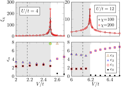
Figure 2: (Color online) Correlation length $\xi_{\chi}$ (top) and entanglement spectrum $\epsilon_{\alpha}$ (bottom) as a function of $V/t$ for $U/t=4$ (left) and $U/t=12$ (right), where $\delta/t=0.2$. Data are obtained by iDMRG. Dashed lines give the BOW-CDW (SDW-CDW) transition for $U/t=4$ ($U/t=12$) in the EHM. Ejima and Nishimoto (2007)

Figure 2 gives $\xi_{\chi}$ and $\epsilon_{\alpha}$ as functions of $V/t$ for fixed $\delta/t=0.2$, at two characteristic $U/t$ values. In the weak-to-intermediate coupling regime, $U/t=4$, we find a distinct peak in the correlation length at $V_{\rm c}/t\simeq 2.504$, which increases rapidly as $\chi$ grows from 100 to 200, indicating the divergence of the correlation length $\xi_{\chi}\to\infty$ as $\chi\to\infty$, i.e., a quantum phase transition (of Ising type, as will be shown in Sec. III.3). In contrast, at strong coupling $U/t=12$, the peak height stays almost constant at $V_{\rm c}/t\simeq 6.194$ when $\chi$ is enhanced. Decreasing the magnitude of $\delta/t$, the transition points will approach those of the pure EHM, e.g., for $\delta/t=0.1$ and $U/t=4$ we find $V_{\rm c}/t\simeq 2.372$, with a simultaneous reduction of the $\xi_{\chi}$’s peak heights. Most notably, the entanglement spectra of the dimerized SPT phase exhibits a distinguishing double degeneracy in the lowest entanglement level; Pollmann et al. (2010) for $V>V_{\rm c}$, in the CDW phase, this level is nondegenerate.

III.2 Excitation gaps

Figure 3: (Color online) Charge ($\Delta_{\rm c}$), spin ($\Delta_{\rm s}$) and neutral ($\Delta_{\rm n}$) gaps in dependence on $V/t$ for (a) $U/t=4$ and (b) $U/t=12$. Again, $\delta/t=0.2$. The dimerized PI (CDW) phase is marked in gray (white). Note the jump of the spin gap, $\delta_{\rm s}\equiv\Delta_{\rm s}(V_{\rm c}^{+})-\Delta_{\rm s}(V_{\rm c}^{-})$, at $V_{\rm c}/t$.

Let us now analyze the behavior of the various excitation gaps. Following previous treatment of the SPT phase, Ejima and Fehske (2015); Lange et al. (2015) we define the spin-, two-particle charge-, and neutral gaps as

$$\Delta_{\rm s} = E_{0}(N,1)-E_{0}(N,0)\,,$$ (4)

$$\Delta_{\rm c} = \frac{1}{2}\{E_{0}(N+2,0)+E_{0}(N-2,0)-2E_{0}(N,0)\}\,,$$

and

$$\Delta_{\rm n}=E_{1}(N,0)-E_{0}(N,0)\,,$$ (6)

respectively. Here, $E_{0}(N_{\rm e},S_{\rm tot}^{z})$ denotes the ground-state energy of the finite system with $L$ sites, given the number of electrons $N_{\rm e}$ and the $z$-component of total spin $S_{\rm tot}^{z}$. $E_{1}(N_{\rm e},S_{\rm tot}^{z})$ is the corresponding energy of the first excited state.

In the pure EHM ($\delta=0$), at small–to–intermediate $U/t$ and $V/t$, both $\Delta_{\rm c}$ and $\Delta_{\rm n}$ vanish at the BOW-CDW transition, whereas $\Delta_{\rm s}$ stays finite. Turning on the dimerization $\delta$, also the charge gap becomes finite, while the neutral gap still closes linearly, reflecting the fact that the transition point belongs to the Ising universality class, see Fig. 3(a) for $U/t=4$, where $V_{\rm c}/t\simeq 2.503$.

By contrast, in the strong-coupling regime, the neutral gap stays finite passing the transition point, see Fig. 3(b) for $U/t=12$. Most strikingly, the spin gap exhibits a jump at the transition point ($V_{\rm c}/t\simeq 6.192$), which indicates a first-order transition.

III.3 Entanglement entropy

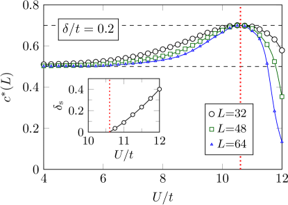
Figure 4: (Color online) Central charge $c^{\ast}(L)$ along the PI-CDW transition line for $\delta/t=0.2$. DMRG data (obtained with PBC) indicate the Ising universality class ($c=1/2$) for $U<U_{\rm t}$ and, most notably, a tricritical Ising point with $c=7/10$ at $U_{\rm t}$ (red dotted line). (Inset) Jump-value of the spin gap for $U\gtrsim U_{\rm t}$. The infinite MPS data point to a first order transition.

We finally determine the universality class of the PI-CDW quantum phase transition. When the system becomes critical, the central charge $c$ can easily be deduced from the entanglement entropy. Ejima et al. (2014); Ejima and Fehske (2015) CFT tells us that the von Neumann entropy for a system with PBC isCalabrese and Cardy (2004)

$$S_{L}(\ell)=\frac{c}{3}\ln\left[\frac{L}{\pi}\sin\left(\frac{\pi\ell}{L}\right)\right]+s_{1}\;,$$ (7)

where $s_{1}$ is a non-universal constant. In the face of the doubled unit cell of the SPT phase the related formula for the central charge should be modified as Nishimoto (2011)

$$c^{\ast}(L)\equiv\frac{3[S_{L}(L/2-2)-S_{L}(L/2)]}{\ln\{\cos[\pi/(L/2)]\}}\;.$$ (8)

Figure 4 displays $c^{\ast}(L)$ along the PI-CDW transition line, varying $U$ and $V$ simultaneously at fixed dimerization strength $\delta/t=0.2$. With increasing $U$, we find clear evidence for a crossover from $c^{\ast}(L)\simeq 1/2$ to $c^{\ast}(L)\simeq 7/10$, which signals Ising tricriticality.

Alternatively, the tricritical Ising point can be estimated from the magnitude of the jump of the spin gap, $\delta_{\rm s}$, see inset of Fig. 3 for $U/t=12$. $\delta_{\rm s}$ should be finite for $U>U_{\rm t}$, and is expected to vanish at the tricritical Ising point, where $U=U_{\rm t}$. This is confirmed by the inset of Fig. 4. Obviously, $\delta_{\rm s}$ closes at $U_{\rm t}/t\simeq 10.6$, in accord with the critical value estimated from the numerically obtained central charge $c^{\ast}(L)$ in the main panel.

IV Field theory analysis

The weak-coupling regime $U$, $V\ll t$ of the model (2) can be analyzed by field theory methods.Tsuchiizu and Furusaki (2004); Benthien et al. (2006) A standard bosonization analysis Gogolin et al. (1999); Essler et al. (2005) leads to the following form of the low-energy Hamiltonian:

$${\cal H} = \sum_{\alpha=\textrm{c},\textrm{s}}\frac{v_{\alpha}}{16\pi}\left[(\partial_{x}\Phi_{\alpha})^{2}+(\partial_{x}\Theta_{\alpha})^{2}\right]+{\cal H}_{\textrm{int}}\,,$$

$${\cal H}_{\textrm{int}} = -\lambda_{\textrm{c}}\cos(\beta_{\textrm{c}}\Phi_{\textrm{c}})$$ (9)

$$+\lambda_{\textrm{s}}\left[\cos\left(\Phi_{\textrm{s}}\right)+\frac{a_{0}^{2}}{16}\left[(\partial_{x}\Theta_{\textrm{s}})^{2}-(\partial_{x}\Phi_{\textrm{s}})^{2}\right]\right]$$

$$+\lambda_{\delta}\cos\left(\frac{\Phi_{\textrm{s}}}{2}\right)\cos\left(\frac{\beta_{\textrm{c}}}{2}\Phi_{\textrm{c}}\right)$$

$$+\lambda_{\delta}^{\prime}\cos\left(\frac{\Phi_{\textrm{s}}}{2}\right)\cos\left(\frac{3\beta_{\textrm{c}}}{2}\Phi_{\textrm{c}}\right)+\dots\,.$$

Here, $a_{0}$ is the lattice spacing, $\Phi_{\rm s,c}$ are canonical Bose fields associated with the collective spin and charge degrees of freedom, and $\Theta_{\rm s,c}$ the associated dual fields fulfilling

$$[\Phi_{\alpha}(x),\Theta_{\alpha^{\prime}}(x^{\prime})]=4\pi i\delta_{\alpha,\alpha^{\prime}}\textrm{sgn}(x-x^{\prime}).$$ (10)

The parameters $\beta_{\rm c}$, $\lambda_{\rm c,s}$, $\lambda_{\delta}$, $\lambda^{\prime}_{\delta}$, $v_{\rm c,s}$ can be determined at weak coupling $U,V,\delta\ll t$. Compared to Ref. [Benthien et al., 2006] we have retained one higher harmonic in the interaction potential between spin and charge degrees of freedom. The reason for this will become clear later on.

IV.1 Quantum critical line

It was shown in Refs. [Tsuchiizu and Furusaki, 2004] and [Benthien et al., 2006] that for appropriate choices of the parameters $U$, $V$, and $\delta$ the spin sector is gapped, while the charge sector undergoes a quantum phase transition. In the vicinity of this critical line we have

$$\cos\left(\frac{\Phi_{\textrm{s}}}{2}\right)\neq 0\,.$$ (11)

Integrating out the massive spin degrees of freedom then leads to an effective low-energy description of the charge sector by a triple sine-Gordon model

$${\cal H}_{\textrm{c}}^{\textrm{eff}} = \frac{v}{16\pi}\left[(\partial_{x}\Phi_{\textrm{c}})^{2}+(\partial_{x}\Theta_{\textrm{c}})^{2}\right]+g_{\delta}\cos\left(\frac{\beta_{\textrm{c}}}{2}\Phi_{\textrm{c}}\right)$$ (12)

$$+g_{\textrm{c}}\cos\left(\beta_{\textrm{c}}\Phi_{\textrm{c}}\right)+g_{\delta}^{\prime}\cos\left(\frac{3\beta_{\textrm{c}}}{2}\Phi_{\textrm{c}}\right)+\dots\,.$$

If we neglect the last term, we arrive at the two-frequency sine-Gordon model discussed in Ref. [Benthien et al., 2006]. It exhibits a quantum phase transition in the Ising universality class. Delfino and Mussardo (1998) In the classical limit $\beta_{\textrm{c}}\to 0$, this corresponds to values of $g_{\textrm{c}}$ and $g_{\delta}$ such that the quadratic terms in the expansion of the cosines precisely cancel. The reason for retaining the last term in (12) is now clear: by fine-tuning the parameters $g_{\rm c}$, $g_{\delta}$, $g^{\prime}_{\delta}$ in the classical limit, we can set the coefficient of the quartic term in the expansion of the interaction potential to zero as well, which corresponds to a phase transition in the tricritical Ising universality class. This scenario is known to persist in the full quantum theory. Tóth (2004)

It is important to note that while the field theories (9) and (12) are initially derived in the limit $U,V,\delta\ll t$, they have a wider regime of applicability, provided that their parameters are adjusted appropriately. In the following we will assume that the description (12) applies along the line of quantum phase transitions even at large values of $U/t$ and $V/t$. This will allow us to make predictions for the large distance behavior of various correlation functions, which then can be tested by numerical computations for the lattice model.

IV.2 Density correlations

In the field theory limit, the bosonized form of the electron density is

$$n_{j}\to\rho_{0}(x)+(-1)^{j}\rho_{\pi}(x)\ ,\quad x=ja_{0}\,,$$ (13)

where

$$\rho_{0}(x) = {\rm const}-\frac{\beta_{\rm c}}{2\pi}\partial_{x}\Phi_{\textrm{c}}+\hat{A}_{0}\partial_{x}\Phi_{\rm c}\cos\big{(}\frac{\Phi_{\rm s}}{2}\big{)}+\dots\,,$$

$$\rho_{\pi}(x) = \hat{A}_{\pi}\sin\left(\frac{\beta_{\textrm{c}}}{2}\Phi_{\textrm{c}}\right)\cos\left(\frac{\Phi_{\textrm{s}}}{2}\right)+\dots\,.$$ (14)

Here we have absorbed Klein factors into the non-universal amplitudes $\hat{A}_{0,\pi}$. Importantly, at half-filling the smooth component $\rho_{0}(x)$ does not contain a $4k_{\rm F}$ umklapp contribution.Controzzi and Essler (2002) As this is quite important, it is worthwhile to review the derivation of this fact. We note that the Hamiltonian (2) is invariant under the particle-hole transformation

$$\hat{C}\hat{c}_{j,\sigma}\hat{C}^{\dagger}=(-1)^{j}\hat{c}_{j,-\sigma}.$$ (15)

The electron density operator is odd under (15)

$$\hat{C}(\hat{n}_{j}-1)\hat{C}^{\dagger}=1-\hat{n}_{j}\,.$$ (16)

In the field theory Eq. (15) is implemented as follows

$$\hat{C}\varphi_{\textrm{c}}\hat{C}^{\dagger} = -\varphi_{\textrm{c}}\,,\ \ \ \hat{C}\bar{\varphi}_{\textrm{c}}\hat{C}^{\dagger}=-\bar{\varphi}_{\textrm{c}}\,,$$

$$\hat{C}\varphi_{\textrm{s}}\hat{C}^{\dagger} = \varphi_{\textrm{s}}\,,\ \ \ \hat{C}\bar{\varphi}_{\textrm{s}}\hat{C}^{\dagger}=\bar{\varphi}_{\textrm{s}}\,,$$

$$\hat{C}\eta_{\sigma}\hat{C}^{\dagger} = \eta_{-\sigma}\,,\ \ \ \hat{C}\bar{\eta}_{\sigma}\hat{C}^{\dagger}=\bar{\eta}_{-\sigma}\,.$$ (17)

Here $\eta_{\uparrow}$, $\eta_{\downarrow}$, $\bar{\eta}_{\downarrow}$, and $\bar{\eta}_{\uparrow}$ are Klein factors, cf. Ref. [Essler et al., 2015]. At general band filling, the $4k_{\textrm{F}}$-term in the charge density takes the form

$$\rho_{4k_{\textrm{F}}}(x)=A_{4k_{\textrm{F}}}\eta_{\uparrow}{\bar{\eta}}_{\uparrow}\eta_{\downarrow}{\bar{\eta}}_{\downarrow}\cos(\beta_{\textrm{c}}\Phi_{\textrm{c}}-4k_{\textrm{F}}x)+\dots\,.$$ (18)

Eq. (17) implies that at half-filling ($4k_{\textrm{F}}x=0\mod 2\pi$) we have

$$C\rho_{4k_{\textrm{F}}}(x)C^{\dagger}=\rho_{4k_{\textrm{F}}}(x)\,,$$ (19)

which can be reconciled with Eq. (16) only by taking $A_{4k_{\textrm{F}}}=0$.

In the vicinity of the quantum critical line, we can again integrate out the gapped spin degrees of freedom and arrive at

$$\rho_{0}(x) = {\rm const}+B_{0}\partial_{x}\Phi_{\textrm{c}}+\dots\ ,$$

$$\rho_{\pi}(x) = B_{\pi}\sin\left(\frac{\beta_{\textrm{c}}}{2}\Phi_{\textrm{c}}\right)+\dots\,.$$ (20)

Finally, we need to relate our charge boson to the primary fields in the tricritical Ising model. This can be done by referring to the Landau-Ginzburg description of the transition, see, e.g., Ref. [Lässig et al., 1991]. Expanding our low-energy effective theory (12) for $\beta_{\rm c}\ll 1$, we obtain the Landau-Ginzburg model

$${\cal L}\sim\frac{v}{16\pi}\Phi_{\rm c}\left(\partial_{x}^{2}-\frac{\partial_{t}^{2}}{v^{2}}\right)\Phi_{\rm c}-\lambda_{2}\Phi_{\rm c}^{2}-\lambda_{4}\Phi_{\rm c}^{4}-\lambda_{6}\Phi_{\rm c}^{6}+\dots.$$ (21)

In this limit, we can then use Ref. [Lässig et al., 1991] to relate local operators in our theory to primary fields in the TIM. In particular, one has

$$\Phi_{\rm c}(x) \leftrightarrow \sigma(x)\ ,$$

$$:\Phi^{2}_{\rm c}(x): \leftrightarrow \epsilon(x)\ ,$$

$$:\Phi^{3}_{\rm c}(x): \leftrightarrow \sigma^{\prime}(x)\ ,$$

$$:\Phi^{4}_{\rm c}(x): \leftrightarrow \epsilon^{\prime}(x)\,,$$ (22)

where $\sigma$, $\epsilon$, $\sigma^{\prime}$, and $\epsilon^{\prime}$ are respectively the magnetization field, energy density, sub-magnetization, and vacancy density in the TIM. Proceeding in the same way for the components of the charge density (20) then suggests the following identifications:

$$\rho_{\pi}(x) \sim A\sigma(x)+\dots\,,$$

$$\rho_{0}(x) \sim {\rm const}+Ba_{0}\partial_{x}\sigma(x)+\dots\,.$$ (23)

Using the known results for correlation functions in the TIM, we then arrive at the following prediction for the density-density correlator at the Ising tricritical point:

$$\langle(\hat{n}_{j+\ell}-1)(\hat{n}_{j}-1)\rangle\sim(-1)^{\ell}\frac{A^{2}}{\ell^{3/20}}+\dots\,,\ \ell\gg 1.$$ (24)

We may isolate the subleading behavior by considering smooth and staggered combinations of the density on the lattice:

$$\hat{n}_{j}^{\rm st} = (-1)^{j}(\hat{n}_{j}-\hat{n}_{j+1})\sim 2A\sigma(x)+\dots\,,$$

$$\hat{n}_{j}^{\rm sm} = \frac{\hat{n}_{j}+\hat{n}_{j+1}}{2}-1\sim(B-(-1)^{j}A)a_{0}\partial_{x}\sigma+\dots\,.$$

The TIM predictions for two point functions of these operators are

$$\langle\hat{n}_{j+\ell}^{\rm st}\hat{n}_{j}^{\rm st}\rangle \sim 4A^{2}\ell^{-3/20}+\dots\,,$$ (26)

$$\langle\hat{n}_{j+\ell}^{\rm sm}\hat{n}_{j}^{\rm sm}\rangle \sim C_{j,\ell}\ell^{-43/20}+\ldots\ ,$$

$$C_{j,\ell} = -\frac{69}{400}\begin{cases}B^{2}-A^{2}/4&\ell\text{ odd}\\ [B-(-1)^{j}A/2]^{2}&\ell\text{ even.}\end{cases}$$ (27)

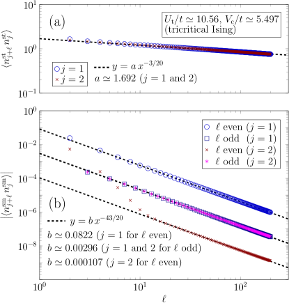
Figure 5: (Color online) Density-density correlation functions at the tricritical Ising point for $\delta/t=0.2$. Data obtained by iDMRG with $\chi=1600$. The correlation functions (symbols) show a power-law decay, in accordance with the field theory predictions, Eqs. (26) and (27).

The predictions (26) and (27) can now be compared with iDMRG simulations of the 1D lattice model (2). Figure 5 shows the iDMRG results for two point functions of the (a) staggered and (b) smooth combinations of the particle density at the TIM critical point of the lattice model. The results for $\langle\hat{n}_{j+\ell}^{\rm st}\hat{n}_{j}^{\rm st}\rangle$ are seen to be in excellent agreement with the leading $\ell^{-3/20}$ dependence at long distances predicted by Eq. (26) for both $j=1$ and $j=2$. To test the second prediction in Eq. (27), we consider separately the cases of even and odd $\ell$ for $j=1$ and $j=2$, and plot the absolute value of $\langle\hat{n}_{\ell+1}^{\rm sm}\hat{n}_{1}^{\rm sm}\rangle$ in Fig. 5(b). Again the numerical data are seen to be in excellent agreement with the predicted $\ell^{-43/20}$ dependence at large separations. The prefactors for the power laws extracted from our iDMRG data are in very good agreement with the prediction of Eq. (27) as well.

IV.3 BOW correlations

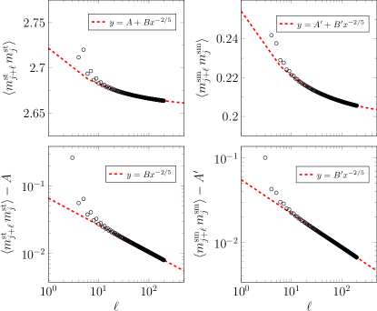
Figure 6: (Color online) BOW correlation functions at the tricritical Ising point for $\delta/t=0.2$ computed by iDMRG with $\chi=1600$. (Top) The asymptotic values for the two-point functions of staggered and smooth combinations of the BOW density are estimated by fitting to Eqs. (33) and (34). (Bottom) log-log plots of the same correlation functions with the asymptotic values subtracted show power-law decay compatible with Ising tricriticality.

The BOW order parameter is given by $\hat{m}_{\rm BOW}=(1/L)\sum_{j}\hat{m}_{j}$ with

$$\hat{m}_{j}=(-1)^{j}\sum_{\sigma}\left[\hat{c}_{j\sigma}^{\dagger}\hat{c}_{j+1\sigma}^{\phantom{\dagger}}+{\rm h.c.}\right]\,.$$ (28)

The BOW order parameter is always non-zero in the vicinity of the transition

$$\langle\hat{m}_{\rm BOW}\rangle\neq 0.$$ (29)

The bosonized expression for $\hat{m}_{\rm BOW}$ is

$$\hat{m}_{j} \sim (-1)^{j}{\rm const}+\hat{C}_{\pi}\cos\left(\frac{\beta_{\textrm{c}}}{2}\Phi_{\textrm{c}}\right)\cos\left(\frac{\Phi_{\textrm{s}}}{2}\right)$$ (30)

$$+(-1)^{j}\hat{C}_{0}\cos\big{(}\beta_{\rm c}\Phi_{\rm c}\big{)}+\dots.$$

We now proceed in the same way as for the charge density. We integrate out the gapped spin degrees of freedom, then expand for small $\beta_{\rm c}$, and finally use the Landau-Ginzburg description to identify which operators in the TIM dominate the long distance behavior of the BOW correlations. The main difference compared to the charge density is that the BOW order parameter is even under charge conjugation, and concomitantly we find

$$\hat{m}_{j} \sim \langle\hat{m}_{\rm BOW}\rangle+D_{0}\epsilon(x)$$ (31)

$$+(-1)^{j}\left[D_{1}+D_{2}\epsilon(x)\right]+\ldots\ .$$

We again form smooth and staggered combinations,

$$\hat{m}_{j}^{\rm st} = (-1)^{j}(\hat{m}_{j}-\hat{m}_{j+1})\sim 2\left[D_{1}+D_{2}\epsilon(x)\right]+\dots\,,$$

$$\hat{m}_{j}^{\rm sm} = \frac{\hat{m}_{j}+\hat{m}_{j+1}}{2}\sim\langle\hat{m}_{\rm BOW}\rangle+D_{0}\epsilon(x)+\dots\,.$$ (32)

The TIM predictions for BOW correlations are then

$$\langle\hat{m}_{j+\ell}^{\rm st}\hat{m}_{j}^{\rm st}\rangle \sim 4\left[D_{1}^{2}+D_{2}^{2}\ell^{-2/5}\right]+\dots\,,$$ (33)

$$\langle\hat{m}_{j+\ell}^{\rm sm}\hat{m}_{j}^{\rm sm}\rangle \sim \langle\hat{m}_{\rm BOW}\rangle^{2}+D_{0}^{2}\ell^{-2/5}+\dots\,.$$ (34)

These predictions can be compared to iDMRG computations in Fig. 6. In order to remove the constant terms in Eqs. (33) and (34), we first fit the numerical results to the functional form $y=A+Bx^{-2/5}$. This allows us to extract the constants as shown in the upper panels in Fig. 6. Subtracting the estimated constants from original data, both staggered and smooth correlation functions are seen to decay in a power-law fashion compatible with the TIM prediction.

IV.4 Spin correlations

As the spin sector is gapped, we expect an exponential decay for the spin two-point function

$$\langle\hat{S}^{z}_{j+\ell}\hat{S}^{z}_{j}\rangle\sim E_{0}e^{-\ell/\xi_{1}}+E_{1}(-1)^{\ell}e^{-\ell/\xi_{2}}\,.$$ (35)

Here we have used that the low energy degrees of freedom in the spin sector occur at wave numbers zero and $\pi$. This behavior is again in good agreement with iDMRG computations as shown in Fig. 7. The correlation lengths extracted by fitting the iDMRG results to Eq. (35) are found to be in reasonable agreement with the corresponding eigenvalue of the transfer matrix $\xi_{1}\simeq 1.225$.

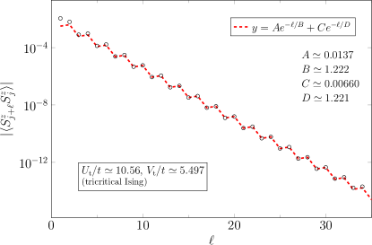
Figure 7: (Color online) Spin correlation function (symbols) at the tricritical Ising point for $\delta/t=0.2$ using the iDMRG with $\chi=1600$, showing exponential decay. The line is a fit to Eq. (35).

To summarize this section, we have seen that field theory predictions obtained by means of a triple sine-Gordon model description of the tricritical Ising transition are in excellent agreement with iDMRG computations for the lattice model. This firmly establishes that the critical endpoint is in the universality class of the TIM. We note that an analogous field theory description applies along the entire Ising critical line. Here, field theory predictions are again in excellent agreement with iDMRG computations as shown in Appendix.

V Conclusions

We have revisited ground-state properties of the one-dimensional half-filled extended Hubbard model with staggered bond dimerization. We have employed a combination of numerical and analytical techniques to map out the ground-state phase diagram in detail, and identify all quantum critical regions. At fixed dimerization $\delta$, there are two distinct phases. A CDW phase at large $V\gtrsim U$ is separated from a PI phase at $U\gtrsim V$ by an Ising critical line, that terminates in a critical point which we have shown to be in the universality class of the tricritical Ising model. Our identification was based on a detailed analysis of both entanglement entropy scaling and critical exponents describing the power-law decay of several two-point correlation functions.

Correlation functions of local operators in the EHM with bond dimerization access only the bosonic sector of the TIM CFT. This precludes us from directly investigating the emergence of supersymmetry at low energies/long distances. To “see” the fermionic sector one presumably would have to consider correlation functions of suitably constructed non-local operators. It would be interesting to investigate this possibility further. Another issue worth pursuing is to investigate the scaling regime around the TIM critical point in the framework of the EHM with bond dimerization. It would be interesting to investigate whether it is possible to make contact with the field theory predictions of Ref. [Lepori et al., ].

Appendix A Correlation functions on the Ising critical line

The tricritical Ising model describes the end point of a critical line of Ising transitions, cf. Fig. 1. The Ising critical line was previously investigated by DMRG methods in Ref. [Benthien et al., 2006] and the critical exponents were extracted by considering the scaling of the order parameter and spectral gap in the vicinity of the transition. In this appendix we complement these results by examining the power law behavior of correlations functions at the transition, i.e. the same diagnostics we used in the main text to identify the TIM critical point.

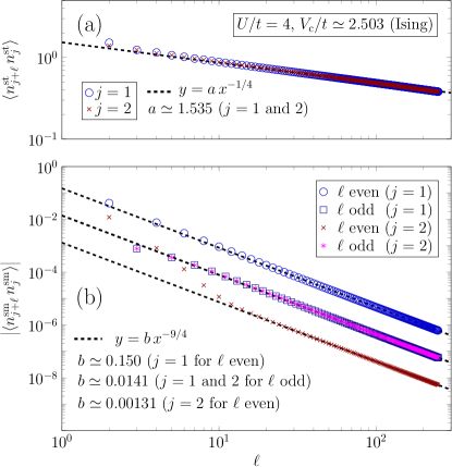
Figure 8: (Color online) Density-density correlation functions at the Ising transition point ($V_{\rm c}\simeq 2.503$) for $U/t=4$ and $\delta/t=0.2$, using the iDMRG with $\chi=1600$. (a) The correlator of the staggered combination is in excellent agreement with Eq. (37) with $4\tilde{A}^{2}\approx 1.535$. (b) Correlations of the smooth combination $n^{\rm sm}_{j}$ are plotted separately for odd and even $\ell$ with $j=1$ and 2. The data are in excellent agreement with the prediction Eq. (38).

The identification of operators is analogous to the TIM case. The projections of the particle density and BOW order parameter onto local fields in the Ising CFT are again of the form (23) and (32), but $\sigma(x)$ and $\epsilon(x)$ are now the spin field and energy density of the Ising CFT. This leads to the following prediction for the large distance asymptotics of the density-density correlator

$$\langle(\hat{n}_{j+\ell}-1)(\hat{n}_{j}-1)\rangle \sim (-1)^{\ell}\tilde{A}\ell^{-1/4}+\dots\,.$$ (36)

Considering smooth and staggered combinations defined in (LABEL:local-n-stsm) separately, we obtain

$$\langle\hat{n}_{j+\ell}^{\rm st}\hat{n}_{j}^{\rm st}\rangle \sim 4\tilde{A}^{2}\ell^{-1/4}+\dots\,,$$ (37)

$$\langle\hat{n}_{j+\ell}^{\rm sm}\hat{n}_{j}^{\rm sm}\rangle \sim \tilde{C}_{j,\ell}\ell^{-9/4}+\ldots\ ,$$

$$\tilde{C}_{j,\ell} = -\frac{5}{16}\begin{cases}\tilde{B}^{2}-\tilde{A}^{2}/4&\ell\text{ odd}\\ [\tilde{B}-(-1)^{j}\tilde{A}/2]^{2}&\ell\text{ even.}\end{cases}$$ (38)

These predictions are in excellent agreement with iDMRG computations for the lattice model on the Ising critical line as is shown in Fig. 8.

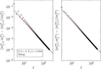
Figure 9: (Color online) BOW correlations at the Ising transition point for $U/t=4$ and $\delta/t=0.2$. The correlators exhibit a power-law decay consistent with the field theory predictions, Eqs. (39).

The field theory predictions for staggered and smooth combinations of the BOW order parameter on the Ising transition line are

$$\langle\hat{m}_{j+\ell}^{\rm st}\hat{m}_{j}^{\rm st}\rangle \sim (-1)^{\ell}\left[\tilde{C}_{4}^{2}+\tilde{C}_{5}\ell^{-2}\right]+\dots\,,$$

$$\langle\hat{m}_{j+\ell}^{\rm sm}\hat{m}_{j}^{\rm sm}\rangle \sim \langle\hat{m}_{\rm BOW}\rangle^{2}+\tilde{C}_{6}\ell^{-2}+\dots\,.$$ (39)

We can remove the constant contributions by considering connected correlators, which in turn exhibit power-law decay to zero at large distances. The iDMRG results shown in Fig. 9 agree perfectly with the predicted $\ell^{-2}$ power-law decay. As a consistency check we have extracted the value of $\langle\hat{m}_{\rm BOW}\rangle$ by fitting the long-distance behavior of two-point function of $\hat{m}_{j}^{\rm sm}$ to the form (39). We find it to be in excellent agreement with the value obtained by computing the one-point function.

We note that the agreement between our numerical data and field theory predictions is much better along the Ising transition line that at the TIM critical point. There are two reasons for this. First, at fixed $U/t$, the Ising transition point ($V_{\rm c}/t$) can be determined more accurately than the location of the TIM transition, where two parameters ($U$ and $V$) have to be fine-tuned simultaneously. Second, the corrections to scaling are different in both cases.

References

- Friedan et al. (1984) D. Friedan, Z. Qiu, and S. Shenker, Phys. Rev. Lett. 52, 1575 (1984).
- Friedan et al. (1985) D. Friedan, Z. Qiu, and S. Shenker, Physics Letters B 151, 37 (1985).
- Blume (1966) M. Blume, Phys. Rev. 141, 517 (1966).
- Capel (1966) H. Capel, Physica (Amsterdam) 32, 966 (1966).
- Alcaraz et al. (1985) F. C. Alcaraz, J. R. Drugowich de Felício, R. Köberle, and J. F. Stilck, Phys. Rev. B 32, 7469 (1985).
- Feiguin et al. (2007) A. Feiguin, S. Trebst, A. W. W. Ludwig, M. Troyer, A. Kitaev, Z. Wang, and M. H. Freedman, Phys. Rev. Lett. 98, 160409 (2007).
- Rahmani et al. (2015) A. Rahmani, X. Zhu, M. Franz, and I. Affleck, Phys. Rev. Lett. 115, 166401 (2015).
- Zhu and Franz (2016) X. Zhu and M. Franz, Phys. Rev. B 93, 195118 (2016).
- Lange et al. (2015) F. Lange, S. Ejima, and H. Fehske, Phys. Rev. B 92, 041120 (2015).
- Pollmann et al. (2010) F. Pollmann, A. M. Turner, E. Berg, and M. Oshikawa, Phys. Rev. B 81, 064439 (2010).
- Tsuchiizu and Furusaki (2004) M. Tsuchiizu and A. Furusaki, Phys. Rev. B 69, 035103 (2004).
- Benthien et al. (2006) H. Benthien, F. H. L. Essler, and A. Grage, Phys. Rev. B 73, 085105 (2006).
- Nakamura (1999) M. Nakamura, J. Phys. Soc. Jpn. 68, 3123 (1999).
- Nakamura (2000) M. Nakamura, Phys. Rev. B 61, 16377 (2000).
- White (1992) S. R. White, Phys. Rev. Lett. 69, 2863 (1992).
- Gogolin et al. (1999) A. O. Gogolin, A. A. Nersesyan, and A. M. Tsvelik, Bosonization and Strongly Correlated Systems (Cambridge University Press, Cambridge, 1999).
- Essler et al. (2005) F. H. L. Essler, H. Frahm, F. Göhmann, A. Klümper, and V. E. Korepin, The One-Dimensional Hubbard Model (Cambridge University Press, Cambridge, 2005).
- Sengupta et al. (2002) P. Sengupta, A. W. Sandvik, and D. K. Campbell, Phys. Rev. B 65, 155113 (2002).
- Sandvik et al. (2004) A. W. Sandvik, L. Balents, and D. K. Campbell, Phys. Rev. Lett. 92, 236401 (2004).
- Zhang (2004) Y. Z. Zhang, Phys. Rev. Lett. 92, 246404 (2004).
- Tam et al. (2006) K.-M. Tam, S.-W. Tsai, and D. K. Campbell, Phys. Rev. Lett. 96, 036408 (2006).
- Ejima and Nishimoto (2007) S. Ejima and S. Nishimoto, Phys. Rev. Lett. 99, 216403 (2007).
- Giamarchi (2003) T. Giamarchi, Quantum Physics in One Dimension (Oxford University Press, Oxford, 2003).
- Gebhard et al. (1997) F. Gebhard, K. Bott, M. Scheidler, P. Thomas, and S. W. Koch, Phil. Mag. B 75, 1 (1997).
- Nakano and Fukuyama (1981) T. Nakano and H. Fukuyama, J. Phys. Soc. Jpn. 50, 2489 (1981).
- Tsvelik (1992) A. M. Tsvelik, Phys. Rev. B 45, 486 (1992).
- Uhrig and Schulz (1996) G. S. Uhrig and H. J. Schulz, Phys. Rev. B 54, R9624 (1996).
- Essler et al. (1997) F. H. L. Essler, A. M. Tsvelik, and G. Delfino, Phys. Rev. B 56, 11001 (1997).
- Ejima et al. (2006) S. Ejima, F. Gebhard, and S. Nishimoto, Phys. Rev. B 74, 245110 (2006).
- (30) A. Grage, F. Gebhard, and J. Rissler, J. Stat. Mech.: Theory and Exp. (2005), P08009.
- Dzierzawa and Mocanu (2005) M. Dzierzawa and C. Mocanu, J. Phys.: Condens. Matter 17, 2663 (2005).
- Sugiura and Suzumura (2002) M. Sugiura and Y. Suzumura, J. Phys. Soc. Jpn. 71, 697 (2002).
- Tsuchiizu and Orignac (2002) M. Tsuchiizu and E. Orignac, J. Phys. Chem. Solids 63, 1459 (2002).
- (34) I. P. McCulloch, arXiv:0804.2509.
- Schollwöck (2011) U. Schollwöck, Ann. Phys. 326, 96 (2011).
- Ejima and Fehske (2015) S. Ejima and H. Fehske, Phys. Rev. B 91, 045121 (2015).
- Ejima et al. (2014) S. Ejima, F. Lange, and H. Fehske, Phys. Rev. Lett. 113, 020401 (2014).
- Calabrese and Cardy (2004) P. Calabrese and J. Cardy, J. Stat. Mech.: Theory and Exp. (2004), P06002.
- Nishimoto (2011) S. Nishimoto, Phys. Rev. B 84, 195108 (2011).
- Delfino and Mussardo (1998) G. Delfino and G. Mussardo, Nuclear Physics B 516, 675 (1998).
- Tóth (2004) G. Z. Tóth, J. Phys. A: Math. Gen. 37, 9631 (2004).
- Controzzi and Essler (2002) D. Controzzi and F. H. L. Essler, Phys. Rev. B 66, 165112 (2002).
- Essler et al. (2015) F. H. L. Essler, R. G. Pereira, and I. Schneider, Phys. Rev. B 91, 245150 (2015).
- Lässig et al. (1991) M. Lässig, G. Mussardo, and J. L. Cardy, Nucl. Phys. B 348, 591 (1991).
- (45) L. Lepori, G. Mussardo, and G. Z. Tóth, J. Stat. Mech. (2008), P09004.
- (46) http://itensor.org/.