The first spectropolarimetric monitoring of the peculiar O4 Ief supergiant $\zeta$ Puppis

Abstract

The origin of the magnetic field in massive O-type stars is still under debate. To model the physical processes responsible for the generation of O star magnetic fields, it is important to understand whether correlations between the presence of a magnetic field and stellar evolutionary state, rotation velocity, kinematical status, and surface composition can be identified. The O4 Ief supergiant $\zeta$ Pup is a fast rotator and a runaway star, which may be a product of a past binary interaction, possibly having had an encounter with the cluster Trumper 10 some 2 Myr ago. The currently available observational material suggests that certain observed phenomena in this star may be related to the presence of a magnetic field. We acquired spectropolarimetric observations of $\zeta$ Pup with FORS 2 mounted on the 8-m Antu telescope of the VLT to investigate if a magnetic field is indeed present in this star. We show that many spectral lines are highly variable and probably vary with the recently detected period of 1.78 d. No magnetic field is detected in $\zeta$ Pup, as no magnetic field measurement has a significance level higher than 2.4$\sigma$. Still, we studied the probability of a single sinusoidal explaining the variation of the longitudinal magnetic field measurements.

1 Introduction

Magnetic fields in massive stars have fundamental effects on the stellar evolution and rotation, and on the structure, dynamics and heating of their radiatively-driven winds. To identify and to model the physical processes responsible for the generation of their magnetic fields, it is important to establish whether magnetic fields can also be detected in massive stars that are fast rotators and have runaway status. Recent detections of strong magnetic fields in very fast rotating early-B type stars indicate that the spindown timescale via magnetic braking can be much longer than the estimated age of these targets (e.g. Rivinius et al. 2013). Furthermore, current studies of their kinematical status identified a number of magnetic O and Of?p stars as candidate runaway stars (e.g. Hubrig, Kharchenko, & Schöller 2011). Increasing the known number of magnetic objects with extreme rotation, which are probably products of a past binary interaction, is important to understand the magnetic field origin in massive stars.

A few years ago, we presented the first spectropolarimetric observations of $\zeta$ Oph (Hubrig, Oskinova, & Schöller, 2011), obtained with FORS 1 (FOcal Reducer low dispersion Spectrograph; Appenzeller et al. 1998) mounted on the 8-m Kueyen telescope of the Very Large Telescope (VLT). The star $\zeta$ Ophiuchi (=HD 149757) of spectral type O9.5V is a well-known rapidly rotating runaway star, rotating almost at break-up velocity with $v\,\sin\,i=400$ km s^-1 (Kambe, Ando, & Hirata, 1993). Later, additional nine FORS 2 spectropolarimetric observations of $\zeta$ Oph were obtained over four consecutive nights. The analysis of the FORS 2 observations showed the presence of a weak magnetic field with a reversal of polarity (Hubrig et al., 2013) and an amplitude of about 100 G. The resulting periodogram for the magnetic field measurements using all available lines showed a dominating peak corresponding to a period of about 1.3 d, which is roughly double the period of 0.643 d determined by Pollmann (2012), who studied the variation of the equivalent width of the He i 6678 line. David-Uraz et al. (2014) used ESPaDOnS and NARVAL observations of $\zeta$ Oph in 2011/12 with much larger uncertainties – typically around 350 G and between 100 and 800 G – and concluded that the upper limit of the dipole field strength is about 224 G and the maximum possible rotation period 1.1 d. High-resolution spectropolarimetric results are thus in contradiction with the FORS 2 observations.

The O4 Ief supergiant $\zeta$ Pup (=HD 66811) is the brightest O-type star in the sky with a magnitude $V=2.25$. Similar to $\zeta$ Ophiuchi, it rotates rather fast with $v\,\sin\,i=208$ km s^-1 (Conti & Ebbets, 1977), and is a runaway star, which may be a product of a past binary interaction, possibly having had an encounter with the cluster Trumper 10 some 2 Myr ago (Hoogerwerf, de Bruijne, & de Zeeuw, 2001; Schilbach & Röser, 2008). The most recent periodicity analysis was presented by Howarth & Stevens (2014), who determined $P=1.780938\pm 0.000093$ d using optical photometry obtained with the SMEI (Solar Mass Ejection Imager) instrument on the Coriolis satellite between 2003 and 2006. On the other hand, numerous studies in the past that used observations in a different part of the electromagnetic spectrum, reported various periodic or cyclical signals, from a couple of hours to about 5 days. An overview of these studies is presented in the work of Howarth & Stevens (2014). The authors report that no evidence for persistent coherent signals with semi-amplitudes in excess of about 2 mmag on any of the time-scales previously reported in the literature was detected in their data. In particular, there was no evidence for a signature of a rotation period of about 5 d. Noteworthy, the period of 1.78 d was also recently unambiguously identified in observations of the BRITE (BRIght-star Target Explorer) satellites (Ramiaramanantsoa, priv. comm.).

The peculiar behaviour, in particular the appearance of a double-peaked He ii $\lambda$4686 emission line in the spectra of $\zeta$ Pup was already discussed over the last decades (e.g. Conti & Leep 1974). Harries (2000), Harries, Howarth, & Evans (2002), and Vink et al. (2009) reported the presence of complex linear polarization effects across the H$\alpha$ line profiles of $\zeta$ Pup and suggested that they can be attributed to the impact of the rapid rotation of the star on its winds. Moffat & Michaud (1981) detected profile variability with a period of 5.075 d in the depth of the nearly central absorption reversal of the P Cygni type H$\alpha$ profile in spectrophotometric observations of $\zeta$ Pup and proposed that the winds of Oef stars might be shaped by a dipolar stellar magnetic field. Searches for the presence of a magnetic field in $\zeta$ Pup were reported by Chesneau & Moffat (2002) and David-Uraz et al. (2014). Chesneau & Moffat (2002) used CASPEC observations on four consecutive nights, covering time intervals between 30 and 76 min. The measurements were based on four He lines placed well within the CASPEC orders and not sensitive to defects in the normalization procedure. Although a change of field polarity was indicated on every second night, the measurement accuracies were low, between 200 and 360 G. David-Uraz et al. (2014) obtained 30 individual measurements over 1.9 h with ESPaDOnS in a single night. From these observations, the authors estimated an upper limit on the dipolar field strength of 121 G. On the other hand, high-resolution spectropolarimetric observations are not especially appropriate for the detection of weak magnetic fields in broad-lined stars. Some broad spectral lines like the He ii 4686 line or the close-by blend of N iii lines extend over adjacent orders, so that it is necessary to adopt the order shapes to get the best continuum normalization. No continuum normalization is required in FORS 2 spectropolarimetric observations.

Furthermore, it is of importance that Baade (1986) and Reid & Howarth (1996) reported the presence of velocity-resolved structure in the photospheric absorption lines of $\zeta$ Pup, with a possible 8.5-h periodicity. Their observations showed characteristic blue-to-red migration of bumps and dips in the absorption-line profiles, suggesting non-radial pulsation as the underlying physical mechanism. Baade (1986) also mentioned that every 0.178 d a new component develops in the blue wings of the C iv 5801, 5812 lines and it takes twice the amount of time for the feature to traverse the entire profile. Notably, Eversberg et al. (1998) report on the presence of variable substructures on a time scale of 10-20 min, likely representing the stochastic manifestation of turbulent clumps propagating outward with the wind. These studies underline the possible impact of short-time variability on the magnetic field measurements, which can be quite significant in supergiants (see Fig. 5 and e.g. Hubrig, Schöller, & Kholtygin 2014).

Since the information on the presence of a magnetic field in $\zeta$ Pup is rather limited, we decided to carry out spectropolarimetric observations randomly distributed over a few weeks using the VLT instrument FORS 2 in service mode. In this paper, we present the results of our FORS 2 spectropolarimetric monitoring of $\zeta$ Pup and discuss the observed magnetic and spectral variability assuming the oblique rotator interpretation.

2 Magnetic field measurements

Thirteen spectropolarimetric observations of $\zeta$ Pup were carried out from 2013 October 5 to 2013 December 23 in service mode at the European Southern Observatory using FORS 2 (Appenzeller et al., 1998) mounted on the 8-m Antu telescope of the VLT. This multi-mode instrument is equipped with polarisation analysing optics comprising super-achromatic half-wave and quarter-wave phase retarder plates, and a Wollaston prism with a beam divergence of 22$\arcsec$ in standard resolution mode. We used the GRISM 600B and the narrowest available slit width of 0$\farcs$4 to obtain a spectral resolving power of $R\sim 2000$. The observed spectral range from 3250 to 6215 Å includes all Balmer lines, apart from H$\alpha$, down to H14, and numerous helium lines, up to 15. For the observations, we used a non-standard readout mode with low gain (200kHz,1$\times$1,low), which provides a broader dynamic range, hence allowed us to reach a higher signal-to-noise ratio (SNR) in the individual spectra.

A first description of the assessment of the longitudinal magnetic field measurements using FORS 1/2 spectropolarimetric observations was presented in our previous work (e.g. Hubrig et al. 2004a, b, and references therein). To minimize the cross-talk effect, and to cancel errors from different transmission properties of the two polarised beams, a sequence of subexposures at the retarder position angles $-$45^∘$+$45^∘, $+$45^∘$-$45^∘, $-$45^∘$+$45^∘, etc. is usually executed during observations. Moreover, the reversal of the quarter wave plate compensates for fixed errors in the relative wavelength calibrations of the two polarised spectra. According to the FORS User Manual, the $V/I$ spectrum is calculated using:

$$\frac{V}{I}=\frac{1}{2}\left\{\left(\frac{f^{\rm o}-f^{\rm e}}{f^{\rm o}+f^{\rm e}}\right)_{-45^{\circ}}-\left(\frac{f^{\rm o}-f^{\rm e}}{f^{\rm o}+f^{\rm e}}\right)_{+45^{\circ}}\right\}$$ (1)

where $+45^{\circ}$ and $-45^{\circ}$ indicate the position angle of the retarder waveplate and $f^{\rm o}$ and $f^{\rm e}$ are the ordinary and extraordinary beams, respectively. Rectification of the $V/I$ spectra was performed in the way described by Hubrig, Schöller, & Kholtygin (2014). Null profiles, $N$, are calculated as pairwise differences from all available $V$ profiles. From these, 3$\sigma$-outliers are identified and used to clip the $V$ profiles. This removes spurious signals, which mostly come from cosmic rays, and also reduces the noise. A full description of the updated data reduction and analysis will be presented in a separate paper (Schöller et al., in preparation). Due to the brightness of the star, the exposure time for each subexposure accounted for 0.25 s.

The mean longitudinal magnetic field, $\left<B_{\rm z}\right>$, is measured on the rectified and clipped spectra based on the relation

$$\frac{V}{I}=-\frac{g_{\rm eff}\,e\,\lambda^{2}}{4\pi\,m_{\rm e}\,c^{2}}\,\frac{1}{I}\,\frac{{\rm d}I}{{\rm d}\lambda}\left<B_{\rm z}\right>\,,$$ (2)

where $V$ is the Stokes parameter that measures the circular polarization, $I$ is the intensity in the unpolarized spectrum, $g_{\rm eff}$ is the effective Landé factor, $e$ is the electron charge, $\lambda$ is the wavelength, $m_{\rm e}$ is the electron mass, $c$ is the speed of light, ${{\rm d}I/{\rm d}\lambda}$ is the wavelength derivative of Stokes $I$, and $\left<B_{\rm z}\right>$ is the mean longitudinal (line-of-sight) magnetic field (e.g. Angel & Landstreet 1970).

The longitudinal magnetic field was measured in three ways: using the entire spectrum including all available lines, excluding lines in emission, and using exclusively hydrogen lines. The feasibility of longitudinal magnetic field measurements in massive stars using low-resolution spectropolarimetric observations was demonstrated by previous studies of O and B-type stars (e.g., Hubrig et al. 2006, 2008, 2009, 2011, 2013, 2015a). A number of discrepancies in the published measurement accuracies using FORS 1 data were reported by Bagnulo et al. (2012), who used the ESO FORS 1 pipeline to reduce the FORS 1 archive. Some of the reasons for higher error bars in the study of Bagnulo et al. (2012) are discussed by Hubrig et al. (2016). Furthermore, we have carried out Monte Carlo bootstrapping tests. These are most often applied with the purpose of deriving robust estimates of standard errors. The measurement uncertainties obtained before and after Monte Carlo bootstrapping tests were found to be in close agreement, indicating the absence of reduction flaws. Since Baade (1986) and Reid & Howarth (1996) suggested the presence of non-radial pulsations in $\zeta$ Pup, to check the stability of the spectral lines along the full sequence of sub-exposures, we have compared the profiles of several spectral lines recorded in the parallel beam with the retarder waveplate at $+45^{\circ}$. The same was done for spectral lines recorded in the perpendicular beam. The line profiles looked identical within the noise and no instability like that found in the A0 supergiant HD 92207 (Hubrig, Schöller, & Kholtygin, 2014) was found in our FORS 2 observations.

Table 1: Logbook of the FORS 2 polarimetric observations of $\zeta$ Pup, including the modified Julian date of mid-exposure followed by the achieved signal-to-noise ratio in the Stokes $I$ spectrum around 5000 Å, and the measurements of the mean longitudinal magnetic field using the Monte Carlo bootstrapping test, for all lines, excluding the lines in emission, and for the hydrogen lines. In the last columns, we present the results of our measurements using the null spectra and the phases calculated relative to the zero phase corresponding to the negative field extremum at MJD56570.2611. All quoted errors are 1$\sigma$ uncertainties.

MJD	SNR5000	$\left<B_{\rm z}\right>_{\rm all}$		$\left<B_{\rm z}\right>_{\rm no\,emiss}$		$\left<B_{\rm z}\right>_{\rm hydr}$		$\left<B_{\rm z}\right>_{\rm N}$		Phase
		[G]		[G]		[G]		[G]
56570.3265	934	$-$420$\pm$	178	$-$441$\pm$	181	$-$372$\pm$	259	$-$32$\pm$	190	0.037
56622.3478	2396	25$\pm$	61	61$\pm$	65	99$\pm$	139	3$\pm$	71	0.247
56629.2268	2628	4$\pm$	67	$-$12$\pm$	71	$-$24$\pm$	110	$-$2$\pm$	60	0.110
56630.2214	4013	110$\pm$	60	171$\pm$	77	147$\pm$	106	33$\pm$	48	0.668
56631.2471	3428	2$\pm$	44	53$\pm$	46	26$\pm$	91	$-$6$\pm$	55	0.244
56632.1923	2781	$-$12$\pm$	77	$-$44$\pm$	67	$-$77$\pm$	104	$-$27$\pm$	88	0.775
56643.1478	2137	$-$67$\pm$	60	$-$78$\pm$	72	$-$50$\pm$	149	74$\pm$	86	0.926
56644.2183	2337	22$\pm$	91	18$\pm$	101	62$\pm$	136	$-$33$\pm$	93	0.527
56646.0849	2373	132$\pm$	72	148$\pm$	78	122$\pm$	138	$-$59$\pm$	78	0.575
56647.1013	2222	34$\pm$	91	4$\pm$	94	$-$110$\pm$	134	$-$31$\pm$	106	0.146
56647.2830	2365	$-$17$\pm$	47	1$\pm$	57	68$\pm$	146	$-$9$\pm$	60	0.248
56648.2853	2371	34$\pm$	82	47$\pm$	101	51$\pm$	134	$-$17$\pm$	102	0.811
56649.1691	2175	98$\pm$	97	92$\pm$	110	142$\pm$	137	17$\pm$	98	0.307

The results of our magnetic field measurements, those for absorption and emission lines combined, absorption lines alone, and hydrogen lines are presented in Table 1, where we also collect information about the modified Julian date for the middle of the exposure, the achieved peak signal-to-noise ratio in the Stokes $I$ spectrum close to 5000 Å, the measurements obtained using null spectra for the set of all lines, and the rotation phase assuming a rotation period of 1.780938 d. The results using null spectra for the other sets of lines are similar. The first measurement in Table 1 shows the strongest longitudinal magnetic field of about $-400$ G. However, the accuracy is very low due to the low SNR obtained for this observation. In addition, the time interval between this first measurement and the second is the largest, amounting to almost 52 d, while all other measurements were obtained within 27 d.

3 Magnetic and spectral variability

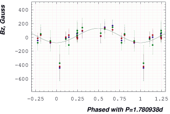
Figure 1: Longitudinal magnetic field variation of $\zeta$ Pup phased with the 1.78 d period reported by Howarth & Stevens (2014). Measurements of the magnetic field using absorption and emission lines are presented by red circles, those without emission lines by blue circles and those for hydrogen lines by green circles. The solid line represents a fit to the data with a mean value for the magnetic field of $\overline{\left<B_{\rm z}\right>}=28.2\pm 10.5$ G, an amplitude of $A_{\left<B_{\rm z}\right>}=104.0\pm 19.2$ G, and a root mean square value of 62.2 G. For the presented fit, we assumed a zero phase corresponding to the negative field extremum at MJD56570.2611.

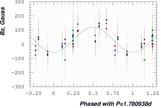
Figure 2: The same as in Fig. 1 but excluding the measurement with the lowest accuracy. The solid line represents a fit to the data with a mean value for the magnetic field of $\overline{\left<B_{\rm z}\right>}=32.3\pm 8.2$ G, an amplitude of $A_{\left<B_{\rm z}\right>}=88.4\pm 15.2$ G, and a root mean square value of 46.7 G.

The longitudinal magnetic field variation of $\zeta$ Pup over a period of 1.78 d is presented in Fig. 1, for absorption and emission lines combined, absorption lines alone, and for hydrogen lines. The solid line represents a fit to the joined three sets of measurements, with a mean value of the magnetic field of $\overline{\left<B_{\rm z}\right>}=28.2\pm 10.5$ G and an amplitude of $A_{\left<B_{\rm z}\right>}=104.0\pm 19.2$ G. For the presented fit, we assume a zero phase corresponding to the negative field extremum at MJD56570.2611. The measurements phased with the period 1.78 d show a single-wave variation. Noteworthy, our phasing of the magnetic field measurements with other periods mentioned in the literature do not display such a sinusoidal variability.

No longitudinal magnetic field measurement shows a 3$\sigma$ detection. The highest significance levels in the measurements were achieved at phase 0.037 (at 2.4$\sigma$) for the measurements using the entire spectral range and at phase 0.668 (at 2.2$\sigma$) for the measurement carried out excluding emission lines. Among the presented measurements, the measurement obtained at phase 0.037 shows the highest field strength, but also the lowest accuracy. As the assigned weights are inversely proportional to the squares of the measurement errors in the fitting procedure, the contribution of this measurement is expected to be by a factor of $\sim$7 lower than that for the other measurements. To check the likelihood of the obtained sinusoidal fit, we repeated the fitting procedure excluding this measurement. The result is presented in Fig. 2, where the solid line shows the fit to the joined three sets of measurements. We obtain a rather similar mean value of the magnetic field $\overline{\left<B_{\rm z}\right>}=32.3\pm 8.2$ G, and a slightly smaller field amplitude $A_{\left<B_{\rm z}\right>}=88.4\pm 15.2$ G. For this fitting model superimposed on the data presented in Fig. 2, we calculate a reduced $\chi^{2}$ of 0.36. The reduced $\chi^{2}$ value calculated assuming a model in which the longitudinal magnetic field is constant and equal to 0, is 0.84. Thus, the zero field assumption also represents the data well. Low $\chi^{2}$ values could point to an overestimation of the errors, which we rule out, or to fitting noise.

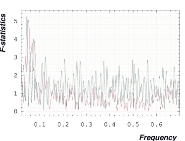
Figure 3: Frequency periodogram (in d^-1) for the longitudinal magnetic field measurements using the entire spectrum. The window function is indicated by the red color.

We note that no periodicity of the magnetic variability is indicated in our frequency periodograms obtained for the magnetic field measurements. The result of the frequency analysis performed using a non-linear least squares fit to the multiple harmonics utilizing the Levenberg-Marquardt method (Press et al., 1992) with an optional possibility of prewhitening the trial harmonics is presented in Fig. 3. To detect the most probable period, we calculated the frequency spectrum and for each trial frequency we performed a statistical F-test of the null hypothesis for the absence of periodicity (Seber, 1977). The resulting F-statistics can be thought of as the total sum including covariances of the ratio of harmonic amplitudes to their standard deviations, i.e. a signal-to-noise ratio.

Table 2: Assumed magnetic field model for $\zeta$ Pup, including the data point at phase 0.037 (left), and excluding it (right).

$\overline{\left<B_{\rm z}\right>}$	[G]	28.2$\pm$	10.5	32.3$\pm$	8.2
$A_{\left<B_{\rm z}\right>}$	[G]	104.0$\pm$	19.2	88.4$\pm$	15.2
$P$	[d]	$1.780938\pm 0.000093$
$R$	[$R_{\odot}$]	$14.0\pm 0.4$
$v_{\rm eq}$	[km s-1]	$398\pm 11$
$v$ sin $i$	[km s-1]	$208\pm 5$
$i$	[∘]	$31.5\pm 1.3$
$\beta$	[∘]	80.6$\pm$	3.9	77.4$\pm$	3.8
$B_{\rm d}$	[G]	681$\pm$	125	585$\pm$	93

If we assume that the magnetic field variability displayed in Figs. 1 and  2 is real, then the observed single-wave variation in the longitudinal magnetic field during the stellar rotation cycle would indicate a dominant dipolar contribution to the magnetic field topology. If the star is an oblique dipole rotator, the magnetic dipole axis tilt $\beta$ is constrained by

$$\frac{\left<B_{\rm z}\right>_{\rm max}}{\left<B_{\rm z}\right>_{\rm min}}=\frac{\cos(i+\beta)}{\cos(i-\beta)},$$ (3)

where the inclination angle $i$ can be derived from considerations of the stellar fundamental parameters (Preston, 1967). Using for the stellar radius $R=14\pm 0.4\,R_{\odot}$ (Schilbach & Röser, 2008) combined with the period of 1.78 d, we obtain $v_{\rm eq}=398\pm 11$ km s^-1. Using $v\,\sin\,i=208\pm 5$ km s^-1 (Conti & Ebbets, 1977) we obtain the inclination angle $i=31.5\pm 1.3^{\circ}$. In Table 2, we show for $\zeta$ Pup the corresponding parameters of the possible magnetic field dipole models. The estimated dipole strengths of $681\pm 125$ G and $585\pm 93$ G are significantly higher than the dipole strength value suggested by David-Uraz et al. (2014), who determined an upper limit of 121 G from one single longitudinal magnetic field measurement. Obviously, greater sensitivity in future magnetic field observations is necessary to further test the presence of a magnetic field in $\zeta$ Pup.

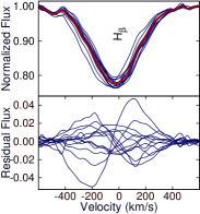
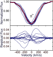
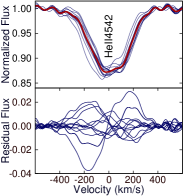
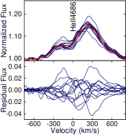
Figure 4: Variability of hydrogen and He ii lines in FORS 2 spectra obtained at thirteen different epochs. The upper panels show overplotted profiles while the lower panels present the differences between individual line profiles and the average profiles. The average profile for each line is highlighted in red.

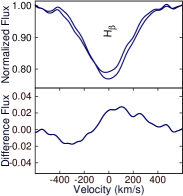
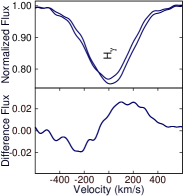
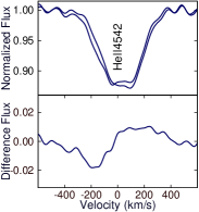
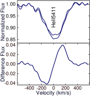
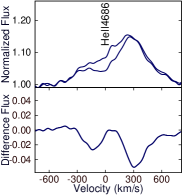
Figure 5: Variability of hydrogen and He ii lines in FORS 2 spectra obtained on the same night within a time interval of 4.4 h. The upper panels show overplotted profiles while the lower panels present the differences between the individual line profiles.

As was already reported in the literature, line profiles belonging to different elements in $\zeta$ Pup show strong variability. As an example, we present in Fig. 4 the overplotted profiles of hydrogen lines H$\beta$ and H$\gamma$ and of the He ii lines 4542, 5411, and 4686 and the differences between individual line profiles and the average profiles. The largest variability amplitude in the velocity frame and in the line profile depths is detected in hydrogen lines and in the He ii 4686 line. The He ii 4686 line shows the presence of two components, where the blue component becomes stronger in the vicinity of the positive magnetic extremum and slightly stronger again in the vicinity of the negative field extremum. Similar to the results of Baade (1986), who used the C iv 5801, 5812 lines, the He ii 4542 line exhibits a clear splitting at certain epochs, while the line He ii 5411 displays a moderate splitting. Although we detect that the intensity of the split components in the He ii 4542 line changes with time, more observations are necessary to assess the character of this variability. Baade (1986) interpreted the detected variations as non-radial oscillations with a period of about 0.356 d. A rather strong spectral variability is also detected on a short time scale: two FORS 2 observations of $\zeta$ Pup were obtained on the same night on 2013 December 21 within a time interval of only of 4.4 h. In Fig.5, we present for the same lines as in Fig. 4 the differences between the observations obtained within the same night.

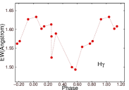
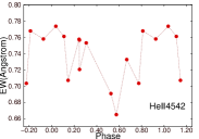
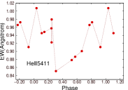
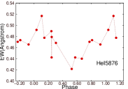
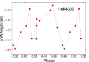
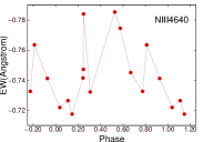
Figure 6: Variability of equivalent widths of lines belonging to different elements over the period of 1.78 d. The measurement accuracy corresponds to the size of the plotted symbols.

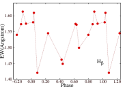
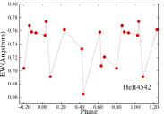
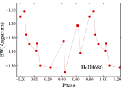
Figure 7: Variation of equivalent widths phased with a period of 5.26 d of the lines H$\beta$, He ii 4542, and He ii 4686.

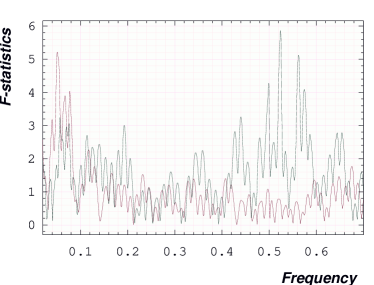
Figure 8: Frequency periodogram (in d^-1) for the equivalent width measurements for the H$\beta$ line. The window function is indicated by the red color.

It is intriguing that the presence of a period of 1.78 d is indicated in the variability of equivalent widths of lines belonging to different elements. In Fig. 6, we present their variations over the period of 1.78 d. Clear variability is detected for all studied absorption lines. The equivalent widths of absorption hydrogen and helium lines decreases in the vicinity of the positive magnetic pole, while the intensity of the emission lines He ii 4686 and the blend of N iii lines at $\sim$4640 Å behave opposite, showing an increase at the positive magnetic pole. However, as is presented in Fig. 7, no smooth variation of equivalent widths over a longer period (we use in these plots the period of 5.26 d suggested by Balona 1992) is detected. Our frequency periodogram obtained for equivalent width measurements of H$\beta$ is presented in Fig. 8. The second largest peak in this periodogram is close to 0.56 d^-1 (equivalent to a period of 1.78 d) while the largest peak corresponds to a period of about 1.91 d. Interestingly, a smaller peak is found close to 0.192 d^-1, corresponding to a period of about 5.21 d.

Further, our study of the temporal behaviour of different lines shows a shift in the line position at phases between 0.80 and 0.90 by about 60 km s^-1 where the change from positive to negative polarity of the longitudinal magnetic field takes place. No such strong shift is detected at the phase when the field changes the polarity from negative to positive. The He ii 4686 line shows the presence of two components, where the blue component becomes stronger in the vicinity of the positive magnetic extremum and slightly stronger again in the vicinity of the negative field extremum. The He ii 4542 line shows some kind of double-peak structure, where the intensity of each absorption peak changes with time. However, more spectra are needed to understand the character of the variability in more detail. Noteworthy, similar double-peak structures are observed in the shapes of He lines in the spectra of the Of?p star CPD $-28^{\circ}$ 2561 (Hubrig et al., 2015a) and the Wolf-Rayet star WR 6 (Hubrig et al., submitted to MNRAS).

4 Discussion

No magnetic field is detected in $\zeta$ Pup, as no magnetic field measurement has a significance level higher than 2.4$\sigma$. However, we cannot exclude a possible single-wave variation of the longitudinal magnetic field measurements. The period of 1.78 d detected by Howarth & Stevens (2014) appears convincing and significant, and was also confirmed by BRITE observations (Ramiaramanantsoa, priv. comm.). However, Howarth & Stevens (2014) proposed that this period may be explained by stellar pulsations, while our data suggest that the period may be explained by stellar rotation. It is important to confirm this suggestion, using more extensive spectroscopic material.

Our work indicates that spectroscopic/spectropolarimetric studies appear most suitable for the determination of rotation periods. For instance, X-rays from massive stars, although present, are not well understood. The search of periodical modulation in X-ray observations of $\zeta$ Pup has a long history, but no conclusive detection was presented in any study yet. Berghoefer et al. (1996) used ROSAT to monitor $\zeta$ Puppis over eleven days, totaling 56 ks of observing time. Simultaneously with the X-ray observations, the variability in the H$\alpha$ line was also monitored. The authors reported a 16.667 h modulation both in the H$\alpha$ line as well as in the X-ray band pass between 0.9 and 2.0 keV. However, this periodicity was not confirmed by Oskinova, Clarke, & Pollock (2001) and Nazé, Oskinova, & Gosset (2013), who used extensive ASCA and XMM-Newton observations. Instead, some modulations with an amplitude of $\sim 15$% on a time scale longer than 1 d were found, but these did not show coherent, systematic periodicity.

Summarizing, our search for the presence of a magnetic field in the fast rotating runaway stars $\zeta$ Oph and $\zeta$ Pup did not result in any significant detection. Admittedly, a major part of the magnetic massive stars rotate rather slow, but still a small group of early B-type stars with strong magnetic fields and extraordinary fast rotation exists, posing a mystery for theories of star formation and magnetic field evolution (e.g.  Rivinius et al. 2010; Hubrig et al. 2015b). The origin of magnetic fields in massive stars is still under debate. It was suggested that the fields are either “fossil” remnants of the Galactic ISM field, which is amplified during the collapse of a magnetised gas cloud (e.g. Price & Bate 2007), or that they are formed in a dramatic close binary interaction, i.e., in a merger of two stars or a dynamical mass transfer event (e.g. Ferrario et al. 2009). Tetzlaff, Neuhäuser, & Hohle (2010) reinvestigated the scenario of a binary SN in Upper Scorpius involving $\zeta$ Oph and PSR B1929+10 and concluded that it is very likely that both objects were ejected during the same supernova event. Although in the case of $\zeta$ Oph binary interaction is expected, no significant field was detected in this star. On the other hand, the results of our previous studies seem to indicate that the presence of a magnetic field is more frequently detected in candidate runaway stars than in stars belonging to clusters or associations (e.g. Hubrig, Kharchenko, & Schöller 2011). Since the number of detected magnetic O-type stars is still rather small, these results need to be confirmed with a larger sample in the future.

References

- Angel & Landstreet (1970) Angel J. R. P., & Landstreet J. D. 1970, ApJ, 160, L147
- Appenzeller et al. (1998) Appenzeller, I., Fricke, W., Fürtig, W., et al. 1998, The ESO Messenger, 94, 1
- Baade (1986) Baade, D. 1986, in: NATO Advanced Science Institutes (ASI) Series C, D. O. Gough, ed., 169, 465
- Balona (1992) Balona, L. A. 1992, MNRAS, 254, 404
- Bagnulo et al. (2012) Bagnulo, S., Landstreet, J. D., Fossati, L., et al. 2012, A&A, 538, A129
- Berghoefer et al. (1996) Berghoefer, T. W., Baade, D., Schmitt, J. H. M. M., et al. 1996, A&A, 306, 899
- Cantiello et al. (2009) Cantiello M., Langer, N., Brott, I., et al. 2009, A&A, 499, 279
- Chesneau & Moffat (2002) Chesneau, O.,& Moffat, A. F. J. 2002, PASP, 114, 612
- Conti & Leep (1974) Conti, P. S., & Leep, E. M. 1974, ApJ, 193, 113
- Conti & Ebbets (1977) Conti, P. S., & Ebbets, D. 1977, ApJ, 213, 438
- David-Uraz et al. (2014) David-Uraz, A., Wade, G. A., Petit, V., et al. 2014, MNRAS, 444, 429
- Eversberg et al. (1998) Eversberg, T., Lépine, S., & Moffat, A. F. 1998, ApJ, 494, 799
- Ferrario et al. (2009) Ferrario, L., Pringle, J. E, Tout, C. A, & Wickramasinghe, D. T. 2009, MNRAS, 400, L7
- Harries (2000) Harries, T. J. 2000, MNRAS, 315, 722
- Harries, Howarth, & Evans (2002) Harries, T. J., Howarth, I. D., & Evans, C. J. 2002, MNRAS, 337, 341
- Hoogerwerf, de Bruijne, & de Zeeuw (2001) Hoogerwerf, R., de Bruijne, J. H. J., & de Zeeuw, P. T. 2001, A&A, 365, 49
- Howarth & Stevens (2014) Howarth, I. D., & Stevens, I. R. 2014, MNRAS, 445, 2878
- Hubrig et al. (2004a) Hubrig, S., Kurtz, D. W., Bagnulo, S., et al. 2004a, A&A, 415, 661
- Hubrig et al. (2004b) Hubrig, S., Szeifert, T., Schöller, M., et al. 2004b, A&A, 415, 685
- Hubrig et al. (2006) Hubrig, S., Briquet, M., Schöller, M., et al. 2006, MNRAS, 369, L61
- Hubrig et al. (2008) Hubrig, S., Schöller, M., Schnerr, R. S., et al. 2008, A&A, 490, 793
- Hubrig et al. (2009) Hubrig, S., Briquet, M., De Cat, P., et al. 2009, Astr. Nachr., 330, 317
- Hubrig, Oskinova, & Schöller (2011) Hubrig, S., Oskinova, L. M., & Schöller, M. 2011, Astr. Nachr., 332, 147
- Hubrig et al. (2011) Hubrig, S., Schöller, M., Kharchenko, N. V., et al. 2011, A&A, 528, A151
- Hubrig, Kharchenko, & Schöller (2011) Hubrig, S., Kharchenko, N. V., & Schöller, M. 2011c, Astr. Nachr., 332, 65
- Hubrig et al. (2013) Hubrig, S., Schöller, M., Ilyin, I., et al. 2013, A&A, 551, A33
- Hubrig, Schöller, & Kholtygin (2014) Hubrig, S., Schöller, M., & Kholtygin, A. F. 2014, MNRAS, 440, L6
- Hubrig et al. (2015a) Hubrig, S., Schöller, M., Kholtygin, A. F., et al. 2015a, MNRAS, 447, 1885
- Hubrig et al. (2015b) Hubrig, S., Schöller, M., Fossati, L., et al. 2015b, A&A, 578, L3
- Hubrig et al. (2016) Hubrig, S., Schöller, M., Kholtygin, A. F., et al. 2016, in “Radiation mechanisms of astrophysical objects: classics today”, Proc. of the conference held in St. Petersburg, Russia, 2015 Sep 21-25; also arxiv.org:1602.08930
- Kambe, Ando, & Hirata (1993) Kambe, E., Ando, H., & Hirata, R. 1993, A&A, 273, 435
- Moffat & Michaud (1981) Moffat, A. F. J., & Michaud, G. 1981, ApJ, 251, 133
- Nazé, Oskinova, & Gosset (2013) Nazé, Y., Oskinova, L. M., & Gosset, E. 2013, ApJ, 763, 143
- Oskinova, Clarke, & Pollock (2001) Oskinova, L. M., Clarke, D., & Pollock, A. M. T. 2001, A&A, 378, 21
- Pollmann (2012) Pollmann, E. 2012, IBVS, 6034, 1
- Press et al. (1992) Press, W. H., Teukolsky, S. A., Vetterling, W. T., & Flannery, B. P. 1992, Numerical Recipes, 2nd edn. (Cambridge: Cambridge University Press)
- Preston (1967) Preston, G. W. 1967, ApJ, 150, 547
- Price & Bate (2007) Price, D. J., & Bate, M. R. 2007, MNRAS, 377, 77
- Reid & Howarth (1996) Reid, A. H. N., & Howarth, I. D. 1996, A&A, 311, 616
- Ramiaramanantsoa et al. (2014) Ramiaramanantsoa T., Moffat, A. F. J., Chené, A.-N., et al. 2014, MNRAS, 441, 910
- Rivinius et al. (2010) Rivinius, Th., Szeifert, Th., Barrera, L., et al. 2010, MNRAS, 405, L46
- Rivinius et al. (2013) Rivinius, T., Townsend, R. H. D., & Kochukhov, O. et al. 2013, MNRAS, 429, 177,
- Schilbach & Röser (2008) Schilbach, E., & Röser, S. 2008, A&A, 489, 105
- Seber (1977) Seber, G. A. F. 1977, Linear Regression Analysis (New York: Wiley)
- Tetzlaff, Neuhäuser, & Hohle (2010) Tetzlaff, N., Neuhäuser, R., & Hohle, M. M. 2010, MNRAS, 402, 2369
- Vink et al. (2009) Vink, J. S., Davies, B., Harries, T. J., et al. 2009, A&A, 505, 743
- Waldron & Cassinelli (2007) Waldron W. L., & Cassinelli J. P. 2007, ApJ, 668, 456