Capacity Achieving Distributions & Information Lossless Randomized Strategies for Feedback Channels with Memory: The LQG Theory of Directed Information-Part II

Abstract

A methodology is developed to realized optimal channel input conditional distributions, which maximize the finite-time horizon directed information, for channels with memory and feedback, by information lossless randomized strategies. The methodology is applied to general Time-Varying Multiple Input Multiple Output (MIMO) Gaussian Linear Channel Models (G-LCMs) with memory, subject to average transmission cost constraints of quadratic form. The realizations of optimal distributions by randomized strategies are shown to exhibit a decomposion into a deterministic part and a random part. The decomposition reveals the dual role of randomized strategies, to control the channel output process and to transmit new information over the channels. Moreover, a separation principle is shown between the computation of the optimal deterministic part and the random part of the randomized strategies. The dual role of randomized strategies generalizes the Linear-Quadratic-Gaussian (LQG) stochastic optimal control theory to directed information pay-offs.

The characterizations of feedback capacity are obtained from the per unit time limits of finite-time horizon directed information, without imposing á priori assumptions, such as, stability of channel models or ergodicity of channel input and output processes. For time-invariant MIMO G-LCMs with memory, it is shown that whether feedback increases capacity, is directly related to the channel parameters and the transmission cost function, through the solutions of Riccati matrix equations, and moreover for unstable channels, feedback capacity is non-zero, provided the power exceeds a critical level.

I Introduction

Stochastic optimal control theory and a variational equality of directed information are applied in [1], to identify the information structures of optimal channel input conditional distributions, ${\cal P}_{[0,n]}\stackrel{{\scriptstyle\triangle}}{{=}}\big{\{}{\bf P}_{A_{i}|A^{i-1},B^{i-1}}:i=0,1,\ldots,n\big{\}}\subset{\cal P}_{[0,n]}(\kappa)$, which maximize the finite-time horizon directed information $I(A^{n}\rightarrow B^{n})$, for channels with memory and feedback, defined by

$$C_{A^{n}\rightarrow B^{n}}^{FB}(\kappa)=\sup_{{\cal P}_{[0,n]}(\kappa)}I(A^{n}\rightarrow B^{n}),\hskip 14.45377pt\hskip 14.45377ptI(A^{n}\rightarrow B^{n})\stackrel{{\scriptstyle\triangle}}{{=}}\sum_{i=0}^{n}I(A^{i};B_{i}|B^{i-1})$$ (I.1)

where $A^{n}\stackrel{{\scriptstyle\triangle}}{{=}}\{A_{0},A_{1},\ldots,A_{n}\}$ and $B^{n}\stackrel{{\scriptstyle\triangle}}{{=}}\{B_{0},B_{1},\ldots,B_{n}\}$, are channel input and output RVs, respectively, and ${\cal P}_{[0,n]}(\kappa)\subset{\cal P}_{[0,n]}$ denotes a subset of distributions, which satisfy a transmission cost constraint and $\kappa$ is the power. Specifically, given a channel distribution and a transmission cost constraint, the optimal channel input conditional distributions, which maximize $I(A^{n}\rightarrow B^{n})$, are characterized by conditional independence properties, called the “information structures”. The information structures of optimal distributions simplify the resulting finite-time horizon optimization problem called the “characterization of Finite Transmission Feedback Information (FTFI) capacity”. In principle, the information structures of optimal distributions and corresponding characterizations of FTFI capacity, are analogous to those of memoryless channels without feedback, which are established via the well-known upper bounds

$$C_{A^{n};B^{n}}\stackrel{{\scriptstyle\triangle}}{{=}}\max_{{\bf P}_{A^{n}}}I(A^{n};B^{n})\leq\max_{{\bf P}_{A_{i}}:i=0,\ldots,n}\sum_{i=0}^{n}I(A_{i};B_{i})\leq(n+1)\max_{{\bf P}_{A}}I(A;B)\equiv(n+1)C$$ (I.2)

which are achievable if ${\bf P}_{A_{i}|A^{i-1}}={\bf P}_{A_{i}},i=0,\ldots,n$ and identically distributed, which implies the joint process $\{(A_{i},B_{i}):i=0,\ldots,n\}$ is identically distributed, and hence ergodic. For memoryless channels with feedback, (I.2) remains valid, provided it is shown, via the converse to the coding theorem, that feedback does not give better upper bounds [2]. For memoryless channels the above bounds are applied in the converse part of the coding theorem, to obtain a tight bound on any achievable rate, while for the direct part, codes are generated independently according to ${\bf P}_{A^{n}}^{*}(da^{n})\stackrel{{\scriptstyle\triangle}}{{=}}\otimes_{i=0}^{n}{\bf P}_{A}^{*}(da_{i})$, where ${\bf P}_{A}^{*}$ is the one which corresponds to $C$.
However, to make the transition from memoryless channels to channels with memory, without any á priori assumptions, such as, stationarity, ergodicity or information stability, it is necessary to investigate the characterizations of FTFI capacity $C_{A^{n}\rightarrow B^{n}}^{FB}(\kappa)$, and its asymptotic properties via the per unit time limiting versions

$$C_{A^{\infty}\rightarrow B^{\infty}}^{FB}(\kappa)\stackrel{{\scriptstyle\triangle}}{{=}}\liminf_{n\longrightarrow\infty}\frac{1}{n+1}C_{A^{n}\rightarrow B^{n}}^{FB}(\kappa)$$ (I.3)

Specifically, it is illustrated in this paper that
1) the information structures of optimal channel input distributions and corresponding characterizations of FTFI capacity, translate into corresponding information structures for $C_{A^{\infty}\rightarrow B^{\infty}}^{FB}(\kappa)$, and moreover via the converse coding theorem, tight bounds on any achievable code rate (of feedback codes) can be obtained, while the direct part of the coding theorem can be investigated, without unnecessary á priori assumptions on the channel, such as, stationarity, ergodicity, or information stability of the joint process $\{(A_{i},B_{i}):i=0,1,\ldots\}$;
2) the characterizations of the FTFI capacity reveal several hidden properties of the role of feedback to affect the channel output process, including fundamental properties of optimal channel input conditional distributions, which achieve $C_{A^{\infty}\rightarrow B^{\infty}}^{FB}(\kappa)$, and properties of channel parameters so that $C_{A^{\infty}\rightarrow B^{\infty}}^{FB}(\kappa)$ corresponds to feedback capacity.

Application examples are developed to unfold the role of feedback, in communication systems with memory.

I-A Contributions

The main contributions of this second part of the two part investigation, are the following.

i)

Develop a methodology to realize optimal channel input conditional distributions, by information lossless (one-to-one and onto maps) randomized strategies (deterministic functions) driven by uniform Random Variables (RVs), and to derive alternative equivalent characterizations of FTFI capacity. In specific application examples, such as, Gaussian channels with memory, in which the capacity achieving optimal channel input conditional distributions are Gaussian, the uniform RVs transform the randomized strategies into capacity achieving randomized strategies, driven by Gaussian random processes;

ii)

identify a dual role (and hidden features) of optimal channel input conditional distributions and information lossless randomized strategies, to control the channel output process, and to transmit new information over the channels, while they achieve the characterizations of FTFI capacity and feedback capacity;

iii)

identify sufficient conditions, in terms of channel parameters, which define the channel conditional distributions and transmission cost functions (if constraints are imposed on the channel input conditional distributions), for the quantity $C_{A^{\infty}\rightarrow B^{\infty}}^{FB}(\kappa)$ to correspond to feedback capacity.

The channel conditional distributions considered in this paper, are either one of the following two classes.

$$\mbox{Channel Distributions Class A.}\hskip 7.22743pt{\bf P}_{B_{i}|B^{i-1},A^{i}}(db_{i}|b^{i-1},a^{i})={\bf P}_{B_{i}|B^{i-1},A_{i}}(db_{i}|b^{i-1},a_{i}),$$ (I.4)

$$\mbox{Channel Distributions Class B.}\hskip 7.22743pt{\bf P}_{B_{i}|B^{i-1},A^{i}}(db_{i}|b^{i-1},a^{i})={\bf P}_{B_{i}|B_{i-M}^{i-1},A_{i}}(db_{i}|b_{i-M}^{i-1},a_{i}),\hskip 7.22743pti=0,\ldots,n$$ (I.5)

where $M$ is a nonnegative integer. The convention for $M=0$, is ${\bf P}_{B_{i}|B_{i-M}^{i-1},A_{i}}(db_{i}|b_{i-M}^{i-1},a_{i})={\bf P}_{B_{i}|A_{i}}(db_{i}|a_{i}),\hskip 7.22743pti=0,1,\ldots,n$, that is, the channel degenerates to a memoryless channel.
The average transmission cost constraint is of the form

$${\cal P}_{[0,n]}(\kappa)\stackrel{{\scriptstyle\triangle}}{{=}} \Big{\{}{\bf P}_{A_{i}|A^{i-1},B^{i-1}},i=0,\ldots,n:\frac{1}{n+1}{\bf E}\Big{(}\sum_{i=0}^{n}\gamma_{i}(T^{i}A^{n},T^{i}B^{n})\Big{)}\leq\kappa\Big{\}}$$ (I.6)

where the transmission cost functions are either one of the following two classes

$$\mbox{Transmission Cost Functions Class A.}\hskip 7.22743pt\gamma_{i}(T^{i}a^{n},T^{i}b^{n})={\gamma}_{i}^{A}(a_{i},b^{i}),$$ (I.7)

$$\mbox{Transmission Cost Functions Class B.}\hskip 7.22743pt\gamma_{i}(T^{i}a^{n},T^{i}b^{n})={\gamma}_{i}^{B}(a_{i},b_{i-K}^{i}),\hskip 14.45377pti=0,\ldots,n.$$ (I.8)

where $K$ is nonegative and finite.
In this paper, the dual role of optimal channel input distributions and randomized strategies, are only illustrated for Multiple-Input Multiple Output (MIMO) Gaussian Linear Channel Models (G-LCMs) with memory, via a provocative direct connection to the Linear-Quadratic-Gaussian (LQG) stochastic optimal control theory, stability of linear stochastic controlled systems, and Lyapunov and Riccati matrix equations. Indeed, the LQG stochastic optimal control theory generalizes in a natural way to directed information pey-off functionals. For the readers convenience a short summary of these concepts is given in Appendix -D. These tools are necessary to to treat processes $\{(A_{i},B_{i}):i=0,1,\ldots,\}$, which are not assumed á priori to be stationary, ergodic or information stable. Rather, it is shown via these mathematical concepts that the optimal channel input conditional distribution induces asymptotic ergodicity of the joint process $\{(A_{i},B_{i}):i=0,1,\ldots\}$.
For these application examples, it is further shown that the optimal randomized strategies, which achieve FTFI capacity decompose into a deterministic part and a random part. Through this decomposition, a separation principle is shown, between the role of randomized strategies to control the channel output process and to transmit new information over the channel. It is also shown that the deterministic part corresponds to the optimal solution of the LQG stochastic optimal control problem, while the random part is determined from water-filling type equations. There is however, a fundamental difference; in LQG stochastic optimal control theory, randomized strategies do not incur a better performance than deterministic strategies.

One of the important conclusions of this paper, is that if the channel input process is the control process, the channel output is the controlled process, the pay-off of LQG stochastic optimal control theory [3] is replaced by the directed information from the control process to the controlled process, then randomized control strategies have an operation meaning in terms of conveying information from the control process to the controlled process, and exhibit all properties of LQG theory.
In Section I-C, a short summary of the main concepts, methods, and results obtained in this paper are presented.

I-B Literature Review

Cover and Pombra [4] investigated the non-stationary non-ergodic Additive Gaussian Noise (AGN) channel with memory, defined by

$$B_{i}=A_{i}+V_{i},\hskip 14.45377pti=0,1,\ldots,n,\hskip 14.45377pt\frac{1}{n+1}\sum_{i=0}^{n}{\bf E}\big{\{}|A_{i}|^{2}\big{\}}\leq\kappa,\hskip 7.22743pt\kappa\in[0,\infty)$$ (I.9)

where $\{V_{i}:i=0,1,\ldots,n\}$ is a real-valued (scalar) jointly non-stationary Gaussian process, with covariance $K_{V^{n}}$, and “$A^{n}$ is causally related to $V^{n}$” . The authors in [4], applied the maximizing entropy property of Gaussian distributions (and converse coding arguments) to characterize feedback capacity $C_{W;B^{\infty}}^{FB,CP}(\kappa)\stackrel{{\scriptstyle\triangle}}{{=}}\lim_{n\longrightarrow\infty}\frac{1}{n+1}C_{W;B^{n}}^{FB,CP}(\kappa)$, via the following characterization of FTFI capacity.

$$C_{W;B^{n}}^{FB,CP}(\kappa)=\max_{\Big{\{}(\overline{\Gamma}^{n},K_{\overline{Z}^{n}}):\frac{1}{n+1}{\bf E}\big{\{}tr\big{(}A^{n}(A^{n})^{T}\big{)}\big{\}}\leq\kappa,\hskip 7.22743ptA^{n}=\overline{\Gamma}^{n}V^{n}+\overline{Z}^{n}\Big{\}}}H(B^{n})-H(V^{n})$$ (I.10)

where $\overline{Z}^{n}\stackrel{{\scriptstyle\triangle}}{{=}}\{\overline{Z}_{i}:i=0,1,\ldots,n\}$ is a correlated Gaussian process $N({0},K_{\overline{Z}^{n}})$, orthogonal to $V^{n}\stackrel{{\scriptstyle\triangle}}{{=}}\{V_{i}:i=0,\ldots,n\}$, and $\overline{\Gamma}^{n}$ is lower diagonal time-varying matrix with deterministic entries (i.e., $A_{i}=\sum_{j=0}^{i-1}\overline{\gamma}_{i,j}V_{j}+\overline{Z}_{i},i=0,\ldots,n$). Although, the authors in [4] call $\{\overline{Z}_{i}:i=0,\ldots,n\}$ an innovations like process, this is not to be confused with the standard definition of an Innovations Process, which is an orthogonal process. Yang Kavcic and Tatikonda [5] considered stationary AGN channels with memory, including the Cover and Pombra AGN channel, and applied dynamic programming as a means of computing optimal channel input conditional distributions, which maximize directed information. Kim [6] investigated the stationary version of the Cover and Pombra AGN channel, under the assumption that the noise power spectral density corresponds to a stationary Gaussian autoregressive moving-average model of order $K$, among other things. The AGN channel with memory investigated in [4, 6], dates back to early investigations by Butman [7, 8].
Recently, feedback capacity problems for finite alphabet channels, without transmission cost constraints, are investigated, for the trapdoor channel by Permuter, Cuff, Van Roy and Tsachy [9], for the the Ising Channel by Elishco and Permuter [10], for the the Post$(a,b)$ channel by Permuter, Asnani and Tsachy [11], for channels in which the input to the channel and the channel state are related by a one-to-one mapping by Tatikonda, Yang and Kavcic [12], and for the Unit Memory Channel Output (UMCO) channel (i.e., $\big{\{}{\bf P}_{B_{i}|B_{i-1},A_{i}}:i=0,\ldots,n\}$) by Chen and Berger [13] (under the assumption the optimal channel input distribution is $\big{\{}{\bf P}_{A_{i}|B_{i-1}}:i=0,\ldots,n\big{\}}$). In [14], the BSSC($\alpha,\beta)$ is investigated, with and without feedback and transmission cost. Coding theorems for channels with memory with and without feedback, are developed extensively over the years, for example, in [15, 16, 17, 18, 2, 19, 20, 21, 22, 23, 24, 25, 26, 27].

I-C Discussion of Methodology and Main Results

The methodology and results listed under i)-iii) (and discussion under 1), 2)), are obtained by applying the analogy to stochastic optimal control theory depicted in Fig. I.1, which states the following. The information measure $I(A^{n}\rightarrow B^{n})$ is the pay-off, the channel output process $\{B_{i}:i=0,1,\ldots,n\}$ is the controlled process, and the channel input process $\{A_{i}:i=0,1,\ldots,n\}$ is the control process.

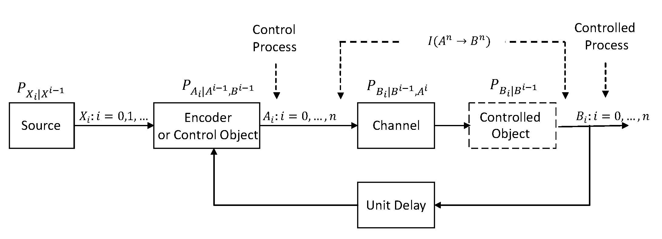
Figure I.1: Communication block diagram and its analogy to stochastic optimal control.

The main results of the paper are summarized and discussed below.

I-C1 Information Lossless Randomized Strategies and Characterizations of FTFI capacity

Section III, describes the methodology applied in i), to derive alternative equivalent characterizations of FTFI capacity, by realizing optimal channel input conditional distributions, which maximize directed information, using randomized strategies, driven by uniform Random Variables.
An alternative equivalent characterization of FTFI capacity is illustrated below.

Equivalent Characterizations of FTFI Capacity for Class B channels and transmission cost functions. Consider $\Big{\{}{\bf P}_{A_{i}|B_{i-M}^{i-1}},\gamma_{i}(T^{i}a^{n},T^{i}b^{n})=\gamma_{i}^{B}(a_{i},b_{i-M}^{i-1}):i=0,\ldots,n\Big{\}}$, $M\geq 1$. In [1], it is shown that the maximization of $I(A^{n}\rightarrow B^{n})$ over all distributions ${\bf P}_{A_{i}|A^{i-1},B^{i-1}}:i=0,\ldots,n\}$, which satisfy the constraint $\frac{1}{n+1}{\bf E}\big{\{}{\gamma}_{i}^{B}(A_{i},B_{i-M}^{i-1})\big{\}}\leq\kappa$, satisfy conditional independence

$${\bf P}_{A_{i}|A^{i-1},B^{i-1}}={\bf P}_{A_{i}|B_{i-M}^{i-1}},\hskip 7.22743pti=0,\ldots,n$$ (I.11)

which implies the information structure of the optimal channel input distribution is $B_{i-M}^{i-1}$ for $i=0,1,\ldots,n$ and the corresponding

joint process $$\big{\{}(A_{i},B_{i}):i=0,\ldots,n\big{\}} \big{\{}B_{i}:i=0,\ldots,n\big{\}} M-$$ and output process are order Markov (I.12)

and the characterization of the FTFI capacity is given by the following expression.

$${C}_{A^{n}\rightarrow B^{n}}^{FB,B.M}(\kappa)=\sup_{{\bf P}_{A_{i}|B_{i-M}^{i-1}},i=0,\ldots,n:\frac{1}{n+1}\sum_{i=0}^{n}{\bf E}\big{\{}{\gamma}_{i}^{B}(A_{i},B_{i-M}^{i-1})\big{\}}\leq\kappa}\sum_{i=0}^{n}{\bf E}\Big{\{}\log\Big{(}\frac{d{\bf P}_{B_{i}|B_{i-M}^{i-1},A_{i}}(\cdot|B_{i-M}^{i-1},A_{i})}{d{\bf P}_{B_{i}|B_{i-M}^{i-1}}(\cdot|B_{i-M}^{i-1})}(B_{i})\Big{)}\Big{\}}.$$ (I.13)

In Theorem III.2, by utilizing the characterization of FTFI capacity (I.13), the following are shown.
(i) The class of optimal channel input distributions satisfying the average transmission cost constraint, are realized by information lossless randomized strategies defined by

$${\cal E}_{[0,n]}^{IL-B.M}(\kappa)\stackrel{{\scriptstyle\triangle}}{{=}}\Big{\{}e_{i}:{\mathbb{B}}_{i-M}^{i-1}\times[0,1]\longmapsto{\mathbb{A}}_{i},\;a_{i}=e_{i}(b_{i-M}^{i-1},u_{i}),\;i=0,\ldots,n:\hskip 7.22743pt\mbox{for a fixed $b_{i-M}^{i-1}$ the map }\;\>$$

$$e_{i}(b_{i-M}^{i-1},\cdot)\hskip 7.22743pt\mbox{is one-to-one and onto ${\mathbb{A}}_{i},$ for $i=0,\ldots,n$},\hskip 7.22743pt\frac{1}{n+1}\sum_{i=0}^{n}{\bf E}^{e}\Big{(}\gamma_{i}^{B}(e_{i}(B_{i-M}^{i-1},U_{i}),B_{i-M}^{i-1})\Big{)}\leq\kappa\Big{\}}$$ (I.14)

where $\big{\{}U_{i}:i=0,\ldots,n\big{\}}$ are uniform RVs.
(ii) An alternative equivalent characterization of the FTFI capacity (I.13), is given by

$${C}_{A^{n}\rightarrow B^{n}}^{FB,B.M}(\kappa)= \sup_{\big{\{}e_{i}(\cdot,\cdot):i=0,\ldots,n\big{\}}\in{\cal E}_{0,n}^{IL-B.M}(\kappa)}\sum_{i=0}^{n}{\bf E}^{e}\Big{\{}\log\Big{(}\frac{{\bf P}(\cdot|B_{i-M}^{i-1},e_{i}(B_{i-M}^{i-1},U_{i}))}{{\bf P}^{e}(\cdot|B_{i-M}^{i-1})}(B_{i})\Big{)}\Big{\}}$$ (I.15)

$$\equiv \sup_{\big{\{}e_{i}(b_{i-M}^{i-1},u_{i}):i=0,\ldots,n\big{\}}\in{\cal E}_{[0,n]}^{IL-B.M}}\sum_{i=0}^{n}I^{e}(U_{i};B_{i}|B_{i-M}^{i-1})$$ (I.16)

where the channel output transition probabilities are given by

$${\bf P}^{e}(db_{i}|b_{i-M}^{i-1})=\int_{{\mathbb{U}}_{i}}{\bf P}(dB_{i}|B_{i-M}^{i-1},e_{i}(b_{i-M}^{i-1},u_{i})){\bf P}_{U_{i}}(du_{i}),\hskip 7.22743pti=0,1,\ldots,n.$$ (I.17)

In application examples, the maximizing strategy, $\big{\{}e_{i}^{*}(\cdot,\cdot):i=0,\ldots,n\big{\}}\in{\cal E}_{[0,n]}^{IL-B.M}(\kappa)$, is transformed to $e_{i}^{*}(b_{i-M}^{i-1},\cdot)=\overline{e}_{i}^{*}(b_{i-M}^{i-1},g_{i}(\cdot)),g_{i}:[0,1]\longmapsto{\mathbb{Z}}_{i},z_{i}=g_{i}(u_{i})$, where $\big{\{}Z_{i}=g_{i}(U_{i}):i=0,\ldots,n\big{\}}$ is a specific random process, which induces the maximizing channel input conditional distribution of the characterization of FTFI capacity (I.13).
Further, the following are illustrated, via application examples of Multiple-Input Multiple-Output (MIMO) Gaussian-Linear Channel Models (G-LCM).

I-C2 Dual Role of Randomized Information Lossless Strategies & LQG Theory.

By utilizing (I.15), it is shown that, in general, information lossless randomized strategies have a Dual Role, specifically, to

(a)

optimally control the channel output process $\{B_{i}:i=0,1,\ldots,n\}$, and to

(b)

communicate information optimally, by ensuring no information loss incurs, when randomized strategies are used to realize optimal channel input distributions.

In Theorem IV.2 (Section IV-E)), the dual role of information lossless randomized strategies (and several properties), are illustrated for MIMO Time-Varying Gaussian Linear Channel Models G-LCMs with memory. The following application example illustrates this dual role.
Alternative Characterization of FTFI Capacity for G-LCM-B.1 and The LQG Theory. Consider the MIMO G-LCM-B.1, corresponding to channel Class B and transmission cost Class B, defined by

$$B_{i}=C_{i,i-1}\;B_{i-1}+D_{i,i}\;A_{i}+V_{i},\hskip 7.22743ptB_{-1}=b_{-1},\hskip 7.22743pti=0,\ldots,n,$$ (I.18)

$$\frac{1}{n+1}\sum_{i=0}^{n}{\bf E}\Big{\{}\langle A_{i},R_{i}A_{i}\rangle+\langle B_{i-1},Q_{i,i-1}B_{i-1}\rangle\Big{\}}\leq\kappa,$$ (I.19)

$${\bf P}_{V_{i}|V^{i-1},A^{i}}(dv_{i}|v^{i-1},a^{i})={\bf P}_{V_{i}}(dv_{i}),\hskip 7.22743ptV_{i}\sim N(0,K_{V_{i}}),\hskip 7.22743pti=0,\ldots,n,$$ (I.20)

$$(C_{i,i-1},D_{i,i})\in{\mathbb{R}}^{p\times p}\times{\mathbb{R}}^{p\times q},\;(R_{i},Q_{i,i-1})\in{\mathbb{R}}^{q\times q}\times{\mathbb{R}}^{p\times p},\;R_{i}=R_{i}^{T}\succ 0,Q_{i,i-1}=Q_{i,i-1}^{T}\succeq 0,\;i=0,\ldots,n$$ (I.21)

where $\langle\cdot,\cdot\rangle$ denotes inner product of elements of linear spaces.
In Section IV-B, the following are shown (by using (I.15), with $M=1$).
(iii) The optimal conditional channel input conditional distribution is Gaussian of the form $\big{\{}{\bf P}_{A_{i}|B_{i-1}}^{g}(da_{i}|b_{i-1}):i=0,\ldots,n\big{\}}$ and satisfies the average transmission cost constraint, and such distributions are realized by linear and Gaussian information lossless randomized strategies $e(\cdot)\in{\cal E}_{0,n}^{IL-B.1}(\kappa)$, defined by the set

$${\cal E}_{[0,n]}^{IL-B.1}(\kappa)\stackrel{{\scriptstyle\triangle}}{{=}}\Big{\{}A_{i}^{g}=g_{i}^{B.1}(B_{i-1}^{g})+Z_{i}=\Gamma_{i,i-1}B_{i-1}^{g}+Z_{i},\hskip 7.22743ptZ_{i}\perp B^{g,i-1},\;\{Z_{i}:i=0,\ldots,n\}\hskip 7.22743pt\mbox{independent process},$$

$$Z_{i}\sim N(0,K_{{Z}_{i}}),\>K_{Z_{i}}\succeq 0,\hskip 7.22743pti=0,\ldots,n:\frac{1}{n+1}{\bf E}^{g^{B.1}}\Big{\{}\sum_{i=0}^{n}\Big{[}\langle A_{i}^{g},R_{i,i}A_{i}^{g}\rangle+\langle B_{i-1}^{g},Q_{i,i-1}B_{i-1}^{g}\rangle\Big{]}\Big{\}}\leq\kappa\Big{\}}$$ (I.22)

where $\cdot\perp\cdot$ means the processes are independent. Thus, information lossless randomized strategies in ${\cal E}_{[0,n]}^{IL-B.1}(\kappa)$ are decomposed into two orthogonal parts, one of which is an innovations process (i.e., independent process).
(iv) The characterization of FTFI capacity of the MIMO-G-LCM.B.1 is given by the following expression.

$${C}_{A^{n}\rightarrow B^{n}}^{FB,B.1}(\kappa)=\sup_{\big{\{}\big{(}\Gamma_{i,i-1},Z_{i}\big{)},i=0,\ldots,n\big{\}}\in{\cal E}_{[0,n]}^{IL-B.1}(\kappa)}\frac{1}{2}\sum_{i=0}^{n}\ln\frac{|D_{i,i}K_{Z_{i}}D_{i,i}^{T}+K_{V_{i}}|}{|K_{V_{i}}|}.$$ (I.23)

The decomposition

$$A_{i}^{g}=\Gamma_{i,i-1}B_{i-1}^{g}+Z_{i}\equiv g_{i}^{B.1}(B_{i-1}^{g})+Z_{i},\hskip 7.22743pti=0,\ldots,n$$ (I.24)

implies that the feedback function $\{g_{i}^{B.1}\equiv\Gamma_{i,i-1}:i=0,\ldots,n\}$ is the feedback control law or strategy, which controls the output process $\{B_{i}^{g}:i=0,\ldots,n\}$, while the orthogonal innovations process $\{Z_{i}:i=0,\ldots,n\}$ is responsible to convey new information to the output process, both chosen to maximize (I.23).

In Theorem IV.2, this interpretation is utilized to solve the extremum problem (I.23), via its relation to the Linear-Quadratic-Gaussian (LQG) stochastic optimal control theory (with randomized controls). The following are shown.
(v) The characterization of FTFI capacity is given by

$$C_{A^{n}\rightarrow B^{n}}^{FB,B.1}(\kappa)=\inf_{s\geq 0}\Big{\{}-\int_{{\mathbb{R}}^{p}}\langle b_{-1},P(0)b_{-1}\rangle{\bf P}_{B_{-1}}(db_{-1})+r(0)\Big{\}}$$ (I.25)

where $\big{\{}P(i):i=0,\ldots,n\big{\}}$ is a solution of the Riccati difference matrix equation

$$P(i) =C_{i,i-1}^{T}P(i+1)C_{i,i-1}+sQ_{i,i-1}$$

$$-C_{i,i-1}^{T}P(i+1)D_{i,i}\Big{(}D_{i,i}^{T}P(i+1)D_{i,i}+sR_{i,i}\Big{)}^{-1}\Big{(}C_{i,i-1}^{T}P(i+1)D_{i,i}\Big{)}^{T},\hskip 7.22743pti=0,\ldots,n-1,\hskip 7.22743ptP(n)=sQ_{n,n-1}$$ (I.26)

$s\geq 0$ is the Lagrange multiplier associated with the transmission cost constraint, the optimal random part of the strategy $\{K_{Z_{i}}^{*}:i=0,\ldots,n\}$ (covariance of innovations process) is found from a sequential water filing problem

$$r(i)= r(i+1)+\sup_{K_{Z_{i}}\in{\mathbb{S}}_{+}^{q\times q}}\Big{\{}\frac{1}{2}\log\frac{|D_{i,i}K_{Z_{i}}D_{i,i}^{T}+K_{V_{i}}|}{|K_{V_{i}}|}-tr\Big{(}s\;R_{i,i}K_{Z_{i}}\Big{)}-tr\Big{(}P(i+1)\Big{[}D_{i,i}K_{Z_{i}}D_{i,i}^{T}+K_{V_{i}}\Big{]}\Big{)}\Big{\}},\hskip 7.22743pti=0,\ldots,n-1,$$ (I.27)

$$r(n)= \sup_{K_{Z_{n}}\in{\mathbb{S}}_{+}^{q\times q}}\Big{\{}\frac{1}{2}\log\frac{|D_{n,n}K_{Z_{n}}D_{n,n}^{T}+K_{V_{n}}|}{|K_{V_{n}}|}+s(n+1)\kappa-tr\Big{(}sR_{n,n}K_{Z_{n}}\Big{)}\Big{\}}$$ (I.28)

and the optimal deterministic part of the randomized strategy, $\{g_{i}^{B.1,*}(\cdot):i=0,\ldots,n\}$, is given by

$$g_{i}^{B.1,*}(b_{i-1})= -\Big{(}D^{T}P(i+1)D+sR\Big{)}^{-1}D^{T}P(i+1)C\>b_{i-1}\equiv\Gamma_{i,i-1}^{*}b_{i-1},\hskip 7.22743pti=0,\ldots,n-1,\hskip 7.22743ptg_{n}^{B.1,*}(b_{n-1})=0.$$ (I.29)

The above solution illustrates the separation principle, between the computation of the deterministic part $\{g_{i}^{B.1}(B_{i-1}):i=0,\ldots,n\}$ and random part $\{Z_{i}\sim K_{Z_{i}}:i=0,\ldots,n\}$ of the randomized strategy, in that, the latter can be found, by first computing the former. Moreover, the properties of solutions $\big{\{}P(i):i=0,\ldots,n\big{\}}$ to the Riccati equation, such as, $P(i)\succ 0$ or $P(i)\succeq 0,i=0,\ldots,n$ (positive definite or positive semi definite), depend on “s” and the properties of the parameters of the channel and the transmission cost function, $\Big{\{}C_{i,i-1},D_{i,i},R_{i,i},Q_{i,i-1}:i=0,\ldots,n\Big{\}}$.
(vi) The optimal strategy (I.29) is precisely the solution of the following LQG stochastic optimal control problem [3]. This connection is made explicit in Remark IV.3. (vii) If the channel is time-invariant with $\Big{\{}C_{i,i-1}=C,D_{i,i}=D,K_{V_{i}}=K_{V},R_{i,i}=R,i=0,\ldots,n,Q_{i,i-1}=Q,i=0,\ldots,n-1,Q_{n,n-1}=M\Big{\}}$, from (I.25), whether $C_{A^{\infty}\rightarrow B^{\infty}}^{FB,B.1}(\kappa)\stackrel{{\scriptstyle\triangle}}{{=}}\lim_{\longrightarrow\infty}\frac{1}{n+1}C_{A^{n}\rightarrow B^{n}}^{FB,B.1}(\kappa)$ exists and corresponds to feedback capacity is determined from the properties of solutions to the following algebraic matrix Riccati equation.

$$P=C^{T}PC+sQ-C^{T}PD\Big{(}D^{T}PD+sR\Big{)}^{-1}\Big{(}C^{T}PD\Big{)}^{T}.$$ (I.30)

Moreover, whether feedback increases capacity is determined from the solutions of matrix Riccati equation (I.30).

I-C3 Application Example: Feedback versus No Feedback & The Infinite Horizon LQG Theory.

In Sections V, the per unit time limit of the characterizations of FTFI capacity of Time-Invariant G-LCM-Bs are investigated.
It is shown that whether feedback increases capacity, is determined from the unique solution of the Riccati algebraic matrix equation (I.30). This is established via direct connections to the infinite-horizon LQG stochastic optimal control theory and stability of linear stochastic controlled systems, and associated Lyapunov equations and Riccati matrix equations. Indeed, even if the channel defined by (I.18) is unstable (i.e., any of the eigenvalues of matrix $C$ is greater than one), under certain conditions, which are specified by $(C,D,R,Q,K_{V})$, the optimal deterministic part of the randomized strategy stabilizes the channel via feedback, ensures existence of a unique invariant joint distribution of the joint process $\{(A_{i},B_{i}):i=0,\ldots,n\}$, marginal distribution of the channel output process, and ensures that $C_{A^{\infty}\rightarrow B^{\infty}}^{FB}(\kappa)$ exists and corresponds to feedback capacity.
The following simple example illustrates several hidden properties of optimal channel input distributions, and that feedback capacity and capacity without feedback are determined from the properties of the solutions to the algebraic matrix Riccati equation (I.30).

Special Case-the Time-Invariant Scalar Channel with $p=q=1,R=1,Q=0$ and $(C,D)$ arbitrary. For these choices of parameters the following are shown (and independently in Remark IV-B1). The steady state solutions of Riccati (quadratic) equation (I.30), and corresponding optimal determinist part of the randomized strategy are given by the following equations.

$$P\Big{(}D^{2}P+s\Big{[}1-C^{2}\Big{]}\Big{)}=0\;\Longrightarrow\;P_{1}=0,\;P_{2}=s\frac{C^{2}-1}{D^{2}},$$ (I.31)

$$g^{B.1,*}(b)=\Gamma^{*}b,\hskip 14.45377pt\Gamma^{*}=-\Big{(}D^{2}P+s\Big{)}^{-1}DPC=\left\{\begin{array}[]{lll}0&\mbox{if}\hskip 7.22743ptP=P_{1}\\ -\frac{C^{2}-1}{CD}&\mbox{if}\hskip 7.22743ptP=P_{2}.\end{array}\right.$$ (I.34)

where $P=P_{1}$ implies the optimal channel input distribution does not use feedback.
(vii) The Feedback Capacity. The optimal strategy which achieves feedback capacity ${C}_{A^{\infty}\rightarrow B^{\infty}}^{FB}(\kappa)$ is given by

$$\Big{(}\Gamma^{*},K_{Z}^{*}\Big{)}=\left\{\begin{array}[]{llll}(0,\kappa),&\kappa\in[0,\infty)&\mbox{if}\hskip 7.22743pt|C|<1\\ \Big{(}-\frac{C^{2}-1}{CD},\frac{D^{2}\kappa+K_{V}(1-C^{2})}{C^{2}D^{2}}\Big{)},&\kappa\in[\kappa_{min},\infty),\hskip 7.22743pt\kappa_{min}\stackrel{{\scriptstyle\triangle}}{{=}}\frac{(C^{2}-1)K_{V}}{D^{2}}&\mbox{if}\hskip 7.22743pt|C|>1\\ \Big{(}-\frac{C^{2}-1}{CD},0\Big{)},&\kappa\in[0,\kappa_{min}],&\mbox{if}\hskip 7.22743pt|C|>1\end{array}\right.$$ (I.38)

and the corresponding feedback capacity is given by the following expression.

$${C}_{A^{\infty}\rightarrow B^{\infty}}^{FB}(\kappa)=\left\{\begin{array}[]{llll}\frac{1}{2}\ln\frac{D^{2}\;\kappa+K_{V}}{K_{V}}&\mbox{if}&|C|<1,&i.e.,\>K_{Z}^{*}=\kappa\\ \frac{1}{2}\ln\frac{D^{2}K_{Z}^{*}+K_{V}}{K_{V}}&\mbox{if}&|C|>1,&\kappa\in[\kappa_{min},\infty)\\ 0&\mbox{if}&|C|>1,&\kappa\in[0,\kappa_{min}].\end{array}\right.$$ (I.42)

The feedback capacity expression (I.42), illustrates that there are multiple regimes, depending on whether the channel is stable, that is, $|C|<1$ or unstable $|C|>1$. Moreover, for unstable channels $|C|>1$, feedback capacity is zero, unless the power $\kappa$ allocated for transmission, exceeds the critical level $\kappa_{min}$. From the above expressions, it follows that the capacity achieving input distribution satisfies the conditional independence

$${\bf P}_{A_{i}|B_{i-1}}^{*}(da_{i}|b^{i-1})=\left\{\begin{array}[]{lll}{\bf P}_{A_{i}}^{g,*}(da_{i})\sim N(0,\kappa),\hskip 7.22743pt\kappa\in[0,\infty)&\mbox{if}&|C|<1\\ {\bf P}_{A_{i}|B_{i-1}}^{g,*}(da_{i}|b_{i-1})\sim N(\Gamma^{*},K_{Z}^{*}),\hskip 7.22743pt\kappa\in[\kappa_{min},\infty)&\mbox{if}&|C|>1.\end{array}\right.$$ (I.45)

This shows that if the channel is stable, $|C|<1$, then feedback does not increase capacity, for the following reasons. As far as the limit ${C}_{A^{\infty}\rightarrow B^{\infty}}^{FB}(\kappa)$ is concerned, the joint and output processes asymptotically converges to ergodic processes, and there is no incentive to apply feedback, since the controlled process-the channel output process $\{B_{i}:i=0,\ldots,n\}$, does not appear, neither in the transmission cost constraint nor in the characterization of the FTFI capacity expression given by (I.23). However, if $Q\neq 0$, then the controlled process $\{B_{i}:i=0,\ldots,n\}$ is represented in the pay-off, and hence there is an incentive to apply feedback.
(ix) Capacity Without Feedback. The capacity of channel (I.18) without feedback, denoted by $C_{A^{\infty};B^{\infty}}^{noFB}(\kappa)$, is obtained directly from the characterization of FTFI capacity (I.38), (I.42). Clearly, for stable channels, i.e., $|C|<1$, the capacity without feedback $C_{A^{\infty};B^{\infty}}^{noFB}(\kappa)$, is precisely that of a memoryless channel that corresponds to (I.18) with $C=0$, i.e., $B_{i}=DA_{i}+V_{i},i=0,\ldots$, i.e., the memory of the channel (I.18), does not increase capacity. Moreover, if channel (I.18) is unstable, i.e., $|C|>1$, then $C_{A^{\infty};B^{\infty}}^{noFB}(\kappa)=0$, for any power $\kappa\in[0,\infty)$.
In conclusion, the expressions of capacity without feedback and feedback capacity, coincide for the case of stable channels, i.e., $|C|<1$. This is attributed to the dual role of randomized strategies, specifically, the role of the deterministic part to control the channel output process. Since in this case, the channel is stable and $Q=0$, no role is assigned to the randomized strategy, except to transmit information. However, if $Q\neq 0$ but the channel is stable, i.e., $|C|<1$, the above observation may not hold.
(x) For unstable channels, there is a universal lower bound on the feedback capacity, which is obtained by evaluating ${C}_{A^{\infty}\rightarrow B^{\infty}}^{FB}(\kappa)$ at $\kappa=\kappa_{min}$, expressed in terms of the logarithm of the unstable eigenvalues of the channel, as follows.

$$\mbox{If}\hskip 7.22743pt|C|>1\hskip 7.22743pt\mbox{then}\hskip 7.22743pt{C}_{A^{\infty}\rightarrow B^{\infty}}^{FB,B.1}(\kappa)\geq\ln|C|,\hskip 14.45377pt\forall\kappa\in[\kappa_{min},\infty).$$ (I.46)

The lower bound can be interpreted as the least number of bits which should be communicated to the encoder to ensure a non-zero rate is feasible.

I-C4 Generalizations to Gaussian Channels with Arbitrary Memory.

All properties discussed above are shown to hold, for general MIMO G-LCM-B.1 and G-LCM-B; they are obtained by invoking properties of matrix algebraic Riccati equations. These properties illustrate fundamental connections between capacity of channels with feedback, without feedback and linear stochastic controlled system theory, and the LQG stochastic optimal control theory.

I-C5 Relation Between Characterizations of FTFI Capacity and Coding Theorems.

In Section VI, the the importance of the characterizations of FTFI capacity are discussed in the context the direct and converse parts of channel coding theorems. Specifically, sufficient conditions are identified so that the per unit time limits of the characterizations of FTFI capacity, corresponds to feedback capacity.

II Information Structures of Channel Input Distributions of Extremum Problems of Feedback Capacity

In this section, the notation used throughout the paper is established, and the information structures of optimal channel input distributions, which maximize directed information, are recalled from [28].

$${\mathbb{Z}}:\hskip 7.22743pt\mbox{set of integer};$$

$${\mathbb{N}}:\hskip 7.22743pt\mbox{set of nonnegative integers}\hskip 7.22743pt\{0,1,2,\dots\};$$

$${\mathbb{R}}:\hskip 7.22743pt\mbox{set of real numbers};$$

$${\mathbb{C}}:\hskip 7.22743pt\mbox{set of complex numbers;}$$

$${\mathbb{R}}^{n}:\hskip 7.22743pt\mbox{set of $n$ tuples of real numbers};$$

$${\mathbb{S}}_{+}^{p\times p}:\hskip 7.22743pt\mbox{set of symmetric positive semidefine $p\times p$ matrices $A\in{\mathbb{R}}^{p\times p}$};$$

$$\langle\cdot,\cdot\rangle:\hskip 7.22743pt\mbox{inner product of elements of vectors spaces;}$$

$${\mathbb{S}}_{++}^{p\times p}:\hskip 7.22743pt\mbox{subset of positive definite matrices of the set ${\mathbb{S}}_{+}^{p\times p}$;}$$

$${\mathbb{D}}_{o}\stackrel{{\scriptstyle\triangle}}{{=}}\big{\{}c\in{\mathbb{C}}:|c|<1\big{\}}:\hskip 7.22743pt\mbox{open unit disc of the space of compex numbers ${\mathbb{C}}$};$$

$$spec(A)\subset{\mathbb{C}}:\hskip 7.22743pt\mbox{spectrum of a matrix $A\in{\mathbb{R}}^{p\times p}$ (set of all its eigenvalues)};$$

$$(\Omega,{\cal F},{\mathbb{P}}):\mbox{probability space, where ${\cal F}$ is the $\sigma-$algebra generated by subsets of $\Omega$};$$

$${\cal B}({\mathbb{W}}):\hskip 7.22743pt\mbox{Borel $\sigma-$algebra of a given topological space ${\mathbb{W}}$};$$

$${\cal M}({\mathbb{W}}):\hskip 7.22743pt\mbox{set of all probability measures on ${\cal B}({\mathbb{W}})$ of a Borel space ${\mathbb{W}}$};$$

$${\cal K}({\mathbb{V}}|{\mathbb{W}}):\hskip 7.22743pt\mbox{set of all stochastic kernels on $({\mathbb{V}},{\cal B}({\mathbb{V}}))$ given $({\mathbb{W}},{\cal B}({\mathbb{W}}))$ of Borel spaces ${\mathbb{W}},{\mathbb{V}}$}.$$

$$X\perp Y:\hskip 7.22743pt\mbox{Independence of RVs $X$ and $Y$}.$$

All spaces are complete separable metric spaces, i.e., Borel spaces. This generalization is adopted to treat simultaneously discrete, finite alphabet, real-valued ${\mathbb{R}}^{k}$ or complex-valued ${\mathbb{C}}^{k}$ random processes for any positive integer $k$, etc. The product measurable space of the two measurable spaces $({\mathbb{X}},{\cal B}({\mathbb{X}}))$ and $({\mathbb{Y}},{\cal B}({\mathbb{Y}}))$ is denoted by $({\mathbb{X}}\times{\mathbb{Y}},{\cal B}({\mathbb{X}})\otimes{\cal B}({\mathbb{Y}}))$, where ${\cal B}({\mathbb{X}})\otimes{\cal B}({\mathbb{Y}})$ is the product $\sigma-$algebra generated by rectangles $\{A\times B:A\in{\cal B}({\mathbb{X}}),B\in{\cal B}({\mathbb{Y}})\}$.
The probability distribution ${\bf P}(\cdot)\equiv{\bf P}_{X}(\cdot)$ on $({\mathbb{X}},{\cal B}({\mathbb{X}}))$ induced by a Random Variable (RV) on $(\Omega,{\cal F},{\mathbb{P}})$ by the mapping $X:(\Omega,{\cal F})\longmapsto({\mathbb{X}},{\cal B}({\mathbb{X}}))$ is defined by .

$${\bf P}(A)\equiv{\bf P}_{X}(A)\stackrel{{\scriptstyle\triangle}}{{=}}{\mathbb{P}}\big{\{}\omega\in\Omega:X(\omega)\in A\big{\}},\hskip 7.22743pt\forall A\in{\cal B}({\mathbb{X}}).$$ (II.47)

If the cardinality of ${\mathbb{X}}$ is finite then the RV is finite-valued and it is called a finite alphabet RV.
Given another RV $Y:(\Omega,{\cal F})\longmapsto({\mathbb{Y}},{\cal B}({\mathbb{Y}}))$, then ${\bf P}_{Y|X}(dy|X)(\omega)$ is called the conditional distribution of RV $Y$ given RV $X$. The conditional distribution of RV $Y$ given $X=x$ is denoted by ${\bf P}_{Y|X}(dy|X=x)\equiv{\bf P}_{Y|X}(dy|x)$. The family of such conditional distributions on $({\mathbb{Y}},{\cal B}({\mathbb{Y}})$ parametrized by $x\in{\mathbb{X}}$, is defined by

$${\cal K}({\mathbb{Y}}|{\mathbb{X}})\stackrel{{\scriptstyle\triangle}}{{=}}\big{\{}{\bf P}(\cdot|x)\in{\cal M}({\mathbb{Y}}):\hskip 7.22743ptx\in{\mathbb{X}}\hskip 7.22743pt\mbox{and $\forall F\in{\cal B}({\mathbb{Y}})$, the function ${\bf P}(F|\cdot)$ is ${\cal B}({\mathbb{X}})$-measurable.}\big{\}}.$$

The channel input and channel output alphabets are sequences of measurable spaces $\{({\mathbb{A}}_{i},{\cal B}({\mathbb{A}}_{i})):i\in\mathbb{N}\}$ and $\{({\mathbb{B}}_{i},{\cal B}({\mathbb{B}}_{i})):i\in\mathbb{N}\}$, respectively, and their history spaces are the product spaces ${\mathbb{A}}^{\mathbb{N}}\stackrel{{\scriptstyle\triangle}}{{=}}{{\times}_{i\in\mathbb{N}}}{\mathbb{A}}_{i},$ ${\mathbb{B}}^{\mathbb{N}}\stackrel{{\scriptstyle\triangle}}{{=}}{\times_{i\in\mathbb{N}}}{\mathbb{B}}_{i}$. These spaces are endowed with their respective product topologies, and ${\cal B}({\Sigma}^{\mathbb{N}})\stackrel{{\scriptstyle\triangle}}{{=}}\otimes_{i\in\mathbb{N}}{\cal B}({\Sigma}_{i})$ denote the $\sigma-$algebras on ${\Sigma}^{\mathbb{N}}$, where ${\Sigma}_{i}\in\big{\{}{\mathbb{A}}_{i},{\mathbb{B}}_{i}\big{\}}$, ${\Sigma}^{\mathbb{N}}\in\big{\{}{\mathbb{A}}^{\mathbb{N}},{\mathbb{B}}^{\mathbb{N}}\big{\}}$, generated by cylinder sets. Similarly, for ${\cal B}({\Sigma}^{n})$, when $n\in{\mathbb{N}}$ is finite. Points in ${\Sigma}^{n}$ are denoted by $z^{n}\stackrel{{\scriptstyle\triangle}}{{=}}\{z_{0},z_{1},\ldots,z_{n}\}\in{\Sigma}^{n}$, while points in ${\Sigma}_{k}^{m}\stackrel{{\scriptstyle\triangle}}{{=}}\times_{j=k}^{m}{\Sigma}_{j}$ are denoted by $z_{k}^{m}\stackrel{{\scriptstyle\triangle}}{{=}}\{z_{k},z_{k+1},\ldots,z_{m}\}\in{\Sigma}_{k}^{m}$, $(k,m)\in{\mathbb{N}}\times{\mathbb{N}}$.

Channel Distribution with Memory. A sequence of stochastic kernels or distributions defined by

$${\cal C}_{[0,n]}\stackrel{{\scriptstyle\triangle}}{{=}}\Big{\{}{\bf P}_{B_{i}|B^{i-1},A^{i}}=Q_{i}(db_{i}|b^{i-1},a^{i})\in{\cal K}({\mathbb{B}}_{i}|{\mathbb{B}}^{i-1}\times{\mathbb{A}}^{i}):i=0,1,\ldots,n\Big{\}}.$$ (II.48)

At each time instant $i$ the conditional distribution of channel output $B_{i}$ is affected causally by previous channel output symbols $b^{i-1}\in{\mathbb{B}}^{i-1}$ and current and previous channel input symbols $a^{i}\in{\mathbb{A}}^{i},i=0,1,\ldots,n$.

Channel Input Distribution with Feedback. A sequence of stochastic kernels defined by

$${\cal P}_{[0,n]}\stackrel{{\scriptstyle\triangle}}{{=}}\Big{\{}{\bf P}_{A_{i}|A^{i-1},B^{i-1}}=P_{i}(da_{i}|a^{i-1},b^{i-1})\in{\cal K}({\mathbb{A}}_{i}|{\mathbb{A}}^{i-1}\times{\mathbb{B}}^{i-1}):i=0,1,\ldots,n\Big{\}}.$$ (II.49)

At each time instant $i$ the conditional distribution of channel input $A_{i}$ is affected causally by past channel inputs and output symbols $(a^{i-1},b^{i-1})\in{\mathbb{A}}^{i-1}\times{\mathbb{B}}^{i-1},i=0,1,\ldots,n$.

Transmission Cost. The cost of transmitting and receiving symbols $a^{n}\in{\mathbb{A}}^{n},b^{n}\in{\mathbb{B}}^{n}$ over the channel is a measurable function $c_{0,n}:{\mathbb{A}}^{n}\times{\mathbb{B}}^{n}\longmapsto[0,\infty)$. The set of channel input distributions with transmission cost is defined by

$${\cal P}_{[0,n]}(\kappa)\stackrel{{\scriptstyle\triangle}}{{=}}\Big{\{}P_{i}(da_{i}|a^{i-1},b^{i-1})\in{\cal K}({\mathbb{A}}_{i}|{\mathbb{A}}^{i-1}\times{\mathbb{B}}^{i-1}),i=0,\ldots,n:$$

$$\frac{1}{n+1}{\bf E}^{P}\Big{(}c_{0,n}(A^{n},B^{n})\Big{)}\leq\kappa\Big{\}}\subset{\cal P}_{[0,n]},\hskip 14.45377ptc_{0,n}(a^{n},b^{n})\stackrel{{\scriptstyle\triangle}}{{=}}\sum_{i=0}^{n}\gamma_{i}(T^{i}a^{n},T^{i}b^{n}),\;\kappa\in[0,\infty)$$ (II.50)

where ${\bf E}^{P}(\cdot)$ denotes expectation with respect to the the joint distribution, and superscript “P” indicates its dependence on the choice of conditional distribution $\{P_{i}(da_{i}|a^{i-1},b^{i-1}):i=0,\ldots,n\}\in{\cal P}_{[0,n]}(\kappa)$.

FTFI Capacity. Given any channel input conditional distribution $\big{\{}{P}_{i}(da_{i}|a^{i-1},b^{i-1}):i=0,1,\ldots,n\big{\}}\in{\cal P}_{[0,n]}(\kappa)$ and any channel distribution $\big{\{}Q(db_{i}|b^{i-1},a^{i}):i=0,1,\ldots,n\big{\}}\in{\cal C}_{[0,n]}$, the induced joint distribution ${\bf P}^{P}(da^{n},db^{n})$ is uniquely defined, as follows.

$${\mathbb{P}}\big{\{}A^{n}\in d{a}^{n},B^{n}\in d{b}^{n}\big{\}}\stackrel{{\scriptstyle\triangle}}{{=}}\; {\bf P}^{P}(da^{n},db^{n})=\otimes_{j=0}^{n}\Big{(}{\bf P}(db_{j}|b^{j-1},a^{j})\otimes{\bf P}(da_{j}|a^{j-1},b^{j-1})\Big{)}$$ (II.51)

$$= \otimes_{j=0}^{n}\Big{(}Q_{j}(db_{j}|b^{j-1},a^{j})\otimes P_{j}(da_{j}|a^{j-1},b^{j-1})\Big{)}.$$ (II.52)

The joint distribution of $\big{\{}B_{i}:i=0,\ldots,n\big{\}}$ and its conditional distribution are defined by

$${\mathbb{P}}\big{\{}B^{n}\in db^{n}\big{\}}\stackrel{{\scriptstyle\triangle}}{{=}}\; {\bf P}^{P}(db^{n})=\int_{{\mathbb{A}}^{n}}{\bf P}^{P}(da^{n},db^{n})$$ (II.53)

$$\equiv\; \Pi_{0,n}^{P}(db^{n})=\otimes_{i=0}^{n}\Pi_{i}^{P}(db_{i}|b^{i-1})$$ (II.54)

$$\Pi_{i}^{P}(db_{i}|b^{i-1})=\; \int_{{\mathbb{A}}^{i}}Q_{i}(db_{i}|b^{i-1},a^{i})\otimes P_{i}(da_{i}|a^{i-1},b^{i-1})\otimes{\bf P}^{P}(da^{i-1}|b^{i-1}),\hskip 7.22743pti=0,\ldots,n.$$ (II.55)

The above distributions are parametrized by either a fixed $B^{-1}=b^{-1}\in{\mathbb{B}}^{-1}$ or a fixed distribution ${\bf P}(db^{-1})=\mu(db^{-1})$.
Directed information $I(A^{n}\rightarrow B^{n})$ is defined by

$$I(A^{n}\rightarrow B^{n})\stackrel{{\scriptstyle\triangle}}{{=}} \sum_{i=0}^{n}{\bf E}^{{P}}\Big{\{}\log\Big{(}\frac{dQ_{i}(\cdot|B^{i-1},A^{i})}{d\Pi_{i}^{{P}}(\cdot|B^{i-1})}(B_{i})\Big{)}\Big{\}}$$ (II.56)

$$= \sum_{i=0}^{n}\int_{{\mathbb{A}}^{i}\times{\mathbb{B}}^{i}}\log\Big{(}\frac{dQ_{i}(\cdot|b^{i-1},a^{i})}{d\Pi_{i}^{{P}}(\cdot|b^{i-1})}(b_{i})\Big{)}{\bf P}^{P}(da^{i},db^{i})$$ (II.57)

The FTFI capacity $C_{A^{n}\rightarrow B^{n}}^{FB}(\kappa)$ and without transmission cost constraints $C_{A^{n}\rightarrow B^{n}}^{FB}$ are defined as follows.

$$C_{A^{n}\rightarrow B^{n}}^{FB}(\kappa)\stackrel{{\scriptstyle\triangle}}{{=}}\sup_{{\cal P}_{[0,n]}(\kappa)}I(A^{n}\rightarrow B^{n}),\hskip 14.45377ptC_{A^{n}\rightarrow B^{n}}^{FB}\stackrel{{\scriptstyle\triangle}}{{=}}\sup_{{\cal P}_{[0,n]}}I(A^{n}\rightarrow B^{n}).$$ (II.58)

For the per unit time limiting version $C_{A^{\infty}\rightarrow B^{\infty}}^{FB}(\kappa)$ of $C_{A^{n}\rightarrow B^{n}}^{FB}(\kappa)$, to represent feedback capacity, and thus characterize the supremum of all achievable rates (via direct and converse channel coding theorems), the following assumption is imposed throughout the paper. For any process $\{X_{i}:i=0,\ldots,\}$, which may represent the source process to be encoded and transmitted over the channel, the following conditional independence, pointed out by Massey [29] holds.

$${\bf P}_{B_{i}|B^{i-1},A^{i},X^{k}}={\bf P}_{B_{i}|B^{i-1},A^{i}}\hskip 7.22743pt\Longleftrightarrow\hskip 7.22743ptX^{k}\leftrightarrow(A^{i},B^{i-1})\leftrightarrow B_{i},\hskip 7.22743pt\forall k\in\{0,1,\ldots,\},\hskip 7.22743pti=0,\ldots,$$ (II.59)

The next two theorems are derived in [1]; they are recalled, because of they are extensively used in this paper.
The first theorem gives the characterization of FTFI capacity for channel distributions of Class A and transmission costs of Class A or B.

Theorem II.1.

[1] (Characterization of FTFI capacity for channels of class A)
Suppose the channel distribution is of Class A defined by (I.4).
Define the restricted class of channel input distributions $\overline{\cal P}^{A}_{[0,n]}\subset{\cal P}_{[0,n]}$ by

$$\overline{\cal P}_{[0,n]}^{A}\stackrel{{\scriptstyle\triangle}}{{=}} \Big{\{}\big{\{}P_{i}(da_{i}|a^{i-1},b^{i-1}):i=0,1,\ldots,n\big{\}}\in{\cal P}_{[0,n]}:$$

$$P_{i}(d{a}_{i}|a^{i-1},b^{i-1})=\pi_{i}(d{a}_{i}|b^{i-1})-a.a.(a^{i-1},b^{i-1}),i=0,1,\ldots,n\Big{\}}.$$ (II.60)

The following hold.
(a) The maximization of $I(A^{n}\rightarrow B^{n})$ defined by (II.56) over ${\cal P}_{[0,n]}$ occurs in $\overline{\cal P}_{[0,n]}^{A}\subset{\cal P}_{[0,n]}$ and the characterization of FTFI capacity is given by the following expression.

$${C}_{A^{n}\rightarrow B^{n}}^{FB,A}=\sup_{\big{\{}\pi_{i}(da_{i}|b^{i-1})\in{\cal M}({\mathbb{A}}_{i}):i=0,\ldots,n\big{\}}}\sum_{i=0}^{n}{\bf E}^{\pi}\Big{\{}\log\Big{(}\frac{dQ_{i}(\cdot|B^{i-1},A_{i})}{d\Pi_{i}^{\pi_{i}}(\cdot|B^{i-1})}(B_{i})\Big{)}\Big{\}}$$ (II.61)

where the transition probabilities of $\{B_{i}:i=0,\ldots,n\}$ and joint distribution of $\{(A_{i},B_{i}):i=0,\ldots,n\}$ are given by the following expressions.

$$\Pi_{i}^{\pi}(db_{i}|b^{i-1})= \int_{{\mathbb{A}}_{i}}Q_{i}(db_{i}|b^{i-1},a_{i})\otimes{\pi}_{i}(da_{i}|b^{i-1}),\hskip 7.22743pti=0,\ldots,n,$$ (II.62)

$${\bf P}^{\pi}(da^{i},db^{i})= \otimes_{j=0}^{i}\Big{(}Q_{j}(db_{j}|b^{j-1},a_{j})\otimes{\pi}_{j}(da_{j}|b^{j-1})\Big{)}.$$ (II.63)

(b) Suppose the following two conditions hold.

$$(b.1) \hskip 7.22743pt{\gamma}_{i}(T^{i}a^{n},T^{i}b^{n})=\gamma_{i}^{A}(a_{i},b^{i})\hskip 7.22743pt\mbox{or}\hskip 7.22743pt{\gamma}_{i}(T^{i}a^{n},T^{i}b^{n})=\gamma_{i}^{B.K}(a_{i},b_{i-K}^{i}),\hskip 7.22743pti=0,\ldots,n,$$ (II.64)

$$(b.2) \hskip 7.22743ptC_{A^{n}\rightarrow B^{n}}^{FB,A}(\kappa)\stackrel{{\scriptstyle\triangle}}{{=}}\sup_{\big{\{}P_{i}(da_{i}|a^{i-1},b^{i-1}):i=0,\ldots,n\big{\}}\in{\cal P}_{[0,n]}(\kappa)}I(A^{n}\rightarrow{B}^{n})$$ (II.65)

$$= \inf_{s\geq 0}\sup_{\big{\{}P_{i}(da_{i}|a^{i-1},b^{i-1}):i=0,\ldots,n\big{\}}\in{\cal P}_{[0,n]}}\Big{\{}I(A^{n}\rightarrow{B}^{n})-s\Big{\{}{\bf E}^{P}\Big{(}c_{0,n}(A^{n},B^{n})\Big{)}-\kappa(n+1)\Big{\}}\Big{\}}.$$ (II.66)

The maximization of $I(A^{n}\rightarrow{B}^{n})$ defined by (II.56) over $\big{\{}P_{i}(da_{i}|a^{i-1},b^{i-1}):i=0,\ldots,n\big{\}}\in{\cal P}_{[0,n]}(\kappa)$ occurs in $\overline{\cal P}_{[0,n]}^{A}\bigcap{\cal P}_{[0,n]}(\kappa)$, that is, $\big{\{}P_{i}(da_{i}|a^{i-1},b^{i-1})=\pi_{i}(da_{i}|b^{i-1})-a.a.(a^{i-1},b^{i-1}),i=0,\ldots,n\big{\}}$, and the FTFI capacity is given by the following expression.

$${C}_{A^{n}\rightarrow B^{n}}^{FB,A}(\kappa)=\sup_{\pi_{i}(da_{i}|b^{i-1})\in{\cal M}({\mathbb{A}}_{i}),i=0,\ldots,n:\frac{1}{n+1}{\bf E}^{\pi}\big{\{}c_{0,n}(A^{n},B^{n})\big{\}}\leq\kappa}\sum_{i=0}^{n}{\bf E}^{\pi}\Big{\{}\log\Big{(}\frac{dQ_{i}(\cdot|B^{i-1},A_{i})}{d\Pi_{i}^{\pi_{i}}(\cdot|B^{i-1})}(B_{i})\Big{)}\Big{\}}.$$ (II.67)

Remark II.1.

(Equivalence of constraint and unconstraint problems)
The equivalence of constraint and unconstraint problems in Theorem II.1, follows from Lagrange’s duality theory of optimizing convex functionals over convex sets [30]. Specifically, from [28], it follows that the set of distributions ${\bf P}^{C1}(da^{n}|b^{n-1})\stackrel{{\scriptstyle\triangle}}{{=}}\otimes_{i=0}^{n}P_{i}(da_{i}|a^{i-1},b^{i-1})\in{\cal M}({\mathbb{A}}^{n})$ is convex, and this uniquely defines ${\cal P}_{[0,n]}$ and vice-versa, directed information as a functional of ${\bf P}^{C1}(da^{n}|b^{n-1})\in{\cal M}({\mathbb{A}}^{n})$ is convex, and by the linearity the constraint set ${\cal P}_{[0,n]}(\kappa)$ expressed in ${\bf P}^{C1}(da^{n}|b^{n-1})$, is convex. Hence, if their exists a maximizing distribution and the so-called Slater condition holds (i.e., a sufficient condition is the existence of an interior point to the constraint set), then the constraint and unconstraint problems are equivalent.

The next theorem gives the characterization of FTFI capacity for channel distributions of Class B, and transmission cost functions of Class A or B.

Theorem II.2.

[1] (Characterization of FTFI capacity of channel class B and transmission costs of class A or B)
(a) Suppose the channel distribution is of Class B, that is, $Q_{i}(db_{i}|b_{i-M}^{i-1},a_{i}),i=0,\ldots,n$.
Then the maximization of $I(A^{n}\rightarrow B^{n})$ defined by (II.56) over ${\cal P}_{[0,n]}$ occurs in the subset

$$\stackrel{{\scriptstyle\circ}}{{\cal P}}_{[0,n]}^{B.M}\stackrel{{\scriptstyle\triangle}}{{=}}\Big{\{}P_{i}(da_{i}|a^{i-1},b^{i-1})=\pi_{i}(da_{i}|b_{i-M}^{i-1})-a.a.(a^{i-1},b^{i-1}):i=0,1,\ldots,n\Big{\}}\subset{\cal P}_{[0,n]}.$$ (II.68)

and the characterization of the FTFI feedback capacity is given by the following expression.

$${C}_{A^{n}\rightarrow B^{n}}^{FB,B.M}= \sup_{\big{\{}\pi_{i}(da_{i}|b_{i-M}^{i-1})\in{\cal M}({\mathbb{A}}_{i}):i=0,\ldots,n\big{\}}}\sum_{i=0}^{n}{\bf E}^{\pi}\left\{\log\Big{(}\frac{dQ_{i}(\cdot|B_{i-M}^{i-1},A_{i})}{v_{i}^{\pi}(\cdot|B_{i-M}^{i-1})}(B_{i})\Big{)}\right\}$$ (II.69)

$$\equiv \sup_{\big{\{}\pi_{i}(da_{i}|b_{i-M}^{i-1})\in{\cal M}({\mathbb{A}}_{i}):i=0,\ldots,n\big{\}}}\sum_{i=0}^{n}I(A_{i};B_{i}|B_{i-M}^{i-1})$$ (II.70)

where

$$v_{i}^{\pi}(db_{i}|b_{i-M}^{i-1})= \int_{{\mathbb{A}}_{i}}Q_{i}(db_{i}|b_{i-M}^{i-1},a_{i})\otimes{\pi}_{i}(da_{i}|b_{i-M}^{i-1}),\hskip 7.22743pti=0,\ldots,n,$$ (II.71)

$${\bf P}^{\pi}(da^{i},db^{i})= \otimes_{j=0}^{i}\Big{(}Q_{j}(db_{j}|b_{j-M}^{j-1},a_{j})\otimes\pi_{j}(da_{j}|b_{j-M}^{j-1})\Big{)}.$$ (II.72)

(b) Suppose the channel distribution is of Class B (i.e., as in (a)), a transmission cost is imposed ${\cal P}_{0,n}(\kappa)$, corresponding to transmission cost functions $\big{\{}\gamma_{i}^{B}(a_{i},b_{i-K}^{i}),i=0,\ldots,n\big{\}},$ and the analogue of Theorem II.1, (b.2) holds.
The maximization of $I(A^{n}\rightarrow B^{n})$ defined by (II.56) over $\big{\{}P_{i}(da_{i}|a^{i-1},b^{i-1}),i=0,\ldots,n\big{\}}\in{\cal P}_{0,n}(\kappa)$ occurs in $\stackrel{{\scriptstyle\circ}}{{\cal P}}_{[0,n]}^{B.J}\bigcap{\cal P}_{[0,n]}(\kappa)$, and the characterization of FTFI capacity is given by the following expression.

$${C}_{A^{n}\rightarrow B^{n}}^{FB,B.J}(\kappa)=\sup_{\pi_{i}(da_{i}|b_{i-J}^{i-1})\in{\cal M}({\mathbb{A}}_{i}),i=0,\ldots,n:\frac{1}{n+1}{\bf E}^{\pi}\big{\{}c_{0,n}(A^{n},B^{n-1}\big{\}}\leq\kappa}\sum_{i=0}^{n}{\bf E}^{\pi}\left\{\log\Big{(}\frac{dQ_{i}(\cdot|B_{i-M}^{i-1},A_{i})}{d\nu_{i}^{{\pi}}(\cdot|B_{i-J}^{i-1})}(B_{i})\Big{)}\right\}$$ (II.73)

where $J=\max\{K,M\}$ and

$${\bf P}^{\pi}(db^{i},da^{i})= \otimes_{j=0}^{i}\Big{(}Q_{j}(db_{j}|b_{j-M}^{j-1},a_{j})\otimes\pi_{j}(da_{j}|b_{j-J}^{j-1})\Big{)},\hskip 7.22743pti=0,\ldots,n,$$ (II.74)

$$\nu_{i}^{\pi}(db_{i}|b_{i-J}^{i-1})= \int_{{\mathbb{A}}_{i}}Q_{i}(db_{i}|b_{i-M}^{i-1},a_{i})\otimes\pi_{i}(da_{i}|b_{i-J}^{i-1}).$$ (II.75)

(c) Suppose the channel distribution is of Class B (i.e., as in (a)), and the maximization of $I(A^{n}\rightarrow B^{n})$ defined by (II.56), is over channel input conditional distributions with transmission cost ${\cal P}_{0,n}(\kappa)$, corresponding to $\{\gamma_{i}^{A}(a_{i},b^{i}):i=0,\ldots,n\}$, and the analogue of Theorem II.1, (b.2) holds.
The maximization of $I(A^{n}\rightarrow B^{n})$ defined by (II.56) over $\big{\{}P_{i}(da_{i}|a^{i-1},b^{i-1}),i=0,\ldots,n\big{\}}\in{\cal P}_{[0,n]}(\kappa)$ occurs in $\overline{\cal P}_{[0,n]}^{A}\bigcap{\cal P}_{[0,n]}(\kappa)$.

III Realization of Optimal Channel Input Distributions by Information Lossless Randomized Functions

In this section, alternative characterizations of FTFI capacity given in Theorem II.1, Theorem II.2, are obtained by realizing the optimal channel input conditional distributions by information lossless randomized strategies, driven by uniform RVs. Application examples to Gaussian Linear Channel Models with memory are given in Section IV and Section V.
The principle idea exploited is based on a lemma derived in [31]. This lemma states that, for any family of conditional distributions (on Polish spaces), conditioned on an information structure (i.e., parametrized by the conditioning variables), there exist deterministic functions, measurable with respect to the conditioning information structure and an additional real-valued uniform RV taking values in $[0,1]$, such that conditional distributions can be replaced by the Lebesgue measure of such deterministic functions.
The lemma is stated below.

Lemma III.1 (Lemma 1.2 in [31]).

(Realization of conditional distributions by randomized strategies)
Let ${\bf P}(\cdot|w)$ be a family of measures on Polish space $({\cal V},{\mathbb{B}}({\cal V}))$, $w\in{\cal W}$, (i.e., $({\cal W},{\mathbb{B}}({\cal W})$) a measurable space).
Let ${\mathbb{B}}([0,1])$ be the $\sigma-$algebra of Borel sets on $[0,1]$ and ${\bf m}(\cdot)$ the Lebesgue measure on $[0,1]$.
If ${\bf P}(A|w)$ is ${\mathbb{B}}({\cal W})-$measurable in $w\in{\cal W}$ for all $A\in{\mathbb{B}}({\cal V})$, then there exists a family of functions $f:{\cal W}\times[0,1]\longmapsto{\cal V},(w,t)\longmapsto a\stackrel{{\scriptstyle\triangle}}{{=}}f(w,t)$, measurable with respect to ${\mathbb{B}}({\cal W})\otimes{\mathbb{B}}([0,1])$ such that

$${\bf m}\Big{\{}t\in[0,1]:f(w,t)\in A\Big{\}}={\bf P}(A|w),\hskip 7.22743pt\forall A\in{\mathbb{B}}({\cal V}).$$ (III.76)

Since Lemma III.1 holds for general, complete separable metric spaces ${\cal V},{\cal W}$, it also holds for arbitrary alphabets, such as, continuous, countable, finite etc. Note that the function $f(w,\cdot)$ in Lemma III.1 is a randomization with respect to a uniform RV taking values in $[0,1]$, and that arbitrary distributed RVs are generated by uniform RVs.

III-A Recursive Nonlinear Channel Models

Without loss of generality, the material of this section are developed for nonlinear channel models, which induce channel distributions of Class A, B, as defined below.

Definition III.1.

(Nonlinear channel models and transmission costs)
(a) NCM-A Nonlinear Channel Models A are defined by nonlinear recursive models and transmission cost functions, as follows.

$$B_{i}= h_{i}^{A}(B^{i-1},A_{i},V_{i}),\hskip 7.22743ptB^{-1}=b^{-1},\hskip 7.22743pti=0,\ldots,n,\hskip 14.45377pt\frac{1}{n+1}\sum_{i=0}^{n}{\bf E}\big{\{}\gamma_{i}^{A}(A_{i},B^{i})\big{\}}\leq\kappa$$ (III.77)

where $\{V_{i}:i=0,1,\ldots,n\}$ is the noise process. The underlying assumptions are the following.
Assumption A.(i) The alphabet spaces include any of the following.

$$\mbox{(a) Continuous Alphabets:}\;{\mathbb{B}_{i}}\stackrel{{\scriptstyle\triangle}}{{=}}{\mathbb{R}}^{p},\;{\mathbb{A}_{i}}\stackrel{{\scriptstyle\triangle}}{{=}}{\mathbb{R}}^{q},\;{\mathbb{V}}_{i}\stackrel{{\scriptstyle\triangle}}{{=}}{\mathbb{R}}^{r},\hskip 7.22743pti=0,1,\ldots,n;$$ (III.78)

$$\mbox{(b) Finite Alphabets:}\;{\mathbb{B}_{i}}\stackrel{{\scriptstyle\triangle}}{{=}}\big{\{}1,\ldots,p\big{\}},\;{\mathbb{A}_{i}}\stackrel{{\scriptstyle\triangle}}{{=}}\big{\{}1,\ldots,q\},\;{\mathbb{V}}_{i}\stackrel{{\scriptstyle\triangle}}{{=}}\big{\{}1,\ldots,r\big{\}},\;i=0,1,\ldots,n;$$ (III.79)

(c) Combinations of Continuous and Discrete (Finite or Countable) Alphabets. (III.80)

The above simply illustrates that no assumption is imposed on the alphabet spaces, and (a)-(c) are specific cases.
Assumption A.(ii) $h_{i}^{A}:{\mathbb{B}}^{i-1}\times{\mathbb{A}}_{i}\times{\mathbb{V}_{i}}\longmapsto{\mathbb{B}}_{i},\gamma_{i}^{A}:{\mathbb{A}}_{i}\times{\mathbb{B}}^{i}\longmapsto{\mathbb{A}}_{i}$ and $h_{i}^{A}(\cdot,\cdot,\cdot),\gamma_{i}^{A}(\cdot,\cdot)$ are measurable functions, for $i=0,1,\ldots,n$;
Assumption A.(iii). The noise process $\{V_{i}:i=0,\ldots,n\}$ satisfies

$${\bf P}_{V_{i}|V^{i-1},A^{i}}(dv_{i}|v^{i-1},a^{i})={\bf P}_{V_{i}}(dv_{i})-a.a.(v^{i-1},a^{i}),\hskip 7.22743pti=0,\ldots,n.$$ (III.81)

By (III.81), the following consistency condition holds.

$${\mathbb{P}}\Big{\{}B_{i}\in\Gamma\Big{|}B^{i-1}=b^{i-1},A^{i}=a^{i}\Big{\}}=\; {\bf P}_{V_{i}}\Big{(}V_{i}:h_{i}^{A}(b^{i-1},a_{i},V_{i})\in\Gamma\Big{)},\hskip 7.22743pt\Gamma\in{\cal B}({\mathbb{B}}_{i})$$ (III.82)

$$=\; Q_{i}(\Gamma|b^{i-1},a_{i}),\hskip 7.22743pti=0,1,\ldots,n.$$ (III.83)

Model (III.77) induces a conditional channel distribution of Class A. The convention is that transmission starts at time $i=0$, and the initial data $B^{-1}=b^{-1}\equiv b_{-\infty}^{-1}$ are either specified or their distribution is fixed. There is no loss of generality to assume the above convention, because all material also hold if the following alternative convention is considered. $B_{0}=h_{0}(B^{-1},A_{0},V_{0})\equiv h_{0}(A_{0},V_{0}),\gamma_{0}^{A}(A_{0},B^{0})\equiv\gamma_{0}^{A}(A_{0}),B_{1}=h_{1}(B^{0},A_{1},V_{1})\equiv h_{1}(B_{0},A_{1},V_{1}),\gamma_{1}^{A}(A_{1},B^{1})=\gamma_{1}(A_{1},B_{0},B_{1}),\ldots,n,$ and $B^{-1}=0$, that is, no information is available prior to transmission.

(b) NCM-B Nonlinear Channel Models B are defined as follows.

$$B_{i}=h_{i}^{B.M}(B_{i-M}^{i-1},A_{i},V_{i}),\hskip 7.22743ptB_{-M}^{-1}=b_{-M}^{-1},\hskip 7.22743pti=0,\ldots,n,\hskip 14.45377pt\frac{1}{n+1}\sum_{i=0}^{n}{\bf E}\big{\{}\gamma_{i}^{B.K}(A_{i},B_{i-K}^{i})\big{\}}\leq\kappa$$ (III.84)

where $\{V_{i}:i=0,1,\ldots,n\}$ is the noise process. The underlying assumptions are the following.
Assumption B.(i) Assumptions A.(i)-A.(iii) hold with appropriate changes.
By (III.81), the following consistency condition holds.

$${\mathbb{P}}\Big{\{}B_{i}\in\Gamma\Big{|}B^{i-1}=b^{i-1},A^{i}=a^{i}\Big{\}}=\; {\bf P}_{V_{i}}\Big{(}V_{i}:h_{i}^{B.M}(b_{i-M}^{i-1},a_{i},V_{i})\in\Gamma\Big{)},\hskip 7.22743pt\Gamma\in{\cal B}({\mathbb{B}}_{i})$$ (III.85)

$$=\; Q_{i}(\Gamma|b_{i-M}^{i-1},a_{i}),\hskip 7.22743pti=0,1,\ldots,n.$$ (III.86)

It is not necessary to introduced additional NCMs which are combinations of channels of Class A or B and transmission costs of Class A or B, because these are included in the above models.

III-B Alternative Characterization of FTFI Capacity for NCM-A

Consider the NCM-A given by (III.77) (i.e., Definition III.1, (a)). By invoking Lemma III.1, and a property called information lossless randomized strategies, an alternative characterization of the FTFI capacity given in Theorem II.1, (b), is obtained, as stated in the next theorem.

Theorem III.1.

(Characterization of FTFI capacity for NCM-A by information lossless randomized strategies)
Consider the characterization of FTFI capacity, $C_{A^{n}\rightarrow B^{n}}^{FB,A}(\kappa)$, given in Theorem II.1, (b), for the NCM-A of Definition III.1, (a).
Then the following hold.
(a) The consistency conditions CON.A.(1), (2) stated below hold.
CON.A.(1). there exist functions $e_{i}^{A}(\cdot,\cdot)$ measurable with respect to the information structure ${\cal I}_{i}^{e^{A}}\stackrel{{\scriptstyle\triangle}}{{=}}\{b^{i-1},u_{i}\},i=0,1,\ldots,n$ and defined by

$$e_{i}^{A}:{\mathbb{B}}^{i-1}\times{\mathbb{U}}_{i}\longmapsto{\mathbb{A}}_{i},\hskip 7.22743pt{\mathbb{U}}_{i}\stackrel{{\scriptstyle\triangle}}{{=}}[0,1],\hskip 14.45377pta_{i}=e_{i}^{A}(b^{i-1},u_{i}),\hskip 7.22743pti=0,1,\ldots,n$$ (III.87)

such that $\big{\{}U_{i}:i=0,\ldots,n\big{\}}$ are uniform RVs on $[0,1]^{n+1}$ and

$${\bf P}_{A_{i}|B^{i-1}}(da_{i}|b^{i-1})={\bf P}_{U_{i}}\Big{(}U_{i}:e_{i}^{A}(b^{i-1},U_{i})\in da_{i}\Big{)},\hskip 7.22743pti=0,1,\ldots,n.$$ (III.88)

CON.A.(2). i) $A_{i}$ is conditionally independent of $A^{i-1}$ given $B^{i-1}$, for each $i=0,1,\ldots,n$, ii) $U_{i}$ is independent of $\big{(}U^{i-1},V^{i-1}\big{)},i=0,1,\ldots,n$, and iii) $V_{i}$ is independent of $\big{(}V^{i-1},U^{i}\big{)},i=0,1,\ldots,n$.

(b) The set of all channel input distribution $\overline{\cal P}_{[0,n]}^{A}$ defined by (II.60) is realized by strategies $\{e_{i}^{A}(\cdot,\cdot):i=0,1,\ldots,n\}$, and the following hold.

$$A_{i}=e_{i}^{A}(B^{i-1},U_{i}),\hskip 7.22743pti=0,1,\ldots,n,$$ (III.89)

$$B_{i}=h_{i}^{A}(B^{i-1},A_{i},V_{i}),\hskip 7.22743ptB^{-1}=b^{-1},\hskip 7.22743pti=0,1,\ldots,n,$$ (III.90)

$$\frac{1}{n+1}\sum_{i=0}^{n}{\bf E}^{e^{A}}\Big{\{}\gamma_{i}^{A}(e_{i}^{A}(B^{i-1},U_{i}),B^{i})\Big{\}}\leq\kappa.$$ (III.91)

(c) Define the restricted class of randomized strategies called information lossless randomized strategies, as follows.

$${\cal E}_{[0,n]}^{IL-A}(\kappa)\stackrel{{\scriptstyle\triangle}}{{=}}\Big{\{}e_{i}^{A}(b^{i-1},u_{i})\>\>\mbox{defined by (\ref{UN_IL})},\>\>\mbox{and for a fixed $b^{i-1}$, the function }\;\>e_{i}^{A}(b^{i-1},\cdot)$$

$$\mbox{is one-to-one and onto ${\mathbb{A}}_{i}$, for $i=0,\ldots,n$}:\hskip 7.22743pt\frac{1}{n+1}\sum_{i=0}^{n}{\bf E}^{e^{A}}\Big{\{}\gamma_{i}^{A}(e_{i}^{A}(B^{i-1},U_{i}),B^{i})\Big{\}}\leq\kappa\Big{\}}.$$ (III.92)

Then an alternative equivalent characterization of FTFI capacity ${C}_{A^{n}\rightarrow B^{n}}^{FB,A}(\kappa)$ defined by (II.61), is given by the following expression.

$${C}_{A^{n}\rightarrow B^{n}}^{FB,A}(\kappa)={C}_{A^{n}\rightarrow B^{n}}^{FB,IL-A}(\kappa)\stackrel{{\scriptstyle\triangle}}{{=}}\sup_{{\bf P}_{U^{n}},\big{\{}e_{i}^{A}(b^{i-1},u_{i}):i=0,\ldots,n\big{\}}\in{\cal E}_{[0,n]}^{IL-A}(\kappa)}\sum_{i=0}^{n}{\bf E}^{e^{A}}\Big{\{}\log\Big{(}\frac{Q_{i}(\cdot|B^{i-1},e_{i}^{A}(B^{i-1},U_{i}))}{\Pi_{i}^{e^{A}}(\cdot|B^{i-1})}(B_{i})\Big{)}\Big{\}}$$ (III.93)

$$\hskip 14.45377pt\hskip 14.45377pt\hskip 14.45377pt\hskip 14.45377pt\hskip 14.45377pt\hskip 14.45377pt\hskip 14.45377pt\hskip 14.45377pt\hskip 7.22743pt\equiv\sup_{{\bf P}_{U^{n}},\big{\{}e_{i}^{A}(b^{i-1},u_{i}):i=0,\ldots,n\big{\}}\in{\cal E}_{[0,n]}^{IL-A}(\kappa)}\sum_{i=0}^{n}I^{e^{A}}(U_{i};B_{i}|B^{i-1}),$$ (III.94)

$${\Pi}^{e^{A}}(db_{i}|b^{i-1})=\int_{{\mathbb{U}}_{i}}Q_{i}(db_{i}|b^{i-1},e_{i}^{A}(b^{i-1},U_{i}))\otimes{\bf P}_{U_{i}}(du_{i}).$$ (III.95)

Proof.

See Appendix -A. ∎

Remark III.1.

(Comments on Theorem III.1)
Given a specific NCM-A, it can be shown that the maximization over ${\bf P}_{U^{n}}$ in (III.94) is not required, because, for a fixed $B^{i-1}=b^{i-1}$, the optimal channel input distribution $\pi_{i}^{*}(da_{i}|b^{i-1})$ can be generated via proper choice of the function $e_{i}^{A}(b^{i-1},\cdot)$, as a composition of two functions, $e_{i}^{A}(b^{i-1},\cdot)=\overline{e}_{i}^{A}(b^{i-1},g_{i}(\cdot)),g_{i}:[0,1]\longmapsto{\mathbb{Z}}_{i},z_{i}=g_{i}(u_{i})$, where $\big{\{}Z_{i}=g_{i}(U_{i}):i=0,\ldots,n\big{\}}$ is a specific random process, i.e., its distribution is specific and depends on the channel distribution, and that this composition of functions induces the optimal conditional channel input distribution $\pi_{i}^{*}(da_{i}|b^{i-1})$, for $i=0,\ldots,n$. For example, if the channel distribution is memoryless, i.e., $Q_{i}(db_{i}|b^{i-1},a_{i})=Q_{i}(db_{i}|a_{i})$ and $\gamma_{i}^{A}(a_{i},b^{i-1})=\gamma_{i}(a_{i})$, for $i=0,\ldots,n$, and the distribution, which maximizes the characterization of FTFI capacity is ${\mathbb{P}}\big{\{}A_{i}\leq a_{i}\big{\}}\stackrel{{\scriptstyle\triangle}}{{=}}F_{A_{i}}^{*}(a_{i}),i=0,\ldots,n$, then $a_{i}=e_{i}(u_{i})$ and the optimal functions in (III.94) are given by $e_{i}^{*}(u_{i})={F}_{A_{i}}^{*,-1}(u_{i}),i=0,\ldots,n$. This is due to the fact an arbitrary distributed RVs can be generated from uniform RVs. In general, the maximization in (III.94) can be solved using dynamic programming [3, 32].

III-C Alternative Characterization of FTFI Capacity for NCM-B

Consider the NCM-B defined by (III.84) (i.e., Definition III.1, (b)). By Theorem II.2, (c), the corresponding optimal channel input distribution are of the form $\big{\{}\pi_{i}(da_{i}|b_{i-J}^{i-1}):i=0,1,\ldots,n\big{\}}$, $J\stackrel{{\scriptstyle\triangle}}{{=}}\max\{M,K\}$. Clearly, all the material of Section III-B apply to NCM-B. The analog of Theorem III.1 is stated for future reference.

Theorem III.2.

(Characterization of FTFI capacity for NCM-B by information lossless randomized strategies)
Consider the characterization of FTFI capacity, $C_{A^{n}\rightarrow B^{n}}^{FB,B.J}(\kappa)$, given in Theorem II.2, (c), for the NCM-B of Definition III.1, (b).
Then the following hold.
(a) The consistency conditions CON.B.(1), (2) stated below hold.
CON.B.(1). There exists a function $e_{i}^{B.J}(\cdot),J\stackrel{{\scriptstyle\triangle}}{{=}}\max\{M,K\}$ measurable with respect to the information structure ${\cal I}_{i}^{e^{B.J}}\stackrel{{\scriptstyle\triangle}}{{=}}\{b_{i-J}^{i-1},u_{i}\},i=0,1,\ldots,n$ defined by

$$e_{i}^{B.J}:{\mathbb{B}}_{i-J}^{i-1}\times\times{\mathbb{U}}_{i}\longmapsto{\mathbb{A}}_{i},\hskip 7.22743pt{\mathbb{U}}_{i}\stackrel{{\scriptstyle\triangle}}{{=}}[0,1],\hskip 7.22743pta_{i}=e_{i}^{B.J}(b_{i-J}^{i-1},u_{i}),i=0,1,\ldots,n$$ (III.96)

where $\{U_{i}:i=0,1,\ldots,n\}$ are uniform distributed on $[0,1]^{n+1}$ such that

$${\bf P}_{A_{i}|B_{i-J}^{i-1}}(da_{i}|b_{i-J}^{i-1})={\bf P}_{U_{i}}\Big{(}U_{i}:e_{i}^{B.J}(b_{i-J}^{i-1},U_{i})\in da_{i}\Big{)},\hskip 7.22743pti=0,1,\ldots,n,\hskip 7.22743ptJ\stackrel{{\scriptstyle\triangle}}{{=}}\max\{M,K\}.$$ (III.97)

CON.B.(2). i) $A_{i}$ is conditionally independent of $\big{\{}A^{i-1},B^{i-J-1}\big{\}}$ given $\big{\{}B_{i-J}^{i-1}\big{\}}$ for $i=0,\ldots,n$, ii) $U_{i}$ is independent of $\Big{(}U^{i-1},V^{i-1}\Big{)},i=0,\ldots,n$, iii) $V_{i}$ is independent of $\Big{(}V^{i-1},U^{i}\Big{)}$, $i=0,\ldots,n$.

(b) The set of all channel input distribution $\stackrel{{\scriptstyle\circ}}{{\cal P}}_{[0,n]}^{B.J}$ defined by (II.68) is realized by strategies $\{e_{i}^{B.J}(\cdot,\cdot):i=0,1,\ldots,n\}$, and the following hold.

$$A_{i}=e_{i}^{B.J}(B_{i-J}^{i-1},U_{i}),\hskip 7.22743pti=0,1,\ldots,n,$$ (III.98)

$$B_{i}=h_{i}^{B.M}(B_{i-M}^{i-1},e_{i}^{B.J}(B_{i-J}^{i-1},U_{i}),V_{i}),\hskip 7.22743ptB_{-M}^{-1}=b_{-M}^{-1},\hskip 7.22743pti=0,1,\ldots,n,$$ (III.99)

$$\frac{1}{n+1}\sum_{i=0}^{n}{\bf E}^{e^{B.J}}\Big{\{}\gamma_{i}^{B.K}(e_{i}^{B.J}(B_{i-J}^{i-1},U_{i}),B_{i-K}^{i})\Big{\}}\leq\kappa.$$ (III.100)

(c) The restricted class of randomized strategies, defined by

$${\cal E}_{[0,n]}^{IL-B.J}(\kappa)\stackrel{{\scriptstyle\triangle}}{{=}}\Big{\{}e_{i}^{B.J}(b_{i-J}^{i-1},u_{i})\hskip 7.22743pt\mbox{defined by (\ref{CI_B}) and for a fixed $b_{i-J}^{i-1},$ the map }\;\>e_{i}^{B.J}(b_{i-J}^{i-1},\cdot)$$

$$\mbox{is one-to-one and onto ${\mathbb{A}}_{i}$ for $i=0,\ldots,n$}:\frac{1}{n+1}\sum_{i=0}^{n}{\bf E}^{e^{B.J}}\Big{(}\gamma_{i}^{B.K}(e_{i}^{B.J}(B_{i-J}^{i-1},U_{i}),B_{i-K}^{i})\Big{)}\leq\kappa\Big{\}}.$$ (III.101)

is information lossless, and an alternative characterization of FTFI capacity $C_{A^{n}\rightarrow B^{n}}^{FB,B.J}(\kappa)$, is given by the following expression.

$${C}_{A^{n}\rightarrow B^{n}}^{FB,B.J}(\kappa)={C}_{A^{n}\rightarrow B^{n}}^{FB,IL-B.J}(\kappa)\stackrel{{\scriptstyle\triangle}}{{=}}\sup_{{\bf P}_{U^{n}},\big{\{}e_{i}^{B.J}(b_{i-J}^{i-1},u_{i}):i=0,\ldots,n\big{\}}\in{\cal E}_{[0,n]}^{IL-B.J}(\kappa)}\Bigg{\{}$$

$$\hskip 14.45377pt\hskip 14.45377pt\hskip 14.45377pt\hskip 14.45377pt\hskip 14.45377pt\hskip 14.45377pt\hskip 14.45377pt\hskip 14.45377pt\hskip 14.45377pt\hskip 14.45377pt\sum_{i=0}^{n}{\bf E}^{e^{B.J}}\Big{\{}\log\Big{(}\frac{dQ_{i}(\cdot|B_{i-M}^{i-1},e_{i}^{B.J}(B_{i-J}^{i-1},U_{i}))}{d\nu_{i}^{e^{B.J}}(\cdot|B_{i-J}^{i-1})}(B_{i-1})\Big{)}\Big{\}}\Bigg{\}}$$ (III.102)

$$\hskip 14.45377pt\hskip 14.45377pt\hskip 14.45377pt\hskip 14.45377pt\hskip 14.45377pt\hskip 14.45377pt\hskip 14.45377pt\hskip 14.45377pt\hskip 14.45377pt\equiv\sup_{{\bf P}_{U^{n}},\big{\{}e_{i}^{B.J}(b_{i-J}^{i-1},u_{i}):i=0,\ldots,n\big{\}}\in{\cal E}_{[0,n]}^{IL-B.J}(\kappa)}\sum_{i=0}^{n}I^{e^{B.J}}(U_{i};B_{i}|B_{i-J}^{i-1})$$ (III.103)

$$\nu_{i}^{e^{B.J}}(db_{i}|b_{i-J}^{i-1})=\int_{{\mathbb{U}}_{i}}Q_{i}(dB_{i}|B_{i-M}^{i-1},e_{i}^{B.J}(b_{i-J}^{i-1},u_{i}))\otimes{\bf P}_{U_{i}}(du_{i}),\hskip 7.22743pti=0,1,\ldots,n.$$ (III.104)

Proof.

(a). This is obtained by utilizing the information structure of the optimal channel input distribution $\{\pi_{i}(da_{i}|b_{i-J}^{i-1})\equiv{\bf P}_{A_{i}|B_{i-J}^{i-1}}(a_{i}|b_{i-J}^{i-1}):i=0,1,\ldots\}$, and Lemma III.1.
(b) This follows from (a).
(c) By Theorem  II.2, Part C, $I(A^{i};B_{i}|B^{i-1})=I(A_{i};B_{i}|B_{i-J}^{i-1})={\bf E}^{\pi}\Big{\{}\log\Big{(}\frac{dQ_{i}(\cdot|B_{i-M}^{i-1},A_{i})}{d\nu_{i}^{\pi^{M}}(\cdot|B_{i-J}^{i-1})}(B_{i})\Big{)}\Big{\}},i=0,\ldots,n$. By an application of Theorem 3.7.1 in Pinsker [16] and Corollary following it, the following sequence of identities hold.

$$\mbox{For}\hskip 7.22743pti=0,\ldots,n,\hskip 7.22743ptI(A_{i};B_{i}|B_{i-J}^{i-1})=I(A_{i},U_{i};B_{i}|B_{i-J}^{i-1})=I(U_{i};B_{i}|B_{i-J}^{i-1})$$

$$={\bf E}^{e^{B.J}}\Big{\{}\log\Big{(}\frac{Q_{i}(dB_{i}|B_{i-M}^{i-1},e_{i}^{B}(B_{i-J}^{i-1},U_{i}))}{\nu_{i}^{e^{B.J}}(dB_{i}|B_{i-J}^{i-1})}\Big{)}\Big{\}}\hskip 7.22743pt\mbox{if and only if}\hskip 7.22743pt\{e_{i}^{B.J}(\cdot,\cdot):i=0,\ldots,n\}\in{\cal E}_{[0,n]}^{IL-B.J}(\kappa).$$ (III.105)

The alternative characterization of FTFI capacity is obtained by utilizing the strategies ${\cal E}_{[0,n]}^{IL-B.J}(\kappa)$. ∎

Remark III.2.

(Alternative characterizations)
The main point to be made is that the alternative characterizations can be used to transformed the characterizations of FTFI capacity, which are extremum problems with respect to channel input conditional distributions to equivalent characterizations, which are extremum problems over deterministic functions driven by uniform RVs. The connection to uniform RVs can be further exploited in the context of transmitting information over the channel at a rate below the per unit time limiting version of the characterizations of FTFI capacity (when it corresponds to feedback capacity). However, this direction is not pursued further in this paper.

IV Characterizations of FTFI Capacity and Feedback Capacity of Gaussian LCMs & The LQG Theory

In this section, the characterizations of FTFI capacity given in Section III are applied to Gaussian Linear Channel Models (G-LCMs) (special cases of NCM-A, NCM-B of Definition III.1), to obtain the following.

(a)

Characterizations of FTFI capacity for Multiple Input Multiple Output (MIMO) G-LCMs;

(b)

characterizations of FTFI capacity for MIMO G-LCMs via connections to finite horizon Linear-Quadratic-Gaussian (LQG) stochastic optimal control theory, Riccati difference matrix equations, and water filling solutions of MIMO channels;

(c)

unfold a dual role of the randomized strategies, which realize optimal channel channel input processes corresponding to the characterizations of FTFI capacity, to control the channel output process and to transmit new information over the channel.

The characterizations of feedback capacity and its connections to the infinite horizon LQG stochastic optimal control theory and stability theory of linear control systems is treated in Section V, by investigating per unit time limiting versions of the results obtained in this section.

IV-A Characterizations of FTFI Capacity for Gaussian Linear Channel Models A

Consider a Gaussian Linear Channel Model A (G-LCM-A) (i.e., a special case of the NCM-A given by (III.77)), and defined as follows.

$$B_{i}=\sum_{j=0}^{i-1}C_{i,j}B_{j}+D_{i,i}\;A_{i}+V_{i},\hskip 7.22743ptB_{0}=D_{0,0}A_{0}+V_{0},\hskip 7.22743pti=1,\ldots,n,$$ (IV.106)

$$\frac{1}{n+1}\sum_{i=0}^{n}{\bf E}\Big{\{}\langle A_{i},R_{i,i}A_{i}\rangle+\langle B^{i-1},Q_{i}(i-1)B^{i-1}\rangle\Big{\}}\leq\kappa,$$ (IV.107)

$$C_{i,j}\in{\mathbb{R}}^{p\times p},\hskip 7.22743ptD_{i,i}\in{\mathbb{R}}^{q\times q},\hskip 7.22743ptR_{i,i}\in{\mathbb{S}}_{++}^{q\times q},\hskip 7.22743ptQ_{0}(-1)=0,\>Q_{i}(i-1)\in{\mathbb{S}}_{+}^{ip\times ip},\hskip 7.22743pti=0,\ldots,n,\>j=0,\ldots,i-1$$ (IV.108)

where $B^{i}=(B_{0},B_{1},\ldots,B_{i})$, at time $i=0$, $A_{0}$ does not use feedback, and the following assumption holds.

Assumption A.1.(i). 1) Definition III.1, Assumption A.(ii), A.(iii) hold, and 2) the noise process $\{V_{i}:i=0,\ldots,n\}$ is Gaussian distributed, specified by

$$V_{i}\sim N(0,K_{V_{i}}),\hskip 7.22743pti.e.,\hskip 7.22743pt\mu_{V_{i}}\stackrel{{\scriptstyle\triangle}}{{=}}{\bf E}\big{\{}V_{i}\big{\}}=0,\hskip 7.22743ptK_{V_{i}}\stackrel{{\scriptstyle\triangle}}{{=}}Cov(V_{i},V_{i})={\bf E}\big{\{}V_{i}V_{i}^{T}\big{\}},\hskip 7.22743pti=0,1,\ldots,n.$$ (IV.109)

The following theorem states that the optimal channel input distribution is Gaussian, and it is realized by information lossless Gaussian randomized strategies, which are expressed via the decomposition $A_{i}=g_{i}(B^{i-1})+Z_{i}$, in which $g_{i}(B^{i-1})\perp Z_{i},i=0,\ldots,n$, $\{g_{i}(\cdot):i=0,\ldots,n\}$ is a deterministic function of the feedback information process, and $\{Z_{i}:i=0,\ldots,n\}$ is an orthogonal innovations process.

Theorem IV.1.

(Characterization of FTFI capacity for G-LCM-A)
Consider the G-LCM-A defined by (IV.106)-(IV.108), and suppose Assumption A.1.(i) holds. Let $\{(A_{i}^{g},B_{i}^{g}):i=0,\ldots,n\}$ denote a jointly Gaussian process satisfying (IV.109).
Then the following hold.
(a) The optimal channel input distribution $\{\pi(da_{i}|b^{i-1})\equiv\pi^{g}(da_{i}|b^{i-1}):i=0,\ldots,n\}$ is Gaussian and the characterization of FTFI Feedback Capacity is given by the following expression.

$${C}_{A^{n}\rightarrow B^{n}}^{FB,G-LCM-A}(\kappa)\stackrel{{\scriptstyle\triangle}}{{=}} \sup_{{\cal P}_{[0,n]}^{G-LCM-A}(\kappa)}H(B^{g,n})-H(V^{n})$$ (IV.110)

where

$${\cal P}_{[0,n]}^{G-LCM-A}(\kappa)\stackrel{{\scriptstyle\triangle}}{{=}}\Big{\{}{\pi}_{i}^{g}(da_{i}|b^{i-1}),i=0,\ldots,n:\frac{1}{n+1}\sum_{i=0}^{n}{\bf E}^{\pi^{g}}\Big{(}\langle A_{i}^{g},R_{i,i}A_{i}^{g}\rangle+\langle B^{g,i-1},Q_{i}(i-1)B^{g,i-1}\rangle\Big{)}\leq\kappa\Big{\}}.$$ (IV.111)

(b) The alternative equivalent characterization of the FTFI capacity is given by the following expressions.

$${C}_{A^{n}\rightarrow B^{n}}^{FB,G-LCM-A}(\kappa)\stackrel{{\scriptstyle\triangle}}{{=}}\sup_{\big{\{}\big{(}\Gamma_{i}(i-1),K_{Z_{i}}\big{)},i=0,\ldots,n:\frac{1}{n+1}\sum_{i=0}^{n}{\bf E}\big{(}\langle A_{i}^{g},R_{i,i}A_{i}^{g}\rangle+\langle B^{g,i-1},Q_{i}(i-1)B^{g,i-1}\rangle\big{)}\leq\kappa\big{\}}}H(B^{g,n})-H(V^{n}),$$ (IV.112)

$$H(B^{g,n})-H(V^{n})=\sum_{i=0}^{n}H(B_{i}^{g}|B^{g,i-1})-H(V^{n})=\frac{1}{2}\sum_{i=0}^{n}\log\frac{|D_{i,i}K_{Z_{i}}D_{i,i}^{T}+K_{V_{i}}|}{|K_{V_{i}}|},$$ (IV.113)

$$A_{i}^{g}=\sum_{j=0}^{i-1}\Gamma_{i,j}B_{j}^{g}+Z_{i},\hskip 14.45377pti=0,1,\ldots,n,$$ (IV.114)

$$\hskip 14.45377pt\equiv\Gamma_{i}(i-1)B^{g,i-1}+Z_{i},$$ (IV.115)

$$B_{i}^{g}=\sum_{j=0}^{i-1}C_{i,j}B_{j}^{g}+D_{i,i}A_{i}^{g}+V_{i}=\sum_{j=0}^{i-1}\Big{(}C_{i,j}+D_{i,i}\Gamma_{i,j}\Big{)}B_{j}^{g}+D_{i,i}Z_{i}+V_{i},$$ (IV.116)

$$\hskip 14.45377pt\equiv\Big{(}C_{i}(i-1)+D_{i,i}\Gamma_{i}(i-1)\Big{)}B^{g,i-1}+D_{i,i}Z_{i}+V_{i},$$ (IV.117)

$$i)\hskip 7.22743ptZ_{i}\>\>\mbox{is independent of}\;(A^{g,i-1},B^{g,i-1}),\>i=0,\ldots,n,\hskip 7.22743ptii)\hskip 7.22743ptZ^{i}\;\mbox{is independent of}\hskip 7.22743ptV^{i},\hskip 7.22743pti=0,\ldots,n,$$ (IV.118)

$$iii)\hskip 7.22743pt\Big{\{}Z_{i}\sim N(0,K_{Z_{i}}):i=0,1,\ldots,n\Big{\}}\hskip 7.22743pt\mbox{is an orthogonal innovations or independent Gaussian process}.$$ (IV.119)

Proof.

The derivation is based on the maximum entropy property of Gaussian distribution, as in Cover and Pombra [4], with some variations to account for the difference of the Model considered, and the decomposition (IV.115) expressed in terms of an orthogonal process $\{Z_{i}:i=0,\ldots,n\}$. The details are given in Appendix -B. ∎

Remark IV.1.

(Extremum solution of the G-LCM-A)
(a) To establish the connection of decomposition (IV.114) to the Cover and Pombra [4] realization of Gaussian channel input distributions in the characterization given by (I.10), iterate (IV.114) by invoking the corresponding channel output process (IV.116), to express the process $\{A_{i}^{g}:i=0,\ldots,n\}$ in terms of the channel noise process $\{V_{i}:i=0,\ldots,n\}$ and linear combinations of the process $\{Z_{i}:i=0,\ldots,n\}$, as follows.

$$A^{g,n}=\overline{\Gamma}^{n}V^{n}+\overline{Z}^{n},\hskip 7.22743pt\Big{\{}\overline{Z}_{i}:i=0,\ldots,n\Big{\}}\hskip 7.22743pt\mbox{Gaussian and Correlated}$$ (IV.120)

where $\overline{\Gamma}^{n}$ is a lower diagonal matrix with time-varying deterministic entries, and $\overline{Z}^{n}$ is Gaussian processes $N(0,K_{\overline{Z}^{n}})$, and $V^{n}\perp\overline{Z}^{n}$. However, for such an equivalent realization, it is very difficult to optimize the corresponding characterization of FTFT capacity given by (IV.112), even in the special case, $Q_{i}(i-1)=0,i=0,\ldots,n$, because the process $\Big{\{}\overline{Z}_{i}:i=0,\ldots,n\Big{\}}$ is not an orthogonal innovations process. Any past attempts to solve the Cover and Pombra [4], characterization given by (I.10), for any $n$, that is, corresponding to the nonstationary nonergodic case, have been unsuccessful. Previous attempts are extensively elaborated in [6].
(b) Although, at first glance, the problem of determining the optimal matrices $\{\Gamma_{i}^{*}(i-1),K_{Z_{i}}^{*}\big{)},i=0,\ldots,n\}$, which correspond to the extremum problem (IV.112), appears difficult, even in special cases, one possible re-formulation, is to compactly representing (IV.112), as follows.
From (IV.114), (IV.116), it is always possible to find lower diagonal matrices $\{(C_{[i,i]},\Gamma_{[i,i]}):i=0,\ldots,n\}$ and matrix $\{D_{[i,i]}:i=0,\ldots,n\}$, such that the following hold.

$$A^{g,i}=\Gamma_{[i,i]}B^{g,i}+Z^{i},\hskip 7.22743pti=0,\ldots,n,$$ (IV.121)

$$B^{g,i}=C_{[i,i]}B^{g,i}+D_{[i,i]}A^{i}+V^{i},\hskip 7.22743pti=0,\ldots,n.$$ (IV.122)

From the above expression, the covariance of the channel output process is given, as follows.

$$K_{B^{i-1}}\stackrel{{\scriptstyle\triangle}}{{=}} {\bf E}\Big{\{}B^{g,i-1}\big{(}B^{g,i-1}\big{)}^{T}\Big{\}},\hskip 7.22743pti=0,1,\ldots,n,$$ (IV.123)

$$= \Big{(}I-C_{[i-1,i-1]}-D_{[i-1,i-1]}\Gamma_{[i-1,i-1]}\Big{)}^{-1}D_{[i-1,i-1]}\Big{(}K_{Z^{i-1}}+K_{V^{i-1}}\Big{)}D_{[i-1,i-1]}^{T}$$

$$\hskip 14.45377pt\hskip 14.45377pt\hskip 14.45377pt\Big{(}I-C_{[i-1,i-1]}-D_{[i-1,i-1]}\Gamma_{[i-1,i-1]}\Big{)}^{-1,T},\hskip 7.22743ptspec\Big{(}C_{[i-1,i-1]}+D_{[i-1,i-1]}\Gamma_{[i-1,i-1]}\Big{)}<1.$$ (IV.124)

The condition $spec\Big{(}C_{[i-1,i-1]}+D_{[i-1,i-1]}\Gamma_{[i-1,i-1]}\Big{)}<1,i=0,\ldots,n$ is equivalent to the existence of a sequence $\{\Gamma_{i,j}:i=0,\ldots,n,j=0,\ldots,i-1\}$, which ensures the eigenvalues of the channel output process lie in the open unit disc in the space of complex numbers ${\mathbb{C}}$.
Utilizing the above representations, the average transmission cost constraint is given by

$${\cal P}_{[0,n]}^{G-LCM-A}(\kappa)\stackrel{{\scriptstyle\triangle}}{{=}} \Big{\{}\Big{(}\Gamma_{i}(i-1),K_{Z_{i}}\Big{)},i=0,\ldots,n:\sum_{i=0}^{n}{\bf E}\Big{(}\langle A_{i}^{g},R_{i,i}A_{i}^{g}\rangle+\langle B^{g,i-1},Q_{i}(i-1)B^{g,i-1}\rangle\Big{)}$$

$$=\sum_{i=0}^{n}tr\Big{(}R_{i,i}\Gamma_{i}(i-1)K_{B^{i-1}}\Gamma_{i}^{T}(i-1)+R_{i,i}K_{Z_{i}}+Q_{i}(i-1)K_{B^{i-1}}\Big{)}\leq\kappa\Big{\}}.$$ (IV.125)

Hence, the FTFI capacity is characterized by

$${C}_{A^{n}\rightarrow B^{n}}^{FB,G-LCM-A}(\kappa)= \max_{\big{\{}\big{(}\Gamma_{i-1}(i),K_{Z_{i}}\big{)},i=0,\ldots,n\big{\}}\in{\cal P}_{[0,n]}^{G-LCM-A}(\kappa)\hskip 7.22743pt\mbox{and (\ref{COV_A}) holds}}\frac{1}{2}\sum_{i=0}^{n}\log\frac{|D_{i,i}K_{Z_{i}}D_{i,i}^{T}+K_{V_{i}}|}{|K_{V_{i}}|}$$ (IV.126)

Extremum problem (IV.126) is a deterministic optimization problem. However, although compactly represented and attractive, it is not at all easy to optimize, because the functional dependence of $\{K_{B^{i-1}}:i=0,1,\ldots,n\}$ on $\{\Gamma_{i}(i-1),K_{Z_{i}}:i=0,\ldots,n\}$, is very complex. Hence, this re-formulation is not pursued any further. Rather, extremum problem (IV.126) is re-visited in Section IV-E, where closed form expressions are obtained via direct connections to Linear Quadratic Gaussian (LQG) stochastic optimal control problems.

IV-B Characterizations of FTFI Capacity for Gaussian Linear Channel Models B.1

Consider the Gaussian Linear Channel Model B.1 (G-LCM-B.1) (i.e., a special case of NCM-B with $M=1$), and defined by

$$B_{i}=C_{i,i-1}B_{i-1}+D_{i,i}A_{i}+V_{i},\hskip 7.22743ptB_{-1}=b_{-1},\hskip 7.22743pti=0,\ldots,n,$$ (IV.127)

$$\frac{1}{n+1}\sum_{i=0}^{n}{\bf E}\Big{\{}\langle A_{i},R_{i,i}A_{i}\rangle+\langle B_{i-1},Q_{i,i-1}B_{i-1}\rangle\Big{\}}\leq\kappa,\hskip 7.22743ptR_{i,i}\in{\mathbb{S}}_{++}^{q\times q},\hskip 7.22743ptQ_{i,i-1}\in{\mathbb{S}}_{+}^{p\times p},\hskip 7.22743pti=0,\ldots,n$$ (IV.128)

under the following assumption.
Assumption B.1.(i). 1) Assumption B.(i) of Definition III.1 holds. 2) the noise $\big{\{}V_{i}\sim N(0,K_{V_{i}}):i=0,1,\ldots,n\big{\}}$ is independent and Gaussian distributed.

Clearly, all statements regarding the G-LCM-A, defined by (IV.106) (given in Section IV-A), can be specialized to G-LCM-B.1. The following statements are listed for future reference.

Characterization of the FTFI Capacity. The characterization of the FTFI capacity of G-LCM.B.1 is given by

$${C}_{A^{n}\rightarrow B^{n}}^{FB,G-LCM-B.1}(\kappa)= \sup_{\big{\{}\pi_{i}^{g}(da_{i}|b_{i-1}),i=0,\ldots,n\big{\}}\in\stackrel{{\scriptstyle\circ}}{{\cal P}}_{[0,n]}^{G-LCM-B.1}(\kappa)}\sum_{i=0}^{n}H(B_{i}^{g}|B_{i-1}^{g})-H(V^{n})$$ (IV.129)

where

$$\stackrel{{\scriptstyle\circ}}{{\cal P}}_{[0,n]}^{G-LCM-B.1}(\kappa)\stackrel{{\scriptstyle\triangle}}{{=}}\Big{\{}\pi_{i}^{g}(da_{i}|b_{i-1}),i=0,\ldots,n:\frac{1}{n+1}\sum_{i=0}^{n}{\bf E}^{\pi^{g}}\big{\{}\langle A_{i}^{g},R_{i,i}A_{i}^{g}\rangle+\langle B_{i-1}^{g},Q_{i,i-1}B_{i-1}^{g}\rangle\big{\}}\leq\kappa\Big{\}}$$ (IV.130)

$${\mathbb{P}}\big{\{}B_{i}^{g}\leq b_{i}|B_{i-1}^{g}=b_{i-1}\big{\}}=\int_{{\mathbb{A}}_{i}}{\mathbb{P}}\big{\{}V_{i}\leq b_{i}-C_{i,i-1}b_{i-1}-D_{i,i}a_{i}\Big{\}}\pi_{i}^{g}(da_{i}|b_{i-1}),\hskip 7.22743pti=0,1,\ldots,n$$ (IV.131)

that is, $\{\pi_{i}^{g}(da_{i}|b_{i-1})\equiv{\bf P}_{A_{i}|B_{i-1}}^{g}(a_{i}|b_{i-1}):i=0,1,\ldots,n\}$ is Gaussian satisfying the average transmission cost constraint, implying $\{{\bf P}_{B_{i}|B_{i-1}}(b_{i}|b_{i-1})\equiv{\bf P}_{B_{i}|B_{i-1}}^{g}(b_{i}|b_{i-1}):i=0,1,\ldots,n\}$ is also Gaussian.

Alternative Characterization of FTFI Capacity. The set of all channel input conditional distribution is realized by randomized strategies, as follows.

$$A_{i}^{g}=e_{i}^{B.1}(B_{i-1}^{g},Z_{i})=\Gamma_{i,i-1}B_{i-1}^{g}+Z_{i},\hskip 14.45377pti=0,\ldots,n,$$ (IV.132)

$$B_{i}^{g}=\Big{(}C_{i,i-1}+D_{i,i}\Gamma_{i,i-1}\Big{)}B_{i-1}^{g}+D_{i,i}Z_{i}+V_{i},\hskip 7.22743ptB_{-1}^{g}=b_{-1},\hskip 7.22743pti=0,\ldots,n,$$ (IV.133)

$$i)\hskip 7.22743ptZ_{i}\hskip 7.22743pt\mbox{independent of}\hskip 7.22743pt\Big{(}A^{g,i-1},B^{g,i-1}\Big{)},\hskip 7.22743ptii)\hskip 7.22743ptZ^{i}\hskip 7.22743pt\mbox{independent of}\hskip 7.22743ptV^{i},\hskip 7.22743pt\mbox{for}\hskip 7.22743pti=0,\ldots,n,$$ (IV.134)

$$iii)\Big{\{}Z_{i}\sim N(0,K_{Z_{i}}):i=0,\ldots,n\Big{\}}\hskip 7.22743pt\mbox{an independent Gaussian process}.$$ (IV.135)

The following are easily obtained, from the above equation.

$${\bf\mu}_{B_{i}|B_{i-1}}\stackrel{{\scriptstyle\triangle}}{{=}}{\bf E}\Big{\{}B_{i}^{g}\Big{|}B_{{i-1}}^{g}\Big{\}}=\Big{(}C_{i,i-1}+D_{i,i}\Gamma_{i,i-1}\Big{)}B_{i-1}^{g},\hskip 7.22743pti=0,\ldots,n,$$ (IV.136)

$${K}_{B_{i}|B_{i-1}}\stackrel{{\scriptstyle\triangle}}{{=}}{\bf E}\Big{\{}\Big{(}B_{i}^{g}-{\bf\mu}_{B_{i}|B_{i-1}}\Big{)}\Big{(}B_{i}^{g}-{\bf\mu}_{B_{i}|B_{i-1}}\Big{)}^{T}\Big{|}B_{i-1}^{g}\Big{\}}=D_{i,i}K_{Z_{i}}D_{i,i}^{T}+K_{V_{i}},\hskip 7.22743pti=0,\ldots,n,$$ (IV.137)

$$K_{B_{i}}\stackrel{{\scriptstyle\triangle}}{{=}}{\bf E}\Big{\{}B_{i}^{g}\big{(}B_{i}^{g}\big{)}^{T}\Big{\}},\hskip 7.22743pti=0,1,\ldots,n\hskip 7.22743pt\mbox{satisfies the discrete time-varying Lyapunov equation}$$ (IV.138)

$$K_{B_{i}}=\Big{(}C_{i,i-1}+D_{i,i}\Gamma_{i,i-1}\Big{)}K_{B_{i-1}}\Big{(}C_{i,i-1}+D_{i,i}\Gamma_{i,i-1}\Big{)}^{T}+D_{i,i}K_{Z_{i}}D_{i,i}^{T}+K_{V_{i}},\hskip 7.22743pti=0,\ldots,n,$$ (IV.139)

$$K_{B_{-1}}=\mbox{Given}.$$ (IV.140)

Consequently, the alternative characterization of the FTFI capacity is given, as follows.

$${C}_{A^{n}\rightarrow B^{n}}^{FB,G-LCM-B.1}(\kappa)={C}_{A^{n}\rightarrow B^{n}}^{FB,IL-G-LCM-B.1}(\kappa)$$

$$\stackrel{{\scriptstyle\triangle}}{{=}}\sup_{\big{\{}\big{(}\Gamma_{i,i-1},K_{Z_{i}}\big{)},i=0,\ldots,n\big{\}}\in{\cal E}_{[0,n]}^{IL-LCM-B.1}(\kappa)\hskip 7.22743pt\mbox{and (\ref{MP_1_1}), (\ref{MP_1_a}) hold}}\sum_{i=0}^{n}H(B_{i}^{g}|B_{i-1}^{g})-H(V^{n}),$$ (IV.141)

$$\sum_{i=0}^{n}H(B_{i}^{g}|B_{i-1}^{g})-H(V^{n})=\frac{1}{2}\sum_{i=0}^{n}\log\frac{|D_{i,i}K_{Z_{i}}D_{i,i}^{T}+K_{V_{i}}|}{|K_{V_{i}}|},$$ (IV.142)

$${\cal E}_{[0,n]}^{IL-G-LCM-B.1}(\kappa)\stackrel{{\scriptstyle\triangle}}{{=}}\Big{\{}\big{(}\Gamma_{i,i-1},K_{Z_{i}}\big{)},i=0,\ldots,n:\sum_{i=0}^{n}{\bf E}\Big{(}\langle A_{i}^{g},R_{i,i}A_{i}^{g}\rangle+\langle B_{i-1}^{g},Q_{i,i-1}B_{i-1}^{g}\rangle\Big{)}$$ (IV.143)

$$\hskip 14.45377pt\hskip 14.45377pt\hskip 14.45377pt=\sum_{i=0}^{n}tr\Big{(}R_{i,i}\Gamma_{i-1,i}K_{B_{i-1}}\Gamma_{i,i-1}^{T}+R_{i,i}K_{Z_{i}}+Q_{i,i-1}K_{B_{i-1}}\Big{)}\leq\kappa\Big{\}}.$$

This is a classical deterministic optimization problem of a dynamical system, described by the covariance of the channel output process $\{K_{B_{i}}:i=0,\ldots,n\}$, and satisfying the discrete time-varying Lyapunov type difference equation (IV.139), (IV.140), where $\big{\{}K_{B_{i}}:i=0,\ldots,n\big{\}}$ is the controlled object, while the control object is $\big{\{}(\Gamma_{i,i-1},K_{Z_{i}}):i=0,\ldots,n\big{\}}$, and it is chosen to maximize the pay-off. Discrete time-varying Lyapunov type difference equations are extensively utilized in stability analysis of time-varying linear controlled systems.
The next section elaborates further on the direct connection between the characterization of FTFI capacity and Discrete-time Lyapunov matrix equations its per unit time limiting version, and linear stochastic controlled systems.

IV-B1 Relations of FTFI capacity and Feedback Capacity of G-LCM-B.1 & Linear Stochastic Controlled Systems

.
(a) The recursive equation (IV.139) satisfied by the covariance $\{K_{B_{i}}:i=0,\ldots,n\}$ of the output process $\{B_{i}^{g}:i=0,\ldots,n\}$ is a Lyapunov type matrix difference equation. It is possible to apply calculus of variations to determine the pair $\{(\Gamma_{i,i-1},K_{Z_{i}})\in{\mathbb{R}}^{q\times p}\times{\mathbb{S}}_{+}^{q\times q}:i=0,\ldots,n\}$, which maximizes (IV.141). However, since this is done in a subsequent section via dynamic programming, this direction is not pursued any further.

For the remaining discussion, the properties of time-invariant Lyapunov difference and algebraic equations, given in Appendix -D, Theorem .1 are utilized to analyze the FTFI capacity and feedback capacity of the G-LCM-B.1.
(b) Suppose the coefficients of the G-LCM-B.1 defined by (IV.127), (IV.128) are time-invariant, and the parameters of the optimal channel input distributions induced by (IV.132), are restricted to time-invariant, i.e.,

$$C_{i,i-1}=C,\;D_{i,i}=D,\;K_{V_{i}}=K_{V},\;R_{i,i}=R,\hskip 7.22743pti=0,\ldots,n,\hskip 7.22743ptQ_{i,i-1}=Q,\;i=0,n-1,\;Q_{n,n-1}=M,$$ (IV.144)

$$(\Gamma_{i,i-1},K_{Z_{i}})=(\Gamma,K_{Z}),\hskip 7.22743pti=0,\ldots,n.$$ (IV.145)

Recursive substitution gives

$$K_{B_{i}}=\Big{(}\big{[}C+D\Gamma\big{]}^{i}\Big{)}K_{B_{0}}\Big{(}\big{[}C+D\Gamma\big{]}^{i}\Big{)}^{T}+\sum_{j=0}^{i-1}\Big{(}\big{[}C+D\Gamma\big{]}^{j}\Big{)}\Big{(}DK_{Z}D^{T}+K_{V}\Big{)}\Big{(}\big{[}C+D\Gamma\big{]}^{j}\Big{)}^{T},\hskip 7.22743pti=1,\ldots,n.$$ (IV.146)

Suppose the set of all eigenvalues of $(C+D\Gamma)$ lie in the open unit disc of the space of complex numbers ${\mathbb{C}}$, i.e., $spec\big{(}C+D\Gamma\big{)}\subset{\mathbb{D}}_{o}$. Then, irrespectively of the initial covariance $K_{B_{0}}$, the limit, $\lim_{n\longrightarrow\infty}K_{B_{i}}=K_{B}$ exists and satisfies the Lyapunov algebraic matrix equation

$$K_{B}=\Big{(}C+D\Gamma\Big{)}K_{B}\Big{(}C+D\Gamma\Big{)}^{T}+DK_{Z}D^{T}+K_{V}\hskip 7.22743pt\mbox{and $K_{B}\succeq 0$ is a unique solution}$$ (IV.147)

In addition, if $K_{B_{0}}=K_{B}$, then the solution of the Lyapunov matrix difference equation (IV.139) with time-invariant coefficients is time-invariant.
The per unit time limiting version of the characterization of the FTFI capacity is given by the following expression.

$${C}_{A^{\infty}\rightarrow B^{\infty}}^{FB,G-LCM-B.1}(\kappa)\stackrel{{\scriptstyle\triangle}}{{=}}\sup_{\big{\{}\big{(}\Gamma,K_{Z}\big{)}\in{\mathbb{R}}^{q\times p}\times S_{+}^{q\times q}\big{\}}\in{\cal E}_{[0,\infty]}^{IL-G-LCM-B.1}(\kappa),\hskip 7.22743pt\mbox{ (\ref{MP_1_1_TI}) holds}}\frac{1}{2}\log\frac{|DK_{Z}D^{T}+K_{V}|}{|K_{V}|},$$ (IV.148)

$${\cal E}_{[0,\infty]}^{IL-G-LCM-B.1}(\kappa)\stackrel{{\scriptstyle\triangle}}{{=}}\Big{\{}\big{(}\Gamma,K_{Z}\big{)}\in{\mathbb{R}}^{q\times p}\times{\mathbb{S}}_{+}^{q\times q}:tr\Big{(}R\Gamma K_{B}\Gamma^{T}+RK_{Z}+QK_{B}\Big{)}\leq\kappa\Big{\}},\hskip 7.22743ptspec\big{(}C+D\Gamma\big{)}\subset{\mathbb{D}}_{o}.$$ (IV.149)

If $spec\big{(}C+D\Gamma\big{)}\subset{\mathbb{D}}_{o}$, then the joint distribution of the joint process $\{A_{i}^{g},B_{i}^{g}):i=0,\ldots,\}$ and its marginals are asymptotically ergodic, and hence (IV.148) is the feedback capacity. Appendix -D, Theorem .1, gives sufficient conditions, which imply $spec\big{(}C+D\Gamma\big{)}\subset{\mathbb{D}}_{o}$, and existence of per unit time limiting version of the characterization of the FTFI capacity, and existence of unique invariant distribution of the joint process $\{(A_{i}^{g},B_{i}^{g}):i=0,\ldots,\}$. The complete analysis is done in Section V via dynamic programming.
Next, the scalar channel is analyzed to provide an alternative derivation of statements described by (I.38)-(I.46), derived through the algebraic Riccati equation (I.30).
(i) Scalar Channel. Suppose $p=q=1$ and $R=1,Q=0$. The explicit solution of feedback capacity (IV.148) is obtained below. From (IV.147), then

$$K_{B}=\frac{D^{2}K_{Z}+K_{V}}{1-\big{(}C+D\Gamma\big{)}}\hskip 7.22743pt\mbox{if}\hskip 7.22743pt|C+D\Gamma|<1.$$ (IV.150)

The constraint optimization problem (IV.148) is convex, and by substituting (IV.150) into (IV.149), it is equivalent to the following unconstraint optimization (see [30]).

$$J(K_{Z}^{*},s^{*})\stackrel{{\scriptstyle\triangle}}{{=}}\inf_{s\geq 0}\sup_{\Gamma\in{\mathbb{R}},K_{Z}\geq 0}\Big{\{}\frac{1}{2}\log\frac{D^{2}K_{Z}+K_{V}}{K_{V}}-s\Big{(}\Gamma^{2}\frac{D^{2}K_{Z}+K_{V}}{1-\big{(}C+D\Gamma\big{)}}+K_{Z}-\kappa\Big{)}\Big{\}},\hskip 7.22743ptspec\big{(}C+D\Gamma\big{)}\subset{\mathbb{D}}_{o}.$$ (IV.151)

where $s\geq 0$ is the Lagrange multiplier associated with the constraint. The above problem gives the following optimal solution.

$$\mbox{If}\hskip 7.22743pt|C|<1\hskip 7.22743pt\mbox{then}\hskip 7.22743pt\Gamma^{*}=0,\hskip 7.22743ptK_{Z}^{*}=\kappa,\hskip 14.45377pt\kappa\in[0,\infty).$$ (IV.152)

$$\mbox{If}\hskip 7.22743pt|C|>1\hskip 7.22743pt\mbox{then}\hskip 7.22743pt\Gamma^{*}=-\frac{C^{2}-1}{CD},\hskip 7.22743ptK_{Z}^{*}=\frac{D^{2}\kappa+K_{V}(1-C^{2})}{C^{2}D^{2}}\geq 0,\hskip 7.22743pt\kappa\in[\kappa_{min},\infty),$$ (IV.153)

$$s^{*}=\frac{1}{2}\frac{D^{2}}{D^{2}\kappa+K_{V}}\in[s_{min}^{*},\infty),\hskip 7.22743pt\kappa_{min}\stackrel{{\scriptstyle\triangle}}{{=}}\frac{(C^{2}-1)K_{V}}{D^{2}},\hskip 7.22743pts_{min}^{*}\stackrel{{\scriptstyle\triangle}}{{=}}\frac{1}{2}\frac{D^{2}}{C^{2}K_{V}}.$$ (IV.154)

The feedback capacity is obtained by substituting the optimal values $(\Gamma^{*},K_{Z}^{*})$ into (IV.148) to deduce the following expression.

$${C}_{A^{\infty}\rightarrow B^{\infty}}^{FB,G-LCM-B.1}(\kappa)=\left\{\begin{array}[]{llll}\frac{1}{2}\ln\frac{D^{2}\;\kappa+K_{V}}{K_{V}}&\mbox{if}&|C|<1,&i.e.,\>K_{Z}^{*}=\kappa\\ \frac{1}{2}\ln\frac{D^{2}K_{Z}^{*}+K_{V}}{K_{V}}&\mbox{if}&|C|>1,&\kappa\in[\kappa_{min},\infty)\\ 0&\mbox{if}&|C|>1,&\kappa\in[0,\kappa_{min}].\end{array}\right.$$ (IV.158)

This is precisely the feedback capacity obtained in (I.42), using the solutions of the Riccati equation.
The following universal bould on feedback capacity is obtained, by evaluating the middle identity in (IV.158) at $K_{Z}^{*}\equiv K_{Z}^{*}(\kappa)\Big{|}_{\kappa=\kappa_{min}}$.

$$\mbox{If}\hskip 14.45377pt|C|>1\hskip 14.45377pt\mbox{then}\hskip 14.45377pt{C}_{A^{\infty}\rightarrow B^{\infty}}^{FB,G-LCM-B.1}(\kappa)\geq\ln|C|,\hskip 14.45377pt\forall\kappa\in[\kappa_{min},\infty).$$ (IV.159)

The above solution corresponds, precisely, to statements described by (I.38)-(I.46) and obtained via the solutions of the algebraic Riccati equation (I.30).
Moreover, the above solution illustrates the direct connection to linear stochastic systems and stability theory via Lyapunov equations. The general MIMO G-LCM-B.1 is addressed in Section IV-D, by invoking dynamic programming.

IV-C Characterization of FTFI Capacity of G-LCM-B.1 and The LQG Theory of Directed Information

The objective of this section is to completely solve the extremum problem corresponding to the characterization of FTFI capacity of the G-LCM-B.1, and to gain insight on how to solve more general versions, such as, the G-LCM-B (i.e., when the channel distribution depends on arbitrary memory), and the G-LCM-A.
This is done by re-formulating such extremum problems, using Linear Quadratic Gaussian (LQG) stochastic optimal control theory, with randomized strategies (instead of deterministic as in the standard LQG theory [32, 3]). Via this re-formulation, the optimal deterministic part of the randomized strategy, $\{\Gamma_{i,i-1}^{*}:i=0,\ldots,n\}$, is found explicitly, in terms of solutions of Riccati matrix difference equations, while the random part $\{K_{Z_{i}}^{*}:i=0,\ldots,n\}$, is determined from a sequential water filling problem, similar to that of MIMO memoryless channels [33].
The subsequent methodology is based the following simple observations.

(i)

Define the randomized stategy of the equivalent characterization of FTFI capacity given by (IV.141)-(IV.143), as follows.

$$A_{i}^{g}\stackrel{{\scriptstyle\triangle}}{{=}}U_{i}^{g}+Z_{i},\hskip 14.45377ptU_{i}^{g}\stackrel{{\scriptstyle\triangle}}{{=}}g_{i}^{B.1}(B_{i-1}^{g})\equiv\Gamma_{i,i-1}B_{i-1}^{g},\hskip 7.22743pti=0,\ldots,n$$ (IV.160)

where $\{U_{i}^{g}:i=0,\ldots,n\}$ is the deterministic part of the strategy and $\{Z_{i}:i=0,\dots,n\}$ its random part. Then $\{U_{i}^{g}:i=0,\ldots,n\}$ is the control process, chosen to control the channel output process $\{B_{i}^{g}:i=0,\ldots,n\}$, and $\{Z_{i}:i=0,\ldots,n\}$ is the innovations process, chosen to transmit new information over the channel.

(ii)

Apply dynamic programming to determine recursively the optimal deterministic strategy $\{g_{i}^{B.1,*}(\cdot):i=0,\ldots,n\}$ and the optimal randomized process $\{Z_{i}:i=0,\ldots,n\}$ (i.e., $\{K_{Z_{i}}^{*}:i=0,\ldots,n\}$), from which the optimal solution $\big{\{}(\Gamma_{i,i-1}^{*},K_{Z_{i}}^{*}):i=0,\ldots,n\big{\}}$, can be constructed.

Indeed, this methodology unfolds all consequences and the role of the control process $\{U_{i}^{g}:i=0,\ldots,n\}$ to affect the controlled process $\{B_{i}^{g}:i=0,\ldots,\}$, for the extremum problem of FTFI capacity characterization, and its per unit time limiting version, the feedback capacity.

The next theorem establishes the direct connection between LQG stochastic optimal control theory and the characterization of FTFI capacity, for MIMO G-LCM-B.1.

Theorem IV.2.

(Optimal strategies of FTFI capacity of G-LCM-B.1)
Consider the G-LCM-B.1 defined by (IV.127), (IV.128), under Assumptions B.1.(i).
(a) Define

$$A_{i}^{g}\stackrel{{\scriptstyle\triangle}}{{=}}U_{i}^{g}+Z_{i},\hskip 7.22743ptU_{i}^{g}=g_{i}^{B.1}(B_{i-1}^{g})\equiv\Gamma_{i,i-1}B_{i-1}^{g},\hskip 7.22743pti=0,\ldots,n$$ (IV.161)

where $\{U_{i}^{g}:i=0,\ldots,n\}$ is the deterministic part of the randomized strategy (control part) and $\{Z_{i}:i=0,\ldots,n\}$ is the random part. Then

$$B_{i}^{g}=C_{i,i-1}B_{i-1}^{g}+D_{i,i}U_{i}^{g}+D_{i,i}Z_{i}+V_{i},\hskip 7.22743pti=0,\ldots,n,\hskip 7.22743ptB_{i-1}^{g}=b_{-1}$$ (IV.162)

and the equivalent characterization of the FTFI capacity is given by

$${C}_{A^{n}\rightarrow B^{n}}^{FB,G-LCM-B.1}(\kappa)={C}_{A^{n}\rightarrow B^{n}}^{FB,IL-G-LCM-B.1}(\kappa)=\sup_{\big{\{}(g_{i}^{B.1}(\cdot),K_{Z_{i}}),i=0,\ldots,n\big{\}}\in{\cal E}_{[0,n]}^{B.1}(\kappa)}\sum_{i=0}^{n}H(B_{i}^{g}|B_{i-1}^{g})-H(V^{n})$$ (IV.163)

where

$$\sum_{i=0}^{n}H(B_{i}^{g}|B_{i-1}^{g})-H(V^{n})=(\ref{G-lCM-A-CB.1}),$$ (IV.164)

$${\cal E}_{[0,n]}^{B.1}(\kappa)\stackrel{{\scriptstyle\triangle}}{{=}}\Big{\{}g_{i}^{B.1}:{\mathbb{R}}^{p}\longmapsto{\mathbb{R}}^{q},\hskip 7.22743ptu_{i}=g_{i}^{B.1}(b_{i-1}),\hskip 7.22743ptK_{Z_{i}}\in{\mathbb{S}}_{+}^{q\times q},\hskip 7.22743pti=0,\ldots,n:$$

$$\hskip 14.45377pt\hskip 14.45377pt\frac{1}{n+1}{\bf E}^{g^{B.1}}\Big{(}\sum_{i=0}^{n}\Big{[}\langle A_{i}^{g},R_{i,i}A_{i}^{g}\rangle+\langle B_{i-1}^{g},Q_{i,i-1}B_{i-1}^{g}\rangle\Big{]}\Big{)}\leq\kappa\Big{\}}.$$ (IV.165)

For the rest of the statements assume there exist an $\big{\{}(B_{i}^{g},g_{i}^{B.1}(\cdot),Z_{i}):i=0,\ldots,\big{\}}$ in the Hilbert space of square summable sequences, such that the feasible set in (IV.165) has an interior point (convexity of pay-off functional and constraint set can be shown).
(b) The cost-to-go $C_{i}^{B.1}:{\mathbb{R}}^{p}\longmapsto{\mathbb{R}}$ (corresponding to (IV.163)), from time “$i$” to the terminal time “$n$” given the value of the output $B_{i-1}^{g}=b_{i-1}$ is defined by

$$C_{i}^{B.1}(b_{i-1})\stackrel{{\scriptstyle\triangle}}{{=}} \sup_{\Big{\{}(U_{j}^{g},K_{Z_{j}})\in{\mathbb{R}}^{q}\times{\mathbb{S}}_{+}^{q\times q},U_{j}^{g}=g_{j}^{B.1}(B_{j}^{g}),\>j=i,\ldots,n\Big{\}}}\Bigg{\{}\frac{1}{2}\sum_{j=i}^{n}\log\frac{|D_{j,j}K_{Z_{j}}D_{j,j}^{T}+K_{V_{j}}|}{|K_{V_{j}}|}-\sum_{j=i}^{n}tr\Big{(}sR_{j,j}K_{Z_{j}}\Big{)}+s(n+1)\kappa$$

$$-s{\bf E}^{g^{B.1}}\Big{\{}\sum_{j=i}^{n}\left[\langle U_{j}^{g},R_{j,j}U_{j}^{g}\rangle+\langle B_{j-1}^{g},Q_{j,j-1}B_{j-1}^{g}\rangle\right]\Big{|}B_{i-1}^{g}=b_{i-1}\Big{\}}\Bigg{\}}$$ (IV.166)

where $s\geq 0$ is the Lagrange multiplier associated with the average transmission cost constraint (IV.165).
(c) The dynamic programming recursions are given by the following equations.

$$C_{n}^{B.1}(b_{n-1})=\sup_{(u_{n},K_{Z_{n}})\in{\mathbb{R}}^{q}\times{\mathbb{S}}_{+}^{q\times q}}\Big{\{}\frac{1}{2}\log\frac{|D_{n,n}K_{Z_{n}}D_{n,n}^{T}+K_{V_{n}}|}{|K_{V_{n}}|}-tr\Big{(}sR_{n,n}K_{Z_{n}}\Big{)}+s(n+1)\kappa$$

$$-s\Big{[}\langle u_{n},R_{n,n}u_{n}\rangle+\langle b_{n-1},Q_{n,n-1}b_{n-1}\rangle\Big{]}\Big{\}},$$ (IV.167)

$$C_{i}^{B.1}(b_{i-1})=\sup_{(u_{i},K_{Z_{i}})\in{\mathbb{R}}^{q}\times{\mathbb{S}}_{+}^{q\times q}}\Bigg{\{}\frac{1}{2}\log\frac{|D_{i,i}K_{Z_{i}}D_{i,i}^{T}+K_{V_{i}}|}{|K_{V_{i}}|}-tr\Big{(}sR_{i,i}K_{Z_{i}}\Big{)}$$

$$-s\Big{[}\langle u_{i},R_{i,i}u_{i}\rangle+\langle b_{i-1},Q_{i,i-1}b_{i-1}\rangle\Big{]}+{\bf E}^{g^{B.1}}\Big{\{}C_{i+1}^{B.1}(B_{i}^{g})\Big{|}B_{i-1}^{g}=b_{i-1}\Big{\}}\Bigg{\}},\hskip 7.22743pti=0,\ldots,n-1.$$ (IV.168)

(d) The optimal deterministic part of the randomized strategy, $\{g_{i}^{B.1,*}(\cdot):i=0,\ldots,n\}$, and the corresponding covariance $K_{B_{i}}\stackrel{{\scriptstyle\triangle}}{{=}}{\bf E}\big{\{}B_{i}^{g}\big{(}B_{i}^{g}\big{)}^{T}\big{\}},i=0,1,\ldots,n$, are given by the following equations.

$$g_{i}^{B.1,*}:{\mathbb{R}}^{p}\longmapsto{\mathbb{R}}^{q},\hskip 7.22743pti=0,\ldots,n,\hskip 7.22743pt\Gamma^{*}:\{0,1,\ldots,n\}\longmapsto{\mathbb{R}}^{q\times p},\hskip 7.22743ptP:\{0,1,\ldots,n\}\longmapsto{\mathbb{S}}_{+}^{p\times p},$$ (IV.169)

$$g_{i}^{B.1,*}(b_{i-1})=F^{*}(i)\;b_{i-1}\equiv\Gamma_{i,i-1}^{*}b_{i-1},\hskip 7.22743pti=0,\ldots,n,$$ (IV.170)

$$F^{*}(n)=\Gamma_{n,n-1}^{*}=0,\hskip 7.22743ptF^{*}(i)=-H_{22}^{-1}(i)H_{12}^{T}(i)$$ (IV.171)

$$H_{11}(i)=C_{i,i-1}^{T}P(i+1)C_{i,i-1}+sQ_{i,i-1},\hskip 7.22743ptH_{12}(i)=C_{i,i-1}^{T}P(i+1)D_{i,i},\hskip 7.22743ptH_{22}(i)=D_{i,i}^{T}P(i+1)D_{i,i}+sR_{i,i},$$ (IV.172)

$$P(i)=H_{11}(i)-H_{12}(i)H_{22}^{-1}(i)H_{12}^{T}(i),\hskip 7.22743pti=0,\ldots,n-1,$$ (IV.173)

$$P(i)=C_{i,i-1}^{T}P(i+1)C_{i,i-1}+sQ_{i,i-1}-C_{i,i-1}^{T}P(i+1)D_{i,i}\Big{(}D_{i,i}^{T}P(i+1)D_{i,i}+sR_{i,i}\Big{)}^{-1}\Big{(}C_{i,i-1}^{T}P(i+1)D_{i,i}\Big{)}^{T}$$ (IV.174)

$$P(n)=sQ_{n,n-1},$$ (IV.175)

$$K_{B_{i}}=\Big{(}C_{i,i-1}+D_{i,i}\Gamma_{i,i-1}^{*}\Big{)}K_{B_{i-1}}\Big{(}C_{i,i-1}+D_{i,i}\Gamma_{i,i-1}^{*}\Big{)}^{T}+D_{i,i}K_{Z_{i}}D_{i,i}^{T}+K_{V_{i}},\hskip 7.22743pti=0,\ldots,n,$$ (IV.176)

$$K_{B_{-1}}=\mbox{Given}.$$ (IV.177)

(e) The solution of the dynamic programming equations is given by the following equations.

$$C_{i}^{B.1}(b_{i-1})=-\langle b_{i-1},P(i)b_{i-1}\rangle+r(i),\hskip 7.22743pti=0,\ldots,n$$ (IV.178)

where $\{P(i):=0,\ldots,n\}$ satisfies the backward recursive Riccati equation (IV.174), (IV.175), the process $\{r(i):i=0,\ldots,n\}$ satisfies the backward recursion

$$r(i)= r(i+1)+\sup_{K_{Z_{i}}\in{\mathbb{S}}_{+}^{q\times q}}\Big{\{}\frac{1}{2}\log\frac{|D_{i,i}K_{Z_{i}}D_{i,i}^{T}+K_{V_{i}}|}{|K_{V_{i}}|}-tr\Big{(}s\;R_{i,i}K_{Z_{i}}\Big{)}$$

$$-tr\Big{(}P(i+1)\Big{[}D_{i,i}K_{Z_{i}}D_{i,i}^{T}+K_{V_{i}}\Big{]}\Big{)}\Big{\}},\hskip 7.22743pti=0,\ldots,n-1,$$ (IV.179)

$$r(n)= \sup_{K_{Z_{n}}\in{\mathbb{S}}_{+}^{q\times q}}\Big{\{}\frac{1}{2}\log\frac{|D_{n,n}K_{Z_{n}}D_{n,n}^{T}+K_{V_{n}}|}{|K_{V_{n}}|}+s(n+1)\kappa-tr\Big{(}sR_{n,n}K_{Z_{n}}\Big{)}\Big{\}}$$ (IV.180)

and moreover the optimal deterministic part of the randomized strategy is given by

$$g_{i}^{B.1,*}(b_{i-1})=-\Big{(}D_{i,i}^{T}P(i+1)D_{i,i}+sR_{i,i}\Big{)}^{-1}D_{i,i}^{T}P(i+1)C_{i,i-1}\>b_{i-1}\equiv\Gamma_{i,i-1}^{*}b_{i-1},\hskip 7.22743pti=0,\ldots,n-1,$$ (IV.181)

$$g_{n}^{B.1,*}(b_{n-1})=0.$$ (IV.182)

(f) The optimal covariance (the random part of the randomized strategy) $\{K_{Z_{i}}^{*}:i=0,\ldots,n\}$ and $s^{*}\geq 0$ are found from the problem

$$\sup_{s\geq 0}\big{\{}-\langle b_{-1},P(0)b_{-1}\rangle+r(0)\Big{\}}\hskip 7.22743pt\mbox{subject to (\ref{DP-UMCO_C13}), (\ref{DP-UMCO_C20}), (\ref{DP-UMCO_C12_a}), (\ref{DP-UMCO_C12_aa}). }$$ (IV.183)

(g) The characterization of FTFI capacity (for any $s\geq 0$ corresponding to $\kappa$) is given by

$$C_{A^{n}\rightarrow B^{n}}^{FB,G-LCM-B.1}(\kappa)=-\int_{{\mathbb{R}}^{p}}\langle b_{-1},P(0)b_{-1}\rangle{\bf P}_{B_{-1}}(db_{-1})+r(0).$$ (IV.184)

Proof.

See Appendix -C. ∎

The derivation the closed form expressions given in Theorem IV.2, for the G-LCM.B.1 is attributed to the decomposition of the randomized information lossless strategies (IV.160), where the innovations process is an orthogonal process, and the separation principle, established via dynamic programming.
It appears these two features are vital and should be incorporated in other extremum problems of feedback capacity, such as, the Cover and Pombra [4] characterization of FTFI capacity given by (I.9) or any of its variants [6]. Specifically, the orthogonality of $\{Z_{i}:i=0,\ldots,n\}$ is missing in the characterization obtained in Cover and Pombra [4] (although the authors continue to call this process an innovations process). These points are further ellaborated below.

Remark IV.2.

(Relation to Cover and Pombra [4])
As pointed out in Remark IV.1, it is difficult to obtain closed form solutions to the extremum problem of the Cover and Pombra [4] scalar AGN channel, without re-visiting the derivation to obtain a realization of optimal channel input distribution having the specific decomposition (IV.160). In fact, the only known explicit solution to the characterization of Cover and Pombra [4] scalar AGN channel, is the one obtained by Kim in [6], under the assumption of stationary ergodicity, when the noise is stationary ergodic and first-order Markov. The main tools applied in [6] are Power Spectral densities and their relation to scalar Riccati algebraic equations (for scalar-valued channel input and output processes). It appears very difficult to extend the main theorems found in [6] to non-stationary, multidimensional processes, because the author’s starting point is the characterization derived by Cover and Pombra [4], and there is no direct connection to LQG stochastic optimal control theory. Moreover, as illustrated in Section IV-B1, there are are various regimes for feedback capacity, and whether feedback increases capacity, depends on the á priori assumptions imposed on the channel. This point should be accounted for when analyzing feedback channels.

Remark IV.3.

(Connections to LQG stochastic optimal control theory)
(a) Theorem IV.2 illustrates the dual role of the randomized strategies (IV.161) in extremum problems of directed information. Specifically, the optimal deterministic part (IV.181), (IV.182) controls the channel output process, precisely as in LQG stochastic optimal control theory (if $s=1$) [3]. However, its optimal random part $\{Z_{i}:i=0,\ldots,n\}$ found from (IV.179), (IV.180), ensures an optimal innovations process with covariance $\{K_{Z_{i}}^{*}:i=0,\ldots,n\}$ is transmitted over the channel, to achieve the characterization of FTFI capacity, and to meet the average transmission cost constraint.
Note that from (IV.161)-(IV.163) it follows directly that

$$C_{A^{n}\rightarrow B^{n}}^{FB,G-LCM-B.1}(\kappa)=0\hskip 14.45377pt\mbox{if}\hskip 7.22743ptK_{Z_{i}}^{*}=0:i=0,\ldots,n.$$ (IV.185)

Hence, the FTFI capacity is zero and consequently, its per unit time limit the feedback capacity is zero, although the output process can be stabilized (under appropriate conditions).
This re-confirms and strengthens the following well-known fact of LQG stochastic optimal control or decision theory. Among all all non-Markov randomized policies $\pi_{[0,n]}^{RS}\stackrel{{\scriptstyle\triangle}}{{=}}\Big{\{}{\bf P}_{A_{i}|A^{i-1},B^{i-1}}:i=0,\ldots,n\Big{\}}$, the optimal strategy of the Linear-Quadratic-Gaussian (LQG) Stochastic Optimal Control Problem

$$J(\pi_{[0,n]}^{RS,*})\stackrel{{\scriptstyle\triangle}}{{=}}\inf_{\big{\{}{\bf P}_{A_{i}|A^{i-1},B^{i-1}}:i=0,\ldots,n\big{\}}}\frac{s}{n+1}\sum_{i=0}^{n}{\bf E}\Big{\{}\langle A_{i},R_{i,i}A_{i}\rangle+\langle B_{i-1},Q_{i,i-1}B_{i-1}\rangle\Big{\}},$$ (IV.186)

$$\mbox{subject to}\hskip 7.22743ptB_{i}=C_{i,i-1}\;B_{i-1}+D_{i,i}\;A_{i}+V_{i},\hskip 7.22743ptB_{-1}=b_{-1},\hskip 7.22743pti=0,\ldots,n$$ (IV.187)

is Gaussian and Markov of the form $A_{i}=g_{i}^{M}(B_{i-1})+Z_{i},Z_{i}\sim N(0,K_{Z_{i}}),Z_{i}\perp B^{i-1},i=0,\ldots,n$, $\{Z_{i}:i=0,\ldots,n\}$ an orthogonal process, and occurs in the subclass of nonrandom or deterministic policies $\Big{\{}\big{(}g_{i}^{M}(b_{i-1}),Z_{i}\big{)}=\big{(}g_{i}^{B.1,*}(b_{i-1}),0\big{)}:i=0,\ldots,n\Big{\}}$, i.e., ${\bf P}_{A_{i}|A^{i-1},B^{i-1}}^{*}={\bf P}_{A_{i}|B_{i-1}}^{*}=\delta_{A_{i}}(g_{i}^{B.1,*}(b_{i-1}))$, is a delta measure concentrated at $g_{i}^{B.1,*}(\cdot)$, $i=0,\ldots,n$).
This fact alone, makes directed information very attractive for designing controllers, which stabilize controlled dynamical systems, and ensure information is communicated from, say, the control process to the controlled process.
(b) The optimal random part of the strategy is found from a sequential version of a water filling solution, (IV.179), (IV.180), that depends on the solution of a Riccati difference equation.
(c) The extremum solution illustrates a separation between the role of control (deterministic part of the strategy) and the role of information transmission (random part of the strategy).
(d) The material discussed in Section I-C, regarding the G-LCM-B.1, given by (I.18)-(I.46), and relating feedback capacity, capacity without feedback and LQG stochastic optimal control theory, are direct consequences of the above theorem, specifically, the per unit time limiting version of Theorem IV.2, which is investigated in Section V.

IV-D Characterization of FTFI Capacity of G-LCM-B and The LQG Theory

Consider the G-LCM-B.J (a generalization of the G-LCM-B.1), defined by

$$B_{i}=\sum_{j=1}^{M}C_{i,i-j}B_{i-j}+D_{i,i}A_{i}+V_{i},\hskip 7.22743ptB_{-M}^{-1}=b_{-M}^{-1},\hskip 7.22743pti=0,\ldots,n,$$ (IV.188)

$$\frac{1}{n+1}\sum_{i=0}^{n}{\bf E}\Big{\{}\langle A_{i},R_{i,i}A_{i}\rangle+\langle B_{i-K}^{i-1},Q_{K}(i-1)B_{i-K}^{i-1}\rangle\Big{\}}\leq\kappa,$$ (IV.189)

$$J\stackrel{{\scriptstyle\triangle}}{{=}}\max\{M,K\},\hskip 7.22743ptR_{i,i}\in S_{+}^{q\times q},\hskip 7.22743ptQ_{K}(-1)=0,\hskip 7.22743ptQ_{K}(i-1)\in S_{+}^{Kp\times Kp},\hskip 7.22743pti=0,\ldots,n,\hskip 7.22743pt\mbox{Assumption B.1(i) holds}.$$ (IV.190)

It can be verified, by repeating the derivation of Theorem IV.1, if necessary, that the optimal channel input conditional distribution is Gaussian of the form $\{\pi_{i}^{g}(da_{i}|b_{i-J}^{i-1}):i=0,\ldots,n\}$, and that all material presented in Section IV-D, generalize to G-LCM-B.J.

IV-E Characterization of FTFI Capacity of G-LCM-A and The LQG Theory

Consider the G-LCM-A defined by (IV.106), in which the channel distribution is not of limited memory, but instead the memory is increasing with time. It is possible to repeat the derivation of Theorem IV.2, with some modifications, as follows. Write

$$A_{i}^{g}\stackrel{{\scriptstyle\triangle}}{{=}}U_{i}^{g}+Z_{i},\hskip 7.22743ptU_{i}^{g}=g_{i}^{A}(B^{g,i-1})\equiv\Gamma_{i}(i-1)B^{g,i-1},\hskip 7.22743ptA_{0}=Z_{0},\hskip 7.22743pti=1,\ldots,n$$ (IV.191)

where $\{U_{i}^{g}:i=0,\ldots,n\}$ is the deterministic part of the randomized strategy and $\{Z_{i}:i=0,\ldots,n\}$ is the random part. Then

$$B_{i}^{g}=C_{i}(i-1)B^{g,i-1}+D_{i,i}U_{i}^{g}+D_{i,i}Z_{i}+V_{i},\hskip 7.22743ptB_{0}^{g}=D_{0,0}A_{0}^{g}+V_{0},\hskip 7.22743pti=1,\ldots,n.$$ (IV.192)

Clearly, the dimension of the process $\{S_{i}^{g}\stackrel{{\scriptstyle\triangle}}{{=}}B^{g,i-1}:i=0,\ldots,n\}$ increases with time $i=0,1,\ldots,n$. Nevertheless, it is claimed that, by repeating the derivation of Theorem IV.2, the optimal randomized strategy can be found, as a function of solutions to Riccati difference equations, which at each time $i$, increases in dimension from the previous time $i-1$.

V Feeback Capacity of G-LCM-B & The Infinite Horizon LQG Theory of Directed Information

In this section, the per unit limiting version of G-LCM-B is investigated, and the characterization of feedback capacity is derived, irrespectively of whether the eigenvalues of the channel matrix $C$, that is, $spec\big{(}C\big{)}$ lie in the open disc of the unit circle in ${\mathbb{C}}$. Specifically, the characterizations of FTFI capacity given in Section III are applied to Gaussian Linear Channel Models (G-LCMs) of Definition III.1, to obtain the following.

(a)

Characterizations of feedback capacity for Multiple Input Multiple Output (MIMO) G-LCMs, via the per unit time limit of the characterizations of FTFI capacity of MIMO G-LCMs;

(c)

Relations between infinite horizon LQG stochastic optimal control theory, linear stochastic feedback controlled systems, feedback capacity and capacity without feedback.

V-1 Feedback Capacity of G-LCM-B.1 & Infinite Horizon LQG Theory

Consider first, the G-LC-B.1 (see (IV.127), (IV.128), since the extension to the general model G-LCM-B.J, can be treated as discussed in Section IV-D
The next theorem establishes a hidden connection between, infinite horizon per unit time LQG stochastic optimal control theory, directed information stability (see (VI.229), (VI.230)), and optimal transmission rates. Moreover, through the computation of the feedback capacity, a separation principle is established, between the role of deterministic part of the randomized strategy to stabilize unstable channels, and the role of its random part to transmit new information.

Theorem V.1.

(Feedback capacity of TI-G-LCM-B.1)
Consider the time-invariant version of G-LCM-B.1 (see (IV.127), (IV.128) defined by

$$B_{i}=C\;B_{i-1}+D\;A_{i}+V_{i},\hskip 7.22743ptB_{-1}=b_{-1},\hskip 7.22743pt\;K_{V_{i}}=K_{V}\in S_{++}^{p\times p},\hskip 7.22743pti=0,\ldots,n,$$ (V.193)

$$\frac{1}{n+1}\sum_{i=0}^{n}{\bf E}\Big{\{}\langle A_{i},RA_{i}\rangle+\langle B_{i-1},QB_{i-1}\rangle\Big{\}}\leq\kappa,\hskip 7.22743ptR\in{\mathbb{S}}_{++}^{q\times q},\;Q\in{\mathbb{S}}_{+}^{p\times p}$$ (V.194)

called TI-G-LGM.B.1.
Assume the following conditions hold (see Appendix for definitions and implications).

$$i)\hskip 7.22743pt\mbox{the pair $(C,D)$ is stabilizable}$$ (V.195)

$$ii)\hskip 7.22743pt\mbox{the pair $(G,C)$ is detectable, where}\hskip 7.22743ptQ=G^{T}G,\hskip 7.22743ptG\in{\mathbb{S}}_{+}^{p\times p}.$$ (V.196)

Moreover, assume the set of channel input conditional distributions is restricted to time-invariant distributions, i.e., $\{\pi_{i}^{g}(da_{i}|b_{i-1})=\pi^{g,\infty}(da_{i}|b_{i-1}):i=0,\ldots,n\}$.
Then the following hold.
(a) Define

$$A_{i}^{g}\stackrel{{\scriptstyle\triangle}}{{=}}U_{i}^{g}+Z_{i},\hskip 7.22743ptU_{i}^{g}=g^{B.1}(B_{i-1}^{g})\equiv\Gamma B_{i-1}^{g},\hskip 7.22743pti=0,\ldots,n$$ (V.197)

where $\{U_{i}^{g}:i=0,\ldots,n\}$ is the deterministic part of the randomized strategy and $\{Z_{i}:i=0,\ldots,n\}$ is its random part. Then

$$B_{i}^{g}=CB_{i-1}^{g}+DU_{i}^{g}+DZ_{i}+V_{i},\hskip 7.22743pti=0,\ldots,n.$$ (V.198)

Define

$${C}_{A^{n}\rightarrow B^{n}}^{FB,B.1}(\kappa)\stackrel{{\scriptstyle\triangle}}{{=}}\sup_{\big{\{}(g^{B.1}(\cdot),K_{Z}),i=0,\ldots,n\big{\}}\in{\cal E}_{[0,n]}^{B.1}(\kappa)}\sum_{i=0}^{n}H(B_{i}^{g}|B_{i-1}^{g})-H(V^{n}),\hskip 14.45377pt{C}_{A^{\infty}\rightarrow B^{\infty}}^{FB,B.1}(\kappa)\stackrel{{\scriptstyle\triangle}}{{=}}\liminf_{n\longrightarrow\infty}\frac{1}{n+1}{C}_{A^{n}\rightarrow B^{n}}^{FB,B.1}(\kappa),$$ (V.199)

$${\cal E}_{[0,n]}^{B.1}(\kappa)\stackrel{{\scriptstyle\triangle}}{{=}}\Big{\{}g^{B.1}:{\mathbb{R}}^{p}\longmapsto{\mathbb{R}}^{q},\hskip 7.22743ptu_{i}=g^{B.1}(b_{i-1}),\hskip 7.22743ptK_{Z}\in{\mathbb{S}}_{+}^{q\times q},\hskip 7.22743pti=0,\ldots,n:$$

$$\hskip 7.22743pt\frac{1}{n+1}{\bf E}^{g^{B.1}}\Big{\{}\sum_{i=0}^{n}\Big{[}\langle A_{i}^{g},RA_{i}^{g}\rangle+\langle B_{i-1}^{g},QB_{i-1}^{g}\rangle\Big{]}\Big{\}}\leq\kappa\Big{\}}$$ (V.200)

and assume there exist an $(\big{\{}B_{i}^{g}:i=0,\ldots,\big{\}},g^{B.1}(\cdot),K_{Z})$ such that the feasible set in (V.200) has an interior point.
Then ${C}_{A^{\infty}\rightarrow B^{\infty}}^{FB,B.1}(\kappa)$ is the per unit time version of the characterization of FTFI capacity corresponding to (IV.163), that is,

$${C}_{A^{\infty}\rightarrow B^{\infty}}^{FB,B.1}(\kappa)= {C}_{A^{\infty}\rightarrow B^{\infty}}^{FB,G-LCM-B.1}(\kappa)\stackrel{{\scriptstyle\triangle}}{{=}}\liminf_{n\longrightarrow\infty}\frac{1}{n+1}{C}_{A^{n}\rightarrow B^{n}}^{FB,G-LCM-B.1}(\kappa)$$ (V.201)

$$= {C}_{A^{\infty}\rightarrow B^{\infty}}^{FB,IL-G-LCM-B.1}(\kappa)\stackrel{{\scriptstyle\triangle}}{{=}}\liminf_{n\longrightarrow\infty}\frac{1}{n+1}{C}_{A^{n}\rightarrow B^{n}}^{FB,IL-G-LCM-B.1}(\kappa)$$ (V.202)

(b) The pair $\Big{(}J^{B.1,*},C^{B.1}(b)\Big{)},J^{B.1,*}\in{\mathbb{R}}$, $C^{B.1}:{\mathbb{R}}^{p}\longmapsto{\mathbb{R}}$ satisfies the following dynamic programming equation (corresponding to ${C}_{A^{\infty}\rightarrow B^{\infty}}^{FB,B.1}(\kappa)$).

$$J^{B.1,*}+C^{B.1}(b)= \sup_{(u,K_{Z})\in{\mathbb{R}}^{q}\times{\mathbb{S}}_{+}^{q\times q}}\Bigg{\{}\frac{1}{2}\log\frac{|DK_{Z}D^{T}+K_{V}|}{|K_{V}|}-tr\Big{(}sRK_{Z}\Big{)}+s\kappa-s\Big{[}\langle u,Ru\rangle+\langle b,Qb\rangle\Big{]}$$

$$+{\bf E}^{g^{B.1}}\Big{\{}C^{B.1}(B_{i}^{g})\Big{|}B_{i-1}^{g}=b\Big{\}}\Bigg{\}}$$ (V.203)

where $s\geq 0$ is found from the average transmission cost constraint.
(c) The optimal stationary policy $g^{B.1,*}(\cdot)$ and corresponding covariance matrix $K$ of $\{B_{i}^{*}:i=0,\ldots,n\}$ are given by the following equations.

$$g^{B.1,*}:{\mathbb{R}}^{p}\longmapsto{\mathbb{R}}^{q},\hskip 7.22743pt\Gamma\in{\mathbb{R}}^{q\times p},\hskip 7.22743ptP\in{\mathbb{S}}_{+}^{p\times p},$$ (V.204)

$$g^{B.1,*}(b)=\Gamma^{*}b,$$ (V.205)

$$\Gamma^{*}=-H_{22}^{-1}H_{12}^{T}=-\Big{(}D^{T}PD+sR\Big{)}^{-1}D^{T}PC,$$ (V.206)

$$H_{11}=C^{T}PC+sQ,\hskip 7.22743ptH_{12}=C^{T}PD,\hskip 7.22743ptH_{22}=D^{T}PD+sR,$$ (V.207)

$$P=H_{11}-H_{12}H_{22}^{-1}H_{12}^{T}$$ (V.208)

$$P=C^{T}PC+sQ-C^{T}PD\Big{(}D^{T}PD+sR\Big{)}^{-1}\Big{(}C^{T}PD\Big{)}^{T},$$ (V.209)

$$K=\Big{(}C+D\Gamma^{*}\Big{)}K\Big{(}C+D\Gamma^{*}\Big{)}^{T}+DK_{Z}D^{T}+K_{V},$$ (V.210)

$$spec\Big{(}C+D\Gamma^{*}\Big{)}=spec\Big{(}C-D\Big{(}D^{T}PD+sR\Big{)}^{-1}D^{T}PC\Big{)}\subset{\mathbb{D}}_{o}.$$ (V.211)

(d) The solution of the dynamic programming is given by

$$C^{B.1}(b)= -\langle b,Pb\rangle,$$ (V.212)

$$J^{B.1,*}= \sup_{K_{Z}\in{\mathbb{S}}_{+}^{q\times q}}\Big{\{}\frac{1}{2}\log\frac{|DK_{Z}D^{T}+K_{V}|}{|K_{V}|}+s\kappa-tr\Big{(}s\;RK_{Z}\Big{)}-tr\Big{(}P\Big{[}DK_{Z}D^{T}+K_{V}\Big{]}\Big{)}\Big{\}}$$ (V.213)

$$g^{B.1,*}(b)= -\Big{(}D^{T}PD+sR\Big{)}^{-1}D^{T}PC\;b.$$ (V.214)

(e) The optimal covariance $K_{Z}^{*}$ and $s\geq 0$ are found from the optimization problem

$$\inf_{s\geq 0}J^{B.1,*}\hskip 7.22743pt\mbox{subject to (\ref{DP-UMCO_C12_IH_new})}.$$ (V.215)

The average transmission cost constraint evaluated on the optimal strategy is given by

$${\bf E}^{g^{B.1,*}}\Big{\{}\langle g^{B.1,*}(B^{*}),Rg^{B.1,*}(B^{*})\rangle+\langle B^{*},QB^{*}\rangle\Big{\}}+tr\Big{(}RK_{Z}^{*}\Big{)}\leq\kappa$$ (V.216)

where the expectation is with respect to the invariant distribution ${\bf P}_{B}^{g^{B.1,*}}(db)$ of the optimal output process $\{B_{i}^{*}:i=0,\ldots,n\}$ corresponding to $(g^{B.1,*}(\cdot),K_{Z}^{*})$.
(f) $J^{B.1,*}\Big{|}_{s=s^{*}}={C}_{A^{\infty}\rightarrow B^{\infty}}^{FB,B.1}(\kappa)$, where $s^{*}$ is the Lagrange multiplier found from (V.215) or the average constraint via (V.215).
(g) The information density and the constraint evaluated at the optimal stationary strategy are information stable, (see (VI.229), (VI.230) for precise definition). Specifically, for any initial distribution ${\bf P}_{B_{-1}}(db_{-1})=\mu(db_{-1})\in{\cal M}({\mathbb{R}}^{p})$, the following hold.

$${C}_{A^{\infty}\rightarrow B^{\infty}}^{FB,B.1}(\kappa)\equiv J(\pi^{g,\infty,*},\mu)=J^{B.1,*}\Big{|}_{s=s^{*}},\hskip 7.22743pt\forall\mu(\cdot)\in{\cal M}({\mathbb{R}}^{p}),$$ (V.217)

$$J^{0}(\pi^{g,\infty,*},\mu)= J^{B.1,*}\Big{|}_{s=s^{*}},\hskip 7.22743pt{\bf P}_{\mu}^{\pi^{g,\infty,*}}-a.s.,\hskip 7.22743pt\forall\mu(\cdot)\in{\cal M}({\mathbb{R}}^{p})$$ (V.218)

where

$$J^{0}(\pi^{g,\infty},\mu)\stackrel{{\scriptstyle\triangle}}{{=}} \liminf_{n\longrightarrow\infty}\frac{1}{n+1}\sum_{i=0}^{n}\log\Big{(}\frac{dQ_{i}(\cdot|B_{i-1},A_{i})}{v_{i}^{\pi^{g,\infty}}(\cdot|B_{i-1})}(B_{i})\Big{)},$$ (V.219)

$$\stackrel{{\scriptstyle\circ}}{{\cal P}}_{[0,\infty]}^{\infty,B.1}(\kappa)\stackrel{{\scriptstyle\triangle}}{{=}} \Big{\{}\pi^{g,\infty}(da_{i}|b_{i-1}),i=0,1,\ldots,n:\limsup_{n\longrightarrow\infty}\frac{1}{n+1}\sum_{i=0}^{n}\Big{(}\langle A_{i}^{g},RA_{i}^{g}\rangle+\langle B_{i-1}^{g},QB_{i-1}^{g}\rangle\Big{)}\leq\kappa\Big{\}}.$$ (V.220)

Proof.

(a) This follows as in Theorem IV.2.
(b)-(e) By the stabilizability and detectability conditions, i), ii) the dynamic programming equation (V.203) holds (see [3, 32]). By repeating the derivation of Theorem IV.2, if necessary, (c)-(d) are obtained.
(f), (g) These follow from the fact that $N(0,K_{B})$ is the unique invariant Gaussian distribution of (V.198), corresponding to the stabilizing optimal policy (V.214) (i.e, (V.211) holds), and the ergodic properties of LQG stochastic optimal control theory [3, 32]. ∎

Theorem V.1 gives sufficient conditions in terms of detectability and stabilizability, i.e., (V.195), (V.196), for existence of feedback capacity, irrespectively of whether the eigenvalues of channel matrix $C$ are stable or unstable, that is, whether they lie in the open unit disc of complex numbers, $spec\big{(}C)\subset{\mathbb{D}}_{o}\stackrel{{\scriptstyle\triangle}}{{=}}\big{\{}c\in{\mathbb{C}}:|c|<1\big{\}}$ or outside $spec\big{(}C)\subset{\mathbb{D}}_{o}^{c}\stackrel{{\scriptstyle\triangle}}{{=}}\big{\{}c\in{\mathbb{C}}:|c|>1\big{\}}$.
In fact, the above theorem demonstrates that feedback capacity (i.e., the supremum of all achievable rates) depends on the á priori assumptions on the channel model coefficients, $\{C,D,R,Q,K_{V}\}$, because these determine whether the conditions of stabilizability of the pair $\big{(}C,D\big{)}$ and detectability of the pair $\big{(}G,C\big{)}$, i.e., (V.195), (V.196) are satisfied.
Indeed, whether feedback capacity exists at all, is directly related to these conditions of stabilizability and detectability, and the structure of the matrix $Q\succeq 0$ entering the transmission cost function, plays a significant role, on the ability of the optimal feedback strategy $\{g^{B.1,*}(b_{i-1}):i=0,\ldots,\big{\}}$ given by (V.214) to stabilize even unstable channels, that is, when the eigenvalues of channel matrix $C$ do not lie in the open unit disc of complex numbers.
Appendix -D, Theorem .1 and Theorem .2, summarize the implications of stabilizability and detectability on the optimal capacity achieving channel input distribution, and the corresponding ergodic properties of the optimal joint process $\{(A_{i}^{g,*},B_{i}^{g,*}):i=0,\ldots,\big{\}}$ and the output process $\{B_{i}^{g,*}:i=0,\ldots,\big{\}}$, via properties of algebraic and discrete-time recursive Lyapunov equations and Riccati equations.
To apply Theorem .2 to the feedback capacity of Theorem V.1, in oder to determine the properties of solutions to the algebraic Riccati equation), the following substitutions are invoked.

$$A\longmapsto C^{T},\hskip 7.22743ptC^{T}\longmapsto D,\hskip 7.22743ptBK_{W}B^{T}\stackrel{{\scriptstyle\triangle}}{{=}}GG^{T}\longmapsto sQ\stackrel{{\scriptstyle\triangle}}{{=}}G^{T}G,\hskip 7.22743ptNK_{V}N^{T}\longmapsto sR.$$ (V.221)

The following implications hold.

(i)

If the pair $\big{(}C,D\big{)}$ is stabilizable and the pair $\big{(}G,C\big{)}$ is detectable, and $s>0$ and finite, then by Theorem .2, (a), (d) the deterministic part of the optimal feedback strategy ensures stability, thus establishing validity of (V.211), irrespectively of the eigenvalues of channel matrix $C$. By Appendix -D, if the pair is $\big{(}C,D\big{)}$ is controllable then it is stabilizable and if pair is $\big{(}G,C\big{)}$ detectable then it is observable.

(ii)

If the conditions in (i) hold, and in addition $(C,K_{V}^{\frac{1}{2}}),K_{V}\stackrel{{\scriptstyle\triangle}}{{=}}K_{V}^{\frac{1}{2}}K_{V}^{\frac{1}{2},T}$ is a controllable pair, by Theorem .1, (d), then the Lyapunov matrix equation (V.210) has a unique positive definite solution $K\succ 0$, which implies the channel output process $\{B_{i}^{g,*}:i=0,\ldots,\}$ has a unique invariant distribution.

The next example further illustrates the importance of stabilizability and detectability conditions, in determining feedback capacity, and the role of zero matrix $Q=0$ versus $Q\neq 0$.

Example V.1.

(Consequences of Theorem V.1.
Consider the feedback capacity given in Theorem V.1.
(a) Scalar with $p=q=1,R=1,Q=0$. This is discussed in Section I-C. Specifically, (I.31)-(I.46), are obtained from the expressions of Theorem V.1, and this example demonstrates that whether feedback increases capacity depends on the channel parameters and transmission cost parameters $\{C,D,R,Q,K_{V}\}$.
(b) MIMO with $Q=0$. Since $Q=0$, the algebraic Riccati equation (V.209) reduces to the following matrix equation.

$$P=C^{T}PC-C^{T}PD\Big{(}D^{T}PD+sR\Big{)}^{-1}\Big{(}C^{T}PD\Big{)}^{T}\hskip 7.22743pt\Longrightarrow P=0\hskip 7.22743pt\mbox{i.e., the zero matrix is one solution.}$$ (V.222)

It is shown next, that feedback capacity ${C}_{A^{\infty}\rightarrow B^{\infty}}^{FB,B.1}(\kappa)\equiv J^{B.1,*}\Big{|}_{s=^{*}}$ depends on whether the eigenvalues lie inside the unit disc of the space of complex numbers ${\mathbb{D}}_{o}$, and whether feedback increases capacity is determined from the solutions of the algebraic Riccation equation.

(i) Case 1: MIMO Stable Channel, $spec\big{(}C\big{)}\subset{\mathbb{D}}_{o}$. Since $spec\big{(}C\big{)}\subset{\mathbb{D}}_{o}$ then $\big{(}G,C\big{)},Q\stackrel{{\scriptstyle\triangle}}{{=}}G^{T}G$ is detectable even though, $G=0$, because by Definition .1, there exists an matrix $L$ such that $spec(C-LG)\subset{\mathbb{D}}_{o}$, i.e., take $L=0$. Similarly, $(C,D)$ is stabilizable. By invoking Theorem .2, (a) (with substitutions (V.221)) the Riccati matrix equation (V.222) with $P\succeq 0$ has at most one solution, and hence $P=0$ is the only solution. Substituting $P=0$ into the Lyapunov equation (V.210) and (V.212)-(V.214) the following are obtained.

$$\Gamma^{*}= 0,\hskip 7.22743ptC^{B.1}(b)=0,\hskip 7.22743ptJ^{B.1,*}=\sup_{K_{Z}\in{\mathbb{S}}_{+}^{q\times q}}\Big{\{}\frac{1}{2}\log\frac{|DK_{Z}D^{T}+K_{V}|}{|K_{V}|}+s\kappa-tr\Big{(}s\;RK_{Z}\Big{)}\Big{\}},$$ (V.223)

$$K= CKC^{T}+DK_{Z}D^{T}+K_{V}.$$ (V.224)

Recall that $K$ is the covariance of the channel ouput process $\{B_{i}^{*}:i=0,\ldots,..\}$. By Theorem .1, (d), if $K_{V}$ is full rank, then 1), 2) imply $K\succ 0$. Further, by Theorem .1, (b), $K\succ 0$ is the unique solution of (V.224), and hence the channel output process $\{B_{i}^{*}:i=0,\ldots,\}$ has a unique invariant distribution.
Finally, by (V.223) and the fact that $``s^{\prime\prime}$ correspond to the Lagrange multiplier of the transmission cost constraint, then the following holds.

$${C}_{A^{\infty}\rightarrow B^{\infty}}^{FB,B.1}(\kappa)=\sup_{K_{Z}\in{\mathbb{S}}_{+}^{q\times q}:tr\big{(}RK_{Z}\big{)}\leq\kappa}\frac{1}{2}\log\frac{|DK_{Z}D^{T}+K_{V}|}{|K_{V}|}={C}_{A^{\infty}\rightarrow B^{\infty}}^{noFB,B.1}(\kappa).$$ (V.225)

where ${C}_{A^{\infty}\rightarrow B^{\infty}}^{noFB,B.1}(\kappa)$ is the capacity of (V.193), (V.194) (with $Q=0$) without feedback.
Moreover, from (V.225) it follows that the capacity achieving channel input distribution without feedback is stationary (even if $\{Z_{i}:i=0,1\ldots\}$ is not restricted to a stationary process, and satisfies conditional independence

$$P_{A_{i}|A^{i-1}}^{*}(da_{i}|a^{i-1})=P_{A_{i}}^{*}(da_{i}),\hskip 7.22743pti=0,1\ldots,$$ (V.226)

The above discussion generalizes the scalar example discussed in Section I-C, (I.31)-(I.46), to MIMO channels.

(ii) Case 2: MIMO Unstable Channel, $spec\big{(}C\big{)}\in{\mathbb{D}}_{o}^{c}\stackrel{{\scriptstyle\triangle}}{{=}}\big{\{}c\in{\mathbb{C}}:|c|>1\big{\}}$. For unstable channels, $\big{(}G,C\big{)},Q\stackrel{{\scriptstyle\triangle}}{{=}}G^{T}G$ is not detectable (i.e., since $Q=0$ and $C$ is unstable), hence condition (V.196) is violated. However, even if detectability is violated, by Theorem .1, d) if the pair $(C,K_{V}^{\frac{1}{2}})$ is controllable and Lyapunov equation (V.210) has a positive definite solution $K\succ 0$, then (V.211) holds, that is, the feedback optimal strategy is stabilizing, i.e., $spec\Big{(}C+D\Gamma^{*}\Big{)}$, and if in addition $K_{V}\succ 0$, by Theorem .2, (e), the matrix Riccati equation has a unique solution, which is neccesary $P\succ 0$ (otherwise is not stabilizing).

The above example illustrates the link between LQG stochastic optimal control theory, and feedback capacity of G-LCM-B.1.

V-2 Feedback Capacity of G-LCM-B. & Infinite Horizon LQG Theory

Consider the G-LCM-B.J defined in Section IV-D. Then Theorem V.1 is easily generalized to G-LCM-B.J; this is left to the reader.

Remark V.1.

(Generalization and Relations to Cover and Pombra [4] AGN Channel)
(a) It is possible to derive analogous results for the time-invariant version of the G-LCM-A and G-LCM.B.J, by invoking the formulation in Section IV-D, Section IV-E.
(b) The per unit time limiting version of the (scalar) Cover and Pombra [4] AGN channel model, whose characterization of FTFI capacity is given by (I.9), is extensively analyzed by Kim in [6], under the assumptions that $\{(A_{i},B_{i}):i=0,\ldots,\}$ are jointly stationary ergodic, and the noise process is stable, stationary, and of limited memory (i.e., its power spectral density does not have unstable poles). To this date no multidimensional examples are found in the literature, for which the capacity expression of Cover and Pombra [4] or its limited memory noise version [6], are computed explicitly.
The material of this section, illustrate that for MIMO TI-G-LCMs, by invoking stochastic optimal control theory, the characterizations of feedback capacity can be computed. Moreover, detectability and stabilizability are sufficient conditions, for the optimal channel input distribution to induce an invariant distribution for the joint process $\{(A_{i}^{g},B_{i}^{g}):i=0,1,\ldots,\}$ and its marginals. This illustrates the direct connection between ergodic LQG stochastic optimal control theory and feedback capacity.

VI Relations Between Characterizations of FTFI Capacity and Coding Theorems

In this section the importance of the characterizations of FTFI capacity are illustrated, with respect to the derivations of the converse and the direct part of the channel coding theorems. Moreover, sufficient conditions are identified so that the per unit time limits of the characterizations of FTFI capacity, corresponds to feedback capacity.
Consider the following definition of a code.

Definition VI.1.

(Achievable rates of codes with feedback)
Given a channel distribution of Class A or B and a transmission cost function of Class A or B, an $\{(n,{M}_{n},\epsilon_{n}):n=0,1,\dots\}$ code with feedback consists of the following.
(a) A set of messages ${\cal M}_{n}\stackrel{{\scriptstyle\triangle}}{{=}}\{1,\ldots,M_{n}\}$ and a set of encoding maps, mapping source messages into channel inputs of block length $(n+1)$, defined by

$${\cal E}_{[0,n]}^{FB}(\kappa)\stackrel{{\scriptstyle\triangle}}{{=}} \Big{\{}g_{i}:{\cal M}_{n}\times{\mathbb{B}}^{i-1}\longmapsto{\mathbb{A}}_{i},\hskip 7.22743pta_{0}=g_{0}(w,b^{-1}),a_{i}=e_{i}(w,b^{i-1}),\hskip 7.22743ptw\in{\cal M}_{n},i=0,1,\ldots,n:$$

$$\frac{1}{n+1}{\bf E}^{g}\Big{(}c_{0,n}(A^{n},B^{n-1})\Big{)}\leq\kappa\Big{\}}.$$ (VI.227)

The codeword for any $w\in{\cal M}_{n}$ is $u_{w}\in{\mathbb{A}}^{n}$, $u_{w}=(g_{0}(w,b^{-1}),g_{1}(w,b^{0}),,\dots,g_{n}(w,b^{n-1}))$, and ${\cal C}_{n}=(u_{1},u_{2},\dots,u_{{M}_{n}})$ is the code for the message set ${\cal M}_{n}$. Note that in general, the code for Class A channels (and also Class B channels) depends on the initial data $B^{-1}=b^{-1}$. However, if it can be shown that in the limit, as $n\longrightarrow\infty$, the induced channel output process has a unique invariant distribution then the code is independent of the initial data.
(b) Decoder measurable mappings $d_{0,n}:{\mathbb{B}}^{n}\longmapsto{\cal M}_{n}$, ${Y}^{n}=d_{0,n}(B^{n})$, such that the average probability of decoding error satisfies

$${\bf P}_{e}^{(n)}\stackrel{{\scriptstyle\triangle}}{{=}}\frac{1}{M_{n}}\sum_{w\in{\cal M}_{n}}{\mathbb{P}}^{g}\Big{\{}d_{0,n}(B^{n})\neq w|W=w\Big{\}}\equiv{\mathbb{P}}^{g}\Big{\{}d_{0,n}(B^{n})\neq W\Big{\}}\leq\epsilon_{n}$$ (VI.228)

where $r_{n}\stackrel{{\scriptstyle\triangle}}{{=}}\frac{1}{n+1}\log M_{n}$ is the coding rate or transmission rate (and the messages are uniformly distributed over ${\cal M}_{n}$).
A rate $R$ is said to be an achievable rate, if there exists a code sequence satisfying $\lim_{n\longrightarrow\infty}{\epsilon}_{n}=0$ and $\liminf_{n\longrightarrow\infty}\frac{1}{n+1}\log{{M}_{n}}\geq R$. The feedback capacity is defined by $C\stackrel{{\scriptstyle\triangle}}{{=}}\sup\{R:R\>\mbox{is achievable}\}$.

With respect to the above definition of a code or variants of it, direct and converse coding theorems are derived in [4, 34, 26, 25, 6]. These are can be separated into those which treat Gaussian channels with memory, and those which treat finite alphabet spaces.
The coding theorems in [4, 34, 26, 25, 6] are directly applicable to channels of Class A or B and transmission cost functions of Class A or B, provided, the assumptions based on which these are derived, are adopted, or they are modified to account for additional generalities. For example, the coding theorems derived by Cover and Pombra [4] for scalar nonstationary nonergodic AGN channels with memory, are directly applicable to the G-LCM-A presented in Section IV-A. For finite alphabet spaces $\{{\mathbb{A}_{i}}={\mathbb{A}},{\mathbb{B}}_{i}={\mathbb{B}}:i=0,\ldots,n\}$, the coding theorems derived by Kim [34], for the class of stationary channels with feedback, are directy applicable to NCM-A and NCM-B (without transmission cost), given in Definition III.1, and they can be extended to include transmission cost constraints. The coding theorem derived by Chen and Berger [13] for the UMCO (i.e., $\{{\bf P}_{B_{i}|B_{i-1},A_{i}}:i=0,\ldots,n\}$) with finite alphabet spaces, is directly applicable, while a transmission cost function of Class B with $K=1$ can be easily incorporated. The various coding theorems derived by Permuter, Weissman, and Goldsmith in [26, 6] for finite alphabet spaces (without transmission cost constraints), under the assumption of time-invariant deterministic feedback, are directly applicable to channel distributions of Class A or B, and since their method is based on irreducibility of the channel distribution, they also extend to problems with time-invariant transmission cost functions of Class A or B.

However, the converse part of the coding theorem is based on establishing a tight upper bound on any achievable rate, and the characterization of FTFI capacity gives such a tight bound. For example, if the channel is memoryless the tight upper bound on any rate is given by the two-letter expression $C\stackrel{{\scriptstyle\triangle}}{{=}}\max_{{\bf P}_{A}}I(A;B)=\lim_{n\longrightarrow\infty}\max_{{\bf P}_{A^{n}}}\frac{1}{n+1}I(A^{n};B^{n})$, and the characterizations of FTFI capacity are the analogs for channels with memory. On the other hand, the direct part is often shown by using random coding arguments, which implies codes are generated independently according to the distribution, which maximizes mutual information if there is no feedback, and directed information if there is feedback. The optimal channel input distribution, which corresponds to the characterization of FTFI capacity is the one to be used in code generation. For example, if the channel is memoryless codes are generated independently according to ${\bf P}_{A^{n}}^{*}(da^{n})\stackrel{{\scriptstyle\triangle}}{{=}}\otimes_{i=0}^{n}{\bf P}_{A}^{*}(da_{i})$, where ${\bf P}_{A}^{*}$ is the one which corresponds to $C$.

For the converse to the coding theorem, it is sufficient to identify conditions for existence of the optimal channel input distribution corresponding to the characterizations of the FTFI capacity, and convergence of the per unit time limiting version (provided condition (II.59) holds).
For the direct part of the coding theorem, for any channel distribution of Class A (resp. Class B), and transmission cost of Class A or B, with corresponding information density and transmission cost, evaluated at the optimal channel input distribution, $\big{\{}\pi^{*}(da_{i}|b^{i-1}):i=0,1,\ldots,n\big{\}}\in\overline{\cal P}_{[0,\infty]}^{A}\bigcap{\cal P}_{[0,n]}(\kappa)$ (resp. $\stackrel{{\scriptstyle\circ}}{{\cal P}}_{[0,\infty]}^{B.J}\bigcap{\cal P}_{[0,n]}(\kappa)$) (i.e., obtained in Theorem II.1 (resp. Theorem II.2)), it is sufficient to identify conditions for information stability in the sense of Dobrushin [16]. Information stability implies the asymptotic equipartition property (AEP) of directed information holds, from which the direct part of the coding theorem follows by standard arguments.

The coding theorem stated below, is generic, in the sense that sufficient conditions are imposed, to ensure both the converse part and direct part of coding theorem hold.

Theorem VI.1.

(Coding theorem)
Consider any channel distribution and transmission cost function of Class A or B, with corresponding characterizations of FTFI capacity, and optimal channel input conditional distributions denoted by $\big{\{}\pi_{i}^{*}(da_{i}|{\cal I}_{i}^{P}):i=0,1,\ldots,n\big{\}}\in{\cal P}_{[0,n]}(\kappa)$, where $\{{\cal I}_{i}^{P}:i=0,\ldots,n\}$ is the information structure of optimal channel input distribution.
Suppose the following two conditions hold.
i) Conditional independence (II.59) holds;
ii) there exists an optimal channel input conditional distribution, which achieves the characterization of the FTFI capacity, and its per unit time limit exist (if not replace it by $\liminf$).
Define the following.
For $\big{\{}\pi_{i}^{*}(da_{i}|{\cal I}_{i}^{P}):i=0,1,\ldots,n\big{\}}\in{\cal P}_{[0,n]}(\kappa)$ (assuming condition ii)), the directed information density is called stable, if

$$\lim_{n\longrightarrow\infty}{\bf P}^{\pi^{*}}\Big{\{}(A^{n},B^{n})\in{\mathbb{A}}^{n}\times{\mathbb{B}^{n}}:\frac{1}{n+1}\Big{|}{\bf E}^{\pi^{*}}\big{\{}{\bf i}^{\pi^{*}}(A^{n},B^{n})\big{\}}-{\bf i}^{\pi^{*}}(A^{n},B^{n})\Big{|}>\varepsilon\Big{\}}=0,$$ (VI.229)

where for channel distribution of Class A, and transmission cost of Class A or B, the directed information density is ${\bf i}^{\pi^{*}}(A^{n},B^{n})\stackrel{{\scriptstyle\triangle}}{{=}}\sum_{i=0}^{n}\log\Big{(}\frac{{\bf P}(\cdot|B^{i-1},A_{i})}{{\bf P}^{\pi^{*}}(\cdot|B^{i-1})}(B_{i})\Big{)}$, $i=0,\ldots,n$ (and similarly for Clannels of Class B).
For $\big{\{}\pi_{i}^{*}(da_{i}|{\cal I}_{i}^{P}):i=0,1,\ldots,n\big{\}}\in{\cal P}_{[0,n]}(\kappa)$ (assuming condition ii)), the transmission cost is called stable, if

$$\lim_{n\longrightarrow\infty}{\bf P}^{\pi^{*}}\Big{\{}(A^{n},B^{n})\in{\mathbb{A}}^{n}\times{\mathbb{B}^{n}}:\frac{1}{n+1}\Big{|}{\bf E}^{\pi^{*}}\big{\{}c_{0,n}(A^{n},B^{n})\big{\}}-c_{0,n}(A^{n},B^{n})\Big{|}>\varepsilon\Big{\}}=0.$$ (VI.230)

Then the following hold.
(a) (Converse) If conditions i), ii) hold, then any achievable rate $R$ of codes with feedback given in Definition VI.1, satisfies the following inequalities.

$$R\leq \liminf_{n\longrightarrow\infty}\frac{1}{n+1}\log{{M}_{n}}{\leq}\>\liminf_{n\longrightarrow\infty}\sup_{\big{\{}g_{i}(\cdot,\cdot):i=0,\ldots,n\big{\}}\in{\cal E}_{[0,n]}^{FB}(\kappa)}\frac{1}{n+1}\sum_{i=0}^{n}I(A_{i};B_{i}|B^{i-1})$$ (VI.231)

$$\leq\> \liminf_{n\longrightarrow\infty}\sup_{\big{\{}\pi(a_{i}|{\cal I}_{i}^{P}):i=0,1,\ldots,n\big{\}}\in{\cal P}_{[0,n]}(\kappa)}\frac{1}{n+1}\sum_{i=0}^{n}I(A_{i};B_{i}|B^{i-1})\equiv C_{A^{\infty}\rightarrow B^{\infty}}^{FB}(\kappa)$$ (VI.232)

(b) (Direct) If conditions i), ii) hold and in addition
iii) the directed information density is stable,
iv) the transmission cost is stable,
then any rate $R<C_{A^{\infty}\rightarrow B^{\infty}}^{FB}(\kappa)$ is achievable.

Proof.

(a) Condition i) implies the well-known data processing inequality, while condition ii) implies existence of the optimal channel input distribution and finiteness of the corresponding characterizations of the FTFI capacity and its per unit time limit. Hence, the statements of inequalities follow by applying Fanon’s inequality. The derivation is also found in many references, (i.e.,[4, 34, 26, 25, 6]).
(b) This is standard, because conditions ii)-iv) are sufficient to ensure the AEP holds, and hence standard random coding arguments hold (i.e., following Ihara [19], by replacing the information density of mutual information by that of directed information). ∎

It is noted that alternative achievability theorems can be obtained by combining the achievability theorem derived by Permuter, Weissman and Goldsmith [26], which is based on bounding the error of Maximum Likelihood (ML) decoding, and the characterizations of FTFI capacity and feedback capacity.
Finally, the following are noted.

(a) For the TI-G-LCM-B.1, Theorem V.1 gives sufficient conditions, in terms of the channel variables $\big{\{}C,D,R,Q,K_{V}\}$, expressed in terms of detectability and stabilizability, for $J^{B.1,*}\Big{|}_{s=s^{*}}={C}_{A^{\infty}\rightarrow B^{\infty}}^{FB,B.1}(\kappa)$, defined by (V.214), to correspond to Feedback Capacity, irrespectively of whether the channel is stable or unstable.

(b) For the TI-G-LCM-B.J, similarly to Theorem V.1, sufficient conditions can be obtained, for the corresponding solution of the dynamic programming, denoted by $J^{B.J,*}\Big{|}_{s=s^{*}}={C}_{A^{\infty}\rightarrow B^{\infty}}^{FB,B.J}(\kappa)$ to correspond to Feedback Capacity.

(c) For Multidimensional Gaussian sources to be encoded and transmitted over any one of the channels, G-LCM-A, G-LCM-B.1, G-LCM-B.J, coding strategies can be constructed, which achieve the corresponding characterizations of the FTFI capacity, and Feedback capacity. This construction is a subject for further research.

VII Conclusion

In this second part of the two-part investigation, the information structures of optimal channel input conditional distributions of the first part, are applied to derive alternative characterizations of FTFI capacity, based on randomized information lossless strategies, driven by uniform RVs. Their per unit time limiting versions are analyzed, without imposing á priori assumptions, which rule out the dual role of such strategies, to achieve the FTFI capacity characterizations and feedback capacity, to control the channel output process and to transmit new information through the channel.
The characterizations of FTFI capacity and feedback capacity are investigated for application examples of MIMO Gaussian Linear Channel Models (G-LCMs) with memory. In such application examples, information lossless strategies decompose into a deterministic part, which corresponds to the control process, and a random part, which corresponds to an innovations process. Via this decomposition a separation principle is established; the deterministic control part is shown to be directly related to the role of optimal control strategies of Linear-Quadratic-Gaussian control theory, to control output processes, and, in general, to the feedback control theory of linear stochastic systems, while the random or innovations part is shown to be directly related to role of encoders to achieve capacity, by transmitting new information over the channel. Moreover, whether feedback increases capacity is shown to be directly linked to the role of the deterministic part of the information lossless randomized strategies, to control the channel output process.

-A Proof of Theorem III.1.

(a) By Theorem II.1, (b), the optimal channel input distributions belong to $\overline{\cal P}_{[0,n]}^{A}=\{\pi_{i}(da_{i}|b^{i-1})\equiv{\bf P}_{A_{i}|B^{i-1}}(a_{i}|b^{i-1}):i=0,1,\ldots,n\}$, and satisfy the transmission cost constraint. By Lemma III.1, CON.A.(1) holds. Moreover, by the channel distribution, Assumption A.(iii), the property of optimal channel input distribution, and by virtue of (III.88), CON.A.(2), also holds. Clearly, ii) and iii) imply the processes $\{U_{i}:i=0,\ldots,n\}$ and $\{V_{i}:i=0,\ldots,n\}$ are independent.
(b) This is a direct consequence of (a), because the set of all channel input distribution $\overline{\cal P}_{[0,n]}^{A}$ is realized by strategies $\{e_{i}^{A}(\cdot,\cdot):i=0,1,\ldots,n\}$.
(c) To ensure no information is lost, when the above randomized strategies $\{e_{i}^{A}(\cdot,\cdot):i=0,1,\ldots,n\}$ are used in the characterization of the FTFI capacity, consider the restricted class of randomized strategies defined by (III.92). To show the set ${\cal E}_{[0,n]}^{IL-A}(\kappa)$ is information lossless, with respect to the characterization of FTFI capacity, recall that for channels of Class A, $I(A^{i};B_{i}|B^{i-1})=I(A_{i};B_{i}|B^{i-1}),i=0,\ldots,n,$ as defined by (II.61). By an application of Theorem 3.7.1 in Pinsker [16] (and Corollary following it), it can be verified that the following sequence of identities hold.

$$I(A_{i};B_{i}|B^{i-1})=I(A_{i},U_{i};B_{i}|B^{i-1})= I(U_{i};B_{i}|B^{i-1}),\hskip 7.22743pti=0,\ldots,n$$ (.233)

$$\mbox{if and only if}\hskip 7.22743pt\{e_{i}^{A}(\cdot,\cdot):i=0,\ldots,n\}\in{\cal E}_{[0,n]}^{IL-A}(\kappa).$$

Hence, the class of randomized strategies ${\cal E}_{[0,n]}^{IL-A}(\kappa)$ is information lossless with respect to directed information, in the sense of identity (.233). Further, utilizing the definition of information lossless strategies ${\cal E}_{[0,n]}^{IL-A}(\kappa)$, the alternative characterization of FTFI capacity is obtained, where (III.93) is due to the definition of ${\cal E}_{[0,n]}^{IL-A}(\kappa)$, (III.94) is by definition, and (III.95) is due to (III.88), that is, $U_{i}$ is independent of $B^{i-1}$ (i.e., a consequence of CON.A.(2).(ii)), for $i=0,1,\ldots,n$. This completes the prove.

-B Proof of Theorem IV.1.

(a) By Assumption A.1.(i), the conditional distribution of the channel is Gaussian, given by

$${\mathbb{P}}\Big{\{}B_{i}\leq b_{i}\Big{|}B^{i-1}=b^{i-1},A^{i}=a^{i}\Big{\}}= {\mathbb{P}}\Big{\{}V_{i}\leq b_{i}-\sum_{j=0}^{i-1}C_{i,j}b_{j}-D_{i,i}\;a_{i}\big{)}\Big{\}},$$ (.234)

$$\sim N\Big{(}(\sum_{j=0}^{i-1}C_{i,j}b_{j}+D_{i,i}a_{i}),K_{V_{i}}\Big{)},\hskip 7.22743pti=0,1,\ldots,n.$$ (.235)

The transition probability distribution of $\big{\{}B_{i}:i=0,\ldots,n\big{\}}$ is given by

$${\mathbb{P}}\Big{\{}B_{i}\leq b_{i}\Big{|}B^{i-1}=b^{i-1}\Big{\}}= \int_{{\mathbb{A}}_{i}}{\mathbb{P}}\Big{\{}V_{i}\leq b_{i}-\sum_{j=0}^{i-1}C_{i,j}b_{j}-D_{i,i}\;a_{i}\Big{\}}\pi_{i}(da_{i}|b^{i-1}),\hskip 7.22743pti=0,1,\ldots,n.$$ (.236)

In view Assumption A.(iii), and properties of conditional entropy, then $H(B_{i}|B^{i-1},A_{i})=H(V_{i}|B^{i-1},A_{i})=H(V_{i}),i=0,\ldots,n$, and directed information is given by

$$I(A^{n}\rightarrow B^{n})=\sum_{i=0}^{n}\Big{\{}H(B_{i}|B^{i-1})-H(B_{i}|B^{i-1},A_{i})\Big{\}}=\sum_{i=0}^{n}H(B_{i}|B^{i-1})-\sum_{i=0}^{n}H(V_{i}).$$ (.237)

Hence, the characterization of FTFI Feedback Capacity is given by the following expression.

$${C}_{A^{n}\rightarrow B^{n}}^{FB,A}(\kappa)\stackrel{{\scriptstyle\triangle}}{{=}} \sup_{\big{\{}{\pi}_{i}(da_{i}|b^{i-1}),i=0,\ldots,n:\frac{1}{n+1}\sum_{i=0}^{n}{\bf E}\big{\{}\langle A_{i},R_{i,i}A_{i}\rangle+\langle B^{i-1},Q_{i}(i-1)B^{i-1}\rangle\big{\}}\leq\kappa\big{\}}}H(B^{n})-H(V^{n}).$$ (.238)

From (.237), it follows, that the optimal channel input conditional distribution is Gaussian, with non-zero mean and conditional covariance which is independent of channel outputs. This will be verified using the characterization of FTFI capacity and the alternative equivalent alternative characterization. By the entropy maximizing property of the Gaussian distribution the right hand side of (.237) is bounded above by the inequality $H(B^{n})\leq H(B^{g,n})$, where $B^{g,n}\stackrel{{\scriptstyle\triangle}}{{=}}\{B_{i}^{g}:i=0,1,\ldots,n\}$ is jointly Gaussian distributed, and the average transmission cost constraint is satisfied. By (IV.106) the output process is jointly Gaussian if and only if $\big{\{}A_{i},B_{i},V_{i}:i=0,\ldots,n\big{\}}$ are jointly Gaussian. The upper bound is achieved if and only if the channel input distribution is Gaussian, denoted by $\{\pi_{i}^{g}(da_{i}|b^{i-1})\equiv{\bf P}_{A_{i}|B^{i-1}}^{g}(a_{i}|b^{i-1}):i=0,1,\ldots,n\}$, having conditional mean which is a linear combination of $\big{\{}B_{i}:i=0,\ldots,n-1\big{\}}$, conditional covariance which is independent of the channel output process, and the average transmission cost in (IV.106) is satisfied. Hence, the upper bound is achieved if and only if the channel output conditional distribution denoted by $\{\Pi_{i}^{\pi^{g}}(db_{i}|b^{i-1})\equiv{\bf P}_{B_{i}|B^{i-1}}^{g}(db_{i}|b^{i-1}):i=0,1,\ldots,n\}$ is also Gaussian, with conditional mean which is a linear combination of $\big{\{}B_{i}:i=0,\ldots,n-1\big{\}}$ and conditional covariance which is independent of the channel output process. Finally, by the linearity of the model (IV.106), the upper bound is achieved if and only if the channel input process is Gaussian, denoted by $\big{\{}A_{i}^{g}:i=0,\ldots,n\big{\}}$. Hence, (IV.110) is obtained.
(b) The above conclusion can be established via the alternative characterization given by (III.93)-(III.95), as follows. Since the optimal channel input distribution is $\big{\{}{\bf P}_{A_{i}|B^{i-1}}(a_{i}|b^{i-1}):i=0,1,\ldots,n\big{\}}$, by Lemma III.1 there exists a measurable function $e_{i}^{A}:{\mathbb{B}}^{i-1}\times{\mathbb{U}}_{i}\longmapsto{\mathbb{A}}_{i},{\mathbb{U}}_{i}\stackrel{{\scriptstyle\triangle}}{{=}}[0,1],a_{i}=e_{i}^{A}(b^{i-1},u_{i}),i=0,1,\ldots,n$ such that

$${\bf P}_{U_{i}}\big{(}U_{i}:e_{i}^{A}(b^{i-1},U_{i})\in da_{i}\big{)}={\bf P}_{A_{i}|B^{i-1}}(da_{i}|b^{i-1}),\hskip 7.22743pti=0,1,\ldots,n.$$ (.239)

Substituting the randomized strategy into the channel model (IV.106), then

$$B_{i}=\sum_{j=0}^{i-1}C_{i,j}B_{j}+D_{i,i}\;e_{i}^{A}(B^{{i-1}},U_{i})+V_{i},\hskip 7.22743pti=1,\ldots,n,$$ (.240)

$${\cal E}_{[0,n]}^{IL-G-A}(\kappa)\stackrel{{\scriptstyle\triangle}}{{=}}\Big{\{}e_{i}^{A}(b^{i-1},u_{i}),i=0,\ldots,n:\hskip 7.22743pt\mbox{for a fixed $b^{i-1}$ the function }\;\>e_{i}^{A}(b^{i-1},\cdot)\hskip 7.22743pt\mbox{is one-to-one}$$

$$\mbox{ and onto ${\mathbb{A}}_{i}$ for $i=0,\ldots,n$},\hskip 7.22743pt\frac{1}{n+1}\sum_{i=0}^{n}{\bf E}^{e^{A}}\big{\{}\langle e_{i}^{A}(B^{i-1},U_{i}),R_{i,i}e_{i}^{A}(B^{i-1},U_{i})\rangle+\langle B^{i-1},Q_{i}(i-1)B^{i-1}\rangle\big{\}}\leq\kappa\Big{\}}.$$ (.241)

By the entropy maximizing property of the Gaussian distribution the right hand side of (.237) (with $\{a_{i}=e_{i}^{A}(b^{i-1},u_{i}):i=0,\ldots,n\}$) is bounded above by the inequality $H^{e^{A}}(B^{n})\leq H^{e^{A}}(B^{g,n})$, where $B^{g,n}\stackrel{{\scriptstyle\triangle}}{{=}}\{B_{i}^{g}:i=0,1,\ldots,n\}$ is jointly Gaussian distributed. However, since linear combination of any sequence of RVs is Gaussian distributed if and only if the sequence of RVs is also jointly Gaussian distributed, then necessarily the functions $\{e_{i}^{A}(\cdot,\cdot):i=0,1,\ldots,n\}$ are linear combinations of Gaussian RVs. Hence,

$$a_{i}=e_{i}(b^{i-1},u_{i})\equiv\overline{e}_{i}^{A}(b^{i-1},g_{i}(u_{i})),\hskip 7.22743ptg_{i}:{\mathbb{U}}_{i}\longmapsto{\mathbb{Z}}\stackrel{{\scriptstyle\triangle}}{{=}}{\mathbb{R}}^{q},\hskip 7.22743ptz_{i}=g_{i}(u_{i}),\hskip 7.22743pti=0,1,\ldots,n$$ (.242)

where $\overline{e}_{i}^{A}(b^{i-1},z_{i})$ is a linear combination of $(b^{i-1},z_{i})$ for $i=0,\ldots,n$, and such $\big{\{}g_{i}(\cdot):i=0,\ldots,n\big{\}}$ always exist. Hence, the upper bound is achieved if and only if $A^{n}=A^{g,n}\stackrel{{\scriptstyle\triangle}}{{=}}\{A_{i}^{g}:i=0,1,\ldots,n\}$ is Gaussian distributed satisfying the average transmission cost constraint, and $\{Z_{i}=g_{i}(U_{i}):i=0,1,\ldots,n\}$ is a Gaussian sequence. Hence, the alternative characterization of the FTFI capacity is given by (IV.112)-(IV.116), where the independence properties follow from Assumption A.(iii) and the information structure of the maximizing channel input distribution, $\Big{\{}{\bf P}_{A_{i}|A^{i-1},B^{i-1}}(a_{i}|a^{i-1},b^{i-1})={\bf P}_{A_{i}|B^{i-1}}^{g}(a_{i}|b^{i-1})-a.s.:i=0,1,\ldots,n\Big{\}}$, or CON.A.(2), and (IV.113) is easily verified.

-C Proof of Theorem IV.2

(a) (IV.163), (IV.165), follows directly from the re-formulation of the problem.
(b) Clearly, (IV.166) is the cost-to-go for (IV.163).
(c) The dynamic programming recursions follow directly from (IV.166) [32, 3].
(d)-(e) The rest of the statements are obtained by solving the dynamic programming equations, as done for LQG stochastic optimal control problems [32], with some modifications to account for the fact that the strategies are randomized (instead of deterministic). Let $C_{n}^{B.1}(b_{n-1})=-\langle b_{n-1},sQ_{n,n-1}b_{n-1}\rangle+r(n)$, $P(n)=sQ_{n,n-1}$, and $r(n)$ given by (IV.180). It can be verified this is indeed the solution at the last stage of the dynamic programming recursions, i.e., (IV.167), and that $g_{n}^{B.1,*}(b_{n-1})=0$. Then $P(n)=P^{T}(n)\geq 0$. Suppose for $j=i+1,i+2,\ldots,n$, $P(j)=P^{T}(j)\geq 0$, $C_{j}^{B.1}(b_{j-1})=-\langle b_{j-1},P(j)b_{j-1}\rangle+r(j)$. It will be shown that $P(i)=P^{T}(i)\geq 0$, $C_{i}^{B.1}(b_{i-1})=-\langle b_{i-1},P(i)b_{i-1}\rangle+r(i)$, as stated in (d), (e).
The following calculations follow directly from Assumptions B.1.(i) (i.e., ${\bf E}^{g^{B.1}}\Big{\{}Z_{i}\Big{|}B_{i-1}\Big{\}}=0,{\bf E}^{g^{B.1}}\Big{\{}V_{i}\Big{|}B_{i-1}\Big{\}}=0$, and $Z_{i}$ independent of $V_{i}$).

$$-s\Big{\{}\langle u_{i},R_{i,i}u_{i}\rangle+\langle b_{i-1},Q_{i,i-1}b_{i-1}\rangle\Big{\}}+{\bf E}^{g^{B.1}}\Big{\{}C_{i+1}^{B.1}(B_{i}^{g})\Big{|}B_{i-1}^{g}=b_{i-1}\Big{\}}$$ (.243)

$$=-s\Big{\{}\langle u_{i},R_{i,i}u_{i}\rangle+\langle b_{i-1},Q_{i,i-1}b_{i-1}\rangle\Big{\}}+{\bf E}^{g^{B.1}}\Big{\{}C_{i+1}^{B.1}(C_{i,i-1}B_{i-1}^{g}+D_{i,i}U_{i}^{g}+D_{i,i}Z_{i}+V_{i})\Big{|}B_{i-1}^{g}=b_{i-1}\Big{\}}$$ (.244)

$$=-\left[\begin{array}[]{c}b_{i-1}\\ u_{i}\end{array}\right]^{T}\left[\begin{array}[]{cc}sQ_{i,i-1}&0\\ 0&sR_{i,i}\end{array}\right]\left[\begin{array}[]{c}b_{i-1}\\ u_{i}\end{array}\right]+r(i+1)$$ (.251)

$$-{\bf E}^{g^{B.1}}\Big{\{}\langle C_{i,i-1}B_{i-1}^{g}+D_{i,i}U_{i}^{g}+D_{i,i}Z_{i}+V_{i},P(i+1)\Big{(}C_{i,i-1}B_{i-1}^{g}+D_{i,i}U_{i}^{g}+D_{i,i}Z_{i}+V_{i}\Big{)}\rangle\Big{|}B_{i-1}=b_{i-1}\Big{\}}$$ (.252)

$$=-\left[\begin{array}[]{c}b_{i-1}\\ u_{i}\end{array}\right]^{T}\left[\begin{array}[]{cc}C_{i,i-1}^{T}P(i+1)C_{i,i-1}+sQ_{i,i-1}&C_{i,i-1}^{T}P(i+1)D_{i,i}\\ D_{i,i}^{T}P(i+1)C_{i,i-1}&D_{i,i}^{T}P(i+1)D_{i,i}+sR_{i,i}\end{array}\right]\left[\begin{array}[]{c}b_{i-1}\\ u_{i}\end{array}\right]+r(i+1)$$ (.259)

$$-tr\Big{(}P(i+1)\Big{[}D_{i,i}K_{Z_{i}}D_{i,i}^{T}+K_{V_{i}}\Big{]}\Big{)}$$ (.260)

$$=-\left[\begin{array}[]{c}b_{i-1}\\ u_{i}\end{array}\right]^{T}\left[\begin{array}[]{cc}H_{11}(i)&H_{12}(i)\\ H_{12}^{T}(i)&H_{22}(i)\end{array}\right]\left[\begin{array}[]{c}b_{i-1}\\ u_{i}\end{array}\right]+r(i+1)-tr\Big{(}P(i+1)\Big{[}D_{i,i}K_{Z_{i}}D_{i,i}^{T}+K_{V_{i}}\Big{]}\Big{)}$$ (.267)

Note that

$$H_{11}(i)=H_{11}^{T}(i)\geq 0,\hskip 7.22743ptH_{22}(i)=H_{22}^{T}(i)=D_{i,i}P(i+1)D_{i,i}+sR_{i,i}\geq sR_{i,i}>0,\hskip 7.22743pt\mbox{if}\hskip 7.22743pts>0.$$ (.268)

By the induction hypothesis and $R_{i,i}\in S_{++}^{q\times q},Q_{i,i-1}\in S_{+}^{p\times p}$, the following hold.

$$\sup_{(u_{i},K_{Z_{i}})\in{\mathbb{R}}^{q}\times S_{+}^{q\times q}}\Big{\{}\frac{1}{2}\log\frac{|D_{i,i}K_{Z_{i}}D_{i,i}^{T}+K_{V_{i}}|}{|K_{V_{i}}|}-tr\Big{(}sR_{i,i}K_{Z_{i}}\Big{)}$$

$$-s\Big{[}\langle u_{i},R_{i,i}u_{i}\rangle+\langle b_{i-1},Q_{i,i-1}b_{i-1}\rangle\Big{]}+{\bf E}^{g^{B.1}}\Big{\{}C_{i+1}^{B.1}(B_{i}^{g})\Big{|}B_{i-1}^{g}=b_{i-1}\Big{\}}\Big{\}}$$ (.269)

$$=\sup_{(u_{i},K_{Z_{i}})\in{\mathbb{R}}^{q}\times S_{+}^{q\times q}}\Big{\{}\frac{1}{2}\log\frac{|D_{i,i}K_{Z_{i}}D_{i,i}^{T}+K_{V_{i}}|}{|K_{V_{i}}|}-tr\Big{(}sR_{i,i}K_{Z_{i}}\Big{)}-tr\Big{(}P(i+1)\Big{[}D_{i,i}K_{Z_{i}}D_{i,i}^{T}+K_{V_{i}}\Big{]}\Big{)}$$ (.270)

$$-\left[\begin{array}[]{c}b_{i-1}\\ u_{i}\end{array}\right]^{T}\left[\begin{array}[]{cc}H_{11}(i)&H_{12}(i)\\ H_{12}^{T}(i)&H_{22}(i)\end{array}\right]\left[\begin{array}[]{c}b_{i-1}\\ u_{i}\end{array}\right]+r(i+1)\Big{\}}$$ (.277)

$$=\sup_{K_{Z_{i}}\in S_{+}^{q\times q}}\sup_{u_{i}\in{\mathbb{R}}^{q}}\Big{\{}-\left[\begin{array}[]{c}b_{i-1}\\ u_{i}+H_{22}^{-1}(i)H_{12}^{T}(i)b_{i-1}\end{array}\right]^{T}\left[\begin{array}[]{cc}H_{11}(i)-H_{12}(i)H_{22}^{-1}(i)H_{12}^{T}(i)&0\\ 0&H_{22}(i)\end{array}\right]$$ (.282)

$$\left[\begin{array}[]{c}b_{i-1}\\ u_{i}+H_{22}^{-1}(i)H_{12}^{T}(i)b_{i-1}\end{array}\right]+\frac{1}{2}\log\frac{|D_{i,i}K_{Z_{i}}D_{i,i}^{T}+K_{V_{i}}|}{|K_{V_{i}}|}-tr\Big{(}sR_{i,i}K_{Z_{i}}\Big{)}\Big{]}$$ (.285)

$$-tr\Big{(}P(i+1)\Big{[}D_{i,i}K_{Z_{i}}D_{i,i}^{T}+K_{V_{i}}\Big{]}\Big{)}+r(i+1)\Big{\}}$$ (.286)

$$=\sup_{K_{Z_{i}}\in S_{+}^{q\times q}}\Big{\{}-\langle b_{i-1},[H_{11}(i)-H_{12}(i)H_{22}^{-1}(i)H_{12}^{T}(i)]b_{i-1}\rangle+\frac{1}{2}\log\frac{|D_{i,i}K_{Z_{i}}D_{i,i}^{T}+K_{V_{i}}|}{|K_{V_{i}}|}$$

$$-tr\Big{(}sR_{i,i}K_{Z_{i}}\Big{)}-tr\Big{(}P(i+1)\Big{[}D_{i,i}K_{Z_{i}}D_{i,i}^{T}+K_{V_{i}}\Big{]}\Big{)}+r(i+1)\Big{\}},\hskip 7.22743pt\mbox{if}\hskip 7.22743pts>0,\hskip 7.22743pt$$ (.287)

$$\mbox{(because}\hskip 7.22743ptH_{22}(i)>0,\hskip 7.22743pt\mbox{and the optimal control is}\hskip 7.22743ptu_{i}=-H_{22}^{-1}(i)H_{12}^{T}(i)b_{i-1}),$$ (.288)

$$=-\langle b_{i-1},[H_{11}(i)-H_{12}(i)H_{22}^{-1}(i)H_{12}^{T}(i)]b_{i-1}\rangle+\sup_{K_{Z_{i}}\in S_{+}^{q\times q}}\Big{\{}\frac{1}{2}\log\frac{|D_{i,i}K_{Z_{i}}D_{i,i}^{T}+K_{V_{i}}|}{|K_{V_{i}}|}$$

$$-tr\Big{(}sR_{i,i}K_{Z_{i}}\Big{)}-tr\Big{(}P(i+1)\Big{[}D_{i,i}K_{Z_{i}}D_{i,i}^{T}+K_{V_{i}}\Big{]}\Big{)}+r(i+1)\Big{\}}$$ (.289)

$$=-\langle b_{i-1},P(i)b_{i-1}\rangle+r(i),\hskip 7.22743pt\mbox{if}\hskip 7.22743pt(\ref{DP-UMCO_C12}),(\ref{DP-UMCO_C13})\hskip 7.22743pt\mbox{hold.}$$ (.290)

Note that $P(\cdot)\stackrel{{\scriptstyle\triangle}}{{=}}H_{11}(\cdot)-H_{12}(\cdot)H_{22}^{-1}(i)H_{12}^{T}(\cdot)$ is precisely (IV.173), and it is not affected by $\{K_{Z_{i}}:i=0,\ldots,n\}$, that is, the deterministic part of the strategy is separated from the random part of the strategy. For each $i=0,1,\ldots,n-1$, define $g_{i}^{B.1,*}(\cdot)$ by

$$g_{i}^{B.1,*}(b_{i-1})\stackrel{{\scriptstyle\triangle}}{{=}} -H_{22}^{-1}(i)H_{12}^{T}(i)b_{i-1}=-\Big{[}D_{i,i}P(i+1)D_{i,i}+sR_{i,i}\Big{]}^{-1}D_{i,i}^{T}P(i+1)C_{i,i-1}b_{i-1},\hskip 7.22743pt\mbox{then}$$ (.291)

$$C_{i}^{B.1}(b_{i-1})= -\langle b_{i-1},P(i)b_{i-1}\rangle+r(i),\hskip 7.22743pt\mbox{since $P(\cdot)$ does not depend on $K_{Z_{i}}$, then,}$$ (.292)

$$= -\langle b_{i-1},P(i)b_{i-1}\rangle+s(n+1)\kappa$$

$$+\sup_{K_{Z_{j}}\in S_{+}^{q\times q}:j=i,\ldots,n}\Big{\{}\frac{1}{2}\sum_{j=i}^{n}\log\frac{|D_{j,j}K_{Z_{j}}D_{j,j}^{T}+K_{V_{j}}|}{|K_{V_{j}}|}-\sum_{j=i}^{n}tr\Big{(}s\;R_{j,j}K_{Z_{j}}+P(j+1)\big{[}D_{j,j}K_{Z_{j}}D_{j,j}^{T}+K_{V_{j}}\big{]}\Big{)}\Big{\}}.$$ (.293)

Finally, since $P(\cdot)\stackrel{{\scriptstyle\triangle}}{{=}}H_{11}(\cdot)-H_{12}(\cdot)H_{22}^{-1}(i)H_{12}^{T}(\cdot)$, the Riccati difference equation (IV.174) is obtained.
(f), (g) follow from the constraint and expression of cost-to-go. This completes the prove.

-D Lyapunov & Riccati Equations of Gaussian Linear Stochastic Systems and LQG Theory

In this section, some of the basic concepts of linear systems are introduced, and fundamental theorems relating Lyapunov stability and Riccati equations to stability of linear systems are given. These are found in [3, 35, 32].
The open unit disc of the space of complex number ${\mathbb{C}}$, is defined by ${\mathbb{D}}_{o}\stackrel{{\scriptstyle\triangle}}{{=}}\big{\{}c\in{\mathbb{C}}:|c|<1\big{\}}$. The Spectrum of a matrix $A\in{\mathbb{R}}^{q\times q}$ (the set of all its eigenvalues), is denoted by $spec(A)\subset{\mathbb{C}}$. A matrix $A\in{\mathbb{R}}^{q\times q}$ is called exponentially stable if all its eigenvalues are within the open unit disc, that is, $spec(A)\subset{\mathbb{D}}_{o}$.
Consider the time-invariant representation of a finite-dimensional Gaussian system described by the following equations.

$$X_{i+1}=AX_{i}+BW_{i},\hskip 7.22743ptX_{0}=x_{0},\hskip 7.22743pti=1,\ldots,n,$$ (.294)

$$Y_{i}=CX_{i}+NV_{i},\hskip 7.22743pti=0,\ldots,n$$ (.295)

$$X_{0}\in{\mathbb{R}}^{q},\>X_{0}\sim N(0,K_{X_{0}}),\hskip 7.22743ptW_{i}\sim N(0,K_{W}),W_{i}\in{\mathbb{R}}^{k},\hskip 7.22743ptY_{i}\in{\mathbb{R}}^{p},\hskip 7.22743ptV_{i}\sim N(0,K_{V}),V_{i}\in{\mathbb{R}}^{m},i=0,\ldots,n$$ (.296)

$$\mbox{and $\{(W_{i},V_{i}):i=0,\ldots,n\}$ mutual independent and independent of $X_{0}$}.$$ (.297)

Answers to questions of convergence of covariance matrices and existence of invariant distribution of the joint process $\{(X_{i},Y_{i}):i=0,\ldots,n\}$ (and its marginals), and convergence of conditional covariances and existence of conditional invariant distribution of minimum mean-square error estimates of $\{X_{i}:i=0,\ldots,n\}$ from data $\{Y_{i}:i=0,1,\ldots,\}$, governed by the Kalman filter recursions, are directly related to certain properties of the matrices $\{A,B,C,N,K_{W},K_{V}\}$. These are defined below.

Definition .1.

(Stabilizablity and Detectability)
Let $(A,B,C)\in{\mathbb{R}}^{q\times q}\times{\mathbb{R}}^{q\times k}\times{\mathbb{R}}^{p\times q}$.
(a) The pair of matrices $(A,B)$ is called stabilizable of there exists an matrix $K\in{\mathbb{R}}^{k\times q}$ such that the eigenvalues of $A-BK$ lie in ${\mathbb{D}}_{o}$ (i.e., $spec\big{(}A-BK\big{)}\subset{\mathbb{D}}_{o}$).
(b) The pair of matrices $(C,A)$ is called detectable if $(A^{T},C^{T})$ is stabilizable, i.e., there exists an matrix $L\in{\mathbb{R}}^{q\times p}$ such that the eigenvalues of $A-LC$ lie in ${\mathbb{D}}_{o}$ (i.e., $spec\big{(}A-LC\big{)}\subset{\mathbb{D}}_{o}$).
(c) The pair of matrices $(A,B)$ is called controllable if

$$rank\Big{(}{\cal C}\Big{)}=q,\hskip 7.22743pt{\cal C}\stackrel{{\scriptstyle\triangle}}{{=}}\left[\begin{array}[]{cccc}B&AB&\ldots&A^{q-1}B\end{array}\right]\in{\mathbb{R}}^{q\times qk}.$$ (.299)

(d) The pair of matrices $(C,A)$ is called observable of $(A^{T},C^{T})$ is controllable, i.e., if

$$rank\Big{(}{\cal O}\Big{)}=q,\hskip 7.22743pt{\cal O}\stackrel{{\scriptstyle\triangle}}{{=}}\left[\begin{array}[]{l}C\\ CA\\ \vdots\\ CA^{q-1}\end{array}\right]\in{\mathbb{R}}^{pq\times q}.$$ (.304)

Note that $(A,B)$ controllable pair implies $(A,B)$ stabilizable pair, and $(C,A)$ observable pair implies $(C,A)$ detectable pair.
The next theorem relates covariances of time-invariant finite dimensional Gaussian systems (.294)-(.294) to Lyapunov equations. It is borrowed from [32].

Theorem .1.

[32](Properties of Lyapunov equations)
Consider the covariance function $\Sigma:\{0,1,\ldots,n\}\longmapsto{\mathbb{R}}^{q\times q}$ of the process $\{X_{i}:i=0,\ldots,n\}$ satisfying the recursion

$$\Sigma_{i}=A\Sigma_{i-1}A^{T}+BK_{W}B^{T},\hskip 7.22743pt\Sigma_{0}=\mbox{given},\hskip 7.22743pti=1,\ldots,n.$$ (.305)

Consider the discrete Lyapunov equation for $\Sigma\in{\mathbb{R}}^{q\times q}$:

$$\Sigma=A\Sigma A^{T}+BK_{W}B^{T}.$$ (.306)

The following hold.

(a)

If $A$ is an exponentially stable matrix then $\lim_{i\longrightarrow\infty}\Sigma_{i}=\Sigma$ exists and $\Sigma$ is a solution of the equation (.306) (irrespectively of initial condition).

(b)

If $A$ is an exponentially stable matrix then (.306) has an unique solution, which satisfies $\Sigma=\Sigma^{T}\succeq 0$.

(c)

Let $r\in\{1,2,\ldots,\}$, $G\in{\mathbb{R}}^{q\times r}$ be such that $BK_{W}B^{T}=GG^{T}$. Assume that $\{A,G\}$ is a stabiizable pair and there exists a $\Sigma\in{\mathbb{R}}^{q\times q}$ which satisfies

$$\Sigma=A\Sigma A^{T}+BK_{W}B^{T},\hskip 7.22743pt\mbox{and}\hskip 7.22743pt\Sigma=\Sigma^{T}\succeq 0.$$ (.307)

Then $A$ is an exponentially stable matrix.

(d)

Let $\Sigma\in{\mathbb{R}}^{q\times q}$ be a solution of (.306). Any two of the following three statements implies the third:

1. $A$ is an exponentially stable matrix ($spec(A)\subset{\mathbb{D}}_{o}$);

2. $\big{(}A,G\big{)}$ is a controllable pair ($Rank({\cal C})=q$);

3. $\Sigma\succ 0$.

Note that if the initial condition of (.305) is set to $\Sigma_{0}=\Sigma$, where $\Sigma$ is a solution of (.306), then $\Sigma_{i}=\Sigma,i=1,2,\ldots,n$, that is, the solution of the discrete recursion (.305) is stationary.

Consider the problem of estimating $\{X_{i}:i=0,\ldots,\}$ from $\{Y_{i}:i=0,1,\ldots,\}$, for the time-invariant finite dimensional Gaussian system (.294)-(.297), with respect to the following criterion.

$$\inf_{g_{i}(\cdot):i=0,\ldots,n}{\bf E}\Big{\{}||X_{i}-g_{i}(Y^{i-1})||_{{\mathbb{R}}^{q}}^{2}\Big{\}},\hskip 7.22743pt\mbox{where $g_{i}(\cdot)$ is a measurable function of $y^{i-1}$},\hskip 7.22743pti=0,\ldots,n.$$ (.308)

Then the optimal estimator exists, it is unique, and it is given by the conditional expectation $g_{i}^{*}(y^{i-1})={\bf E}\big{\{}X_{i}|Y^{i-1}\big{\}}=\int x{\bf P}(dx|y^{i-1}),i=0,\ldots,n$. The conditional distribution $\big{\{}{\bf P}(dx|y^{i-1}):i=0,\ldots,n\big{\}}$ is finite dimensional, and it is described by only two statistics, the conditional mean and the conditional covariance, defined by

$$\widehat{X}_{i|i-1}\stackrel{{\scriptstyle\triangle}}{{=}}{\bf E}\Big{\{}X_{i}|Y^{i-1}\Big{\}},\hskip 7.22743ptQ_{i|i-1}\stackrel{{\scriptstyle\triangle}}{{=}}{\bf E}\Big{\{}\Big{(}X_{i}-\widehat{X}_{i|i-1}\Big{)}\Big{(}X_{i}-\widehat{X}_{i|i-1}\Big{)}^{T}\Big{|}Y^{i-1}\Big{\}},\hskip 7.22743pti=0,\ldots,n.$$ (.309)

The conditional covariance is independent of the data and it is equal to the unconditional covariance,

$$Q_{i|i-1}={\bf E}\Big{\{}\Big{(}X_{i}-\widehat{X}_{i|i-1}\Big{)}\Big{(}X_{i}-\widehat{X}_{i|i-1}\Big{)}^{T}\Big{\}}\hskip 7.22743pti=0,\ldots,n.$$ (.310)

Moreover, $\big{\{}\widehat{X}_{i|i-1}:i=0,\ldots,n\big{\}}$ satisfies a recursive equation known as the Kalman-filter equation, and $\big{\{}Q_{i|i-1}:i=0,\ldots,n\big{\}}$ satisfies a recursive equation, known as the filtering Riccati difference matrix equation.
The properties of the Kalman-filter, such as, the convergence of the covariance (of the error) and the existence of invariant conditional distribution are determined from the properties of Riccati difference and algebraic equations.
The following theorem is borrowed from [32]; it summarizes properties of Riccati difference and algebraic equations.

Theorem .2.

[32] (Properties of Riccati equations)
Assume $NK_{V}N^{T}\succ 0$. Let $f:{\mathbb{R}}^{q\times q}\longmapsto{\mathbb{R}}^{q\times q},G\in{\mathbb{R}}^{q\times q}$ be defined by

$$f(Q)\stackrel{{\scriptstyle\triangle}}{{=}}AQA^{T}+BK_{W}B^{T}-AQC^{T}\big{[}CQC^{T}+NK_{V}N^{T}\big{]}^{-1}\big{(}AQC^{T}\big{)}^{T},\hskip 14.45377ptGG^{T}\stackrel{{\scriptstyle\triangle}}{{=}}BK_{W}B^{T}.$$ (.311)

Let $F:{\mathbb{R}}^{q\times q}\longmapsto{\mathbb{R}}^{q\times p},Q\longmapsto F(Q),$ and $A:{\mathbb{R}}^{p\times p}\longmapsto{\mathbb{R}}^{p\times p},A\longmapsto A(Q)$ be defined by

$$F(Q)\stackrel{{\scriptstyle\triangle}}{{=}}AQC^{T}\big{[}CQC^{T}+NK_{V}N^{T}\big{]}^{-1},\hskip 14.45377ptA(Q)=A-F(Q)C$$ (.312)

Define the discrete-time Riccati recursion for $Q:\{0,1,\ldots,n\}\longmapsto{\mathbb{R}}^{q\times q}$ by

$$Q_{i+1}=f(Q_{i}),\hskip 7.22743ptQ_{0}=\mbox{given},\hskip 7.22743pti=1,\ldots,n.$$ (.313)

and the algebraic Riccati equation for the matrix $Q\in{\mathbb{R}}^{q\times q}$:

$$Q=f(Q).$$ (.314)

The following hold.
(a) If $(C,A)$ is a detectable pair and $(A,G)$ is a stabilizable pair, then there exists a positive definite solution $Q\in{\mathbb{R}}^{q\times q}$ to the algebraic Riccati equation

$$Q=f(Q),\hskip 7.22743ptQ=Q^{T}\succeq 0.$$ (.315)

(b) If $(A,G)$ is a stabilizable pair then the algebraic Riccati equation (.315) has at most one solution.
(c) Under the assumptions of (a) the limit $\lim_{n\longrightarrow\infty}Q_{i}=Q$ exists and $Q$ is the positive definite solution of the algebraic Riccati equation (.314).
(d) If $(A,G)$ is a stabilizable pair and if there exists a positive definite solution $Q$ to the algebraic Riccati equation (.314), then $spec\big{(}A(Q)\big{)}\subset{\mathbb{D}}_{o}$.
(e) Consider the algebraic Riccati equation for $Q\in{\mathbb{R}}^{n\times n}$ given by (.314), with the conditions that $CQC^{T}+NK_{V}N^{T}\succ 0$ and $spec\big{(}A(Q)\big{)}\subset{\mathbb{D}}_{o}$ (but without the condition that $Q=Q^{T}\succeq 0$). The algebraic Riccati equation with these conditions has at most one solution $Q\in{\mathbb{R}}^{q\times q}$.
(f) Assume $(A,G)$ is a controllable pair and that there exists a $Q\in{\mathbb{R}}^{q\times q}$ such that $Q=f(Q)$ and $Q=Q^{T}\succeq 0$. Then $Q\succ 0$.

References

• [1] C. Kourtellaris and C. D. Charalambous, “Information structures of capacity achieving distributions for feedback channels with memory and transmission cost: Stochastic optimal control & variational equalities-part I,” IEEE Transactions on Information Theory, 2015, submitted, November 2015. [Online]. Available: http://arxiv.org/abs/1512.04514
• [2] T. M. Cover and J. A. Thomas, Elements of Information Theory, 2nd ed.   John Wiley & Sons, Inc., Hoboken, New Jersey, 2006.
• [3] P. R. Kumar and P. Varaiya, Stochastic Systems: Estimation, Identification, and Adaptive Control.   Prentice Hall, 986.
• [4] T. Cover and S. Pombra, “Gaussian feedback capacity,” IEEE Transactions on Information Theory, vol. 35, no. 1, pp. 37–43, Jan. 1989.
• [5] S. Yang, A. Kavcic, and S. Tatikonda, “On feedback capacity of power-constrained Gaussian noise channels with memory,” Information Theory, IEEE Transactions on, vol. 53, no. 3, pp. 929–954, March 2007.
• [6] Y.-H. Kim, “Feedback capacity of stationary Gaussian channels,” IEEE Transactions on Information Theory, vol. 56, no. 1, pp. 57–85, 2010.
• [7] S. Butman, “A general formulation of linear feedback communications systems with solutions,” IEEE Transactions on Information Theory, 1969.
• [8] ——, “Linear feedback rate bounds for regressive channels,” IEEE Transactions on Information Theory, 1976.
• [9] H. Permuter, P. Cuff, B. Van Roy, and T. Weissman, “Capacity of the trapdoor channel with feedback,” IEEE Transactions on Information Theory, 2010.
• [10] O. Elishco and H. Permuter, “Capacity and coding of the ising channel with feedback,” IEEE Transactions on Information Theory, vol. 60, no. 9, pp. 3138–5149, June 2014.
• [11] H. Permuter, H. Asnani, and T. Weissman, “Capacity of a post channel with and without feedback,” IEEE Transactions on Information Theory, vol. 60, no. 10, pp. 6041–6057, Oct 2014.
• [12] S. Yang, A. Kavcic, and S. Tatikonda, “Feedback capacity of finite-state machine channels,” Information Theory, IEEE Transactions on, vol. 51, no. 3, pp. 799–810, March 2005.
• [13] J. Chen and T. Berger, “The capacity of finite-state Markov channels with feedback,” IEEE Transactions on Information Theory, vol. 51, no. 3, pp. 780–798, March 2005.
• [14] C. Kourtellaris and C. Charalambous, “Capacity of binary state symmetric channel with and without feedback and transmission cost,” in IEEE Information Theory Workshop (ITW), May 2015.
• [15] R. L. Dobrushin, “General formulation of Shannon’s main theorem of information theory,” Usp. Math. Nauk., vol. 14, pp. 3–104, 1959, translated in Am. Math. Soc. Trans., 33:323-438.
• [16] M. Pinsker, Information and Information Stability of Random Variables and Processes.   Holden-Day Inc, San Francisco, 1964, translated by Amiel Feinstein.
• [17] R. T. Gallager, Information Theory and Reliable Communication.   John Wiley & Sons, Inc., New York, 1968.
• [18] R. E. Blahut, Principles and Practice of Information Theory, ser. in Electrical and Computer Engineering.   Reading, MA: Addison-Wesley Publishing Company, 1987.
• [19] S. Ihara, Information theory for Continuous Systems.   World Scientific, 1993.
• [20] S. Verdú and T. S. Han, “A general formula for channel capacity,” IEEE Transactions on Information Theory, vol. 40, no. 4, pp. 1147–1157, July 1994.
• [21] G. Kramer, “Directed information for channels with feedback,” Ph.D. dissertation, Swiss Federal Institute of Technology (ETH), December 1998.
• [22] T. S. Han, Information-Spectrum Methods in Information Theory, 2nd ed.   Springer-Verlag, Berlin, Heidelberg, New York, 2003.
• [23] G. Kramer, “Capacity results for the discrete memoryless network,” IEEE Transactions on Information Theory, vol. 49, no. 1, pp. 4–21, Jan. 2003.
• [24] S. C. Tatikonda, “Control over communication constraints,” Ph.D. dissertation, Mass. Inst. of Tech. (M.I.T.), Cambridge, MA, 2000.
• [25] S. Tatikonda and S. Mitter, “The capacity of channels with feedback,” IEEE Transactions on Information Theory, vol. 55, no. 1, pp. 323–349, Jan. 2009.
• [26] H. Permuter, T. Weissman, and A. Goldsmith, “Finite state channels with time-invariant deterministic feedback,” IEEE Transactions on Information Theory, vol. 55, no. 2, pp. 644–662, Feb. 2009.
• [27] E. A. Gamal and H. Y. Kim, Network Information Theory.   Cambridge University Press, December 2011.
• [28] C. D. Charalambous and P. A. Stavrou, “Directed information on abstract spaces: Properties and variational equalities,” submitted to IEEE Transactions on Information Theory, 2013. [Online]. Available: http://arxiv.org/abs/1302.3971
• [29] J. L. Massey, “Causality, feedback and directed information,” in International Symposium on Information Theory and its Applications (ISITA ’90), Nov. 27-30 1990, pp. 303–305.
• [30] D. G. Luenberger, Optimization by Vector Space Methods.   John Wiley & Sons, Inc., New York, 1969.
• [31] I. I. Gihman and A. V. Skorohod, Controlled Stochastic Processes.   Springer-Verlag, 1979.
• [32] J. H. van Schuppen, Mathematical Control and System Theory of Discrete-Time Stochastic Systems.   Preprint, 2010.
• [33] E. Teletar, “Capacity of multi-antenna Gaussian channels,” European Transactions on Telecommunications, 1999.
• [34] Y.-H. Kim, “A coding theorem for a class of stationary channels with feedback,” IEEE Transactions on Information Theory, vol. 54, no. 4, pp. 1488–1499, 2008.
• [35] P. E. Caines, Linear Stochastic Systems, ser. Wiley Series in Probability and Statistics.   John Wiley & Sons, Inc., New York, 1988.