Electrodynamic duality and vortex unbinding in driven-dissipative condensates

Abstract

We investigate the superfluid properties of two-dimensional driven Bose liquids, such as polariton condensates, using their long-wavelength description in terms of a compact Kardar-Parisi-Zhang (KPZ) equation for the phase dynamics. We account for topological defects (vortices) in the phase field through a duality mapping between the compact KPZ equation and a theory of non-linear electrodynamics coupled to charges. Using the dual theory we derive renormalization group equations that describe vortex unbinding in these media. When the non-equilibirum drive is turned off, the KPZ non-linearity $\lambda$ vanishes and the RG flow gives the usual Kosterlitz-Thouless (KT) transition. On the other hand, with non-linearity $\lambda>0$ vortices always unbind, even if the same system with $\lambda=0$ is superfluid. We predict the finite size scaling behavior of the superfluid stiffness in the crossover governed by vortex unbinding showing its clear distinction from the scaling associated with the KT transition.

I Introduction

Recent experiments involving strong coupling of matter and light are advancing quantum optics to the domain of many-body physics Baumann et al. (2010); Schausz et al. (2012); Houck et al. (2012); Underwood et al. (2012); Britton et al. (2012); Blatt and Roos (2012). Motivated by this progress, theoretical efforts are under way to understand emergent phenomena in driven open quantum systems Lechner and Zoller (2013); Altman et al. (2015); Piazza and Strack (2014); Keeling et al. (2014); Kollath and Brennecke (2015); Raftery et al. (2014); Hartmann et al. (2008); Ritsch et al. (2013); Dalla Torre et al. (2010); Sieberer et al. (2013); Marino and Diehl (2016); Sieberer et al. (2016a). One of the best studied model systems in this class are fluids of exciton-polaritons in semiconductor microcavities, which have shown condensation-like phenomena Kasprzak et al. (2006); Balili et al. (2007); Deng et al. (2007); Roumpos et al. (2012); Belykh et al. (2013); Nitsche et al. (2014). Because of their photonic component exciton-polaritons have a finite life-time, which necessitates continuous pumping with light in order to maintain a steady state. A fundamental question we address in this paper is whether a fluid subject to such non-equilibrium conditions can be superfluid.

Aspects of superfluid behavior have been studied extensively in microcavity polariton systems. Questions that have been addressed theoretically are the proper generalization of the Landau criterion to driven-dissipative condensates Carusotto and Ciuti (2004); Wouters and Carusotto (2010); Wouters and Savona (2010); Pigeon et al. (2011) in which the linearly dispersing Bogoliubov sound mode is replaced by a diffusive mode Szymanska et al. (2006); Wouters and Carusotto (2006); the superfluid and normal fractions in a homogeneous driven open condensate were calculated in Keeling (2011), and Refs. Janot et al. (2013); Gladilin and Wouters (2016) studied, on the mean-field level, the influence of external potentials on these quantities. Experimentally, features such as quantized vortices Lagoudakis et al. (2008), suppression of scattering off obstacles Amo et al. (2009a, b, 2011); Grosso et al. (2011); Nardin et al. (2011), and metastability of persistent currents Sanvitto et al. (2010) have been observed. These studies suggest that driven-dissipative condensates support a superfluid phase as do their equilibrium counterparts. This is corroborated by experimental Deng et al. (2007); Roumpos et al. (2012); Nitsche et al. (2014) and numerical Dagvadorj et al. (2015) investigations of spatial coherence in such systems, which found a transition from short-range to algebraic order as the strength of external pumping is increased. Thus, at high pump power exciton-polariton systems show signatures of quasi-long-range order and superfluidity analogous to the KT phase realized in Bose liquids in thermal equilibrium at low temperatures.

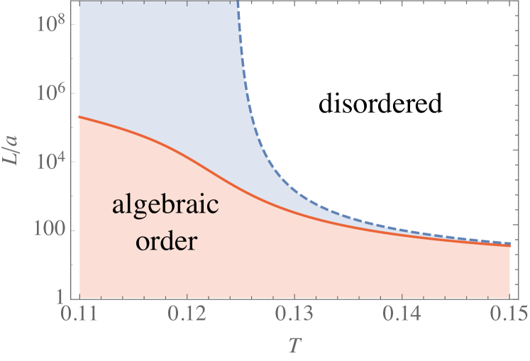
Figure 1: (Color online.) Finite-size phase diagram for a 2D driven-dissipative condensate. $T$ is the “vortex temperature,” i.e., the strength of the noise acting on topological defects, and $L$ is the system size measured here in units of a microscopic cutoff scale $a$. In thermal equilibrium (blue, dashed line), close to the critical temperature $T_{c}$, the phase boundary behaves as $\ln(L/a)\sim 1/\sqrt{T_{c}-T}$. Out of equilibrium (red, solid line), algebraic order is destroyed at any noise strength in the thermodynamic limit. For small values of $T$, the phase boundary approaches a value on the order of the bare screening length $L_{v}$. The phase boundaries are obtained by integrating the renormalization group flow equations (52) up to $y=1$, starting from an initial value of $y=0.1$.

Recently it has been noted Altman et al. (2015); Keeling et al. (2016); Gladilin et al. (2014); Ji et al. (2015); He et al. (2015) that the long wavelength fluctuations of a driven dissipative condensate map to a Kardar-Parisi-Zhang equation Kardar et al. (1986)

$$\partial_{t}\theta=D\nabla^{2}\theta+\frac{\lambda}{2}\left(\nabla\theta\right)^{2}+\eta,$$ (1)

where the condensate phase field $\theta(\mathbf{x},t)$ here plays the role of the height field $h(\mathbf{x},t)$ of the original interface growth problem, and the non-linearity $\lambda$ is proportional to the deviation from effective thermal equilibrium Altman et al. (2015). The renormalization group (RG) analysis of the KPZ equation shows that the non-linear term is relevant in two dimensions, exhibiting a flow to a strong coupling fixed point Canet et al. (2010, 2011); Canet (2012); Kloss et al. (2012) in which the interface is “rough,” or more precisely, height correlations increase as a power-law of distance ${\langle\left(h(\mathbf{x},t)-h(0,t)\right)^{2}\rangle}\sim\left\lvert\mathbf{x}\right\rvert^{2\chi}$, where $\chi>0$ denotes the “roughness exponent.” For the driven condensate problem the rough phase, corresponding to strongly non-linear fluctuations of the phase, is manifested by a stretched exponential decay of the condensate correlations. However, these correlations establish only beyond a large emergent length scale $L_{*}$, while at shorter distances the correlations can show algebraic decay as in equilibrium. Thus, the algebraic order observed in exciton-polaritons can only be a finite-size crossover phenomenon. This raises the question, whether the same is true for superfluidity: can a driven-dissipative condensate support a superfluid phase in the thermodynamic limit or will it ultimately be destroyed by diverging fluctuations?

There is a crucial difference between Eq. (1) and the KPZ equation that is not taken into account by the above considerations and is pertinent to the question of superfluidity. Contrary to the height field, the phase $\theta$ is compact, defined periodically on the interval $[0,2\pi)$, hence the phase admits topological defects that the conventional non-compact height field does not. This difference also arises in “active smectics” Chen and Toner (2013) and driven vortex lattices in disordered superconductors Aranson et al. (1998a). Similarly, the dynamics of the phase of sliding density waves Balents and Fisher (1995); Chen et al. (1996) and arrays of coupled limit-cycle oscillators Lauter et al. (2015, 2016) feature KPZ-type non-linearities. It may be natural to expect that the rapid (i.e., faster than power-law) decay of condensate correlations would lead to unbinding and proliferation of vortices rendering the strong coupling fixed point unstable. However this expectation is based on our understanding of the unbinding of vortices in the Kosterlitz-Thouless transition Kosterlitz and Thouless (1973); Berezinskii (1971, 1972), which is valid only in thermal equilibrium. On the other hand, we show below by direct analysis of the strong coupling KPZ fixed point (i.e., neglecting vortices), that such a state sustains a finite superfluid stiffness that may conceivably protect from proliferation of unbound vortices even if they were allowed. These seemingly conflicting considerations concerning the stability of a superfluid steady state highlight the need to account for the vortices within a comprehensive theory of the non-equilibrium condensate fluctuations.

In this paper, we incorporate vortices into the framework by establishing a duality between the compact KPZ equation (1) and a non-linear electrodynamics theory. Our heuristic derivation here is complemented by a more systematic approach with the same result in Sieberer et al. (2016b). The question of superfluidity is thereby translated into the problem of screening of charges (vortices) by the non-linear medium. As in equilibrium, if unbound charges proliferate, then they screen the electric field (circulating persistent current) emanating from a test charge, thus destroying the superfluid properties of the system.

We solve the non-linear screening problem within a perturbative renormalization group scheme valid for low vortex density and at length scales below the KPZ scale $L_{*}$, where the non-linearity $\lambda$ can be considered small. In the equilibrium case in which $\lambda=0$, and if the number of particles is conserved, our approach reproduces the standard linear electrodynamics of vortices in superfluid films Ambegaokar et al. (1978, 1980); Côté and Griffin (1986); Minnhagen (1987) exhibiting a Kosterlitz-Thouless transition, while out of equilibrium it allows us to systematically account for the effect of the non-linearity on the dynamics of vortices. The main effect of the non-linearity is to modify the force law between pairs of vortices so that they always unbind at length scales larger than the emergent scale $L_{v}$. The latter is exponentially large in the parameter $\lambda/D$, which we assume to be small for simplicity. Note that this length scale is different from the KPZ scale $L_{*}$, which is exponentially large in $g^{2}=\lambda^{2}\Delta/D^{3}$. In particular, the KPZ scale $L_{*}$ depends on the noise strength, whereas $L_{v}$ does not.

Indeed we note that the instability towards vortex unbinding has already been discussed in Ref. Aranson et al. (1998b) in the context of the complex Ginzburg-Landau equation and in Ref. Aranson et al. (1998a) for the driven vortex lattice. This result was based on solving the equations of motion of the vortices within the deterministic (i.e., noiseless) non-linear equations and in this way obtaining their mutual interaction. In this paper we come to this conclusion from a different angle, through derivation of the dual electrodynamic theory. This allows us not only to identify the instability, but also to predict and characterize the different crossover regimes using a renormalization group analysis. In particular, we characterize the crossover from Kosterlitz-Thouless equilibrium-like physics at intermediate scales to the unbinding governed by the non-equilibrium physics occurring at longer scales. Using the RG analysis we can estimate the regimes of parameters where the former physics would be observed in experiment and where the new emergent effects of the non-equilibrium fluctuations become dominant. This crossover is seen in the finite size phase diagram shown in Fig. 1.

II Superfluidity in a vortex-free driven-dissipative system

Before discussing the effect of vortices it is interesting to investigate the fate of superfluidity in a driven-dissipative system without topological defects. That is, we ask whether a system described by the KPZ equation (1) with a non-compact phase field has a superfluid response to an external vector potential. It is well known that within the standard analysis of the KT transition in the equilibrium $XY$ model the superfluid stiffness is not renormalized in absence of vortices. However, the KPZ equation provides an independent source of non-linearity that can potentially destroy superfluidity even without vortices. This possibility is perhaps further suggested by the fact that the non-linearity does lead to destruction of the condensate correlations, leading to (stretched) exponential rather than power-law decay.

Below we show that this naive expectation is in fact incorrect. In the absence of topological defects in the phase field, the physics of a 2D driven-dissipative condensate is governed by the strong-coupling fixed point of the non-compact KPZ equation. We show that this implies very peculiar properties: while correlations of the condensate field are short ranged, the response is superfluid. We stress again that this is the outcome only if we neglect the generation and possible proliferation of vortices.

In Ref. Keeling (2011), the superfluid density of a 2D driven-dissipative condensate was calculated using an expansion in fluctuations around the mean-field stationary state. Such an approach is valid when phase fluctuations remain small, i.e., when the nonlinear term in the KPZ equation is not dominant as in finite systems below the KPZ scale $L_{*}$. Also in this case the response is superfluid, however, the mechanism leading to this result is completely different from the one that yields the finite superfluid density we obtain below. We defer a detailed discussion of this point to Appendix B.

In the following, we work with the effective action that generates the KPZ equation (1),

$$S_{\mathrm{KPZ}}=\int d^{2}\mathbf{r}dt\,\hat{\theta}\left[\partial_{t}\theta-D\nabla^{2}\theta-\frac{\lambda}{2}\left(\nabla\theta\right)^{2}-\Delta\hat{\theta}\right].$$ (2)

The fields $\theta$ and $\hat{\theta}$ are independent variables. In the Martin-Siggia-Rose (MSR) framework Kamenev (2011); Altland and Simons (2010); Täuber (2014), $\hat{\theta}$ is termed the response field.

In presence of $U(1)$ symmetry, superfluidity can be defined in the driven open system — even without particle number conservation — through the response of the flow to gauging the $U(1)$ symmetry with an external vector potential. Formally, this is done through the usual replacement $\nabla\theta\to\nabla\theta-\mathbf{a}$; physically, the vector potential $\mathbf{a}$ can be introduced, e.g., in exciton-polaritons using the method described in Ref. Keeling (2011). Expanding the action to linear order in the applied vector potential we get $S[{\mathbf{a}}]=S_{\mathrm{KPZ}}-\int d^{2}{\bf r}dt\,{\mathbf{a}}\cdot\hat{\mathbf{j}}$. The object linearly coupled to the gauge field,

$$\hat{\mathbf{j}}=D\nabla\hat{\theta}-\lambda\hat{\theta}\nabla\theta,$$ (3)

is the Noether current associated with the $U(1)$ symmetry. It is not the physical particle current because the symmetry is not conjugate to particle number conservation Sieberer et al. (2016a). In absence of particle number conservation it is more subtle to identify the physical current ${\mathbf{j}}$ that responds to the applied force. This can be done by noting that in the extended system including also the bath degrees of freedom the number of particles is conserved. Hence one can define the total current density in this enlarged system and decompose it into two components: (i) the dissipative current flowing from the system into the bath, and (ii) the non-dissipative current which flows only in the system Avron et al. (2012); Gebauer and Car (2004). In our case, the non-dissipative current is given by the standard expression ${\mathbf{j}}=D\nabla\theta$ (see Keeling et al. (2014) for a proposal of an experimental procedure to address this current in microcavity polaritons by means of artificial gauge fields). Now the superfluid stiffness can be defined in terms of the linear response of this current to the applied vector potential:

$$\chi_{ij}(\mathbf{x}-\mathbf{x}^{\prime},t-t^{\prime})=\left.\frac{\delta\left\langle j_{i}(\mathbf{x},t)\right\rangle}{\delta a_{j}(\mathbf{x}^{\prime},t^{\prime})}\right\rvert_{\mathbf{a}=0}={\langle j_{i}(\mathbf{x},t)\hat{j}_{j}(\mathbf{x^{\prime}},t^{\prime})\rangle}.$$ (4)

The response function can be decomposed into two contributions, $\chi=\chi^{(1)}+\chi^{(2)}$, which are

$$\chi_{ij}^{(1)}(\mathbf{x}-\mathbf{x}^{\prime},t-t^{\prime}) =D^{2}\langle\partial_{i}\theta(\mathbf{x},t)\partial_{j}\hat{\theta}(\mathbf{x}^{\prime},t^{\prime})\rangle,$$ (5)

$$\chi_{ij}^{(2)}(\mathbf{x}-\mathbf{x}^{\prime},t-t^{\prime}) =D\lambda\langle\partial_{i}\theta(\mathbf{x},t)\partial_{j}\theta(\mathbf{x}^{\prime},t^{\prime})\hat{\theta}(\mathbf{x}^{\prime},t^{\prime})\rangle.$$ (6)

The superfluid stiffness in an isotropic system is directly related to the difference between the longitudinal and transverse parts of the Fourier transform of the response function at zero frequency in the long-wavelength limit Griffin (1994); Hohenberg and Martin (1965); Pitaevskii and Stringari (2003). (An alternative definition of the superfluid stiffness in terms of the oscillation frequency of the condensate was used in Refs. Janot et al. (2013); Gladilin and Wouters (2016). We note that these works did not consider the effect of fluctuations on the superfluid density.)

The contribution $\chi^{(1)}$ to the response function looks like the standard current-current response in equilibrium superfluids. Indeed, while $\chi^{(1)}$ is scale invariant at the Gaussian fixed point corresponding to an equilibrium superfluid, the contribution $\chi^{(2)}$ vanishes because it is the average of an odd number of fields. However, in the driven-dissipative case, the appropriate steady state (still ignoring vortices) is governed by the strong coupling fixed point of the KPZ equation. As we show in Appendix B, at this fixed point the contribution $\chi^{(1)}$ has a negative scaling dimension of $-\chi$, with $\chi$ being the roughness exponent of the strong coupling fixed point. Numerical simulations Kim and Kosterlitz (1989); Miranda and Aarão Reis (2008); Marinari et al. (2000); Ghaisas (2006); Chin and den Nijs (1999); Tang et al. (1992); Ala-Nissila et al. (1993); Castellano et al. (1999); Aarão Reis (2004); Kelling and Ódor (2011); Halpin-Healy (2012); Halpin-Healy and Lin (2014); Pagnani and Parisi (2015) and functional RG Canet et al. (2010, 2011); Canet (2012); Kloss et al. (2012) results find $\chi\approx 0.4$. Hence the conventional part of the current-current response function gives a vanishing contribution to the superfluid stiffness. On the other hand, $\chi^{(2)}$ is scale invariant at the strong coupling fixed point and leads to a constant superfluid stiffness.

We conclude that in a driven-dissipative condensate governed by KPZ dynamics the superfluid response is a non vanishing constant in spite of not having any long range or even algebraic order. However, as we mentioned before, this result assumes that the phase field behaves as a non-compact variable neglecting the existence and possible proliferation of topological defects in it. Below we develop a theory that incorporates the vortices into the general non-equilibrium framework.

III Dual electrodynamic theory

The force between point vortices in conventional two-dimensional superfluids falls off as the inverse distance, exactly as the force between two dimensional Coulomb charges. Such a duality mapping between vortices and electrostatics was famously exploited in the theory of the Kosterlitz-Thouless transition Kosterlitz and Thouless (1973); José et al. (1977, 1978); Savit (1980). The transition from the low-temperature superfluid to the high-temperature normal state is dual to a two-dimensional Coulomb gas undergoing a transition from bound dipoles to a plasma of free charges. The superfluid stiffness is, in the dual picture, given by the inverse dielectric constant of the Coulomb gas, which in the plasma phase falls to zero at long distances, due to effective screening of the Coulomb forces.

To investigate the stability of a superfluid in non-equilibrium conditions, we extend the duality to an electrodynamic theory that takes into account the dynamics under the influence of particle loss and external drive. In this paper we provide a simple heuristic derivation working with a continuum theory throughout. A systematic derivation of the same dual theory on a lattice is given in a parallel paper Sieberer et al. (2016b). We note in passing that in the context of zero-temperature superfluid-insulator transitions the vortex-charge duality has been extended to a complete quantum-electrodynamics theory Fisher and Lee (1989). In the system we consider, the non-equilibrium conditions of the condensate lead to a dual description in terms of classical electrodynamics with crucial modifications.

III.1 Modified Maxwell equations with charges

The starting point of the duality mapping is the usual low-frequency description of driven open Bose liquids, such as exciton-polariton systems, the stochastic Gross-Pitaevski or complex Landau-Ginzburg equation (CGLE) for the complex scalar order parameter Carusotto and Ciuti (2013),

$$\partial_{t}\psi({\bf r},t)=-{{\delta}H_{d}\over{\delta}\psi^{*}}-i{{\delta}H_{c}\over{\delta}\psi^{*}}+\zeta({\bf r},t).$$ (7)

$H_{\ell}$ ($\ell=c,d$) are effective Hamiltonians, which generate coherent and dissipative dynamics, respectively, and read for an isotropic situation

$$H_{\ell}=\int d^{2}{\bf r}\left[r_{\ell}|\psi|^{2}+K_{\ell}|\nabla\psi|^{2}+\frac{1}{2}u_{\ell}|\psi|^{4}\right]\leavevmode\nobreak\ .$$ (8)

The term $\zeta({\bf r},t)$ in Eq. (7) describes a Gaussian white noise with short-ranged spatio-temporal correlations ${\langle\zeta^{*}({\bf r},t)\zeta({\bf r}^{\prime},t^{\prime})\rangle}=2\sigma{\delta}({\bf r}-{\bf r}^{\prime}){\delta}(t-t^{\prime})\leavevmode\nobreak\ ,{\langle\zeta({\bf r},t)\zeta({\bf r}^{\prime},t^{\prime})\rangle}=0$, and zero mean. In the following, we set $K_{d}=0$ for simplicity, which also is a good approximation in exciton-polariton systems Carusotto and Ciuti (2013). It is straightforward to include this term and verify that it does not lead to a different effective theory.

The complex field $\psi(\mathbf{r},t)$ is conveniently split into two real variables in terms of the phase-amplitude representation,

$$\psi(\mathbf{r},t)=\sqrt{\bar{\rho}+\delta\!\rho(\mathbf{r},t)}e^{i\theta(\mathbf{r},t)}.$$ (9)

Here, the total density under the square root can be expanded in the fluctuations $\delta\!\rho(\mathbf{r},t)$ about the homogeneous background density $\bar{\rho}$, since density fluctuations are damped or gapped at long wavelength. In contrast, the phase fluctuations describe the Goldstone mode of the phase rotation symmetry at sufficiently low noise level, and thus are gapless (cf. e.g. the discussion in Altman et al. (2015)). Therefore, in the coupled stochastic equations of motion for phase and amplitude fluctuations, it is possible to directly integrate out the density mode, which leads to the KPZ equation (1)—an effective long-wavelength description for the phase mode, valid at scales well below the damping gap of the amplitude fluctuations Altman et al. (2015). The parameters appearing in the KPZ equation are related to those of the CGLE as $D=K_{c}u_{c}/u_{d}$ and $\lambda=-2K_{c}$, and the Gaussian noise field $\eta$ in Eq. (1) has white correlations with strength $\Delta=\sigma(u_{c}^{2}+u_{d}^{2})/(2u_{d}\bar{\rho})$,

$$\langle\eta({\bf r},t)\eta({\bf r}^{\prime},t^{\prime})\rangle=2\Delta\delta({\bf r}-{\bf r}^{\prime})\delta(t-t^{\prime}).$$ (10)

For exciton-polaritons, a more microscopic description can be formulated in terms of a generalized Gross-Pitaevskii equation for lower polaritons coupled to an excitonic reservoir Wouters and Carusotto (2007). The relations between the parameters entering this model and the KPZ parameters are summarized in Ref. Altman et al. (2015).

In the description of long-wavelength fluctuations of driven-dissipative condensates in terms of the KPZ equation (1), the compact nature of the phase variable is not manifest. To make it explicit and to introduce the main qualitative modification of the problem – the occurrence of vortices – in a direct way, we take here a different route based on a noisy electrodynamic theory dual to the description in terms of density and phase. More precisely, we first make the usual Ambegaokar et al. (1980); Fisher and Lee (1989) identifications of the boson density fluctuations with the magnetic field, and the phase gradient with the electric field:

$${\bf B}=B{\bf\hat{z}}=-\delta\!\rho\,\hat{\mathbf{z}},\quad{\bf E}=-{\bf\hat{z}}\times\nabla\theta.$$ (11)

The noisy hydrodynamic equations of the condensate can then be written as equations of electrodynamics in the medium. In particular, the noisy equation for the phase (density) fluctuations translates into a modified Ampère (Faraday) law. Most importantly, vortices are incorporated in this fomulation in a natural way as external charges and currents for the electromagnetic fields.

We begin with Ampère’s law resulting from the equation of motion of the phase. More generally speaking, it describes Euler’s equations for the momentum balance in the fluid,

$$\nabla\times{\bf B}-\frac{\varepsilon}{c}\frac{\partial{\bf E}}{\partial t}=\frac{2\pi}{c}{\bf J}_{m}.$$ (12)

The source term ${\bf J}_{m}$ includes both the vortex current density ${\bf J}_{v}$ (it turns out below that this term is not crucial, so we do not discuss it in detail here) and a source associated with the non-equilibrium drive that violates energy and momentum conservation:

$${\bf J}_{m}\equiv{\bf J}_{v}+\frac{1}{2\pi}{\bf\hat{z}}\times\nabla\left(\frac{\lambda}{2}E^{2}+\eta\right).$$ (13)

The speed of light takes the value $c=u_{c}$. We have introduced here a dielectric constant $\varepsilon$ for consistency, whose physical meaning is explained below Eq. (15).

Now we turn to Faraday’s law, associated to the density fluctuations. Indeed, in a conventional superfluid it stems from the continuity equation for the particle density. In a driven system with losses, however, we must add a source term to the continuity equation leading to a corresponding change to Faraday’s law as

$$\nabla\times{\bf E}+\frac{1}{c}\frac{\partial{\bf B}}{\partial t}+\gamma{\bf B}=0.$$ (14)

Here the dissipative coefficient $\gamma$ must appear from symmetry considerations. Below we relate it to the more microscopic parameters of the CGLE model (7). For completeness we note that the continuity equation derived from the CGLE of the driven condensate Altman et al. (2015) generically contains also a noise term. We omit it here since ultimately it will just add to the noise source already present in Eq. (12).

Two more equations are missing to complete the analogy to Maxwell’s equations. The homogenous Maxwell equation $\nabla\cdot{{\bf B}}=0$ is trivial in the two dimensional setting as ${\bf B}=B{\bf\hat{z}}$. The condition of irrotational flow (in the absence of vortices) translates to Gauss’ law for the electric field (as appropriate for the 2D case, the numerical factor on the RHS is $2\pi$ instead of the usual $4\pi$),

$$\nabla\cdot{\bf E}={2\pi\over\varepsilon}n_{v},$$ (15)

where the vortex density $n_{v}({\mathbf{r}})=\sum_{i}n_{i}\delta({\mathbf{r}}-{\mathbf{r}}_{i})$ acts as a source of the electric field. In constrast to the vortex current in Eq. (13), the vortex density will play a crucial role for the understaning ot the problem. Note the appearance of the dielectric constant $\varepsilon$ as in the analysis of the KT transition. It anticipates that upon coarse graining the electric field emanating from a test charge will be screened by fluctuations consisting of bound vortex pairs with separation smaller than the running cutoff scale. At the microscopic scale, where the above equations are formulated, it takes the value $\varepsilon=1$, but then will be substantially renormalized.

Finally, to have a complete dynamical description we must also supplement the equations for the fields (15), (12) and (14) with dynamics for the charges (vortices) subject to those fields. In principle the charges are affected both by the electric and magnetic forces. However, consistent with the assumption of over-damped dynamics we include only the electric forces Ambegaokar et al. (1980)

$$\frac{\partial{\bf r}_{i}}{\partial t}=\mu n_{i}{\bf E}({\bf r}_{i},t)+\bm{\xi}_{i},$$ (16)

where the vortex mobility $\mu$ is a free parameter of the theory, which in principle can be determined from numerical simulations of the CGLE equation. Note, however, that in reality the CGLE is not the full microscopic model of the system, but only an intermediate scale effective theory. Hence it is better to treat $\mu$ as a new independent variable. Assuming that the universal long-wavelength behavior does not depend on the value of $\mu$, below we consider the limit $\mu\ll D$. Then, the motion of vortices is slow as compared to the fluctuations of the fields, which greatly simplifies the theoretical analysis of the problem. $\bm{\xi}_{i}$ is a random force field on the vortices, which we take to be short range and time correlated

$$\langle\xi_{i\alpha}(t)\xi_{j\beta}(t^{\prime})\rangle=2\mu T\delta_{ij}\delta_{\alpha\beta}\delta(t-t^{\prime}).$$ (17)

Microscopically the effective temperature for the vortices and the phase noise $\eta$ should be closely related as they have the same origin. However upon rescaling they may flow independently and therefore we keep them as different quantities in the effective model. This is to be compared with the equilibrium case where one must have $T=\Delta/D$ at all scales. We further note that the dynamical equation (16) does not allow for creation and annihilation of vortices, however we will introduce an effective fugacity $y$ which tunes their density in the steady state.

We can easily make contact to the KPZ equation (1). Since we are interested in the low frequency limit, we can neglect $\dot{{\bf B}}$ compared to ${\bf B}$ in Eq. (14): at long scales the density fluctuations are over-damped. The magnetic field can thus be eliminated from the equations using the over-damped Faraday law ${\bf B}=-\gamma^{-1}\nabla\times{\bf E}$ . Plugging this as well as Gauss’ law (15) into (12) we obtain a dynamical equation for the electric field ${\bf E}$ alone,

$$\varepsilon\frac{\partial{\bf E}}{\partial t}=D\nabla^{2}{\bf E}-{\bf\hat{z}}\times\nabla\left(\frac{\lambda}{2}E^{2}+\eta\right)-{2\pi\over\varepsilon}D\nabla n_{v}-2\pi{\bf J}_{v}.$$ (18)

where $D\equiv c/\gamma$. Now it is easily verified that by setting the vortex current and density to zero and re-expressing the field in terms of $\nabla{\theta}$, we recover Eq. (1).

III.2 Maxwell action with charges

In this section we develop a functional integral formulation of the generating functional for dynamic observables. We then use this formulation to derive the effective interactions between the charges mediated by the fluctuating electromagnetic fields and study whether vortex anti-vortex pairs tend to unbind.

As in usual electrodynamics it is convenient to write the electric and magnetic fields in terms of gauge potentials which automatically solve the homogenous Maxwell equations. The relation between the gauge potentials and the fields is, however, altered due to the over-damped dynamics. We set:

$${\bf B}=\frac{1}{\gamma}\nabla\times{\bf A},\qquad\qquad{\bf E}=-\nabla\phi-{\bf A},$$ (19)

which differs from the usual relation, where $\partial_{t}{\bf A}$ instead of ${\bf A}$ appears in the definition of the electric field. The dynamical equations are then invariant under the local gauge transformation

$${\bf A}\to{\bf A}+\nabla\chi,\qquad\qquad\phi\to\phi-\chi$$ (20)

(here, $\chi$ appears instead of the usual $\partial_{t}\chi$ in the last relation). Note that this local gauge freedom reflects the parameterization of the electric and magnetic fields, and is not directly related to the global $U(1)$ invariance of the original phase degree of freedom. For our purposes it is sufficient to choose the following gauge

$$\frac{\partial\phi}{\partial t}+\frac{D}{\varepsilon}\nabla\cdot{\bf A}=0,$$ (21)

corresponding to the usual Lorentz gauge in electrodynamics. The gauge fields then obey the following equations

$$\frac{\partial\phi}{\partial t}-\frac{D}{\varepsilon}\nabla^{2}\phi = \frac{2\pi D}{\varepsilon^{2}}n_{v},$$ (22)

$$\frac{\partial{\bf A}}{\partial t}-\frac{D}{\varepsilon}\nabla^{2}{\bf A} = \frac{2\pi}{\varepsilon}{\bf J}_{v}+{{\bf\hat{z}}\times\nabla\over\varepsilon}\left(\frac{\lambda}{2}E^{2}+\eta\right).$$ (23)

Using the standard MSR framework we write a functional integral which generates the stochastic equations for the gauge fields (22) and (23) and $N$ charges

$$Z(N)=\int{\Delta}\hat{\phi}{\Delta}\phi\,{\Delta}\hat{\bf A}{\Delta}{\bf A}\,{\Delta}\hat{{\bf p}}{\Delta}{\bf r}\,e^{-S}.$$ (24)

Here we have already integrated over the gaussian noise fields $\eta$ and $\bm{\xi}$. The hatted fields are the response fields conjugate to those appearing in the equations of motion, which are introduced along the MSR construction. The action is a sum of the following contributions $S=S_{0}+S_{\lambda}+S_{c}+S_{\mathrm{int}}$. The quadratic free field action is given by

$$S_{0}=-\frac{1}{2}\int_{\mathbf{r},t}\begin{array}[]{cc}(\hat{A}_{\mu},&A_{\mu})\\ \end{array}\left(\begin{array}[]{cc}2\Delta_{\mu\nu}&\delta_{\mu\nu}L^{+}\\ \delta_{\mu\nu}L^{-}&0\end{array}\right)\left(\begin{array}[]{c}\hat{A}_{\nu}\\ A_{\nu}\end{array}\right),$$ (25)

where $\int_{\mathbf{r},t}=\int d^{2}\mathbf{r}dt$, $(\hat{A}_{\mu},A_{\mu})=(\hat{\phi},\hat{\bf A},\phi,{\bf A})$,  $L^{\pm}=\pm\partial_{t}-(D/\varepsilon)\nabla^{2}$, and

$$\Delta_{\mu\nu}=\Delta\left(1-\delta_{\mu 0}\right)\left(1-\delta_{\nu 0}\right)\left(\nabla^{2}\delta_{\mu\nu}-\partial_{\mu}\partial_{\nu}\right).$$ (26)

The non-linear contribution from the $\lambda$ term in the KPZ equation is given by

$$S_{\lambda}=-{\lambda\over 2\varepsilon}\int_{\mathbf{r},t}{\bf\hat{z}}\cdot\left(\hat{\bf A}\times\nabla(E^{2})\right),$$ (27)

where $E^{2}\equiv(\nabla\phi+{\bf A})^{2}$. The combined electromagnetic action $S_{em}=S_{0}+S_{\lambda}$, without coupling to the charges, provides an equivalent description of the standard non-compact KPZ equation in two dimensions. This is evident by noting that ${\bf v}={\bf\hat{z}}\times{\bf E}$ is equivalent to the vector field in Burgers’ equation Kardar et al. (1986).

The action of the charges is

$$S_{c}=-\sum_{i=1}^{N}\int dt\left(\hat{{\bf p}}_{i}\cdot\partial_{t}{\bf r}_{i}+\mu T\hat{p}_{i}^{2}\right),$$ (28)

while the coupling of charges to the gauge fields is given by

$$S_{\mathrm{int}}=\int_{\mathbf{r},t}\left(\frac{2\pi}{\varepsilon}\,J_{\mu}\hat{A}_{\mu}-\mu\,\hat{P}_{\mu}A_{\mu}\right).$$ (29)

In the above expression for the coupling action we have made use of the following notations:

$$J_{\mu} \equiv\left({D\over\varepsilon}\,n_{v},{\bf J}_{v}\right),$$ (30)

$$\hat{P}_{\mu} \equiv(-\nabla\cdot\hat{{\bf P}},\hat{{\bf P}}),$$ (31)

where

$$n_{v}({\bf r},t) =\sum_{i}n_{i}\delta({\bf r}-{\bf r}_{i}(t)),$$ (32)

$${\bf J}_{v}({\bf r},t) =\sum_{i}n_{i}\partial_{t}{\bf r}_{i}\delta({\bf r}-{\bf r}_{i}(t)),$$ (33)

$$\hat{{\bf P}}({\bf r},t) =\sum_{i}n_{i}\hat{{\bf p}}_{i}\delta({\bf r}-{\bf r}_{i}(t)).$$ (34)

Having derived a complete action describing dissipative non-linear electrodynamics (equivalent to KPZ dynamics) coupled to charges (vortices) we can deduce the effective interactions between the charges in certain limiting cases.

III.3 Charge interactions for weak nonlinearity

In the limit of small $\lambda$ we can integrate over the photon fields perturbatively in the non-linear coupling with respect to the quadratic photon action $S_{0}$. For $\lambda=0$ the effective action for the charges can be obtained exactly by direct integration over the gauge fields

$$S_{I}^{(0)} = \frac{1}{2}\int_{{\bf r},t;{\bf r}^{\prime},t^{\prime}}\begin{pmatrix}2\pi J_{\mu}/\varepsilon,&-\mu\hat{P}_{\mu}\end{pmatrix}_{{\bf r},t}\times$$ (35)

$$\begin{pmatrix}0&\delta_{\mu\nu}g^{-}\\ \delta_{\mu\nu}g^{+}&-2g^{+}\Delta_{\mu\nu}g^{-}\end{pmatrix}_{{\bf r},t;{\bf r}^{\prime},t^{\prime}}\begin{pmatrix}2\pi J_{\nu}/\varepsilon\\ -\mu\hat{P}_{\nu}\end{pmatrix}_{{\bf r}^{\prime},t^{\prime}},$$

where $g^{\pm}=(L^{\pm})^{-1}$.

Noting that vortices move very slowly in the $\mu/D\to 0$ limit, we find that the most relevant contribution comes from the static $J_{0}P_{0}$ term, which is linear in $\mu$, while all other terms are of higher order. Let us denote the static free Green’s function as

$$G(\mathbf{r}-\mathbf{r}^{\prime})=-\nabla^{-2}\delta(\mathbf{r}-\mathbf{r}^{\prime})\simeq-\frac{1}{2\pi}\ln(|{\bf r}-{\bf r}^{\prime}|/a).$$ (36)

This gives

$$\begin{split}S_{I}^{(0)}&\simeq-\int_{t}\sum_{ij}\hat{\bf p}_{i}(t)\cdot\mu n_{i}\nabla_{i}G({\bf r}_{i}-{\bf r}_{j})\frac{2\pi n_{j}}{\varepsilon},\end{split}$$ (37)

which, as expected, describes the 2D Coulomb gas interactions. To see this we note that the action for a Brownian particle contains the term $\int dt\,\mu\hat{\bf p}\cdot{\bf f}_{0}$, where $\bf f_{0}$ is the force acting on the particle. For further reference we note here that, when this happens to be a conserving force, ${\bf f}_{0}=-\nabla V$, the stationary solution of the corresponding Fokker-Planck equation is just the Gibbs distribution, $P({\bf r})\sim e^{-V({\bf r})/T}$.

Our goal is to calculate the effective mutual forces between two opposite charges, perturbatively in $\lambda$, in order to determine the fate of the Kosterlitz-Thouless transition in the presence of the non-linear term. This task is greatly simplified in the limit $\mu/D\to 0$, since the fields’ response is instantaneous on the time scales of the vortices’ motion. Thus, there are two stages in the calculation of the forces to a given order $O(\lambda^{m})$: (i) calculation of the $O(\lambda^{m})$ terms in the effective charge action, $S_{I}^{(m)}$. (ii) taking the limit $\mu/D\to 0$, and identifying the force as the coefficient of $\hat{\bf p}_{i}$ linear in $\mu$.

In what follows we consider the interaction between a vortex ($n_{+}=1$) at $\mathbf{r}_{+}$ and an antivortex ($n_{-}=-1$) at $\mathbf{r}_{-}$. We begin by determining the correction to the Coulomb law linear in $\lambda$. The correction to the action contains one term (corresponding to a tree level diagram)

$$S_{I}^{(1)}=\frac{2\pi^{2}\lambda\mu{\bf\hat{z}}}{\varepsilon^{3}}\cdot\int_{1234}\hat{\bf P}({\bf r}_{1},t_{1})g^{+}({\bf r}_{1}-{\bf r}_{2},t_{1}-t_{2})\times\bm{\nabla}_{2}\left(g^{+}({\bf r}_{2}-{\bf r}_{3},t_{2}-t_{3})J_{\mu}({\bf r}_{3},t_{3})g^{+}({\bf r}_{2}-{\bf r}_{4},t_{2}-t_{4})J_{\mu}({\bf r}_{4},t_{4})\right),$$ (38)

where $\int_{1\dots M}=\prod_{i=1}^{M}\int_{{\bf r}_{i},t_{i}}$. Note that this term is second order in $J_{\mu}$, demonstrating the breakdown of force superposition for $\lambda\neq 0$. In the limit $\mu/D\to 0$, only static $J_{\mu}({\bf r},t)=(J_{0}({\bf r}),0)$ configurations contribute to the MSR integral, giving

$$S_{I}^{(1)}\simeq-\frac{\varepsilon\lambda}{4\pi D}\int_{\mathbf{r},t}\mu\hat{\mathbf{p}}_{+}\cdot\left({\bf\hat{z}}\times{\bf f}_{0}(\mathbf{r}_{+}-\mathbf{r})\right)\left|{\bf f}_{0}({\bf r}-\mathbf{r}_{+})-\mathbf{f}_{0}(\mathbf{r}-\mathbf{r}_{-})\right|^{2}-(+\leftrightarrow-)\equiv\int_{t}\mu\hat{\mathbf{p}}_{+}\cdot\mathbf{f}^{(1)}(\mathbf{r}_{+}-\mathbf{r}_{-})-(+\leftrightarrow-).$$ (39)

For simplicity we have denoted, $\mathbf{f}_{0}(\mathbf{r})\equiv\left(2\pi/\varepsilon\right)\nabla G(\mathbf{r})=-\mathbf{r}/(\varepsilon r^{2})$. The $O(\lambda)$ correction to the force for $\left\lvert\mathbf{r}_{+}-\mathbf{r}_{-}\right\rvert/a\gg 1$ is given by (see Appendix A)

$$\mathbf{f}^{(1)}(\mathbf{R})=-\frac{\lambda}{2D\varepsilon^{2}}\frac{\hat{\mathbf{z}}\times\mathbf{R}}{R^{2}}\left(2\ln(R/a)-\frac{1}{2}\right).$$ (40)

This force acts on the dipole in a direction perpendicular to the segment $\mathbf{R}=\mathbf{r}_{+}-\mathbf{r}_{-}$. Hence, the first order correction does not affect the probability distribution of the vortex-dipole sizes.

We next calculate the $O(\lambda^{2})$ correction to the force. There are two types of corrections to the effective action, $S_{I}^{(2)}$, at this order. The first involves fluctuation correlations (corresponding to loop diagrams), and modifies the $J_{\mu}\hat{P}_{\nu}$ and $\hat{P}_{\mu}\hat{P}_{\nu}$ terms, which appear in the zeroth-order charge action, Eq. (35). These can be treated only within a Renormalization Group framework, due to infrared divergences. Nevertheless, they do not modify the effective force: the modified $J_{\mu}\hat{P}_{\nu}$ term vanishes in two dimensions Kardar et al. (1986), and the $\hat{P}_{\mu}\hat{P}_{\nu}$ term is of order $O(\mu^{2})$, which we neglect in the $\mu/D\to 0$ limit. The second type (corresponding to tree level diagrams) is third order in $J_{\mu}$, which, in the limit $\mu/D\to 0$ becomes

$$\begin{split}S_{I}^{(2)}&\sim-\frac{\lambda^{2}\varepsilon^{2}}{16\pi^{2}D^{2}}\sum_{i,j,k=\pm}\int_{{\bf r},{\bf r}^{\prime},t}\mu\hat{\mathbf{p}}_{+}\cdot\left({\bf\hat{z}}\times{\bf f}_{0}({\bf r}_{+}-{\bf r})\right)n_{i}{\bf f}_{0}({\bf r}-{\bf r}_{i})\cdot\left({\bf\hat{z}}\times{\bf f}_{0}({\bf r}-{\bf r}^{\prime})\right)n_{j}{\bf f}_{0}({\bf r}^{\prime}-{\bf r}_{j})\cdot n_{k}{\bf f}_{0}({\bf r}^{\prime}-{\bf r}_{k})-(+\leftrightarrow-)\\ &\equiv\int dt\,\mu\hat{\mathbf{p}}_{+}\cdot\mathbf{f}^{(2)}({\bf r}_{+}-{\bf r}_{-})+(+\leftrightarrow-).\end{split}$$ (41)

The correction to the force between two particles of opposite charge and distance $R\gg a$ is evaluated in Appendix A, with the result

$$\mathbf{f}^{(2)}(\mathbf{R})=\frac{1}{8}\left(\frac{\lambda}{2D}\right)^{2}\frac{1}{\varepsilon^{3}}\frac{\mathbf{R}}{R^{2}}\left(8\ln(R/a)^{2}+4\ln(R/a)-1\right).$$ (42)

Note that this is a central force that constitutes a repulsive contribution to the attractive $1/R$ Coulomb law. The last term merely renormalizes the bare value of the dielectric constant $\varepsilon$. We omit it in the following.

The effective interactions computed above (see Appendix A) hold as long as the perturbation theory in $\lambda$ is valid. From this result it is clear that the second order correction becomes larger than the zeroth order term beyond a separation of

$$L_{v}=a\,e^{\frac{2D}{\lambda}},$$ (43)

where we took the bare value of $\varepsilon$ to be $1$. Furthermore perturbation theory in $\lambda$ fails beyond the emergent KPZ length scale $L_{*}=a\exp(8\pi D^{3}/(\Delta\lambda^{2}))$. Before proceeding we comment on how the corrections to the force, found above, are related to the flow field around vortices. Consider first a single vortex solution to the stationary KPZ equation $D\nabla\cdot{\bf v}+(\lambda/2){\bf v}^{2}=0$, with ${\bf v}=\nabla{\theta}$. It is easily seen that the velocity field with a vortex in the azimuthal component $v_{\varphi}=1/r$ produces a radial component $v_{r}(r)\sim-(\lambda/2r)\ln r$ at large $r$. This structure of a vortex is well known in the literature on complex Ginzburg-Landau equations, where it is termed a Zhabotinsky spiral Aranson and Kramer (2002). The first order correction to the Coulomb force is a direct result of this radial flow - recall that the electric field is ${\bf E}=-{\bf\hat{z}}\times{\bf v}$. Hence the azimuthal flow $v_{\varphi}$ leads to the usual Coulomb force, while the radial flow leads to a force perpendicular to it.

The second order correction is due to the interaction between the flow fields of the two vortices. It cannot be explained based on the flow around a single vortex because the two flows (phases) do not superpose in this non-linear flow equation. Together with $\mathbf{f}_{0}$ and in contrast to $\mathbf{f}^{(1)}$, it contributes to the central part of the force between the vortex-antivortex pair, $\mathbf{f}_{c}({\bf r})=\mathbf{f}_{0}({\bf r})+\mathbf{f}^{(2)}({\bf r})$, where ${\bf r}$ is the relative coordinate between the vortices. This force is again conservative, and we have the effective potential $V_{\mathrm{eff}}=-\nabla\mathbf{f}_{c}$ including an external electric field,

$$V_{\mathrm{eff}}(\mathbf{r},\mathbf{E})\approx\frac{1}{\varepsilon}\ln(r/a)-\mathbf{E}\cdot\mathbf{r}\\ -\frac{\lambda^{2}}{12\varepsilon^{3}D^{2}}\left(\ln(r/a)^{3}+c\ln(r/a)^{2}\right),$$ (44)

where $D$ is the diffusion coefficient from the original KPZ equation. Anticipating independent renormalization of the terms in the potential, we include a coefficient $c$ with bare value $c_{0}=3/4$. Because there is an effective potential, the probability for finding the pair separated by $\bf r$ follows a Gibbs distribution:

$$P(\mathbf{r},\mathbf{E})=y^{2}e^{-V_{\mathrm{eff}}(\mathbf{r},\mathbf{E})/T}.$$ (45)

Here we defined $y^{2}$, the vortex fugacity, as the probability of having a pair with a separation of the value of the the short distance cutoff $a$. The existence of a vortex “temperature” $T$ is due to the conservative nature of the force between them. However, we emphasize again that due to the absence of global detailed balance, this temperature does not have to coincide with the noise level of the spin waves.

IV Vortex unbinding at small $\lambda$

Having obtained the effective interactions between vortices we are ready to address the central question of this paper concerning the superfluid properties of the driven condensate. A crucial observation pertinent to this issue is that the (inverse) static dielectric constant defined in Eq. (15) is a direct measure of the superfluid stiffness, $\rho_{s}$, as defined in Eq. (94). To see this, note that fixing a vortex at the origin is equivalent to gauging the flow with a transverse vector potential ${\bf a}={\bf\hat{z}}\times\hat{\bf r}/R$ (this is a vector potential that couples to the particle currents, not the dual vector potential coupled to the vortex currents). With no other vortices present the superfluid response, i.e., the transverse current induced by the vector potential, can be deduced directly from Gauss’ law. Noting the duality correspondence $\nabla\theta={\bf\hat{z}}\times{\bf E}$ and its relation to the particle current ${\bf j}=D\nabla\theta$, we have ${\bf j}=D{\bf\hat{z}}\times{\bf E}=D{\bf\hat{z}}\times\hat{\bf r}/{\varepsilon R}=(D/\varepsilon){\bf a}\equiv\rho_{s}{\bf a}$, where the electric field due to a vortex at the origin is ${\bf E}=\hat{\bf r}/\varepsilon R$. In the presence of noise, on the other hand, more pairs of charges can be generated and potentially screen the test charge placed at the origin. This screening, leading to a renormalized reduced value of $\varepsilon^{-1}$, is the dual description of the renormalized superfluid stiffness.

The question of superfluidity is thus mapped, as in the coventional Kosterlitz-Thouless transition, to the problem of screening in the Coulomb gas, albeit now with interactions modified by the KPZ nonlinearity. We consider the limit of zero vortex mobility $\mu/D\to 0$, where the vortex interactions are described by a static effective potential, derived in Sec. III.3 above in the limit of small $\lambda$. The dielectric constant is computed in this regime using a renormalization group scheme essentially identical to the one used to describe the KT transition José et al. (1977, 1978).

We begin by calculating the linear response of the ensemble averaged polarization density to an applied electric field, ${\langle\bf\Pi\rangle}=\chi\mathbf{E}$. It can be computed based on the effective Gibbs distribution for the vortex-antivortex potential Eq. (45); to linear order in the external field $\mathbf{E}$, it is given by

$$\begin{split}\langle\bf{\Pi}\rangle&=\frac{1}{L^{2}}\int\frac{d^{2}\mathbf{R}}{a^{2}}\frac{d^{2}\mathbf{r}}{a^{2}}\mathbf{r}P(\mathbf{r},0)\left(1+\frac{\mathbf{E}\cdot\mathbf{r}}{T}\right)\\ &=\frac{\pi y^{2}}{T}\int_{a}^{\infty}\frac{dr}{a}\left(\frac{r}{a}\right)^{3-\frac{1}{\varepsilon T}}e^{\frac{\lambda^{2}}{12\varepsilon^{3}D^{2}T}\left(\ln(r/a)^{3}+c\ln(r/a)^{2}\right)}\mathbf{E}\\ &=\chi\mathbf{E}.\end{split}$$ (46)

We have $1/L^{2}$ in front, since we are considering the contribution of one dipole to the polarization density. The two area integrals with measure $1/a^{2}$ act as the sum over all configuration of the single dipole, weighted by the probability, Eq. (45), and from which we read off the susceptibility:

$$\begin{split}\chi=\frac{\pi y^{2}}{T}\int_{a}^{\infty}\frac{dr}{a}\left(\frac{r}{a}\right)^{3-\frac{1}{\varepsilon T}}e^{\frac{\lambda^{2}}{12\varepsilon^{3}D^{2}T}\left(\ln(r/a)^{3}+c\ln(r/a)^{2}\right)}.\end{split}$$ (47)

The fully renormalized dielectric constant at the largest scales is given by $\varepsilon_{R}=\varepsilon+2\pi\chi$. As in the conventional Coulomb gas, this equation is solved using the renormalization group by gradually increasing the short distance cutoff at infinitesimal steps from $a$ to $a\left(1+d\ell\right)$. Separating the above integral into two parts

$$\int_{a}^{\infty}=\int_{a}^{a\left(1+d\ell\right)}+\int_{a\left(1+d\ell\right)}^{\infty},$$ (48)

allows to define the dielectric constant at the new cutoff

$$\varepsilon^{\prime}=\varepsilon+\frac{2\pi^{2}y^{2}}{T}d\ell.$$ (49)

A renormalization of the other couplings is required to bring the expression for $\varepsilon_{R}$ to its original form, Eq. (47),

$$\begin{split}\varepsilon_{R}&\approx\varepsilon^{\prime}+\frac{2\pi^{2}y^{2}}{T}\left[1+\left(4-\frac{1}{\varepsilon T}\right)d\ell\right]\int_{a}^{\infty}\frac{dr}{a}\left(\frac{r}{a}\right)^{3-\frac{1}{\varepsilon T}\left(1-\frac{c\lambda^{2}}{6\varepsilon^{2}D^{2}}d\ell\right)}e^{\frac{\lambda^{2}}{12\varepsilon^{3}D^{2}T}\left[\ln(r/a)^{3}+\left(c+3d\ell\right)\ln(r/a)^{2}\right]}\\ &=\varepsilon^{\prime}+\frac{2\pi^{2}y^{\prime 2}}{T^{\prime}}\int_{a}^{\infty}\frac{dr}{a}\left(\frac{r}{a}\right)^{3-\frac{1}{\varepsilon T^{\prime}}}e^{\frac{\lambda^{2}}{12\varepsilon^{3}D^{2}T}\left[\ln(r/a)^{3}+c^{\prime}\ln(r/a)^{2}\right]}.\end{split}$$ (50)

To obtain the last line we have the following rescaling constraints

$$\begin{split}\frac{y^{\prime 2}}{T^{\prime}}&=\frac{y^{2}}{T}\left[1+\left(4-\frac{1}{\varepsilon T}\right)d\ell\right],\\ \frac{1}{T^{\prime}}&=\frac{1}{T}\left(1-\frac{c\lambda^{2}}{6\varepsilon^{2}D^{2}}d\ell\right),\\ c^{\prime}&=c+3d\ell.\end{split}$$ (51)

In these RG equations we neglect corrections of order $y^{2}$ and $\lambda^{4}$ to the effective dipole energy. The differential RG equation for $c$ can be solved immediately and yields $c=c_{0}+3\ell$ with the bare value $c_{0}=3/4$. Inserting this result in the flow equations for the remaining couplings, we obtain

$$\begin{split}\frac{d\varepsilon}{d\ell}&=\frac{2\pi^{2}y^{2}}{T},\\ \frac{dy}{d\ell}&=\left[2-\frac{1}{2\varepsilon T}+\frac{\lambda^{2}}{4\varepsilon^{2}D^{2}}\left(\frac{1}{4}+\ell\right)\right]y,\\ \frac{dT}{d\ell}&=\frac{\lambda^{2}T}{2\varepsilon^{2}D^{2}}\left(\frac{1}{4}+\ell\right).\end{split}$$ (52)

Not surprisingly these flow equations are very similar to the KT scaling equations and collapse to the latter for $\lambda=0$. The effect of the non-linearity is to always drive the system to the high temperature (plasma) phase in which charges are perfectly screened. However this screening is achieved only at large length scales, bounded from below by the bare vortex unbinding length $L_{v}=a\exp(2D/\lambda)$.

The RG flow projected onto the two parameter space of $y$ versus $\varepsilon T$ is shown in Fig. 2. At a finite value of $\lambda$, the flow is seen to initially closely follow the KT flow at $\lambda=0$, approaching the fixed line at $y=0$, but ultimately departing from it in a flow toward the high temperature plasma phase.

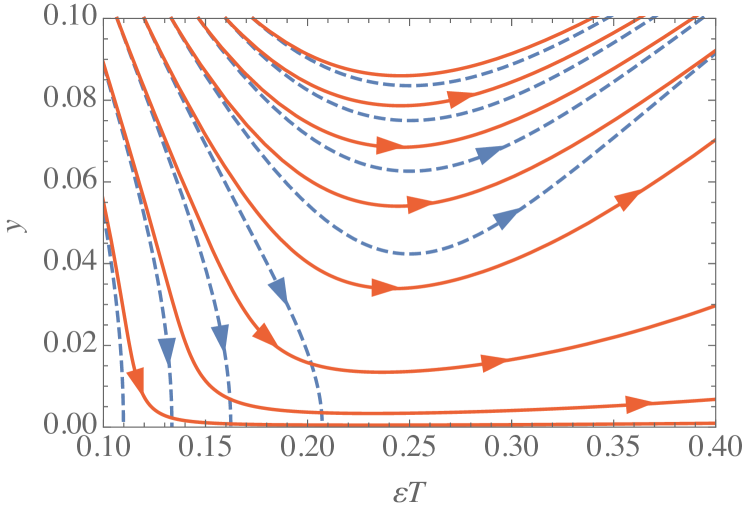
Figure 2: (Color online.) RG flow lines as described by Eqs. (52). Dashed: $\lambda=0$, KT flow; Solid: $\lambda^{2}/D^{2}=0.4$.

Figure 3 shows the dependence of $\varepsilon^{-1}$ (equal to the superfluid stiffness) on the (bare) effective vortex temperature $T$ computed from the RG flow for different system sizes. In practice, the bare effective temperature is related to the noise appearing in the KPZ equation. It is varied by tuning the pump power as described in Ref. Altman et al. (2015), where increasing pump power reduces this bare temperature. In an infinite system at thermal equilibrium (i.e., $\lambda=0$) the quantity $1/(\varepsilon T)$ undergoes a universal jump from zero to $1/(\varepsilon T)=4$ upon crossing the $KT$ transition temperature. This sharp feature is of course smeared in finite size systems, which are seen to very slowly approach this step as their size is increased (Fig. 3 (a)). In the driven system ($\lambda\neq 0$), $\epsilon^{-1}$ always vanishes in the thermodynamic limit regardless of the bare temperature. However, the finite size scaling behavior is non-trivial. If $\lambda$ is not too small the distinction from the $KT$ scaling behavior is already apparent at reasonable system sizes: rather than converging to a universal step at a critical $T$, the step is seen to be receding toward zero temperature.

Note that in Fig. 3 we are plotting the product of the renormalized dielectric constant $\varepsilon$ with the microscopic or bare value of the effective vortex temperature $T$. In experiments the microscopic value of $T$ will be known as it is directly controlled by tuning the pump power as explained above. On the other hand, the inverse dielectric constant corresponds to the superfluid stiffness. A macroscopic measurement of the stiffness can be implemented, as discussed above, by imposing a vortex at the origin and measuring the decay of the physical current at a long distance $R$ from it. This will give the fully renormalized value of $\varepsilon^{-1}$.

In exciton-polariton condensates, vortices can be imprinted both under conditions of coherent Sanvitto et al. (2010); Boulier et al. (2016) and incoherent pumping Dall et al. (2014). For a scheme to measure the current see Ref. Keeling et al. (2016). From the current, the response function (4) and hence the superfluid density can be reconstructed.

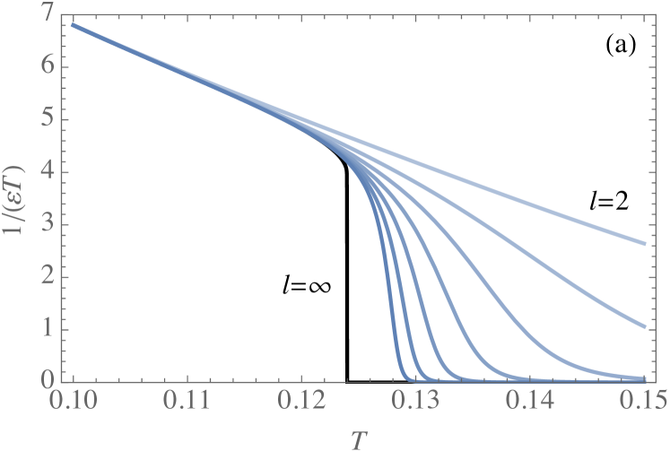
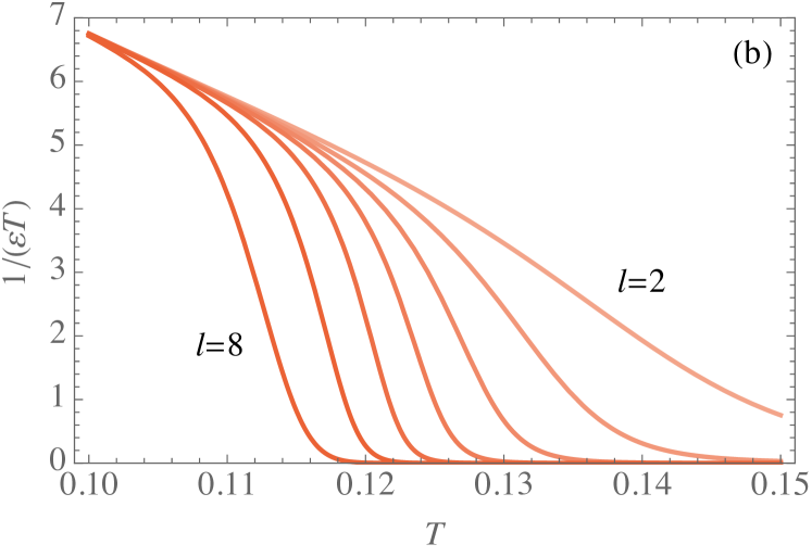
Figure 3: (Color online.) Renormalized dilectric constant in a finite-size system, obtained by integrating the RG flow equations (52). (a) 2D superfluid in thermal equilibrium, i.e., with $\lambda=0$. From top to bottom, the lines correspond to increasing system sizes. $l=2,3,\dotsc,8,\infty$ denotes the logarithmic system size $l=\ln(L/a)$. In the thermodynamic limit, the dielectric constant undergoes a discontinuous jump at the critical temperature from zero to the universal value $1/(\varepsilon T)=4$. (b) Non-equilibrium RG flow with $\lambda^{2}/D^{2}=0.15$. The qualitative behavior of $1/(\varepsilon T)$ closely resembles the equilibrium one of panel (a) up to moderate system sizes. For small values of $\lambda/D$, the agreement is even quantitative, and in finite-size systems equilibrium and driven-dissipative cases are practically indistinguishable. The non-equilibrium character of the underlying dynamics becomes manifest only in the thermodynamic limit, when $1/(\varepsilon T)$ is renormalized to zero. In both panels, $T$ is the bare value of the temperature, while $\varepsilon$ is the renormalized dielectric constant.

Another signature of the unbinding of vortices is the suppression of algebraic order on scales beyond the phase boundary of the finite-size phase diagram in Fig. 1. On larger scales, we expect correlations to decay rapidly due to the dephasing that is caused by vortices. In thermal equilibrium, the decay of correlations in the high-temperature phase above the KT transition can be shown to be exponential by means of a high-temperature expansion Chaikin and Lubensky (1995) which, however, cannot be generalized straightforwardly to the strong noise limit under non-equilibrium conditions. Still it is reasonable to assume that the form of the decay of correlations due to vortices is still exponential for finite values of $\lambda$. The main challenge for observing the suppression of algebraic order experimentally with exciton-polaritons is due to the large length scale at which it is expected to occur — note, however, that generically the phase boundary in the finite size phase diagram Fig. 1 is well below $L_{*}$, making the observation of the destruction of order more promising than originally anticipated based on a treatment that neglected vortices Altman et al. (2015). The precise location of the phase boundary is controlled by the parameter lambda. As discussed in Altman et al. (2015), in incoherently pumped systems this parameter is typically small, which was also assumed in our treatment. Quite intuitively, for this parameter to become sizable, one should use a cavity of lower quality, thus making polaritons short-lived and hindering thermalization. We can obtain a rough estimate of the location of the phase boundary based on the relations between the parameters in a more microscopic model of lower polaritons coupled to a high-energy near excitonic reservoir Wouters and Carusotto (2007) and the parameters of the KPZ equation derived in Ref. Altman et al. (2015). These relations lead to the following expressions for the (absolute value of) $\lambda/D$ and the vortex temperature $T$:

$$\frac{\lambda}{D} =\frac{2\bar{\gamma}}{1+x},$$ (53)

$$T =\frac{\Delta}{D}=\frac{\bar{u}\bar{\gamma}^{2}}{2x\left(1+x\right)}\left[1+\frac{\left(1+x\right)^{2}}{\bar{\gamma}^{2}}\right].$$ (54)

Here, $x$ is the dimensionless pumping strength, and $\bar{\gamma}$ and $\bar{u}$ are dimensionless parameters which, for the experimental parameters reported in Lagoudakis et al. (2008), take the values $\bar{\gamma}\approx 0.1$ and $\bar{u}\approx 0.14$ Altman et al. (2015). The mean-field condensation threshold is at $x=0$ where $T$ diverges. Note that also the KPZ non-linearity $\lambda$ depends on the pumping strength.

Figure 4 shows the finite-size phase diagram for incoherently pumped exciton-polaritons. The phase boundaries between algebraically ordered (shaded regions) and disordered phases are plotted against the pumping strength $x$ in panel (a) and the fugacity in panel (b). In both panels, the red, solid line corresponds to the values of $\bar{\gamma}$ and $\bar{u}$ given above. For comparison, the blue dashed line is obtained from the equilibrium KT flow. The small values of $\lambda/D$ (for $x$ in the range from $0.8$ to $1.8$ as shown in the figure $\lambda/D$ takes values from $0.07$ to $0.11$) lead to a phase boundary that follows very closely the equilibrium result. Above the equilibrium critical pump strength $x_{\mathrm{KT}}\approx 1.30$, the phase boundary is beyond any reasonable system size (note the logarithmic scale). A significant decrease of the phase boundary can be achieved by increasing the value of $\lambda/D$ which, according to Eq. (53), necessitates a higher value of $\bar{\gamma}$. Already an increase of $\bar{\gamma}$ by a factor of $5$ (corresponding to an increase of the cavity loss rate by the same factor) leads to a substantial decrease of the phase boundary (see the green, dotted-dashed line in Fig. 4).

The estimates of the phase boundary presented in Fig. 4 (a) are obtained by integrating the RG flow equations (52) from the ad hoc chosen microscopic value $y=0.1$ up to $y=1$. The dependence of these estimates on the microscopic value of the fugacity is shown in panel (b) of the same figure. Here, $x$ is set to the critical value of panel (a). Note that when $y$ is below its critical value in equilibrium, the phase boundary for the increased valued of $\bar{\gamma}$ (green, dotted-dashed line) stays on a plateau for a wide range of values of $y$, indicating that at least in this parameter regime our estimate of the phase boundary is not very sensitive to the unknown microscopic value of $y$. In order to determine $y$ experimentally it would be necessary to be able to obtain the distribution of vortices in single-shot experiments, which is at present not possible with exciton-polaritons.

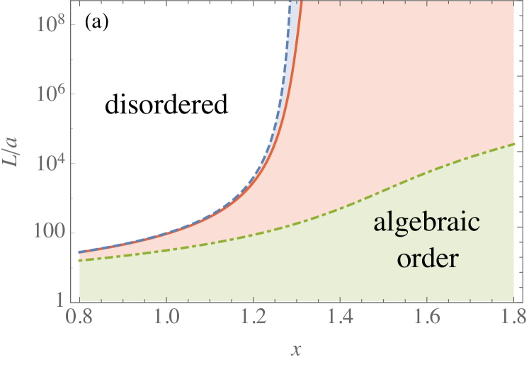
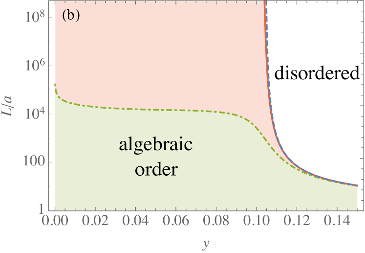
Figure 4: (Color online.) Finite size phase diagram as a function of (a) the dimentionless pumping strength, $x$, and (b) the vortex fugacity $y$. In both panels, the red, solid line denotes the boundary between disordered and algebraic order phases for $\bar{\gamma}=0.1$ and $\bar{u}=0.14$, the green, dotted-dashed line denote the same boundary with $\bar{\gamma}=0.5$, and the blue, dashed line is the KT phase boundary. In exciton-polaritons, the microscopic scale $a$ can be estimated as the healing length, which is typically $a\approx 1\,\mu\mathrm{m}$, while typical system sizes are on the order of $L\approx 100\,\mu\mathrm{m}$.

V Observability of KPZ scaling

We have seen that vortices are always relevant, and ultimately unbind in a driven condensate. Moreover, this occurs on a length scale $L_{v}$ that is generally much smaller than the scale $L_{*}$ on which the strong coupling KPZ physics would emerge in absence of topological defects. Hence, one might be tempted to conclude that the physics of the strong coupling KPZ fixed point is preempted by vortex proliferation and therefore irrelevant for two-dimensional driven condensates. However, our discussion so far has addressed only static properties, such as superfluid stiffness and spatial correlations strictly at steady state. In order to assess if KPZ scaling can be seen in experiments (or numerics based on evolving stochastic equations for the polariton amplitude, cf. e.g. Dagvadorj et al. (2015)) measuring time-dependent quantities, we must consider the dynamics of vortex unbinding.

As an example of a dynamical measurement we consider a quench experiment similar to that discussed in Ref. He et al. (2015). The system is first pumped coherently to prepare a condensate with an imprinted phase pattern. Hence the system is initialized as an almost perfect condensate with no free topological defects besides those that are imprinted externally. A useful initial configuration, at least for a Gedankenexperiment, has a vortex in a hole in the middle of the sample. From time $t=0$ onward the coherent pumping (i.e., phase imprinting) stops, leaving only the incoherent drive. The experiment then monitors the development of the spatial correlations as a function of time.

We need to consider two important time scales: (i) the time $\tau_{v}$ it takes for vortices to unbind and proliferate (or to nucleate at the boundary), leading to a decay of the superfluid current, should be compared with (ii) the time scale $\tau_{*}$ for development of the KPZ correlations. The characteristic time on which strong coupling KPZ scaling emerges in a system with no topological defects is related to the length scale $L_{*}$ by simple diffusive scaling

$$\tau_{*}=D^{-1}L_{*}^{2}\approx a^{2}D^{-1}e^{16\pi D^{3}\over\Delta\lambda^{2}}\equiv a^{2}D^{-1}e^{16\pi/g^{2}},$$ (55)

where $a$ is the microscopic length scale and $g^{2}\equiv\lambda^{2}\Delta/D^{3}$ is the dimensionless bare coupling constant of the KPZ equation Kardar et al. (1986). When the time evolution begins, vortices are absent or tightly bound in pairs on a microscopic scale. The time scale $\tau_{v}$ on which vortices unbind can be estimated based on the stochastic equation (16) for the relative coordinate of a vortex pair moving in the effective potential (44) with no external $\bf{E}$ field. Hence, $\tau_{v}$ is estimated by the thermal Boltzmann factor associated with overcoming the potential barrier to separate the pair by a distance $L_{v}$:

$$\tau_{v}={L_{v}^{2}\over\mu y^{2}}\,e^{-\beta\ln(L_{v}/a)}\approx{a^{2}\over\mu y^{2}}(L_{v}/a)^{2+\beta}\approx{a^{2}\over\mu y^{2}}e^{{D\over\lambda}(2+\beta)},$$ (56)

where $\beta\equiv 1/T\approx D/\Delta$. To have superfluidity at least on some intermediate scales we should demand that $T\ll 1$. Hence we can neglect the $2$ with respect to $\beta$ above. The estimate for the ratio between the two characteristic times is then

$$\tau_{*}/\tau_{v}\approx y^{2}\,{\mu\over D}\exp\left[{{1\over g^{2}}\left(16\pi-{\lambda\over D}\right)}\right].$$ (57)

Recall that $\lambda/D$ was the small parameter in the perturbative expansion for the forces between the vortices. If $\lambda/D$ is taken to be of order one, then $L_{v}$ approaches the microscopic scale $a$ (cf. Eq. (43)). Hence in the natural regime we discuss here $16\pi-\lambda/D>0$ and the exponential factor in Eq. (57) above is large. Nonetheless, at least in principle the ratio $\tau_{*}/\tau_{v}$ can be small if the vortex fugacity $y$ and relative mobility $\mu/D$ are sufficiently small. In this limit we would be able to observe strong coupling KPZ physics on intermediate time scales $\tau_{v}\gg\tau\gg\tau_{*}$.

We note however that this is not natural within the framework of the complex GPE since it is not possible to independently tune the bare values of $y$ and of $\mu/D$ and they are not likely to be extremely small. Hence in normal situations we expect vortex proliferation to preempt the strong coupling KPZ physics even in dynamic measurements.

VI Conclusions & outlook

We have developed a dual dynamical description of a driven-dissipative Bose fluid in terms of the superfluid vortices. This was achieved by extending the well known duality between a Bose fluid and a Coulomb gas, which has been useful in describing the KT transition Kosterlitz and Thouless (1973); José et al. (1977, 1978); Savit (1980) and the transport in superfluid films near equilibrium Ambegaokar et al. (1978, 1980); Côté and Griffin (1986), to the case of a driven dissipative system.

The electrodynamic theory obtained in the driven dissipative system is, however, unusual. First, it describes dissipative non-relativistic photons, leading to dynamics that is gauge invariant, but with a modified $U(1)$ gauge transformation ${\bf A}\to{\bf A}+\nabla\chi$ and $\phi\to\phi-\chi$. The second peculiarity is that the photon dynamics alone, even without charges, is nonlinear. Indeed the non-linear photons constitute an equivalent dual description of the standard non-linear KPZ equation. The coupling to charges extends the theory to a complete long-wavelength description of the compact KPZ equation.

The dual electrodynamic theory offers a convenient framework from which to analyze the scaling behavior of the system and the fate of the superfluid properties at long scales. Here, we derived RG equations analogous to the equilibrium KT flow for the vortex fugacity. For weak non-linearity and low noise, the initial flow is similar to the equilibrium case, with the system appearing as a superfluid up to rather long scales. Indeed, experiments Roumpos et al. (2012); Nitsche et al. (2014) and numerics Dagvadorj et al. (2015) done with limited system sizes have seen indications of the KT physics. However, our analysis predicts that beyond a scale $L_{v}=a\exp(2D/\lambda)$, the vortex fugacity inevitably becomes relevant and leads to unbinding for arbitrarily low noise. In fact, within our approximation this scale is independent of the noise level. This reflects the fact that the present vortex unbinding mechanism relates to the deterministic forces becoming repulsive at large distances, in contrast to the entropy driven unbinding in a purely attractive potential in the equilibrium KT problem. In the natural parameter regime of these systems, this vortex proliferation preempts the establishment of correlations characterizing the strong coupling KPZ fixed point, hence we do not expect the latter to be observable.

We note that previous work has already pointed out the screening of the Coulomb interactions between vortices by the non-linear medium beyond the characteristic scale $L_{v}=a\exp(2D/\lambda)$ Aranson et al. (1998a, 1993). This work has used a direct asymptotic solution of the two vortex problem at large separations. Our description in terms of an effective electrodynamic field theory facilitates a detailed description of the universal crossovers between the different regimes on scales below $L_{v}$ where perturbation theory is valid, allowing for example, calculation of measurable quantities such as the finite size scaling of the superfluid stiffness (see Fig. 3). The same framework allows one to compute dynamical response functions of the driven fluid as has been done for equilibrium superfluids Ambegaokar et al. (1978, 1980); Côté and Griffin (1986).

While we find that the isotropic Bose fluid inevitably loses its superfluid properties at long scales, an intriguing question for future research is whether a true superfluid can exist under different driving conditions. For example, we have noted previously Altman et al. (2015) that with a suitable anisotropy, the KPZ non-linearity becomes irrelevant, at least when the vortex dynamics is neglected. Such an anisotropy could potentially be realized in coherently driven systems in the optical parametric oscillator regime. The framework developed here should allow one to address this problem systematically, accounting both for the anisotropic non-linear phase fluctuations together with the dynamics of the topological defects in this anisotropic medium.

Appendix A Interaction of a vortex-antivortex pair

In this appendix we calculate the tree-level corrections to the interaction between a vortex ($n_{+}=1$) at $\mathbf{r}_{+}$ and an antivortex ($n_{-}=-1$) at $\mathbf{r}_{-}$, given by Eqs. (39) and (41). To zeroth order in $\lambda$, the force between between a vortex and an antivortex at a distance $R=\left\lvert\mathbf{R}\right\rvert$, where $\mathbf{R}=\mathbf{r}_{+}-\mathbf{r}_{-}$, which is larger than the short-distance cutoff $a$, is given by

$$\mathbf{f}_{0}(\mathbf{R})=\frac{2\pi}{\varepsilon}\nabla G(\mathbf{R})=-\frac{\mathbf{R}}{\varepsilon R^{2}},$$ (58)

where $G(\mathbf{R})$ is (minus) the inverse of the Laplacian in 2D, see Eq. (36). At distances shorter than the cutoff $a$ we set the force to zero. The corrections to the zeroth order force $\mathbf{f}_{0}(\mathbf{R})$ are given in terms of integrals which are in part divergent in the limit $a/R\to 0$. The long-distance behavior of the interaction is determined by the leading terms in an asymptotic expansion of the integrals for $a/R\to 0$ which we calculate below.

A.1 First order correction

For future convenience, we write the first order correction as $\mathbf{f}^{(1)}(\mathbf{r}_{+}-\mathbf{r}_{-})=-\mathbf{g}(\mathbf{r}_{+})$. The quantity $\mathbf{g}(\mathbf{r})$ appears also in the calculation of the second order correction in Sec. A.2 in below, and as can be seen in Eq. (39) it is given by

$$\begin{split}\mathbf{g}(\mathbf{r})&=\frac{\varepsilon\lambda}{4\pi D}\int_{\mathbf{r}^{\prime}}\hat{\mathbf{z}}\times\mathbf{f}_{0}(\mathbf{r}^{\prime}-\mathbf{r})\left\lvert\mathbf{f}_{0}(\mathbf{r}^{\prime}-\mathbf{r}_{+})-\mathbf{f}_{0}(\mathbf{r}^{\prime}-\mathbf{r}_{-})\right\rvert^{2}\\ &=\frac{\lambda}{2D\varepsilon^{2}}\hat{\mathbf{z}}\times\mathbf{a}(\mathbf{r}).\end{split}$$ (59)

In the last equality, we introduced another auxiliary quantity $\mathbf{a}(\mathbf{r})$, which can be decomposed as

$$\mathbf{a}(\mathbf{r})=\mathbf{a}_{+}(\mathbf{r})-2\mathbf{a}_{+-}(\mathbf{r})+\mathbf{a}_{-}(\mathbf{r}),$$ (60)

where

$$\mathbf{a}_{\pm}(\mathbf{r}) =\frac{\varepsilon^{3}}{2\pi}\int_{\mathbf{r}^{\prime}}\mathbf{f}_{0}(\mathbf{r}^{\prime}-\mathbf{r})\left\lvert\mathbf{f}_{0}(\mathbf{r}^{\prime}-\mathbf{r}_{\pm})\right\rvert^{2},$$ (61)

$$\mathbf{a}_{+-}(\mathbf{r}) =\frac{\varepsilon^{3}}{2\pi}\int_{\mathbf{r}^{\prime}}\mathbf{f}_{0}(\mathbf{r}^{\prime}-\mathbf{r})\left(\mathbf{f}_{0}(\mathbf{r}^{\prime}-\mathbf{r}_{+})\cdot\mathbf{f}_{0}(\mathbf{r}^{\prime}-\mathbf{r}_{-})\right).$$ (62)

Instead of calculating $\mathbf{a}(\mathbf{r})$ for arbitrary values of $\mathbf{r}$, we first focus on the relevant case for the first order correction, i.e., $\mathbf{r}=\mathbf{r}_{+}$. Let’s start with the contribution $\mathbf{a}_{+}(\mathbf{r}_{+})$ defined in Eq. (61). To make progress with this integral, we shift the integration variable $\mathbf{r}^{\prime}\to\mathbf{r}^{\prime}+\mathbf{r}_{+}$ and drop the dash, i.e., relabel $\mathbf{r}^{\prime}\to\mathbf{r}.$ After these manipulations, it can readily be seen that $\mathbf{a}_{+}(\mathbf{r}_{+})$ vanishes due to the rotational symmetry of the integrand,

$$\mathbf{a}_{+}(\mathbf{r}_{+})=\frac{\varepsilon^{3}}{2\pi}\int_{\mathbf{r}}\mathbf{f}_{0}(\mathbf{r})\left\lvert\mathbf{f}_{0}(\mathbf{r})\right\rvert^{2}=-\frac{1}{2\pi}\int_{\mathbf{r}}\frac{\mathbf{r}}{r^{4}}=0.$$ (63)

(Note that the divergence at $\mathbf{r}=0$ is regularized by the short-distance cutoff $a$.) Next we consider $\mathbf{a}_{-}(\mathbf{r}_{+})$, which requires us to do some actual work. Shifting $\mathbf{r}^{\prime}\to\mathbf{r}^{\prime}+\mathbf{r}_{-}$ and renaming $\mathbf{r}^{\prime}\to\mathbf{r}$ as above, and moreover denoting the relative coordinate as $\mathbf{R}=\mathbf{r}_{+}-\mathbf{r}_{-}$, we have

$$\mathbf{a}_{-}(\mathbf{r}_{+})=\frac{\varepsilon^{3}}{2\pi}\int_{\mathbf{r}}\mathbf{f}_{0}(\mathbf{r}-\mathbf{R})\left\lvert\mathbf{f}_{0}(\mathbf{r})\right\rvert^{2}=-\frac{1}{2\pi}\int_{\mathbf{r}}\frac{\mathbf{r}-\mathbf{R}}{\left\lvert\mathbf{r}-\mathbf{R}\right\rvert^{2}}\frac{1}{r^{2}}.$$ (64)

As we will show minutely below, the pole at $\mathbf{r}=0$ gives a logarithmic contribution, while the apparent divergence at $\mathbf{r}=\mathbf{R}$ is lifted by the angular integration as in Eq. (63). This can be seen by simplifying the integrand in the vicinity of the pole, i.e., by replacing $1/r^{2}\to 1/R^{2}$, and shifting the integration variable back to $\mathbf{r}\to\mathbf{r}+\mathbf{R}$, thus moving the pole to $\mathbf{r}=0$. Then, as above, $\int_{\mathbf{r}}\left(\mathbf{r}/r^{2}\right)=0$. Hence there is no need to keep a finite short-distance cutoff $a$ at this pole if we agree to perform the angular integration before the radial one. In order to carry out the integral explicitly, we parameterize $\mathbf{r}$ and $\mathbf{R}$ in polar coordinates as

$$\mathbf{r}=r\begin{pmatrix}\cos(\theta+\theta_{\mathbf{R}})\\ \sin(\theta+\theta_{\mathbf{R}})\end{pmatrix},\quad\mathbf{R}=R\begin{pmatrix}\cos(\theta_{\mathbf{R}})\\ \sin(\theta_{\mathbf{R}})\end{pmatrix}.$$ (65)

In this representation, the scalar product between $\mathbf{r}$ and $\mathbf{R}$ is just $\mathbf{r}\cdot\mathbf{R}=rR\cos(\theta)$, and the integral takes the form

$$\mathbf{a}_{-}(\mathbf{r}_{+})=-\frac{1}{2\pi}\int_{a}^{\infty}\frac{dr}{r}\int_{0}^{2\pi}d\theta\frac{1}{r^{2}+R^{2}-2rR\cos(\theta)}\\ \times\left(r\begin{pmatrix}\cos(\theta)\cos(\theta_{\mathbf{R}})-\sin(\theta)\sin(\theta_{\mathbf{R}})\\ \sin(\theta)\cos(\theta_{\mathbf{R}})+\cos(\theta)\sin(\theta_{\mathbf{R}})\end{pmatrix}-\mathbf{R}\right).$$ (66)

Due to their rotational symmetry, the terms involving $\sin(\theta)$ vanish. The remaining integrals can easily be performed with the aid of Ref. Gradshteyn and Ryzhik (2007), leading to, for $R>a$,

$$\mathbf{a}_{-}(\mathbf{r}_{+})=\frac{\mathbf{R}}{R^{2}}\ln(R/a),$$ (67)

and $\mathbf{a}_{-}(\mathbf{r}_{+})=0$ for $R<a$. We move on to calculate $\mathbf{a}_{+-}(\mathbf{r}_{+})$, which is defined in Eq. (62). Here, the by now familiar shift of integration variables leads us to

$$\begin{split}\mathbf{a}_{+-}(\mathbf{r}_{+})&=\frac{\varepsilon^{3}}{2\pi}\int_{\mathbf{r}}\mathbf{f}_{0}(\mathbf{r})\left(\mathbf{f}_{0}(\mathbf{r})\cdot\mathbf{f}_{0}(\mathbf{r}+\mathbf{R})\right)\\ &=-\frac{1}{2\pi}\int_{\mathbf{r}}\frac{\mathbf{r}}{r^{4}}\frac{\mathbf{r}\cdot\left(\mathbf{r}+\mathbf{R}\right)}{\left\lvert\mathbf{r}+\mathbf{R}\right\rvert^{2}},\end{split}$$ (68)

and using the same polar coordinate representation (65) as above we find

$$\mathbf{a}_{+-}(\mathbf{r}_{+})=-\frac{\mathbf{R}}{2R^{2}}\left(\ln(R/a)-\frac{1}{2}\right),$$ (69)

where we again assume $R>a$. Adding the contributions from Eqs. (63), (67), and (68), we find

$$\mathbf{a}(\mathbf{r}_{+})=\frac{\mathbf{R}}{R^{2}}\left(2\ln(R/a)-\frac{1}{2}\right),$$ (70)

which upon insertion in Eq. (59) yields the first order correction to the interaction in Eq. (40).

A.2 Second order correction

The second order correction to the force, given by Eq. (41), can be written as

$$\mathbf{f}^{(2)}(\mathbf{R})=-\frac{\varepsilon\lambda}{4\pi D}\int_{\mathbf{r}}\hat{\mathbf{z}}\times\mathbf{f}_{0}(\mathbf{r})\\ \times\left[\left(\mathbf{f}_{0}(\mathbf{r})-\mathbf{f}_{0}(\mathbf{r}+\mathbf{R})\right)\cdot\mathbf{g}(\mathbf{r}+\mathbf{r}_{+})\right],$$ (71)

which shows that we are now required to evaluate $\mathbf{g}(\mathbf{r})$ (and hence $\mathbf{a}(\mathbf{r})$) for arbitrary values of $\mathbf{r}$ (in particular, for values different from $\mathbf{r}=\mathbf{r}_{+}$). To facilitate the rather tedious calculation of the second order correction, we break the latter up into several contributions. To wit, we decompose $\mathbf{g}(\mathbf{r})$ in Eq. (71) according to $\mathbf{g}(\mathbf{r})=\mathbf{g}_{1}(\mathbf{r})+\mathbf{g}_{2}(\mathbf{r})$, where

$$\mathbf{g}_{1}(\mathbf{r}) =\frac{\lambda}{2D\varepsilon^{2}}\hat{\mathbf{z}}\times\left(\mathbf{a}_{+}(\mathbf{r})+\mathbf{a}_{-}(\mathbf{r})\right),$$ (72)

$$\mathbf{g}_{2}(\mathbf{r}) =-\frac{\lambda}{D\varepsilon^{2}}\hat{\mathbf{z}}\times\mathbf{a}_{+-}(\mathbf{r}).$$ (73)

$\mathbf{a}_{\pm}(\mathbf{r})$ and $\mathbf{a}_{+-}(\mathbf{r})$ are defined in Eqs. (61) and (62), respectively, and the are related to $\mathbf{g}(\mathbf{r})$ by Eq. (59). The decomposition of $\mathbf{g}(\mathbf{r})$ entails a corresponding one of the second order correction as $\mathbf{f}^{(2)}(\mathbf{R})=\mathbf{f}^{(2)}_{1}(\mathbf{R})+\mathbf{f}^{(2)}_{2}(\mathbf{R})$.

First we consider the first term, i.e., $\mathbf{f}^{(2)}_{1}(\mathbf{R})$. According to Eq. (72), we have to calculate $\mathbf{a}_{\pm}(\mathbf{r})$. This calculation proceeds along the lines of the one of $\mathbf{a}_{-}(\mathbf{r}_{+})$ presented above, resulting in

$$\mathbf{a}_{\pm}(\mathbf{r})=\frac{\mathbf{R}_{\pm}}{R^{2}_{\pm}}\ln(R_{\pm}/a)=-\varepsilon\mathbf{f}_{0}(\mathbf{R}_{\pm})\ln(R_{\pm}/a),$$ (74)

where we defined $\mathbf{R}_{\pm}=\mathbf{r}-\mathbf{r}_{\pm}$. As in Eq. (67) this expression is cut off at distances $R_{\pm}<a$. Inserting Eq. (74) in Eq. (72), and the latter in Eq. (71), we obtain

$$\begin{split}\mathbf{f}^{(2)}_{1}(\mathbf{R})&=\frac{\lambda^{2}}{8\pi D^{2}}\int_{\mathbf{r}}\hat{\mathbf{z}}\times\mathbf{f}_{0}(\mathbf{r})\left\{\left(\mathbf{f}_{0}(\mathbf{r})-\mathbf{f}_{0}(\mathbf{r}+\mathbf{R})\right)\cdot\left[\hat{\mathbf{z}}\times\left(\mathbf{f}_{0}(\mathbf{r})\ln(r/a)+\mathbf{f}_{0}(\mathbf{r}+\mathbf{R})\ln(\left\lvert\mathbf{r}+\mathbf{R}\right\rvert/a)\right)\right]\right\}\\ &=-\frac{1}{2\pi}\left(\frac{\lambda}{2D}\right)^{2}\int_{\mathbf{r}}\ln(r\left\lvert\mathbf{r}+\mathbf{R}\right\rvert/a^{2})\hat{\mathbf{z}}\times\mathbf{f}_{0}(\mathbf{r})\left[\hat{\mathbf{z}}\cdot\left(\mathbf{f}_{0}(\mathbf{r})\times\mathbf{f}_{0}(\mathbf{r}+\mathbf{R})\right)\right].\end{split}$$ (75)

In order to single out the parts of this integral which diverge for $a/R\to 0$, we rewrite the logarithm in the integrand as the sum of two terms,

$$\ln(r\left\lvert\mathbf{r}+\mathbf{R}\right\rvert/a^{2})=\ln(rR/a^{2})+\ln(\left\lvert\mathbf{r}+\mathbf{R}\right\rvert/R),$$ (76)

and introduce some more auxiliary quantities,

$$\mathbf{b}_{1}(\mathbf{R})=\frac{\varepsilon^{3}}{2\pi}\int_{\mathbf{r}}\ln(rR/a^{2})\mathbf{f}_{0}(\mathbf{r})\left[\hat{\mathbf{z}}\cdot\left(\mathbf{f}_{0}(\mathbf{r})\times\mathbf{f}_{0}(\mathbf{r}+\mathbf{R})\right)\right],$$ (77)

and

$$\mathbf{b}_{2}(\mathbf{R})=\frac{\varepsilon^{3}}{2\pi}\int_{\mathbf{r}}\ln(\left\lvert\mathbf{r}+\mathbf{R}\right\rvert/R)\\ \times\mathbf{f}_{0}(\mathbf{r})\left[\hat{\mathbf{z}}\cdot\left(\mathbf{f}_{0}(\mathbf{r})\times\mathbf{f}_{0}(\mathbf{r}+\mathbf{R})\right)\right],$$ (78)

such that

$$\mathbf{f}^{(2)}_{1}(\mathbf{R})=-\left(\frac{\lambda}{2D}\right)^{2}\frac{1}{\varepsilon^{3}}\hat{\mathbf{z}}\times\left(\mathbf{b}_{1}(\mathbf{R})+\mathbf{b}_{2}(\mathbf{R})\right).$$ (79)

As always, we start with $\mathbf{b}_{1}(\mathbf{R})$. Using the polar representation introduced in Eq. (65) we find $\hat{\mathbf{z}}\cdot\left(\mathbf{r}\times\mathbf{R}\right)=-rR\sin(\theta)$, which we use in Eq. (77) to rewrite the latter as

$$\begin{split}\mathbf{b}_{1}(\mathbf{R})&=-\frac{1}{2\pi}\int_{\mathbf{r}}\ln(rR/a^{2})\frac{\mathbf{r}}{r^{4}}\frac{\hat{\mathbf{z}}\cdot\left(\mathbf{r}\times\mathbf{R}\right)}{\left\lvert\mathbf{r}+\mathbf{R}\right\rvert^{2}}\\ &=\frac{R}{2\pi}\int_{a}^{\infty}\frac{dr}{r}\ln(rR/a^{2})\int_{0}^{2\pi}d\theta\frac{\sin(\theta)}{r^{2}+R^{2}+2rR\cos(\theta)}\begin{pmatrix}\cos(\theta)\cos(\theta_{\mathbf{R}})-\sin(\theta)\sin(\theta_{\mathbf{R}})\\ \sin(\theta)\cos(\theta_{\mathbf{R}})+\cos(\theta)\sin(\theta_{\mathbf{R}})\end{pmatrix}.\end{split}$$ (80)

Due to the sine function $\sin(\theta)$ in the numerator, in the polar representation of $\mathbf{r}$, only the terms involving a sine as well have to be kept. The others just have the wrong behavior under $\theta\to-\theta$. Using

$$\begin{pmatrix}-\sin(\theta_{\mathbf{R}})\\ \cos(\theta_{\mathbf{R}})\end{pmatrix}=\hat{\mathbf{z}}\times\hat{\mathbf{R}},$$ (81)

and Ref. Gradshteyn and Ryzhik (2007) we find

$$\mathbf{b}_{1}(\mathbf{R})=\frac{\hat{\mathbf{z}}\times\mathbf{R}}{8R^{2}}\left(6\ln(R/a)^{2}+4\ln(R/a)+1\right).$$ (82)

The logarithms are due to the pole of the integrand at $\mathbf{r}=0$, whereas the apparent pole at $\mathbf{r}=\mathbf{R}$ is lifted after performing the angular integration as we have already seen several times above.

Our decomposition of the logarithm in Eq. (76) ensures that there are no additional logarithmic contributions in $\mathbf{b}_{2}(\mathbf{R})$. This can be seen by noting that the expansion of the logarithm in the integrand in Eq. (78) for $\mathbf{r}\to 0$ yields an additional factor of $r$, and that the integrand is thus regular at $\mathbf{r}=0$. To calculate $\mathbf{b}_{2}(\mathbf{R})$ explicitly, we first shift the integration variable according to $\mathbf{r}\to\mathbf{r}-\mathbf{R}$ and then switch to polar coordinates as in Eq. (65). The resulting integrals are similar to the ones we have already become acquainted with, and a straightforward evaluation yields $\mathbf{b}_{2}(\mathbf{R})=0$. Inserting this result and Eq. (82) in Eq. (79) we obtain

$$\mathbf{f}^{(2)}_{1}(\mathbf{R})=\frac{1}{8}\left(\frac{\lambda}{2D}\right)^{2}\frac{1}{\varepsilon^{3}}\frac{\mathbf{R}}{R^{2}}\left(6\ln(R/a)^{2}+4\ln(R/a)+1\right).$$ (83)

It remains to calculate $\mathbf{f}^{(2)}_{2}(\mathbf{R})$, which is obtained by inserting Eq. (62) in Eq. (73) and the latter in Eq. (71),

$$\mathbf{f}^{(2)}_{2}(\mathbf{R})=\left(\frac{\lambda}{2D}\right)^{2}\frac{\varepsilon^{2}}{2\pi^{2}}\int_{\mathbf{r},\mathbf{r}^{\prime}}\hat{\mathbf{z}}\times\mathbf{f}_{0}(\mathbf{r})\\ \times\left[\left(\mathbf{f}_{0}(\mathbf{r})-\mathbf{f}_{0}(\mathbf{r}+\mathbf{R})\right)\cdot\left(\hat{\mathbf{z}}\times\mathbf{f}_{0}(\mathbf{r}^{\prime}-\mathbf{r})\right)\right]\\ \times\left(\mathbf{f}_{0}(\mathbf{r}^{\prime})\cdot\mathbf{f}_{0}(\mathbf{r}^{\prime}+\mathbf{R})\right).$$ (84)

The reader won’t be surprised to see that we also break up this part into two contributions, $\mathbf{f}^{(2)}_{2}(\mathbf{R})=\mathbf{f}^{(2)}_{2,1}(\mathbf{R})+\mathbf{f}^{(2)}_{2,2}(\mathbf{R})$, where

$$\begin{split}\mathbf{f}^{(2)}_{2,1}(\mathbf{R})&=-\left(\frac{\lambda}{2D}\right)^{2}\frac{\varepsilon^{2}}{2\pi^{2}}\int_{\mathbf{r},\mathbf{r}^{\prime}}\hat{\mathbf{z}}\times\mathbf{f}_{0}(\mathbf{r})\left[\mathbf{f}_{0}(\mathbf{r})\cdot\left(\hat{\mathbf{z}}\times\mathbf{f}_{0}(\mathbf{r}-\mathbf{r}^{\prime})\right)\right]\left(\mathbf{f}_{0}(\mathbf{r}^{\prime})\cdot\mathbf{f}_{0}(\mathbf{r}^{\prime}+\mathbf{R})\right)\\ &=\left(\frac{\lambda}{2D}\right)^{2}\frac{1}{\pi\varepsilon}\int_{\mathbf{r}^{\prime}}\hat{\mathbf{z}}\times\mathbf{c}(\mathbf{r}^{\prime})\left(\mathbf{f}_{0}(\mathbf{r}^{\prime})\cdot\mathbf{f}_{0}(\mathbf{r}^{\prime}+\mathbf{R})\right),\end{split}$$ (85)

with

$$\mathbf{c}(\mathbf{r}^{\prime})=\frac{\varepsilon^{3}}{2\pi}\int_{\mathbf{r}}\mathbf{f}_{0}(\mathbf{r})\left[\hat{\mathbf{z}}\cdot\left(\mathbf{f}_{0}(\mathbf{r})\times\mathbf{f}_{0}(\mathbf{r}-\mathbf{r}^{\prime})\right)\right],$$ (86)

and

$$\begin{split}\mathbf{f}^{(2)}_{2,2}(\mathbf{R})&=\left(\frac{\lambda}{2D}\right)^{2}\frac{\varepsilon^{2}}{2\pi^{2}}\int_{\mathbf{r},\mathbf{r}^{\prime}}\hat{\mathbf{z}}\times\mathbf{f}_{0}(\mathbf{r})\left[\mathbf{f}_{0}(\mathbf{r}+\mathbf{R})\cdot\left(\hat{\mathbf{z}}\times\mathbf{f}_{0}(\mathbf{r}-\mathbf{r}^{\prime})\right)\right]\left(\mathbf{f}_{0}(\mathbf{r}^{\prime})\cdot\mathbf{f}_{0}(\mathbf{r}^{\prime}+\mathbf{R})\right)\\ &=\left(\frac{\lambda}{2D}\right)^{2}\frac{1}{\varepsilon^{3}}\hat{\mathbf{z}}\times\mathbf{d}(\mathbf{R}),\end{split}$$ (87)

where

$$\mathbf{d}(\mathbf{R})=\frac{\varepsilon^{5}}{2\pi^{2}}\int_{\mathbf{r},\mathbf{r}^{\prime}}\mathbf{f}_{0}(\mathbf{r})\left[\hat{\mathbf{z}}\cdot\left(\mathbf{f}_{0}(\mathbf{r}-\mathbf{r}^{\prime})\times\mathbf{f}_{0}(\mathbf{r}+\mathbf{R})\right)\right]\left(\mathbf{f}_{0}(\mathbf{r}^{\prime})\cdot\mathbf{f}_{0}(\mathbf{r}^{\prime}+\mathbf{R})\right).$$ (88)

The integral in Eq. (86) can be evaluated using the same techniques as before. We find the result

$$\mathbf{c}(\mathbf{r}^{\prime})=-\frac{\hat{\mathbf{z}}\times\mathbf{r}^{\prime}}{4r^{\prime 2}}\left(2\ln(r^{\prime}/a)+1\right).$$ (89)

Plugging this into Eq. (85) and omitting details of the further evaluation which is similar to the ones presented above, we almost immediately obtain

$$\mathbf{f}^{(2)}_{2,1}(\mathbf{R})=\frac{1}{4}\left(\frac{\lambda}{2D}\right)^{2}\frac{1}{\varepsilon^{3}}\frac{\mathbf{R}}{R^{2}}\left(\ln(R/a)^{2}-1\right).$$ (90)

Finally, we turn our attention to the single missing piece, $\mathbf{d}(\mathbf{R})$ defined in Eq. (88). This integral turns out to be convergent for $a/R\to 0$ and equal to zero in this limit. If one is clever enough, one might be able to see this by carefully considering symmetries of the integrand. We did the full calculation instead.

This undertaking is greatly facilitated by using the following Fourier-cosine series:

$$\frac{1}{\left\lvert\mathbf{r}-\mathbf{r}^{\prime}\right\rvert^{2}}=\frac{1}{\left\lvert r^{2}-r^{\prime 2}\right\rvert}\sum_{n=0}^{\infty}\left(2-\delta_{n,0}\right)\left(\frac{r_{<}}{r_{>}}\right)^{n}\cos(n(\theta-\theta^{\prime})),$$ (91)

where $r_{<}$ and $r_{>}$ are the lesser and greater, respectively, of $r$ and $r^{\prime}$. The angles $\theta$ and $\theta^{\prime}$ in the polar coordinate representation of $\mathbf{r}$ and $\mathbf{r}^{\prime}$ are measured with respect to $\theta_{\mathbf{R}}$ as in Eq. (65). Inserting the above expansion in Eq. (88) yields

$$\mathbf{d}(\mathbf{R})=-\frac{1}{2\pi^{2}}\sum_{n=0}^{\infty}\left(2-\delta_{n,0}\right)\int_{0}^{\infty}dr\frac{1}{r^{2}+R^{2}}\int_{0}^{\infty}dr^{\prime}\frac{1}{r^{\prime 2}+R^{2}}\frac{1}{\left\lvert r^{2}-r^{\prime 2}\right\rvert}\left(\frac{r_{<}}{r_{>}}\right)^{n}\\ \times\int_{0}^{2\pi}d\theta\int_{0}^{2\pi}d\theta^{\prime}\frac{-rR\sin(\theta)+r^{\prime}R\sin(\theta^{\prime})-rr^{\prime}\sin(\theta-\theta^{\prime})}{1+s\cos(\theta)}\frac{r^{\prime}+R\cos(\theta^{\prime})}{1+s^{\prime}\cos(\theta^{\prime})}\begin{pmatrix}\cos(\theta+\theta_{R})\\ \sin(\theta+\theta_{R})\end{pmatrix}\cos(n(\theta-\theta^{\prime})),$$ (92)

where $s=-2rR/(r^{2}+R^{2})$ and $s^{\prime}$ is defined correspondingly with $r$ replaced by $r^{\prime}$. The next rather tedious steps, which can conveniently be carried out in Mathematica, are to symmetrize the integrand with respect to $\theta\to-\theta$ and $\theta^{\prime}\to-\theta^{\prime}$, and to rearrange the trigonometric functions in the numerator such that the angular integrals can be performed using the relation Gradshteyn and Ryzhik (2007)

$$\int_{0}^{2\pi}d\theta\frac{\cos(n\theta)}{1+s\cos(\theta)}=\frac{2\pi}{\sqrt{1-s^{2}}}\left(\frac{\sqrt{1-s^{2}}-1}{s}\right)^{n},$$ (93)

which holds for $s^{2}<1$ and $n\geq 0$. In the resulting expression, the summation over $n$ can be carried out, and finally, after performing the integrals over $r$ and $r^{\prime}$, magical cancellations lead to the result $\mathbf{d}(\mathbf{R})=0$. Putting together Eqs. (83) and (90) we finally obtain the second order correction to the force in Eq. (42).

Appendix B Superfluid density at the strong-coulping KPZ fixed point

In this appendix, we explicitly evaluate the current-current response function defined in Eq. (4) assuming that the fluctuations of the phase field are governed by the strong coupling fixed point of the non-compact KPZ equation, and hence ignoring the possible presence of topological defects. The superfluid density is defined as the difference between the longitudinal and transverse components of the current-current response function in the static limit, i.e., for vanishing frequency Griffin (1994); Hohenberg and Martin (1965); Pitaevskii and Stringari (2003),

$$\rho_{s}=\lim_{\mathbf{q}\to 0}\left(\chi_{l}(\mathbf{q},0)-\chi_{t}(\mathbf{q},0)\right).$$ (94)

These components are defined in terms of the following decomposition of the current-current response function, which is always possible in isotropic systems:

$$\chi_{ij}(\mathbf{q},\omega)=\chi_{l}(\mathbf{q},\omega)\frac{q_{i}q_{j}}{q^{2}}+\chi_{t}(\mathbf{q},\omega)\left(\delta_{ij}-\frac{q_{i}q_{j}}{q^{2}}\right).$$ (95)

Therefore, the superfluid density is just the coefficient of $q_{i}q_{j}/q^{2}$ in the static current-current response function in the limit $\mathbf{q}\to 0$.

First we consider the contribution Eq. (5) to the current-current response function, which after Fourier transformation becomes

$$\chi_{ij}^{(1)}(Q)=D_{0}^{2}q_{i}q_{j}G(Q).$$ (96)

Here we denote the bare coefficient by $D_{0}$ in order to emphasize the distinction from the renormalized one $D$. To keep the notation compact, we denote $Q=\left(\mathbf{q},\omega\right)$; $G(Q)$ is the retarded response function,

$$G(Q)\delta(Q+Q^{\prime})=\langle\theta(Q)\hat{\theta}(Q^{\prime})\rangle.$$ (97)

Similarly, Fourier transformation of the second contribution to the current-current response function given in Eq. (6), which involves the three-point function, yields

$$\chi_{ij}^{(2)}(Q)=-D_{0}\lambda q_{i}\int_{Q^{\prime}}q_{j}^{\prime}G_{112}(Q,Q^{\prime}),$$ (98)

where we set $\int_{Q}=\int\frac{d^{2}\mathbf{q}}{(2\pi)^{2}}\frac{d\omega}{2\pi}$. Note that we omit the subscript $\lambda_{0}$ for the KPZ non-linearity: as explained in detail below, it is protected from renormalization by symmetries of the KPZ equation. Our notation, which we choose for later convenience, indicates that $G_{112}$ is the average value of a product of fields involving twice the phase field $\theta_{1}=\theta$ and once the response field $\theta_{2}=\hat{\theta}$. Moreover, as in Eq. (97) we single out a $\delta$-function that expresses invariance under spacial and temporal translations and hence fixes the third argument in the Fourier transform of $G_{112}$,

$$G_{112}(Q_{1},Q_{2})\delta(Q_{1}+Q_{2}+Q_{3})=\langle\theta(Q_{1})\theta(Q_{2})\hat{\theta}(Q_{3})\rangle.$$ (99)

As mentioned above, the superfluid density is determined by the contribution to the current-current response function which is proportional to $q_{i}q_{j}/q^{2}$, whereas the coefficient of $\delta_{ij}$ encodes the normal density. Thus, by inspection of the momentum dependence in Eqs. (96) and (98) we see that both $\chi^{(1)}$ and $\chi^{(2)}$ give contributions to the superfluid density, and the normal density vanishes at the present level of approximation. In fact, the present approach in which density fluctuations are treated at lowest order, is analogous to keeping only the zero-loop diagram in Fig. 1 of Ref. Keeling (2011) — which still gives a non-trivial result due to the non-equilibrium fluctuations of the phase at the strong coupling fixed point of the KPZ equation. The leading contribution to the normal density, however, is encoded in diagrams involving fluctuations of the density at one-loop order.

As also mentioned in the main text, at the Gaussian fixed point corresponding to a condensate in thermodynamic equilibrium, the contribution (98) to the current-current response function evaluates to zero because all odd moments of Gaussian distributed variables vanish; on the other hand, the retarded response function in Eq. (96) reduces to its bare value

$$G_{0}(Q)=\frac{i}{\omega+iD_{0}q^{2}}.$$ (100)

With Eq. (94), we find the superfluid density in the Gaussian approximation, $\rho_{s,0}=D_{0}$ as expected. As pointed out in Ref. Keeling (2011), the crucial point leading to a finite value of the superfluid density in the Gaussian approximation is the scaling of the bare retarded response function with momentum as $G_{0}(\mathbf{q},0)\sim 1/q^{2}$, which should be contrasted with the KPZ result $G(\mathbf{q},0)\sim 1/q^{2-\chi}$, obtained from the scaling analysis described below around Eq. (101), or from the explicit expression Eq. (109) upon identifying the smallest possible momentum with the inverse system size $q\sim 1/L$. Interestingly, if the expectation values in Eqs. (96) and (98) are evaluated at the strong coupling fixed point of the KPZ equation as we do in the following, it turns out that the mechanism leading to a non-vanishing superfluid density in the thermodynamic limit in Eq. (121) below is an entirely different one: in fact, the contribution from the response function in Eq. (96) vanishes for $L\to\infty$, while the three-point function in Eq. (98) can be related to the non-linear term in the KPZ equation (1), which is already hinted at by the observation that both have exactly the same structure of derivatives and fields. The coupling $\lambda$ of the non-linear vertex in the KPZ action Eq. (2) is protected from renormalization by symmetries of the KPZ equation Lebedev and L’vov (1994); Frey and Täuber (1994); Kamenev (2011); Täuber (2014); Canet et al. (2010, 2011); Canet (2012). Then, the precise combination of $\lambda$ with powers of the renormalized values of the diffusion constant $D$ and the noise strength $\Delta$ that appear in the evaluation of Eq. (98) gives just the dimensionless KPZ coupling $g=\lambda^{2}\Delta/D^{3}$, which takes a universal value $g_{*}$ at the strong coupling fixed point Canet et al. (2010, 2011); Canet (2012); Kloss et al. (2012), leading to the contribution to the superfluid density (121), which remains finite even in the thermodynamic limit. In other words, whereas in the Gaussian approximation the contribution to the superfluid density due to Eq. (96) is finite while the one from the three-point function in Eq. (98) vanishes for $L\to\infty$, non-equilibrium fluctuations at the strong coupling fixed point of the KPZ equation lead to exactly the opposite conclusion.

B.1 Scaling analysis

Before going into the details of the calculation of the superfluid density, let us show that this conclusion can already be drawn from a simple scaling analysis for the two contributions $\chi^{(1)}$ and $\chi^{(2)}$ to the current-current response function. We count momentum dimensions, i.e., $[q]=1$ and for the integration measures of time and space we find $[dt]=-z$ with the dynamical exponent $z$ and $[d^{d}\mathbf{r}]=-d$ in $d$ spatial dimensions. The scaling dimension of the phase field is the roughness exponent, $[\theta(X)]=-\chi$, and we denote the scaling dimension of the response field as $[\hat{\theta}(X)]=-\hat{\chi}$. Then, the Fourier transform of the contribution to the current-current response function in Eq. (5) scales as

$$[\chi_{ij}^{(1)}(\mathbf{q},0)]=-z-d+2-\chi-\hat{\chi}=\chi,$$ (101)

where we used that $[\partial/\partial x]=[q]=1$, and the second equality follows from the scaling relations $d+\chi+\hat{\chi}=0$ and $\chi+z=2$ Kamenev (2011) which in turn follow from symmetries of the KPZ equation. Therefore, $\chi^{(1)}$ yields a contribution to the superfluid density that scales as $\rho_{s}^{(1)}\sim L^{-\chi}$ (note that $[L]=[1/q]=-1$ so that Eq. (101) indeed implies $\chi_{ij}^{(1)}(\mathbf{q},0)\sim L^{-\chi}$). In the same way, we can see that the second contribution to the current-current response function, given in Eq. (6), has a vanishing scaling dimension,

$$[\chi_{ij}^{(2)}(\mathbf{q},0)]=-z-d+2-2\chi-\hat{\chi}=0.$$ (102)

Here we used the same scaling relations as above. These considerations show that a driven-dissipative condensate that is described by the KPZ equation indeed should be expected to have a finite superfulid density if vortices are not taken into account. However, to obtain an explicit expression for the superfulid density, we have to evaluate the correlation functions in Eqs. (96) and (98).

B.2 Evaluation of $\rho_{s}$ at the strong coupling fixed point

Our strategy is to first express these response functions in terms of irreducible vertex functions Negele and Orland (1998) and then approximate the latter by their low frequency and momentum expansions, the form of which is strongly restricted by the Ward identities associated with the various symmetries of the KPZ equation.

Here and in the following we denote the two-point response and correlation functions by $G$ and $C$, respectively, and we denote $X=\left(\mathbf{r},t\right)$,

$$\begin{split}G(X-X^{\prime})&=G_{12}(X,X^{\prime})=\langle\theta_{1}(X)\theta_{2}(X^{\prime})\rangle\\ &=\langle\theta(X)\hat{\theta}(X^{\prime})\rangle,\\ C(X-X^{\prime})&=G_{11}(X,X^{\prime})=\langle\theta_{1}(X)\theta_{1}(X^{\prime})\rangle\\ &=\langle\theta(X)\theta(X^{\prime})\rangle.\end{split}$$ (103)

Note that $G_{22}$ vanishes due to causality Kamenev (2011); Altland and Simons (2010). In terms of vertex functions, i.e., derivatives of the effective action $\Gamma$ Negele and Orland (1998), the response and correlation functions can be expressed as

$$\begin{split}G(Q)&=1/\Gamma_{12}(-Q),\\ C(Q)&=-\Gamma_{22}(Q)/(\Gamma_{12}(Q)\Gamma_{12}(-Q)).\end{split}$$ (104)

For the vertex functions we are using the notation

$$\Gamma_{i_{1},i_{2},i_{3},\dotsc}(X_{1},X_{2},X_{3},\dotsc)\\ =\frac{\delta^{n}\Gamma}{\delta\varphi_{i_{1}}(X_{1})\delta\varphi_{i_{2}}(X_{2})\delta\varphi_{i_{3}}(X_{3})\dotsb},$$ (105)

where $\varphi_{i}(\mathbf{r},t)=\langle\theta_{i}(\mathbf{r},t)\rangle$. After Fourier transformation, we single out a frequency and momentum conserving $\delta$-function as described below Eq. (98).

From Eq. (104) we obtain approximate expressions for the response and correlation functions by inserting for the vertex functions the respective low-frequency and low-momentum expansions. In the case of $\Gamma_{12}(Q)$, the form of this expansion is restricted by the Ward identity associated with the shift-gauged symmetry of the KPZ equation Lebedev and L’vov (1994); Canet et al. (2011); Canet (2012): indeed, this symmetry entails that the coefficient of the term $\int_{X}\hat{\theta}\partial_{t}\theta$ in the KPZ action (2) is not renormalized Frey and Täuber (1994). Hence, we have for arbitrary frequencies and at zero momentum the exact relation

$$\Gamma_{12}(0,\omega)=i\omega.$$ (106)

For finite momentum, rotational invariance implies that the lowest order contribution to an expansion in powers of $\mathbf{q}$ is proportional to $q^{2}$. This leads to

$$\Gamma_{12}(Q)=i\omega+Dq^{2}+O(\omega q^{2},q^{4}).$$ (107)

At the strong-coupling fixed point, the coefficient $D$ obeys the finite-size scaling $D\sim D_{*}L^{\chi}$ Kamenev (2011), where $D_{*}$ is a non-universal constant. For the $\Gamma_{22}$ vertex there is no restriction from the shift-gauged symmetry and, therefore, its leading contribution in the limit of vanishing frequency and momentum is just a constant,

$$\Gamma_{22}(Q)=-2\Delta+O(\omega,q^{2}),$$ (108)

which scales with system size as $\Delta\sim\Delta_{*}L^{3\chi+d-2}$ Kamenev (2011). Plugging Eqs. (107) and (108) into Eq. (104) yields the low-frequency and low-momentum scaling forms of the response and correlation functions

$$\begin{split}G(Q)&=\frac{i}{\omega+iDq^{2}},\\ C(Q)&=2\Delta\left\lvert G(Q)\right\rvert^{2}=\frac{2\Delta}{\omega^{2}+D^{2}q^{4}}.\end{split}$$ (109)

For the three-point function appearing in the current-current response function Eq. (98), the relation corresponding to Eq. (104) reads

$$G_{112}(Q,Q^{\prime})=-\left(\Gamma_{122}(-Q-Q^{\prime},Q)G(Q)G(Q^{\prime})\right.\\ +\Gamma_{112}(-Q-Q^{\prime},Q)C(Q)G(Q^{\prime})\\ \left.+\Gamma_{112}(Q^{\prime},-Q-Q^{\prime})C(Q^{\prime})G(Q)\right)G(Q+Q^{\prime}).$$ (110)

In order to make progress with Eq. (110) we have to specify the vertex functions. As above, we restrict ourselves to the lowest order in frequency and momentum and consider the following ansatz,

$$\Gamma_{112}(Q,Q^{\prime})=\gamma_{1}+\gamma_{2}\left(\omega+\omega^{\prime}\right)+\gamma_{3}\mathbf{q}\cdot\mathbf{q}^{\prime}+\gamma_{4}\left(q^{2}+q^{\prime 2}\right),$$ (111)

which incorporates rotational invariance and symmetry of $\Gamma_{112}(Q,Q^{\prime})$ under exchange of its arguments, as follows from the commutativity of the functional derivatives with respect to $\varphi(Q)$ and $\varphi(Q^{\prime})$. The shift-gauged symmetry of the KPZ action implies Lebedev and L’vov (1994); Canet et al. (2011); Canet (2012)

$$\Gamma_{112}(0,\omega,\mathbf{q}^{\prime},\omega^{\prime})=\gamma_{1}+\gamma_{2}\left(\omega+\omega^{\prime}\right)+\gamma_{4}q^{\prime 2}=0,$$ (112)

leading to $\gamma_{1}=\gamma_{2}=\gamma_{4}=0.$ We are left with a single parameter $\gamma_{3}$, which is in fact determined by another symmetry of the KPZ action: the ansatz (111) leads to the first equality in

$$\begin{split}\gamma_{3}&=\frac{1}{d}\left.\nabla_{\mathbf{q}}\cdot\nabla_{\mathbf{q}^{\prime}}\Gamma_{112}(Q,Q^{\prime})\right\rvert_{Q=Q^{\prime}=0}\\ &=-i\lambda\frac{\partial}{\partial\omega}\left.\Gamma_{12}(0,\omega)\right\rvert_{\omega=0}=\lambda,\end{split}$$ (113)

whereas in the second one we used the Ward identity associated with the Galilean symmetry of the KPZ equation Lebedev and L’vov (1994); Canet et al. (2011); Canet (2012) in order to express the derivatives with respect to momenta of the vertex $\Gamma_{112}$ in terms of a derivative with respect to frequency of the lower order vertex function $\Gamma_{12}$, for which we then inserted Eq. (106). Thus we have

$$\Gamma_{112}(\mathbf{q},\omega,\mathbf{q}^{\prime},\omega^{\prime})=\lambda\mathbf{q}\cdot\mathbf{q}^{\prime},$$ (114)

which is again just the bare vertex already present in the KPZ action (2). Renormalization of this vertex might occur only at higher orders in an expansion in powers of frequency and momentum.

In analogy to Eq. (111), for the vertex $\Gamma_{122}(Q,Q^{\prime})$ we start with the following ansatz, taking into account that it has to be symmetric under the exchange of $Q^{\prime}$ by $-Q-Q^{\prime}$:

$$\Gamma_{122}(Q,Q^{\prime})=\kappa_{0}+\kappa_{1}\omega+\kappa_{2}q^{2}+\kappa_{3}\left(\mathbf{q}+\mathbf{q}^{\prime}\right)\cdot\mathbf{q}^{\prime}.$$ (115)

Note that a term linear in $\omega^{\prime}$ is forbidden by the above-mentioned symmetry. From the shift-gauged symmetry it follows that $\kappa_{0}=\kappa_{1}=\kappa_{3}=0$. However, the presence of a term $\propto q^{2}$ with an unknown coefficient $\kappa_{2}$ cannot be excluded.

With the expressions for the response, correlation, and vertex functions, we proceed to evaluate the two contributions to the current-current response function, Eqs. (96) and (98), at vanishing frequency. We find

$$\chi_{ij}^{(1)}(\mathbf{q},0)=\frac{D_{0}^{2}}{D}\frac{q_{i}q_{j}}{q^{2}},$$ (116)

leading to a contribution to the superfluid density

$$\rho_{s}^{(1)}=\frac{D_{0}^{2}}{D}\sim\frac{D_{0}^{2}}{D_{*}}L^{-\chi},$$ (117)

which vanishes in the thermodynamic limit $L\to\infty$. Note that precisely this contribution involving the two-point response function remains finite in a Gaussian approximation in which $G_{0}(\mathbf{q},0)\sim 1/q^{2}$. Let us turn now to the evaluation of Eq. (98), which can be rewritten as

$$\chi_{ij}^{(2)}(\mathbf{q},0)=D_{0}\lambda q_{i}\int_{Q^{\prime}}q_{j}^{\prime}\left[\kappa_{2}\left\lvert\mathbf{q}-\mathbf{q}^{\prime}\right\rvert^{2}G(\mathbf{q},0)G(\mathbf{q}^{\prime},\omega^{\prime})\right.\\ -\lambda\left(\mathbf{q}+\mathbf{q}^{\prime}\right)\cdot\left(\mathbf{q}C(\mathbf{q},0)G(\mathbf{q}^{\prime},\omega^{\prime})\right.\\ \left.\left.+\mathbf{q}^{\prime}G(\mathbf{q},0)C(\mathbf{q}^{\prime},\omega^{\prime})\right)\vphantom{\left\lvert\mathbf{q}-\mathbf{q}^{\prime}\right\rvert^{2}}\right]G(\mathbf{q}+\mathbf{q}^{\prime},\omega^{\prime}).$$ (118)

The integral over $\omega^{\prime}$ of the product $G(\mathbf{q}^{\prime},\omega^{\prime})G(\mathbf{q}+\mathbf{q}^{\prime},\omega^{\prime})$ vanishes since the integrand has poles only in the lower half-plane; hence there is no contribution $\propto\kappa_{2}$ and also the first term $\propto\lambda$ does not contribute to the current-current response function. For the remaining integral over frequency we find

$$\int_{\omega^{\prime}}C(\mathbf{q}^{\prime},\omega^{\prime})G(\mathbf{q}+\mathbf{q}^{\prime},\omega^{\prime})=\frac{\Delta}{D^{2}q^{\prime 2}}\frac{1}{q^{\prime 2}+\left\lvert\mathbf{q}+\mathbf{q}^{\prime}\right\rvert^{2}}.$$ (119)

The integral over the momentum $\mathbf{q}^{\prime}$ can be carried out exactly in 2D and we obtain

$$\chi_{ij}^{(2)}(\mathbf{q},0)=-\frac{\ln 2}{8\pi}\frac{D_{0}\lambda^{2}\Delta}{D^{3}}\frac{q_{i}q_{j}}{q^{2}},$$ (120)

which yields the contribution to the superfluid density

$$\rho_{s}^{(2)}=-\frac{\ln 2}{8\pi}\frac{D_{0}\lambda^{2}\Delta}{D^{3}}\sim\frac{\ln 2}{8\pi}D_{0}g_{*},$$ (121)

where $g_{*}$ is the value of the dimensionless KPZ coupling $g=\lambda^{2}\Delta/D^{3}$ at the strong coupling fixed point Kamenev (2011); Canet et al. (2010, 2011); Canet (2012). Quantitatively, this result must be considered as a rough estimate, as it is based on the low frequency and momentum form of the correlation function (109), and there can be corrections resulting from the deviation of these forms at higher frequencies and momenta. However, the calculation demonstrates explicitly the finiteness of the superfluid stiffness: possible quantitative corrections would be non-universal (not dependent on the fixed point coupling) and thus are not expected to cancel the finite contribution that we identified. The sum of Eqs. (117) and (121) yields the final result for the superfluid density in the absence of topological defects within our approximation:

$$\rho_{s}=\rho_{s}^{(1)}+\rho_{s}^{(2)}=\frac{D_{0}^{2}}{D_{*}}L^{-\chi}+\frac{\ln 2}{8\pi}D_{0}g_{*}.$$ (122)

References

- Baumann et al. (2010) Kristian Baumann, Christine Guerlin, Ferdinand Brennecke, and Tilman Esslinger, “Dicke quantum phase transition with a superfluid gas in an optical cavity,” Nature 464, 1301–6 (2010).
- Schausz et al. (2012) Peter Schausz, Marc Cheneau, Manuel Endres, Takeshi Fukuhara, Sebastian Hild, Ahmed Omran, Thomas Pohl, Christian Gross, Stefan Kuhr, and Immanuel Bloch, “Observation of spatially ordered structures in a two-dimensional Rydberg gas,” Nature 491, 87–91 (2012).
- Houck et al. (2012) Andrew A. Houck, Hakan E. Türeci, and Jens Koch, “On-chip quantum simulation with superconducting circuits,” Nat. Phys. 8, 292–299 (2012).
- Underwood et al. (2012) D. L. Underwood, W. E. Shanks, J. Koch, and A. A. Houck, “Low-disorder microwave cavity lattices for quantum simulation with photons,” Phys. Rev. A 86, 023837 (2012).
- Britton et al. (2012) Joseph W Britton, Brian C Sawyer, Adam C Keith, C-C Joseph Wang, James K Freericks, Hermann Uys, Michael J Biercuk, and John J Bollinger, “Engineered two-dimensional Ising interactions in a trapped-ion quantum simulator with hundreds of spins,” Nature 484, 489–92 (2012).
- Blatt and Roos (2012) R. Blatt and C. F. Roos, “Quantum simulations with trapped ions,” Nat. Phys. 8, 277–284 (2012).
- Lechner and Zoller (2013) Wolfgang Lechner and Peter Zoller, “From classical to quantum glasses with ultracold polar molecules,” Phys. Rev. Lett. 111, 185306 (2013).
- Altman et al. (2015) Ehud Altman, Lukas M. Sieberer, Leiming Chen, Sebastian Diehl, and John Toner, “Two-Dimensional Superfluidity of Exciton Polaritons Requires Strong Anisotropy,” Phys. Rev. X 5, 011017 (2015).
- Piazza and Strack (2014) Francesco Piazza and Philipp Strack, “Umklapp superradiance with a collisionless quantum degenerate fermi gas,” Phys. Rev. Lett. 112, 143003 (2014).
- Keeling et al. (2014) J. Keeling, M. J. Bhaseen, and B. D. Simons, “Fermionic superradiance in a transversely pumped optical cavity,” Phys. Rev. Lett. 112, 143002 (2014).
- Kollath and Brennecke (2015) Corinna Kollath and Ferdinand Brennecke, “Ultracold fermions in a cavity-induced artificial magnetic field,” arXiv:1502.01817 (2015).
- Raftery et al. (2014) J. Raftery, D. Sadri, S. Schmidt, H. E. Türeci, and A. A. Houck, “Observation of a dissipation-induced classical to quantum transition,” Phys. Rev. X 4, 031043 (2014).
- Hartmann et al. (2008) M. J. Hartmann, F. G. S. L. Brandão, and M. B. Plenio, “Quantum many-body phenomena in coupled cavity arrays,” Laser Photonics Rev. 2, 527–556 (2008).
- Ritsch et al. (2013) Helmut Ritsch, Peter Domokos, Ferdinand Brennecke, and Tilman Esslinger, “Cold atoms in cavity-generated dynamical optical potentials,” Rev. Mod. Phys. 85, 553–601 (2013).
- Dalla Torre et al. (2010) Emanuele G. Dalla Torre, Eugene Demler, Thierry Giamarchi, and Ehud Altman, “Quantum critical states and phase transitions in the presence of non-equilibrium noise,” Nat. Phys. 6, 806–810 (2010).
- Sieberer et al. (2013) L. M. Sieberer, S. D. Huber, E. Altman, and S. Diehl, “Dynamical Critical Phenomena in Driven-Dissipative Systems,” Phys. Rev. Lett. 110, 195301 (2013), arXiv:1301.5854 .
- Marino and Diehl (2016) Jamir Marino and Sebastian Diehl, “Driven Markovian Quantum Criticality,” Phys. Rev. Lett. 116, 070407 (2016).
- Sieberer et al. (2016a) L M Sieberer, M Buchhold, and S Diehl, “Keldysh field theory for driven open quantum systems.” Rep. Prog. Phys. 79, 096001 (2016a).
- Kasprzak et al. (2006) J Kasprzak, M Richard, S Kundermann, A Baas, P Jeambrun, J M J Keeling, F M Marchetti, M H Szymanska, R Andre, J L Staehli, V Savona, P B Littlewood, B Deveaud, and Le Si Dang, “Bose-Einstein condensation of exciton polaritons.” Nature 443, 409–14 (2006).
- Balili et al. (2007) R Balili, V Hartwell, D Snoke, L Pfeiffer, and K West, “Bose-Einstein condensation of microcavity polaritons in a trap.” Science 316, 1007–10 (2007).
- Deng et al. (2007) Hui Deng, Glenn Solomon, Rudolf Hey, Klaus Ploog, and Yoshihisa Yamamoto, “Spatial Coherence of a Polariton Condensate,” Phys. Rev. Lett. 99, 126403 (2007).
- Roumpos et al. (2012) Georgios Roumpos, Michael Lohse, Wolfgang H Nitsche, Jonathan Keeling, Marzena Hanna Szymanska, Peter B Littlewood, Andreas Löffler, Sven Höfling, Lukas Worschech, Alfred Forchel, and Yoshihisa Yamamoto, “Power-law decay of the spatial correlation function in exciton-polariton condensates.” Proc. Natl. Acad. Sci. U. S. A. 109, 6467–72 (2012).
- Belykh et al. (2013) V. Belykh, N. Sibeldin, V. Kulakovskii, M. Glazov, M. Semina, C. Schneider, S. Höfling, M. Kamp, and A. Forchel, “Coherence Expansion and Polariton Condensate Formation in a Semiconductor Microcavity,” Phys. Rev. Lett. 110, 137402 (2013).
- Nitsche et al. (2014) Wolfgang H. Nitsche, Na Young Kim, Georgios Roumpos, Christian Schneider, Martin Kamp, Sven Höfling, Alfred Forchel, and Yoshihisa Yamamoto, “Algebraic order and the Berezinskii-Kosterlitz-Thouless transition in an exciton-polariton gas,” Phys. Rev. B 90, 205430 (2014).
- Carusotto and Ciuti (2004) Iacopo Carusotto and Cristiano Ciuti, “Probing Microcavity Polariton Superfluidity through Resonant Rayleigh Scattering,” Phys. Rev. Lett. 93, 166401 (2004).
- Wouters and Carusotto (2010) Michiel Wouters and Iacopo Carusotto, “Superfluidity and Critical Velocities in Nonequilibrium Bose-Einstein Condensates,” Phys. Rev. Lett. 105, 020602 (2010).
- Wouters and Savona (2010) Michiel Wouters and Vincenzo Savona, “Superfluidity of a nonequilibrium Bose-Einstein condensate of polaritons,” Phys. Rev. B 81, 054508 (2010).
- Pigeon et al. (2011) S. Pigeon, I. Carusotto, and C. Ciuti, “Hydrodynamic nucleation of vortices and solitons in a resonantly excited polariton superfluid,” Phys. Rev. B 83, 144513 (2011).
- Szymanska et al. (2006) M. Szymanska, J. Keeling, and P. Littlewood, “Nonequilibrium Quantum Condensation in an Incoherently Pumped Dissipative System,” Phys. Rev. Lett. 96, 230602 (2006).
- Wouters and Carusotto (2006) M. Wouters and I. Carusotto, “Absence of long-range coherence in the parametric emission of photonic wires,” Phys. Rev. B 74, 245316 (2006).
- Keeling (2011) Jonathan Keeling, “Superfluid Density of an Open Dissipative Condensate,” Phys. Rev. Lett. 107, 080402 (2011).
- Janot et al. (2013) Alexander Janot, Timo Hyart, Paul Eastham, and Bernd Rosenow, “Superfluid Stiffness of a Driven Dissipative Condensate with Disorder,” Phys. Rev. Lett. 111, 230403 (2013).
- Gladilin and Wouters (2016) Vladimir N. Gladilin and Michiel Wouters, “Normal and superfluid fractions of inhomogeneous nonequilibrium quantum fluids,” Phys. Rev. B 93, 134511 (2016).
- Lagoudakis et al. (2008) K. G. Lagoudakis, M. Wouters, M. Richard, A. Baas, I. Carusotto, R. André, Le Si Dang, and B. Deveaud-Plédran, “Quantized vortices in an exciton–polariton condensate,” Nat. Phys. 4, 706–710 (2008).
- Amo et al. (2009a) A Amo, D Sanvitto, F P Laussy, D Ballarini, E del Valle, M D Martin, A Lemaître, J Bloch, D N Krizhanovskii, M S Skolnick, C Tejedor, and L Viña, “Collective fluid dynamics of a polariton condensate in a semiconductor microcavity.” Nature 457, 291–5 (2009a).
- Amo et al. (2009b) Alberto Amo, Jérôme Lefrère, Simon Pigeon, Claire Adrados, Cristiano Ciuti, Iacopo Carusotto, Romuald Houdré, Elisabeth Giacobino, and Alberto Bramati, “Superfluidity of polaritons in semiconductor microcavities,” Nat. Phys. 5, 805–810 (2009b).
- Amo et al. (2011) A Amo, S Pigeon, D Sanvitto, V G Sala, R Hivet, I Carusotto, F Pisanello, G Leménager, R Houdré, E Giacobino, C Ciuti, and A Bramati, “Polariton superfluids reveal quantum hydrodynamic solitons.” Science 332, 1167–70 (2011).
- Grosso et al. (2011) G. Grosso, G. Nardin, F. Morier-Genoud, Y. Léger, and B. Deveaud-Plédran, “Soliton Instabilities and Vortex Street Formation in a Polariton Quantum Fluid,” Phys. Rev. Lett. 107, 245301 (2011).
- Nardin et al. (2011) Gaël Nardin, Gabriele Grosso, Yoan Léger, Barbara Piȩtka, François Morier-Genoud, and Benoît Deveaud-Plédran, “Hydrodynamic nucleation of quantized vortex pairs in a polariton quantum fluid,” Nat. Phys. 7, 635–641 (2011).
- Sanvitto et al. (2010) D. Sanvitto, F. M. Marchetti, M. H. Szymanska, G. Tosi, M. Baudisch, F. P. Laussy, D. N. Krizhanovskii, M. S. Skolnick, L. Marrucci, A. Lemaître, J. Bloch, C. Tejedor, and L. Viña, “Persistent currents and quantized vortices in a polariton superfluid,” Nat. Phys. 6, 527–533 (2010).
- Dagvadorj et al. (2015) G. Dagvadorj, J. M. Fellows, S. Matyjaśkiewicz, F. M. Marchetti, I. Carusotto, and M. H. Szymańska, “Nonequilibrium Phase Transition in a Two-Dimensional Driven Open Quantum System,” Phys. Rev. X 5, 041028 (2015).
- Keeling et al. (2016) J. Keeling, L. M. Sieberer, E. Altman, L. Chen, S. Diehl, and J. Toner, “Superfluidity and Phase Correlations of Driven Dissipative Condensates,” (2016), arXiv:1601.04495 .
- Gladilin et al. (2014) Vladimir N. Gladilin, Kai Ji, and Michiel Wouters, “Spatial coherence of weakly interacting one-dimensional nonequilibrium bosonic quantum fluids,” Phys. Rev. A 90, 023615 (2014).
- Ji et al. (2015) Kai Ji, Vladimir N. Gladilin, and Michiel Wouters, “Temporal coherence of one-dimensional nonequilibrium quantum fluids,” Phys. Rev. B 91, 045301 (2015).
- He et al. (2015) Liang He, Lukas M. Sieberer, Ehud Altman, and Sebastian Diehl, “Scaling properties of one-dimensional driven-dissipative condensates,” Phys. Rev. B 92, 155307 (2015).
- Kardar et al. (1986) Mehran Kardar, Giorgio Parisi, and Yi-Cheng Zhang, “Dynamic Scaling of Growing Interfaces,” Phys. Rev. Lett. 56, 889–892 (1986).
- Canet et al. (2010) Léonie Canet, Hugues Chaté, Bertrand Delamotte, and Nicolás Wschebor, “Nonperturbative Renormalization Group for the Kardar-Parisi-Zhang Equation,” Phys. Rev. Lett. 104, 150601 (2010).
- Canet et al. (2011) Léonie Canet, Hugues Chaté, Bertrand Delamotte, and Nicolás Wschebor, “Nonperturbative renormalization group for the Kardar-Parisi-Zhang equation: General framework and first applications,” Phys. Rev. E 84, 061128 (2011).
- Canet (2012) Léonie Canet, “Erratum: Nonperturbative renormalization group for the Kardar-Parisi-Zhang equation: General framework and first applications [Phys. Rev. E 84, 061128 (2011)],” Phys. Rev. E 86 (2012), 10.1103/PhysRevE.86.019904.
- Kloss et al. (2012) Thomas Kloss, Léonie Canet, and Nicolás Wschebor, “Nonperturbative renormalization group for the stationary Kardar-Parisi-Zhang equation: Scaling functions and amplitude ratios in 1+1, 2+1, and 3+1 dimensions,” Phys. Rev. E 86, 051124 (2012).
- Chen and Toner (2013) Leiming Chen and John Toner, “Universality for Moving Stripes: A Hydrodynamic Theory of Polar Active Smectics,” Phys. Rev. Lett. 111, 088701 (2013).
- Aranson et al. (1998a) Igor S. Aranson, Stefan Scheidl, and Valerii M. Vinokur, “Nonequilibrium dislocation dynamics and instability of driven vortex lattices in two dimensions,” Phys. Rev. B 58, 14541–14547 (1998a).
- Balents and Fisher (1995) L Balents and MP Fisher, “Temporal Order in Dirty Driven Periodic Media.” Phys. Rev. Lett. 75, 4270–4273 (1995).
- Chen et al. (1996) Lee-Wen Chen, Leon Balents, Matthew P. A. Fisher, and M. Cristina Marchetti, “Dynamical transition in sliding charge-density waves with quenched disorder,” Phys. Rev. B 54, 12798–12806 (1996).
- Lauter et al. (2015) Roland Lauter, Christian Brendel, Steven J M Habraken, and Florian Marquardt, “Pattern phase diagram for two-dimensional arrays of coupled limit-cycle oscillators.” Phys. Rev. E. Stat. Nonlin. Soft Matter Phys. 92, 012902 (2015).
- Lauter et al. (2016) Roland Lauter, Aditi Mitra, and Florian Marquardt, “From Kardar-Parisi-Zhang scaling to explosive desynchronization in arrays of limit-cycle oscillators,” , 9 (2016), arXiv:1607.03696 .
- Kosterlitz and Thouless (1973) J M Kosterlitz and D J Thouless, “Ordering, metastability and phase transitions in two-dimensional systems,” J. Phys. C Solid State Phys. 6, 1181–1203 (1973).
- Berezinskii (1971) V.L. Berezinskii, “Destruction of Long-range Order in One-dimensional and Two-dimensional Systems having a Continuous Symmetry Group I. Classical Systems,” Sov. Phys. JETP 32, 493–500 (1971).
- Berezinskii (1972) V.L. Berezinskii, “Destruction of Long-range Order in One-dimensional and Two-dimensional Systems Possessing a Continuous Symmetry Group. II. Quantum Systems.” Sov. Phys. JETP 34, 610 (1972).
- Sieberer et al. (2016b) L. M. Sieberer, G. Wachtel, E. Altman, and S. Diehl, “Lattice duality for the compact Kardar-Parisi-Zhang equation,” Phys. Rev. B 94, 104521 (2016).
- Ambegaokar et al. (1978) Vinay Ambegaokar, B. Halperin, David Nelson, and Eric Siggia, “Dissipation in Two-Dimensional Superfluids,” Phys. Rev. Lett. 40, 783–786 (1978).
- Ambegaokar et al. (1980) Vinay Ambegaokar, B. Halperin, David Nelson, and Eric Siggia, “Dynamics of superfluid films,” Phys. Rev. B 21, 1806–1826 (1980).
- Côté and Griffin (1986) René Côté and Allan Griffin, “Theory of the dynamic spin response function near the Kosterlitz-Thouless transition,” Phys. Rev. B 34, 6240–6247 (1986).
- Minnhagen (1987) Petter Minnhagen, “The two-dimensional Coulomb gas, vortex unbinding, and superfluid-superconducting films,” Rev. Mod. Phys. 59, 1001–1066 (1987).
- Aranson et al. (1998b) Igor S. Aranson, Hugues Chaté, and Lei-Han Tang, “Spiral Motion in a Noisy Complex Ginzburg-Landau Equation,” Phys. Rev. Lett. 80, 2646–2649 (1998b).
- Kamenev (2011) Alex Kamenev, Field Theory of Non-Equilibrium Systems (Cambridge University Press, Cambridge, 2011).
- Altland and Simons (2010) Alexander Altland and Ben Simons, Condensed Matter Field Theory, 2nd ed. (Cambridge University Press, Cambridge, 2010).
- Täuber (2014) Uwe C. Täuber, Critical Dynamics: A Field Theory Approach to Equilibrium and Non-Equilibrium Scaling Behavior (Cambridge University Press, Cambridge, 2014).
- Avron et al. (2012) J. E. Avron, M. Fraas, and G. M. Graf, “Adiabatic Response for Lindblad Dynamics,” J. Stat. Phys. 148, 800–823 (2012).
- Gebauer and Car (2004) Ralph Gebauer and Roberto Car, “Current in Open Quantum Systems,” Phys. Rev. Lett. 93, 160404 (2004).
- Griffin (1994) A. Griffin, Excitations in a Bose-Condensed Liquid (Cambridge University Press, Cambridge, 1994).
- Hohenberg and Martin (1965) P.C Hohenberg and P.C Martin, “Microscopic theory of superfluid helium,” Ann. Phys. (N. Y). 34, 291–359 (1965).
- Pitaevskii and Stringari (2003) Lev Pitaevskii and Sandro Stringari, Bose-Einstein Condensation (Oxford University Press, Oxford, 2003).
- Kim and Kosterlitz (1989) Jin Kim and J. Kosterlitz, “Growth in a restricted solid-on-solid model,” Phys. Rev. Lett. 62, 2289–2292 (1989).
- Miranda and Aarão Reis (2008) Vladimir G. Miranda and Fábio D. A. Aarão Reis, “Numerical study of the Kardar-Parisi-Zhang equation,” Phys. Rev. E 77, 031134 (2008).
- Marinari et al. (2000) Enzo Marinari, Andrea Pagnani, and Giorgio Parisi, “Critical exponents of the KPZ equation via multi-surface coding numerical simulations,” J. Phys. A. Math. Gen. 33, 8181–8192 (2000).
- Ghaisas (2006) S. Ghaisas, “Stochastic model in the Kardar-Parisi-Zhang universality class with minimal finite size effects,” Phys. Rev. E 73, 022601 (2006).
- Chin and den Nijs (1999) Chen-Shan Chin and Marcel den Nijs, “Stationary-state skewness in two-dimensional Kardar-Parisi-Zhang type growth,” Phys. Rev. E 59, 2633–2641 (1999).
- Tang et al. (1992) Lei-Han Tang, Bruce Forrest, and Dietrich Wolf, “Kinetic surface roughening. II. Hypercube-stacking models,” Phys. Rev. A 45, 7162–7179 (1992).
- Ala-Nissila et al. (1993) T Ala-Nissila, T Hjelt, J M Kosterlitz, and O Venäläinen, “Scaling exponents for kinetic roughening in higher dimensions,” J. Stat. Phys. 72, 207–225 (1993).
- Castellano et al. (1999) C. Castellano, M. Marsili, M. A. Muñoz, and L. Pietronero, “Scale invariant dynamics of surface growth,” Phys. Rev. E 59, 6460–6475 (1999).
- Aarão Reis (2004) F. D. A. Aarão Reis, “Universality in two-dimensional Kardar-Parisi-Zhang growth,” Phys. Rev. E 69, 021610 (2004).
- Kelling and Ódor (2011) Jeffrey Kelling and Géza Ódor, “Extremely large-scale simulation of a Kardar-Parisi-Zhang model using graphics cards,” Phys. Rev. E 84, 061150 (2011).
- Halpin-Healy (2012) Timothy Halpin-Healy, “(2+1)-Dimensional directed polymer in a random medium: scaling phenomena and universal distributions.” Phys. Rev. Lett. 109, 170602 (2012).
- Halpin-Healy and Lin (2014) Timothy Halpin-Healy and Yuexia Lin, “Universal aspects of curved, flat, and stationary-state Kardar-Parisi-Zhang statistics,” Phys. Rev. E 89, 010103 (2014).
- Pagnani and Parisi (2015) Andrea Pagnani and Giorgio Parisi, “Numerical estimate of the Kardar-Parisi-Zhang universality class in (2+1) dimensions.” Phys. Rev. E. Stat. Nonlin. Soft Matter Phys. 92, 010101 (2015).
- José et al. (1977) Jorge José, Leo Kadanoff, Scott Kirkpatrick, and David Nelson, “Renormalization, vortices, and symmetry-breaking perturbations in the two-dimensional planar model,” Phys. Rev. B 16, 1217–1241 (1977).
- José et al. (1978) Jorge V. José, Leo P. Kadanoff, Scott Kirkpatrick, and David R. Nelson, “Erratum: Renormalization, vortices, and symmetry-breaking perturbations in the two-dimensional planar model,” Phys. Rev. B 17, 1477–1477 (1978).
- Savit (1980) Robert Savit, “Duality in field theory and statistical systems,” Rev. Mod. Phys. 52, 453–487 (1980).
- Fisher and Lee (1989) Matthew P. A. Fisher and D. H. Lee, “Correspondence between two-dimensional bosons and a bulk superconductor in a magnetic field,” Phys. Rev. B 39, 2756–2759 (1989).
- Carusotto and Ciuti (2013) Iacopo Carusotto and Cristiano Ciuti, “Quantum fluids of light,” Rev. Mod. Phys. 85, 299–366 (2013).
- Wouters and Carusotto (2007) Michiel Wouters and Iacopo Carusotto, “Excitations in a Nonequilibrium Bose-Einstein Condensate of Exciton Polaritons,” Phys. Rev. Lett. 99, 140402 (2007).
- Aranson and Kramer (2002) Igor Aranson and Lorenz Kramer, “The world of the complex Ginzburg-Landau equation,” Rev. Mod. Phys. 74, 99–143 (2002).
- Boulier et al. (2016) T Boulier, E Cancellieri, N D Sangouard, Q Glorieux, A V Kavokin, D M Whittaker, E Giacobino, and A Bramati, “Injection of Orbital Angular Momentum and Storage of Quantized Vortices in Polariton Superfluids.” Phys. Rev. Lett. 116, 116402 (2016).
- Dall et al. (2014) Robert Dall, Michael D. Fraser, Anton S. Desyatnikov, Guangyao Li, Sebastian Brodbeck, Martin Kamp, Christian Schneider, Sven Höfling, and Elena A. Ostrovskaya, “Creation of Orbital Angular Momentum States with Chiral Polaritonic Lenses,” Phys. Rev. Lett. 113, 200404 (2014).
- Chaikin and Lubensky (1995) P. M. Chaikin and T. C. Lubensky, Principles of condensed matter physics (Cambridge University Press, Cambridge, 1995).
- Aranson et al. (1993) Igor Aranson, Lorenz Kramer, and Andreas Weber, “Theory of interaction and bound states of spiral waves in oscillatory media,” Phys. Rev. E 47, 3231–3241 (1993).
- Gradshteyn and Ryzhik (2007) I. S. Gradshteyn and I. M. Ryzhik, Table of Integrals, Series, and Products, seventh ed., edited by Alan Jeffrey and Daniel Zwillinger (Academic Press, New York, 2007).
- Lebedev and L’vov (1994) Vladimir V. Lebedev and Victor S. L’vov, “Hidden symmetry, exact relations, and a small parameter in the Kardar-Parisi-Zhang problem with strong coupling,” Phys. Rev. E 49, R959–R962 (1994).
- Frey and Täuber (1994) Erwin Frey and Uwe Täuber, “Two-loop renormalization-group analysis of the Burgers–Kardar-Parisi-Zhang equation,” Phys. Rev. E 50, 1024–1045 (1994).
- Negele and Orland (1998) John W. Negele and Henri Orland, Quantum Many-Particle Systems (Westview Press, Boulder, 1998).