Abstract

Many models, in particular, the brane-world models with two branes, predict the existence of the scalar radion, whose mass can be somewhat smaller than those of all the Kaluza-Klein modes of the graviton and Standard Model (SM) particles. Due to its origin the radion interacts with the trace of the energy-momentum tensor of the SM. The fermion part of the radion interaction Lagrangian is different from that for the SM Higgs boson due to the presence of additional terms playing a role for off-shell fermions. It was shown previously [1] that for the case of the single radion and single Higgs boson production processes in association with an arbitrary number of SM gauge bosons all the contributions to the perturbative amplitudes appearing due to these additional terms were cancelled out making the processes similar up to a replacement of masses and overall coupling constants. For the case of the associated Higgs boson-radion and the Higgs boson pair production processes involving the SM gauge bosons the similarity property also takes place. However a detailed consideration shows that in this case it is not enough to replace simply the masses and the constants ($m_{h}\rightarrow m_{r}$ and $v\rightarrow\Lambda_{r}$). One should also rescale the triple Higgs coupling by the factor $\xi\equiv 1+\frac{m_{r}^{2}-m_{h}^{2}}{3m_{h}^{2}}$.

1 Introduction

One of the characteristic features of brane world models, in particular, of the Randall-Sundrum (RS) model [2] with a stabilization of the extra space dimension [3, 4], is the existence of the radion [3, 5, 6] – the lowest Kaluza-Klein (KK) mode of the five-dimensional scalar field appearing from the fluctuations of the metric component corresponding to the extra dimension. The radion might be significantly lighter than the other KK modes [7, 8, 9], and therefore it is of a special interest for collider phenomenology (see, e.g., [10] - [24]).

The radion couples to the trace of the energy-momentum tensor of the SM, so the interaction Lagrangian has the following form [3]

$$L=-\frac{r(x)}{\Lambda_{r}}T_{\mu}^{\mu},$$ (1)

where ${\Lambda_{r}}$ is a dimensional scale parameter, $r(x)$ stands for the radion field and $T_{\mu}^{\mu}$ is the trace of the SM energy-momentum tensor. In most of the studies the latter is taken at the lowest order in the SM couplings and the fields are supposed to be on the mass shell. Here we consider the additional terms which come into play for the case of off-shell fermions, so the SM energy-momentum tensor has the following form [1]:

$$\begin{split}T_{\mu}^{\mu}=\,&\frac{\beta(g_{s})}{2g_{s}}G^{ab}_{\rho\sigma}G_{ab}^{\rho\sigma}+\frac{\beta(e)}{2e}F_{\rho\sigma}F^{\rho\sigma}+\sum_{f}\left[\frac{3i}{2}\left(\left(D_{\mu}\bar{f}\right)\gamma^{\mu}f-\bar{f}\gamma^{\mu}\left(D_{\mu}f\right)\right)+4m_{f}\bar{f}f\left(1+\frac{h}{v}\right)\right]\\ &-\left(\partial_{\mu}h\right)\left(\partial^{\mu}h\right)+2m_{h}^{2}h^{2}\left(1+\frac{h}{2v}\right)^{2}-\left(2m_{W}^{2}W_{\mu}^{+}W^{\mu\,-}+m_{Z}^{2}Z_{\mu}Z^{\mu}\right)\left(1+\frac{h}{v}\right)^{2}\end{split}$$ (2)

where the first two terms correspond to the conformal anomaly of massless gluon and photon fields, $\beta(g_{s})$, $\beta(e)$ are the QCD and QED $\beta$-functions respectively, $h$, $W^{\pm}$ and $Z$ are the SM Higgs, W- and Z-boson fields, $D_{\mu}$ is the Standard Model covariant derivative and the summation here is carried out over all the Standard Model fermions.

In the case of on-shell fermions the fermion part of the Lagrangian (1) is the same as for the Higgs boson (with the replacement ${\Lambda_{r}}\rightarrow v$), but for off-shell fermions additional terms need to be taken into consideration. These terms in the Lagrangian give additional momentum depending contributions to the fermion-antifermion-radion interaction vertices and new fermion-antifermion-gauge boson-radion vertices which modify the radion production and decay processes making them potentially different from the same processes with the Higgs boson. In paper [1] it was shown that all the additional contributions as compared to the Higgs boson case are canceled out in the sum of amplitudes for the single radion production in association with an arbitrary number of any SM vector gauge bosons and there remain Higgs-like terms only. This property follows from the structure of any massive fermion current emitting the radion and gauge bosons both for the case of real and/or virtual emmited particles as well as for the case of boson and fermion loops [1].

In the present paper we consider the associated Higgs boson-radion production in comparison to the Higgs boson pair production processes as a continuation of our previous study [1]. We demonstrate that in the case of the associated Higgs boson-radion production the similarity property is more involved. It is not enough to perform the replacement of two constants ($m_{r}\rightarrow m_{h}$ and $\Lambda_{r}\rightarrow v$) for getting the amplitude involving the radion from the corresponding amplitude for the Higgs boson. It is explicitly demonstrated that the amplitude of the associated production of the Higgs boson and the radion and an arbitrary number of gauge bosons can be obtained from the corresponding amplitude involving the Higgs boson pair by the replacement of the Higgs and the radion masses, the constant $\Lambda_{r}$ and the Higgs vacuum expectation value $v$ and in addition by a rescaling the triple Higgs coupling by a certain factor. As in our previous study we do not consider the well-known differences between the Higgs and the radion processes caused by the conformal anomalies.

The investigation of double Higgs boson production is an important task for experimental measurements of the Higgs field potential profile. This problem is rather tricky even in the high luminosity mode of the LHC, being one of the key arguments for the ILC construction. However, if one of the multidimensional brane world scenarios occurs in nature, the presence of the radion can further complicate the problem of the Higgs potential research due to the similarity of the Higgs boson and the radion properties.

2 Associated Higgs boson-radion production in fermion-antifermion annihiation

Let us first consider the associated Higgs boson-radion production in fermion-antifermion annihilation (Fig.1).

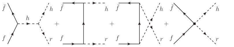
Figure 1: Feynman diagrams contributing to the asscociated Higgs boson-radion production in fermion-antifermion annihilation.

The corresponding contributions to the amplitude simplified using the Dirac equation and the identity $(\cancel{k}-m_{f})\,\frac{\cancel{k}+m_{f}}{k^{2}-m_{f}^{2}}=1$ have the following form

$$M^{(rh)}_{1}=\bar{v}^{r}(p_{1})\,\frac{-i\,m_{f}}{v}\,u^{s}(p_{2})\,\frac{i}{k_{h}^{2}-m_{h}^{2}}\,\frac{-i}{\Lambda_{r}}\,(-2k_{h}\,p_{h}+4m_{h}^{2})\,r(p_{r})\,h(p_{h})$$ (3)

$$\begin{split}M^{(rh)}_{2}=\bar{v}^{r}(p_{1})\,\frac{-i}{\Lambda_{r}}\,\left\{\frac{3}{2}\,[(\cancel{p}_{1}+m_{f})-(\cancel{k}-m_{f})]+m_{f}\right\}\,r(p_{r})\,i\,\frac{\cancel{k}+m_{f}}{k^{2}-m_{f}^{2}}\,i\,\frac{-m_{f}}{v}\,u^{s}(p_{2})\,h(p_{h})\\ =-i\,\bar{v}^{r}(p_{1})\,\frac{1}{\Lambda_{r}}\,\frac{m_{f}}{v}\,\left\{-\frac{3}{2}\,+m_{f}\,\frac{\cancel{k}+m_{f}}{k^{2}-m_{f}^{2}}\right\}\,r(p_{r})\,u^{s}(p_{2})\,h(p_{h})\end{split}$$ (4)

$$\begin{split}M^{(rh)}_{3}=\bar{v}^{r}(p_{1})\,i\,\frac{-m_{f}}{v}\,h(p_{h})\,i\,\frac{\cancel{k}^{\prime}+m_{f}}{{k^{\prime}}^{2}-m_{f}^{2}}\,\frac{-i}{\Lambda_{r}}\,\left\{\frac{3}{2}\,[(-\cancel{k}^{\prime}+m_{f})-(\cancel{p}_{2}\,-m_{f})]+m_{f}\right\}\\ r(p_{r})\,u^{s}(p_{2})\\ =-i\,\bar{v}^{r}(p_{1})\,\frac{1}{\Lambda_{r}}\,\frac{m_{f}}{v}\,\left\{-\frac{3}{2}\,+m_{f}\,\frac{\cancel{k}^{\prime}+m_{f}}{{k^{\prime}}^{2}-m_{f}^{2}}\right\}\,r(p_{r})\,u^{s}(p_{2})\,h(p_{h})\end{split}$$ (5)

$$M^{(rh)}_{4}=\bar{v}^{r}(p_{1})\,\frac{-i}{\Lambda_{r}}\,\frac{4m_{f}}{v}\,h(p_{r})\,r(p_{r})\,u^{s}(p_{2})\,=-i\,\bar{v}^{r}(p_{1})\,\frac{1}{\Lambda_{r}}\,\frac{m_{f}}{v}\,\left\{4\right\}\,r(p_{r})\,u^{s}(p_{2})\,h(p_{h})$$ (6)

For clarity one can modify (3) using the simple kinematics relation:

$$k_{h}=p_{h}+p_{r}\quad\Rightarrow\quad p_{h}=k_{h}-p_{r}$$ (7)

$$2k_{h}\,p_{h}=2(p_{h}+p_{r})\,p_{h}=(p_{h}+p_{r})^{2}+p_{h}^{2}-p_{r}^{2}=k_{h}^{2}+p_{h}^{2}-p_{r}^{2}=k_{h}^{2}+m_{h}^{2}-m_{r}^{2}$$ (8)

therefore

$$\frac{-(2k_{h}\,p_{h})+4m_{h}^{2}}{k_{h}^{2}-m_{h}^{2}}=\frac{-k_{h}^{2}-m_{h}^{2}+m_{r}^{2}+4m_{h}^{2}}{k_{h}^{2}-m_{h}^{2}}=-1+\frac{m_{r}^{2}+2m_{h}^{2}}{k_{h}^{2}-m_{h}^{2}}$$ (9)

So (3) can be rewritten as follows

$$M^{(rh)}_{1}=-i\,\frac{m_{f}}{\Lambda_{r}\,v}\,\bar{v}^{r}(p_{1})\,r(p_{r})\,h(p_{h})\,\left\{-1+\frac{m_{r}^{2}+2m_{h}^{2}}{k_{h}^{2}-m_{h}^{2}}\right\}\,u^{s}(p_{2})$$ (10)

It is easy to put (4), (5), (6) and (10) together and write down the total amplitude for the $f\bar{f}\rightarrow rh$ process

$$\begin{split}M^{(rh)}_{tot}=-i\,\frac{m_{f}}{\Lambda_{r}\,v}\,r(p_{r})\,h(p_{h})\,\bar{v}^{r}(p_{1})\,\left\{m_{f}\,\frac{\cancel{k}+m_{f}}{k^{2}-m_{f}^{2}}+m_{f}\,\frac{\cancel{k}^{\prime}+m_{f}}{{k^{\prime}}^{2}-m_{f}^{2}}-\frac{3}{2}-\frac{3}{2}+4-1\right.\\ \left.+\frac{m_{r}^{2}+2m_{h}^{2}}{k_{h}^{2}-m_{h}^{2}}\right\}\,u^{s}(p_{2})\end{split}$$ (11)

Now let us write down the contributions to the amplitude of the double Higgs boson production process $f\bar{f}\rightarrow hh$ (Fig.2) and compare the results:

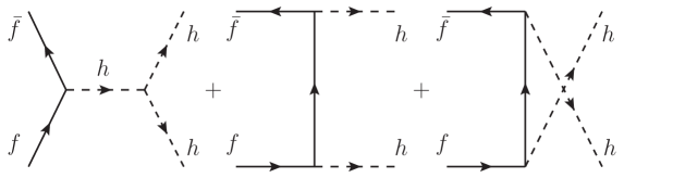
Figure 2: Feynman diagrams contributing to the double Higgs boson production in fermion-antifermion annihilation.

$$\begin{split}M^{(hh)}_{1}=\bar{v}^{r}(p_{1})\,i\frac{-m_{f}}{v}\,u^{s}(p_{2})\,\frac{i}{k_{h}^{2}-m_{h}^{2}}\,\frac{-i}{v}3m_{h}^{2}\,h(p_{h_{1}})\,h(p_{h_{2}})\\ =-i\frac{m_{f}}{v^{2}}\,h(p_{h_{1}})\,h(p_{h_{2}})\,\bar{v}^{r}(p_{1})\,\left\{\frac{3m_{h}^{2}}{k_{h}^{2}-m_{h}^{2}}\right\}\,u^{s}(p_{2})\end{split}$$ (12)

$$\begin{split}M^{(hh)}_{2}=\bar{v}^{r}(p_{1})\,i\frac{-m_{f}}{v}\,h(p_{h_{1}})\,i\frac{\cancel{k}+m_{f}}{k^{2}-m_{f}^{2}}\,i\frac{-m_{f}}{v}\,h(p_{h_{2}})\,u^{s}(p_{2})\\ =-i\frac{m^{2}_{f}}{v^{2}}\,h(p_{h_{1}})\,h(p_{h_{2}})\,\bar{v}^{r}(p_{1})\,\left\{\frac{\cancel{k}+m_{f}}{k^{2}-m_{f}^{2}}\right\}\,u^{s}(p_{2})\end{split}$$ (13)

$$\begin{split}M^{(hh)}_{3}=\bar{v}^{r}(p_{1})\,i\frac{-m_{f}}{v}\,h(p_{h_{2}})\,i\frac{\cancel{k^{\prime}}+m_{f}}{{k^{\prime}}^{2}-m_{f}^{2}}\,i\frac{-m_{f}}{v}\,h(p_{h_{1}})\,u^{s}(p_{2})\\ =-i\frac{m^{2}_{f}}{v^{2}}\,h(p_{h_{1}})\,h(p_{h_{2}})\,\bar{v}^{r}(p_{1})\,\left\{\frac{\cancel{k^{\prime}}+m_{f}}{{k^{\prime}}^{2}-m_{f}^{2}}\right\}\,u^{s}(p_{2})\end{split}$$ (14)

Notice that in this case there is no contribution like (6).

Thus, the total amplitude of the double Higgs production process yields

$$M^{(hh)}_{tot}=-i\,\frac{m_{f}}{v^{2}}\,h(p_{h1})\,h(p_{h2})\,\bar{v}^{r}(p_{1})\,\left\{m_{f}\,\frac{\cancel{k}+m_{f}}{k^{2}-m_{f}^{2}}+m_{f}\,\frac{\cancel{k}^{\prime}+m_{f}}{{k^{\prime}}^{2}-m_{f}^{2}}+\frac{3m_{h}^{2}}{k_{h}^{2}-m_{h}^{2}}\right\}\,u^{s}(p_{2})$$ (15)

Finally one can compare (11) and (15) and see the explicit cancellation of all the contributions that make the difference between the associated Higgs boson-radion and the double Higgs boson production.

In other words, (11) can be written in terms of (15) in the following way

$$M^{(rh)}_{tot}\sim\bar{v}^{r}(p_{1})\,\left\{m_{f}\,\frac{\cancel{k}+m_{f}}{k^{2}-m_{f}^{2}}+m_{f}\,\frac{\cancel{k}^{\prime}+m_{f}}{{k^{\prime}}^{2}-m_{f}^{2}}+\xi\frac{3m_{h}^{2}}{k_{h}^{2}-m_{h}^{2}}\right\}\,u^{s}(p_{2})$$ (16)

i.e, the expressions for the total amplitudes (11) and (15) coincide up to the replacements of the masses $m_{r}\rightarrow m_{h}$ and the denominators of the coupling constants $\Lambda_{r}\rightarrow v$ and to the renormalization of the triple Higgs coupling by the factor $\xi$, where

$$\xi\equiv 1+\frac{m_{r}^{2}-m_{h}^{2}}{3m_{h}^{2}}.$$

3 Associated Higgs boson-radion production in $gg$ fusion

As another example let us compare two processes involving gluons: the associated Higgs boson-radion production ($gg\rightarrow rh$) and the double Higgs boson production ($gg\rightarrow hh$), the corresponding diagrams are shown below.

One can see that the first four diagrams for the process of the radion production (Fig.3) are similar to those which appear in the SM (Fig.4). But the other three diagrams contain the Higgs boson-fermion-fermion-radion vertex which does not exist in the SM.

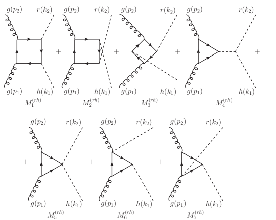
Figure 3: Feynman diagrams contributing to the associated Higgs boson-radion production ($gg\rightarrow rh$).

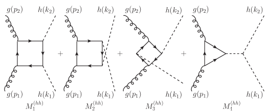
Figure 4: Feynman diagrams contributing to the double Higgs boson production ($gg\rightarrow hh$).

One can notice that all the contributions to the amplitudes of these processes have the following similar structure

$$M^{(rh)}_{i}=\frac{g_{c}^{2}}{v\,\Lambda_{r}}\,\epsilon(p_{1})_{\mu}\,\epsilon(p_{2})_{\nu}\,h(k_{1})\,r(k_{2})\,\int\frac{d^{d}l}{(2\pi)^{d}}\,X_{i}^{\mu\nu}(p_{1},p_{2},k_{1},k_{2})$$ (17)

for $gg\rightarrow rh$, where $i=1,2,...,7$;

$$M^{(hh)}_{i}=\frac{g_{c}^{2}}{v^{2}}\,\epsilon(p_{1})_{\mu}\,\epsilon(p_{2})_{\nu}\,h(k_{1})\,h(k_{2})\,\int\frac{d^{d}l}{(2\pi)^{d}}\,Y_{i}^{\mu\nu}(p_{1},p_{2},k_{1},k_{2})$$ (18)

for $gg\rightarrow hh$, where $i=1,2,3,4$;
where

$$X_{1}^{\mu\nu}\equiv Sp[\gamma^{\mu}\,S_{1}\,\gamma^{\nu}\,S_{2}\,\Gamma_{2,3}\,S_{3}\,(-m)\,S_{4}], Y_{1}^{\mu\nu}\equiv Sp[\gamma^{\mu}\,S_{1}\,\gamma^{\nu}\,S_{2}\,(-m)\,S_{3}\,(-m)\,S_{4}],$$

$$X_{2}^{\mu\nu}\equiv Sp[\gamma^{\mu}\,S_{1}\,\gamma^{\nu}\,S_{2}\,(-m)\,S_{5}\Gamma_{5,4}\,S_{4}], Y_{2}^{\mu\nu}\equiv Sp[\gamma^{\mu}\,S_{1}\,\gamma^{\nu}\,S_{2}\,(-m)\,S_{5}(-m)\,S_{4}],$$

$$X_{3}^{\mu\nu}\equiv Sp[\gamma^{\mu}\,S_{1}\,(-m)\,S_{6}\gamma^{\nu}\,S_{5}\,\Gamma_{5,4}\,S_{4}], Y_{3}^{\mu\nu}\equiv Sp[\gamma^{\mu}\,S_{1}\,(-m)\,S_{6}\gamma^{\nu}\,S_{5}\,(-m)\,S_{4}],$$

$$X_{4}^{\mu\nu}\equiv Sp[\gamma^{\mu}\,S_{1}\,\gamma^{\nu}\,S_{2}\,(-m)\,S_{4}]\,D\,\Gamma^{\prime}, Y_{4}^{\mu\nu}\equiv Sp[\gamma^{\mu}\,S_{1}\,\gamma^{\nu}\,S_{2}\,(-m)\,S_{4}]\,D\,\Gamma^{\prime},$$

$$X_{5}^{\mu\nu}\equiv Sp[\gamma^{\mu}\,S_{1}\,\gamma^{\nu}\,S_{2}\,(+4m)\,S_{4}],$$

$$X_{6}^{\mu\nu}\equiv Sp[\gamma^{\mu}\,S_{1}\,(-3\gamma^{\nu})\,S_{3}\,(-m)\,S_{4}],$$

$$X_{7}^{\mu\nu}\equiv Sp[(-3\gamma^{\mu})\,S_{1}\,\gamma^{\nu}\,S_{2}\,(-m)\,S_{5}],$$

and $\Gamma_{2,3}$, $\Gamma_{5,4}$, $\Gamma^{\prime}$ have the following form

$$\Gamma_{2,3}=\frac{3}{2}S_{2}^{-1}+\frac{3}{2}S_{3}^{-1}-m$$ (19)

$$\Gamma_{5,4}=\frac{3}{2}S_{5}^{-1}+\frac{3}{2}S_{4}^{-1}-m$$ (20)

$$\Gamma^{\prime}=\begin{cases}-3m_{h}^{2},\\ 2\left\{(k_{1}+k_{2})_{\mu}k_{1}^{\mu}-2m_{h}^{2}\right\}\end{cases}$$ (21)

The first line in (21) corresponds to the Higgs boson-fermion-fermion vertex in the $gg\rightarrow hh$ process and the second line – to the Higgs boson-radion-fermion-fermion vertex in the $gg\rightarrow rh$ process;

$$S_{j}^{-1}=(\cancel{l}-\cancel{q}_{j})-m,\quad D^{-1}=(k_{1}+k_{2})^{2}-m^{2},$$ (22)

$$q_{1}=0,\,q_{2}=-p_{2},\,q_{3}=-p_{2}+k_{2},\,q_{4}=-p_{2}+k_{2}+k_{1},\,q_{5}=-p_{2}+k_{1},\,q_{6}=k_{1}.$$

Let us notice that the radion-fermion-fermion vertex $\Gamma_{i,j}$ contains the inverse propagators $S_{i}^{-1}$ and $S_{j}^{-1}$. In the expressions $X_{1}^{\mu\nu}$, $X_{2}^{\mu\nu}$ and $X_{3}^{\mu\nu}$ for the box diagrams this vertex is surrounded by the propagators $S_{i}$ and $S_{j}$. This gives a reduction of a box diagram with the radion to a linear combination of two triangle diagrams and one box diagram with the vertex such as that of the Higgs boson as it is demonstrated in Fig.5.

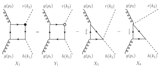
Figure 5: Reduction of a box diagram with the radion to a linear combination of one box diagram with the vertex such as that of the Higgs boson (the empty point) and two triangle diagrams.

This can be easily understood with the help of the tree-level illustration of a fermion current with emission of the radion, a gauge boson and the Higgs boson (Fig.6). The product of the radion-fermion-fermion vertex (the black point in Fig.6) and two propagators leads to three terms respectively:

$$S_{i}\,\Gamma_{i,j}\,S_{j}=S_{i}\,\left\{-m+\frac{3}{2}S_{j}^{-1}+\frac{3}{2}S_{i}^{-1}\right\}S_{j}$$

$$=-S_{i}\,m\,S_{j}+\frac{3}{2}\,S_{i}+\frac{3}{2}\,S_{j}$$

a Higgs-like term with the vertex proportional to the fermion mass (the empty point in Fig.6), a term with the $S_{j}$ propagator being dropped out, i.e., with the radion and the Higgs boson emission from the same point, and a term with the $S_{i}$ propagator being dropped out, with the radion and the gauge boson emission from the same point. In this way we get a reduction of each box diagram with the radion to a sum of other contributions.

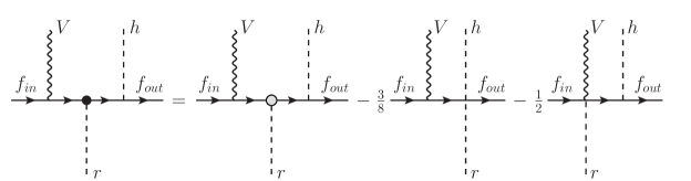
Figure 6: Fermion current with emission of the radion, a gauge boson and the Higgs boson expressed through the term with the Higgs-like vertex (the empty point) and two terms with four-point radion-boson vertices with corresponding numerical factors.

One can substitute (19)–(21) explicitly into the expressions $X_{i}^{\mu\nu}$ and open the brackets in order to get a representation of $X_{1}^{\mu\nu}$, $X_{2}^{\mu\nu}$ and $X_{3}^{\mu\nu}$ as sums of other $X_{i}^{\mu\nu}$ and $Y_{i}^{\mu\nu}$ contributions with the corresponding numerical factors

$$X_{1}^{\mu\nu}=Y_{1}^{\mu\nu}-\frac{3}{8}X_{5}^{\mu\nu}-\frac{1}{2}X_{6}^{\mu\nu}\\$$ (23)

$$X_{2}^{\mu\nu}=Y_{2}^{\mu\nu}-\frac{3}{8}X_{5}^{\mu\nu}-\frac{1}{2}X_{7}^{\mu\nu}\\$$ (24)

$$X_{3}^{\mu\nu}=Y_{3}^{\mu\nu}-\frac{1}{2}X_{6}^{\mu\nu}-\frac{1}{2}X_{7}^{\mu\nu}$$ (25)

The term $X_{4}^{\mu\nu}$ can be represented as a combination of $X_{i}^{\mu\nu}$ and $Y_{i}^{\mu\nu}$ contributions as follows

$$X_{4}^{\mu\nu}=-\frac{1}{4}X_{5}^{\mu\nu}+\frac{m_{r}^{2}+2m_{h}^{2}}{(k_{1}+k_{2})^{2}-m_{h}^{2}}Y_{4}^{\mu\nu}$$ (26)

by transforming the Higgs boson-radion vertex in the following way

$$\begin{split}\Gamma^{\prime}=2\left\{(k_{1}+k_{2})_{\mu}\,k_{1}^{\mu}-2m_{h}^{2}\right\}=(k_{1}+k_{2})^{2}+k_{1}^{2}-k_{2}^{2}-4m_{h}^{2}\\ =[(k_{1}+k_{2})^{2}-m_{h}^{2}]-m_{r}^{2}-2m_{h}^{2}\end{split}$$ (27)

and multiplying it by the propagator $D$ (22)

$$D\,\Gamma^{\prime}=1-\frac{m_{r}^{2}+2m_{h}^{2}}{(k_{1}+k_{2})^{2}-m_{h}^{2}}$$ (28)

Finally the sum of all $X_{i}^{\mu\nu}$ for the $gg\rightarrow rh$ process can be written in terms of $Y_{i}^{\mu\nu}$ and the parameter $\xi$ again as it has been done in the previous example (see (16))

$$\sum_{i=1}^{7}X_{i}^{\mu\nu}=Y_{1}^{\mu\nu}+Y_{2}^{\mu\nu}+Y_{3}^{\mu\nu}+\xi\,Y_{4}^{\mu\nu}$$ (29)

which looks very similar to the expression for the $gg\rightarrow hh$ process

$$\sum_{i=1}^{4}Y_{i}^{\mu\nu}=Y_{1}^{\mu\nu}+Y_{2}^{\mu\nu}+Y_{3}^{\mu\nu}+Y_{4}^{\mu\nu}$$ (30)

Thus, once again we see that the amplitudes for these two processes coincide up to the parameter $\xi$ and to the replacements of the masses and the denominators of the coupling constants.

One can notice that we could get the same amplitude if the model contains only the Higgs boson with renormalized parameters:

$$L=\frac{1}{2}\left(\partial_{\mu}h\right)\left(\partial^{\mu}h\right)-\frac{1}{2}m^{2}_{r}h^{2}-\frac{\xi}{2}\frac{m^{2}_{r}}{\Lambda_{r}}h^{3}+...$$ (31)

In other words, the radion contribution can mimic the deviation in the triple Higgs coupling. This fact must be taken into account in the investigation of $h^{3}$ coupling in the case of the radion detection. However this is valid only for the processes in the first order in the radion coupling constant, in more complicated cases the difference between the radion and the Higgs boson can be more significant and go beyond the simple replacement of the Higgs potential parameters.

4 Cancellations of additional to the Higgs-like contributions in associated Higgs boson-radion production

In paper [1] it was shown that all the additional contributions as compared to the Higgs boson case are cancelled out in the amplitudes of the single radion production processes. This property follows from the structure of any massive fermion current emitting the radion and an arbitrary number of any SM gauge bosons. Now let us show that the similar general property takes place in the case of the associated Higgs boson-radion production. Above we have already demonstrated the explicit cancellation by the example of the associated Higgs boson-radion production in fermion-antifermion annihilation and in gluon fusion. These were the processes with only two bosons ($rh$ or $hh$) in the final state. For the general proof let us consider a fermion current (or a fermion loop) with the emission of an arbitrary number, say $N$, of SM bosons (vector gauge – $V$ or Higgs – $h$) with all possible permutations. $N_{V}$ stands for the number of gauge bosons and $N_{h}$ – for the number of Higgs bosons, $N_{V}+N_{h}=N$. Now add another Higgs boson (for $f\bar{f}\rightarrow h_{1},...,h_{N_{h}+1},V_{1},...,V_{N_{V}}$) or another radion (for $f\bar{f}\rightarrow r,h_{1},...,h_{N_{h}},V_{1},...,V_{N_{V}}$) to this current in all possible ways.

There are two possibilities of adding a Higgs boson : a) the one emitted from the fermion line, and b) the one emitted from the boson ($V$ or $h$) line. For the radion there are the same options plus another one: c) the radion is emitted directly from the four-point vertex with $V$ or $h$ boson (Fig.7).

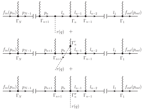
Figure 7: Fermion current radiating the radion and $N$ SM Higgs or vector gauge bosons, $l_{j}\equiv p_{j}-q$.

Let us first set the notations for all the vertices. For each vertex here all the lines are considered to be incoming. We will use Latin indices ($a,b,c$) for a parallel consideration of cases with gauge and Higgs bosons. In the case of gauge bosons the Latin indices take values of vector indices ($\alpha,\beta,\gamma,\mu$) and in the case of Higgs bosons they just reduce to the sign $(h)$ for Higgs boson vertices.

So, $\Gamma_{a}$ stands for the Lorentz part of the fermion-fermion-gauge boson vertex and for the fermion-fermion-Higgs boson vertex respectively

$$\Gamma_{a}=\begin{cases}\Gamma_{\mu}\\ \Gamma_{(h)}\end{cases}=i\begin{cases}\gamma_{\mu}\left(a_{f}+b_{f}\gamma_{5}\right)\\ -\frac{m_{f}}{v}\end{cases}$$ (32)

In the same manner we denote the vertex with two gauge bosons and the Higgs boson and the triple Higgs vertex

$$\left[\Gamma^{\prime}_{(h)}\right]^{a}_{b}=\begin{cases}\left[\Gamma^{\prime}_{(h)}\right]^{\alpha}_{\beta}\\ \Gamma^{\prime}_{(h)}\end{cases}=i\begin{cases}\frac{2m^{2}_{V}}{v}\delta^{\alpha}_{\beta}\\ -\frac{3m^{2}_{h}}{v}\end{cases}$$ (33)

Now for the radion, the fermion-fermion-radion vertex $\Gamma_{(r)}$ is a function of the momenta of the incoming fermions, say $p$ and $l$. It can be rewritten in terms of the inverse propagators $S^{-1}$ [1] and takes the following form

$$\begin{split}\Gamma_{(r)}(p,l)=-\frac{i}{\Lambda_{r}}\left\{\frac{3}{2}\left[(\cancel{p}+m_{f})-(\cancel{l}-m_{f})\right]+m_{f}\right\}\\ =\frac{i}{\Lambda_{r}}\left\{\frac{3}{2}\left[S^{-1}(l)+S^{-1}(-p)\right]-m_{f}\right\}\\ =\frac{v}{\Lambda_{r}}\Gamma_{(h)}+\frac{i3}{2\Lambda_{r}}\left[S^{-1}(l)+S^{-1}(-p)\right]\end{split}$$ (34)

The notation $\left[\Gamma^{\prime}_{(r)}\right]^{a}_{b}$ unifies the vertices for two gauge bosons and the radion interaction (excluding the anomalies) and for two Higgs bosons and the radion interaction respectively

$$\left[\Gamma^{\prime}_{(r)}\right]^{a}_{b}=\begin{cases}\left[\Gamma^{\prime}_{(r)}\right]^{\alpha}_{\beta}\\ \Gamma^{\prime}_{(r)}\end{cases}=i\begin{cases}\frac{2m^{2}_{V}}{\Lambda_{r}}\delta^{\alpha}_{\beta}\\ -\frac{2}{\Lambda_{r}}\left\{(p\cdot k)+2m^{2}_{h}\right\}\end{cases}$$ (35)

The term $\Gamma^{\prime\prime}_{(r),a}$ stands for gauge boson-fermion-fermion-radion and Higgs boson-fermion-fermion-radion four-point vertices

$$\Gamma^{\prime\prime}_{(r),a}=\begin{cases}\left[\Gamma^{\prime\prime}_{(r)}\right]_{\mu}\\ \Gamma^{\prime\prime}_{(r)}\end{cases}=\frac{i}{\Lambda_{r}}\begin{cases}3\gamma_{\mu}\left(a_{f}+b_{f}\gamma_{5}\right)\\ -\frac{4m_{f}}{v}\end{cases}=\frac{1}{\Lambda_{r}}\begin{cases}3\Gamma_{\mu}\\ 4\Gamma_{(h)}\end{cases}=\frac{3}{\Lambda_{r}}\Gamma_{a}+\frac{1}{\Lambda_{r}}\begin{cases}0\\ \Gamma_{(h)}\end{cases}$$ (36)

Now one can write down the contributions to the amplitudes in the following form

$$M[\varphi]_{n}=i^{N}\bar{f}(p_{out})\left[\prod_{j=1}^{n}\epsilon(k_{j})^{a_{j}}\Gamma_{a_{j}}S(p_{j}-q)\right]\varphi(q)\Gamma_{(\varphi)}\left[\prod_{j=n+1}^{N}S(p_{j-1})\epsilon(k_{j})^{a_{j}}\Gamma_{a_{j}}\right]f(p_{in})$$ (37)

$$\begin{split}M^{\prime}[\varphi]_{n}=i^{N}\bar{f}(p_{out})\left[\prod_{j=1}^{n-1}\epsilon(k_{j})^{a_{j}}\Gamma_{a_{j}}S(p_{j}-q)\right]\left(\epsilon(k_{n})^{a_{n}}\,\varphi(q)\,\left[\Gamma^{\prime}_{(\varphi)}\right]^{c}_{a_{n}}G(k_{n}+q)^{b}_{c}\,\Gamma_{b}\right)\times\\ \left[\prod_{j=n+1}^{N}S(p_{j-1})\epsilon(k_{j})^{a_{j}}\Gamma_{a_{j}}\right]f(p_{in})\end{split}$$ (38)

$$\begin{split}M^{\prime\prime}[\varphi]_{n}=i^{N-1}\bar{f}(p_{out})\left[\prod_{j=1}^{n-1}\epsilon(k_{j})^{a_{j}}\Gamma_{a_{j}}S(p_{j}-q)\right]\left(\epsilon(k_{n})^{a_{n}}\,r(q)\,\left[\Gamma^{\prime\prime}_{(r)}\right]_{a_{n}}\right)\times\\ \left[\prod_{j=n+1}^{N}S(p_{j-1})\epsilon(k_{j})^{a_{j}}\Gamma_{a_{j}}\right]f(p_{in})\end{split}$$ (39)

where $\varphi$ is either $h$ or $r$ in (37), (38) and only $r$ in (39); $\epsilon(k_{j})^{a_{j}}$ is either $\epsilon(k_{j})^{\mu_{j}}$ (for the gauge boson) or $h(k_{j})$ (for the Higgs boson); $G(k_{n}+q)^{b}_{c}$ is either $G(k_{n}+q)^{\beta}_{\gamma}$ (the gauge boson propagator) or $G(k_{n}+q)$ (the Higgs boson propagator);

$$p_{n-1}=p_{n}-k_{n},\quad p_{in}=p_{N},\quad p_{out}=p_{0}-q.$$

The number $n$ runs from $1$ to $N$ ($n=1,2,...,N$). In the case of real initial and final fermions one should take into account another amplitude

$$M[\varphi]_{0}=i^{N}\left[\prod_{j=1}^{N}\epsilon(k_{j})^{a_{j}}\right]\varphi(q)\bar{f}(p_{out})\Gamma_{(\varphi)}\left[\prod_{j=1}^{N}S(p_{j-1})\Gamma_{a_{j}}\right]f(p_{in})$$ (40)

If the added particle is the Higgs boson, the amplitude takes the form

$$M[h]_{0}=i^{N}\bar{f}(p_{out})h(q)\Gamma_{(h)}\left[\prod_{j=1}^{N}S(p_{j-1})\epsilon(k_{j})^{a_{j}}\Gamma_{a_{j}}\right]f(p_{in})$$ (41)

If the added particle is the radion, one can write the following amplitude

$$\begin{split}M[r]_{0}=\frac{v}{\Lambda_{r}}i^{N}\left[\prod_{j=1}^{N}\epsilon(k_{j})^{a_{j}}\right]r(q)\bar{f}(p_{out})\Gamma_{(h)}\left[\prod_{j=1}^{N}S(p_{j-1})\Gamma_{a_{j}}\right]f(p_{in})\\ +\frac{i3}{2\Lambda_{r}}i^{N}\left[\prod_{j=1}^{N}\epsilon(k_{j})^{a_{j}}\right]r(q)\bar{f}(p_{out})S^{-1}(p_{0})\left[\prod_{j=1}^{N}S(p_{j-1})\Gamma_{a_{j}}\right]f(p_{in})\\ =\frac{v}{\Lambda_{r}}M[h]_{0}+\frac{i3}{2\Lambda_{r}}i^{N}\left[\prod_{j=1}^{N}\epsilon(k_{j})^{a_{j}}\right]r(q)\bar{f}(p_{out})\left[\prod_{j=1}^{N}\Gamma_{a_{j}}S(p_{j})\right]\Gamma_{a_{N}}f(p_{in})\end{split}$$ (42)

where we used (34) and the equation of motion $\bar{f}(p_{out})S^{-1}(p_{out})=0$ ($p_{out}$ is the outgoing momentum).

Now let us take any number $n$, $n=1,...,N$. In the case of adding a Higgs boson the sum of all amplitudes for the chosen $n$ is

$$\begin{split}M[h]_{n}+M^{\prime}[h]_{n}=i^{N}\left[\prod_{j=1}^{N}\epsilon(k_{j})^{a_{j}}\right]h(q)\bar{f}(p_{out})\left[\prod_{j=1}^{n-1}\Gamma_{a_{j}}S(p_{j}-q)\right]\\ \times\left\{\Gamma_{a_{n}}S(p_{n}-q)\Gamma_{(h)}+\left[\Gamma^{\prime}_{(h)}\right]^{c}_{a_{n}}G(k+q)^{b}_{c}\,\Gamma_{b}\right\}\left[\prod_{j=n+1}^{N}S(p_{j-1})\Gamma_{a_{j}}\right]f(p_{in})\end{split}$$ (43)

For the case of adding a radion the sum has the following form

$$\begin{split}M[r]_{n}+M^{\prime}[r]_{n}+M^{\prime\prime}[r]_{n}=i^{N}\left[\prod_{j=1}^{N}\epsilon(k_{j})^{a_{j}}\right]r(q)\bar{f}(p_{out})\left[\prod_{j=1}^{n-1}\Gamma_{a_{j}}S(p_{j}-q)\right]\\ \times\left\{\Gamma_{a_{n}}S(p_{n}-q)\Gamma_{(r)}+\left[\Gamma^{\prime}_{(r)}\right]^{c}_{a_{n}}G(k+q)^{b}_{c}\,\Gamma_{b}-i\left[\Gamma^{\prime\prime}_{(r)}\right]_{a_{n}}\right\}\left[\prod_{j=n+1}^{N}S(p_{j-1})\Gamma_{a_{j}}\right]f(p_{in})\end{split}$$ (44)

One can calculate the part in curly brackets in (44) and compare it with that in (43)

$$\begin{split}\Gamma_{a_{n}}S(p_{n}-q)\Gamma_{(r)}+\left[\Gamma^{\prime}_{(r)}\right]^{c}_{a_{n}}G(k+q)^{b}_{c}\,\Gamma_{b}-i\left[\Gamma^{\prime\prime}_{(r)}\right]_{a_{n}}=\\ \frac{v}{\Lambda_{r}}\left(\Gamma_{a_{n}}S(p_{n}-q)\Gamma_{(h)}+\begin{Bmatrix}1\\ 1+\xi\end{Bmatrix}\left[\Gamma^{\prime}_{(h)}\right]^{c}_{a_{n}}G(k+q)^{b}_{c}\,\Gamma_{b}\right)\\ +\frac{i3}{2\Lambda_{r}}\Gamma_{a_{n}}(S(p_{n}-q)S^{-1}(p_{n})-1)\end{split}$$ (45)

Substituting the result (45) into expression (44) and opening the brackets one gets

$$\begin{split}M[r]_{n}+M^{\prime}[r]_{n}+M^{\prime\prime}[r]_{n}=i^{N}\left[\prod_{j=1}^{N}\epsilon(k_{j})^{a_{j}}\right]r(q)\bar{f}(p_{out})\left[\prod_{j=1}^{n-1}\Gamma_{a_{j}}S(p_{j}-q)\right]\\ \times\frac{v}{\Lambda_{r}}\left(\Gamma_{a_{n}}S(p_{n}-q)\Gamma_{(h)}+\begin{Bmatrix}1\\ 1+\xi\end{Bmatrix}\left[\Gamma^{\prime}_{(h)}\right]^{c}_{a_{n}}G(k+q)^{b}_{c}\,\Gamma_{b}\right)\left[\prod_{j=n+1}^{N}S(p_{j-1})\Gamma_{a_{j}}\right]f(p_{in})\\ +i^{N}\left[\prod_{j=1}^{N}\epsilon(k_{j})^{a_{j}}\right]r(q)\bar{f}(p_{out})\left[\prod_{j=1}^{n-1}\Gamma_{a_{j}}S(p_{j}-q)\right]\\ \times\frac{i3}{2\Lambda_{r}}\Gamma_{a_{n}}(S(p_{n}-q)S^{-1}(p_{n})-1)\left[\prod_{j=n+1}^{N}S(p_{j-1})\Gamma_{a_{j}}\right]f(p_{in})\end{split}$$ (46)

Here the first term has almost the same form as in the case of the Higgs boson (the absolute similarity would take place if $\xi=0$ and $v=\Lambda_{r}$). In the second term one can open the brackets and get

$$\begin{split}i^{N}\left[\prod_{j=1}^{N}\epsilon(k_{j})^{a_{j}}\right]r(q)\bar{f}(p_{out})\left[\prod_{j=1}^{n-1}\Gamma_{a_{j}}S(p_{j}-q)\right]\frac{i3}{2\Lambda_{r}}\Gamma_{a_{n}}(S(p_{n}-q)S^{-1}(p_{n})-1)\\ \times\left[\prod_{j=n+1}^{N}S(p_{j-1})\Gamma_{a_{j}}\right]f(p_{in})\\ =\frac{i3}{2\Lambda_{r}}i^{N}\left[\prod_{j=1}^{N}\epsilon(k_{j})^{a_{j}}\right]r(q)\bar{f}(p_{out})\left[\prod_{j=1}^{n}\Gamma_{a_{j}}S(p_{j}-q)\right]\Gamma_{a_{n+1}}\left[\prod_{j=n+2}^{N}S(p_{j-1})\Gamma_{a_{j}}\right]f(p_{in})\\ -\frac{i3}{2\Lambda_{r}}i^{N}\left[\prod_{j=1}^{N}\epsilon(k_{j})^{a_{j}}\right]r(q)\bar{f}(p_{out})\left[\prod_{j=1}^{n-1}\Gamma_{a_{j}}S(p_{j}-q)\right]\Gamma_{a_{n}}\left[\prod_{j=n+1}^{N}S(p_{j-1})\Gamma_{a_{j}}\right]f(p_{in})\\ =U_{n+1}-U_{n}\end{split}$$ (47)

where

$$U_{n}=\frac{i3}{2\Lambda_{r}}i^{N}\left[\prod_{j=1}^{N}\epsilon(k_{j})^{a_{j}}\right]r(q)\bar{f}(p_{out})\left[\prod_{j=1}^{n-1}\Gamma_{a_{j}}S(p_{j}-q)\right]\Gamma_{a_{n}}\left[\prod_{j=n+1}^{N}S(p_{j-1})\Gamma_{a_{j}}\right]f(p_{in})$$ (48)

for $n<N$.

It is easy to write $U_{1}$ in the following form

$$U_{1}=\frac{i3}{2\Lambda_{r}}i^{N}\left[\prod_{j=1}^{N}\epsilon(k_{j})^{a_{j}}\right]r(q)\bar{f}(p_{out})\left[\prod_{j=1}^{N-1}\Gamma_{a_{j}}S(p_{j})\right]\Gamma_{a_{N}}f(p_{in})$$ (49)

Getting back to the expression for $M[r]_{0}$ (42) one finds

$$M[r]_{0}=\frac{v}{\Lambda_{r}}M[h]_{0}+U_{1}$$ (50)

For $n=N$ one must separately consider the case of real initial and final fermions and the case of a fermion loop. For the first case the equation of motion $S^{-1}(p_{N})f(p_{in})=0$ is valid, thus

$$\begin{split}i^{N}\left[\prod_{j=1}^{N}\epsilon(k_{j})^{a_{j}}\right]r(q)\bar{f}(p_{out})\left[\prod_{j=1}^{N-1}\Gamma_{a_{j}}S(p_{j}-q)\right]\frac{i3}{2\Lambda_{r}}\Gamma_{a_{N}}(S(p_{N}-q)S^{-1}(p_{N})-1)\\ =-\frac{i3}{2\Lambda_{r}}i^{N}\left[\prod_{j=1}^{N}\epsilon(k_{j})^{a_{j}}\right]r(q)\bar{f}(p_{out})\left[\prod_{j=1}^{N-1}\Gamma_{a_{j}}S(p_{j}-q)\right]\Gamma_{a_{N}}f(p_{in})\\ =-U_{N}\end{split}$$ (51)

Finally for the case of real initial and final fermions we have

$$\begin{split}M[r]_{0}+\sum_{n=1}^{N}(M[r]_{n}+M^{\prime}[r]_{n}+M^{\prime\prime}[r]_{n})=\frac{v}{\Lambda_{r}}M[h]_{0}+\frac{v}{\Lambda_{r}}\sum_{n=1}^{N}\left(M[h]_{n}+\begin{Bmatrix}1\\ 1+\xi\end{Bmatrix}M^{\prime}[h]_{n}\right)\\ +U_{1}+(U_{2}-U_{1})+(U_{3}-U_{2})+\ldots+(U_{N}-U_{N-1})-U_{N}=\\ \frac{v}{\Lambda_{r}}M[h]_{0}+\frac{v}{\Lambda_{r}}\sum_{n=1}^{N}\left(M[h]_{n}+\begin{Bmatrix}1\\ 1+\xi\end{Bmatrix}M^{\prime}[h]_{n}\right)\end{split}$$ (52)

In the case of the fermion loop ($p_{in}=p_{out}$) one can move $\bar{f}(p_{out})$ by cyclic permutations to the end of the matrix product, which leaves the trace invariant, so $f(p_{in})\bar{f}(p_{out})=S(p_{in})=S(p_{out})$ and therefore $S^{-1}(p_{N})f(p_{in})\bar{f}(p_{out})=1$.

$$\begin{split}i^{N}\left[\prod_{j=1}^{N}\epsilon(k_{j})^{a_{j}}\right]r(q)\bar{f}(p_{out})\left[\prod_{j=1}^{N-1}\Gamma_{a_{j}}S(p_{j}-q)\right]\frac{i3}{2\Lambda_{r}}\Gamma_{a_{N}}(S(p_{N}-q)S^{-1}(p_{N})-1)f(p_{in})\\ =\frac{i3}{2\Lambda_{r}}i^{N}\left[\prod_{j=1}^{N}\epsilon(k_{j})^{a_{j}}\right]r(q)\left[\prod_{j=1}^{N}\Gamma_{a_{j}}S(p_{j}-q)\right]-U_{N}\end{split}$$ (53)

It is easy to check that the last but one term in (53) is equal to $U_{1}$. Indeed, it can be shown by means of the same trick: moving $f(p_{in})$ to the beginning and shifting the loop momentum by the value $q$. Thus, just as in the case of real fermions we get (52).

5 Conclusions

In the current work we have discussed the Higgs boson-radion similarity in their associated production processes. First, the associated Higgs boson-radion production was considered in two examples – in fermion-antifermion annihilation and gluon fusion. In both cases we have shown explicitly the Higgs boson-radion similarity up to the replacement of the masses and the denominators of the coupling constants and a rescaling of the triple Higgs coupling. Next, the general proof of this property was provided for the case of the radion production in association with an arbitrary number of the SM gauge or Higgs bosons. It was found that the Higgs boson-radion similarity in the considered types of processes does not allow us to distinguish a model with the radion and the Higgs boson from a model without the radion but with the Higgs boson with modified parameters. In particular, the radion contribution can mimic the deviation in the triple Higgs coupling. This fact must be taken into account in the investigation of $h^{3}$ coupling in the case of the radion detection.

Of course there exists the well-known difference between the radion and the Higgs boson because of the presence of the radion anomalous interaction. In addition to the enhancement of the radion decay modes to two gluons and to two photons the anomalous radion-gluon-gluon interaction contributes differently to the associated Higgs boson-radion and to the Higgs pair production. In the latter case the Higgs boson pair production may occur via the radion decay. The corresponding diagram does not participate in the cancellations and turns to a diagram of the same $\Lambda_{r}^{-1}$ order in the case of the resonant Higgs boson production ($m_{r}>2m_{h}$) while in the case of the non-resonant Higgs boson production ($m_{r}<2m_{h}$) this diagram is of the next order ($\Lambda_{r}^{-2}$). In fact, the anomalous radion-gluon-gluon interaction gives the leading contribution to the Higgs pair production via the radion decay.

The radion pair production is not considered in the current work being a model dependent and complicated study where the next orders ought to be taken into account.

It is important to mention that the considered property is valid not only for the radion in the brane-world models with two branes but it can also take place in scalar-tensor gravity theories (for example, the Brans-Dicke theory) or theories involving dilaton where the scalar field interacts with the trace of the energy-momentum tensor of matter.

6 Acknowledgments

The work was supported by grant 14-12-00363 of Russian Science Foundation. The authors are grateful to V. Bunichev, M. Smolyakov, and I. Volobuev for useful discussions and critical remarks.

References

[1]
E. Boos, S. Keizerov, E. Rakhmetov, K. Svirina,
Phys. Rev. D 90, 095026 (2014) [arXiv: 1409.2796 [hep-ph]].
[2]
L. Randall and R. Sundrum, Phys. Rev. Lett. 83, 3370
(1999) [arXiv:hep-ph/9905221].
[3]
W. D. Goldberger and M. B. Wise,
Phys. Lett. B 475, 275 (2000)
[hep-ph/9911457].
[4]
O. DeWolfe, D. Z. Freedman, S. S. Gubser and A. Karch,
Phys. Rev. D 62, 046008 (2000)
[hep-th/9909134].
[5]
C. Csaki, M. Graesser, L. Randall and J. Terning,
Phys. Rev. D 62, 045015 (2000)
[hep-ph/9911406].
[6]
C. Charmousis, R. Gregory and V. A. Rubakov,
Phys. Rev. D 62, 067505 (2000)
[hep-th/9912160].
[7]
C. Csaki, M. L. Graesser and G. D. Kribs,
Phys. Rev. D 63, 065002 (2001)
[hep-th/0008151].
[8]
E. E. Boos, Y. S. Mikhailov, M. N. Smolyakov and I. P. Volobuev,
Nucl. Phys. B 717, 19 (2005)
[hep-th/0412204].
[9]
E. E. Boos, Y. S. Mikhailov, M. N. Smolyakov and I. P. Volobuev,
Mod. Phys. Lett. A 21, 1431 (2006)
doi:10.1142/S0217732306020792
[hep-th/0511185].
[10]
G. F. Giudice, R. Rattazzi and J. D. Wells,
Nucl. Phys. B 595, 250 (2001)
[hep-ph/0002178];
[11]
K. -m. Cheung,
Phys. Rev. D 63, 056007 (2001)
[hep-ph/0009232];
[12]
G. D. Kribs,
eConf C 010630, P317 (2001)
[hep-ph/0110242];
[13]
M. Chaichian, A. Datta, K. Huitu and Z. -h. Yu,
Phys. Lett. B 524, 161 (2002)
[hep-ph/0110035].
[14]
T. G. Rizzo,
JHEP 0206, 056 (2002)
[hep-ph/0205242];
[15]
D. Dominici, B. Grzadkowski, J. F. Gunion and M. Toharia,
Nucl. Phys. B 671, 243 (2003)
[hep-ph/0206192];
[16]
J. F. Gunion, M. Toharia and J. D. Wells,
Phys. Lett. B 585, 295 (2004)
[hep-ph/0311219].
[17]
Z. Chacko, R. Franceschini and R. K. Mishra,
JHEP 1304, 015 (2013)
[arXiv:1209.3259 [hep-ph]];
[18]
Z. Chacko, R. K. Mishra and D. Stolarski,
JHEP 1309, 121 (2013)
[arXiv:1304.1795 [hep-ph]];
[19]
G. -C. Cho, D. Nomura and Y. Ohno,
Mod. Phys. Lett. A 28, 1350148 (2013)
[arXiv:1305.4431 [hep-ph]];
[20]
N. Desai, U. Maitra and B. Mukhopadhyaya,
JHEP 1310, 093 (2013)
[arXiv:1307.3765 [hep-ph]];
[21]
P. Cox, A. D. Medina, T. S. Ray and A. Spray,
JHEP 1402, 032 (2014)
[arXiv:1311.3663 [hep-ph]];
[22]
M. Geller, S. Bar-Shalom and A. Soni,
Phys. Rev. D 89, 095015 (2014)
[arXiv:1312.3331 [hep-ph]];
[23]
D. W. Jung and P. Ko,
Phys. Lett. B 732, 364 (2014)
[arXiv:1401.5586 [hep-ph]].
[24]
E. E. Boos, V. E. Bunichev, M. A. Perfilov, M. N. Smolyakov and I. P. Volobuev,
Phys. Rev. D 92, no. 9, 095010 (2015)
doi:10.1103/PhysRevD.92.095010
[arXiv:1505.05892 [hep-ph]].