Plasmons in QED Vacuum

Abstract

The problem of longitudinal oscillations of an electric field and a charge polarization density in QED vacuum is considered. Within the framework of semiclassical analysis, we calculate time-periodic solutions of bosonized (1+1)-dimensional QED (massive Schwinger model). Applying the Bohr–Sommerfeld quantization condition, we determine the mass spectrum of charge-zero bound states (plasmons) which correspond in quantum theory to the found classical solutions. We show that the existence of such plasmons does not contradict any fundamental physical laws and study qualitatively their excitation in (3+1)-dimensional real world.

I INTRODUCTION

It is a common knowledge that homogeneous plane electromagnetic waves in vacuum are transverse. The classical Maxwell equations in free space do not admit solutions which correspond to the longitudinal waves, i.e., waves with the electric- or magnetic-field vector collinear to the wave vector. Despite this well-known fact, in recent years a substantial degree of interest has been shown in various theoretical generalizations of Maxwell electrodynamics, which incorporate longitudinal waves, and in an experimental search for such waves in the radio frequency band van Vlaenderen and Waser (2001); Khvorostenko (1992); Podgainy and Zaimidoroga ; Monstein and Wesley (2002). However, it is clear that within the framework of the purely classical electrodynamics, any theoretical constructions of this type will lead to violation of the fundamental physical principles such as Lorentz invariance and the charge conservation law.

The situation changes in quantum electrodynamics (QED) due to virtual electron–positron pairs and vacuum polarization. Considering QED vacuum as a plasma of virtual electrons and positrons, one can suppose that longitudinal (Langmuir) oscillations should exist in such a medium. Continuing the analogy between the usual plasma and polarized vacuum, we can intuitively estimate possible characteristic frequencies of longitudinal oscillations of the electric field (plasmons) in QED as the frequencies comparable with the electron Compton frequency.

The nomenclature commonly accepted in QED refers to the fields described by the irrotational component of the four-potential as longitudinal waves Dirac (1966); Feynman (1949, 1998). It is known Feynman (1949), that such fields are nonphysical. However, this circumstance does not mean that longitudinal oscillations of an electric field cannot exist in principle. The problem of existence of longitudinal electric fields has direct bearing on the fundamental QED issue of an infinite electron self-energy, which is due to the instantaneous Coulomb interaction approach Feynman (1998). It is well known, that QED is a local theory in the sense that it considers interaction of point particles with an electromagnetic field, and the action within the framework of this theory is local. However, unlike the classical point electron, the Dirac electron possesses internal degrees of freedom, which are specified by the Dirac matrices. This leads to the quantum nonlocality effect discussed in, e.g., Efremov and Sharkov (2004, 2009). Allowance for such nonlocality on the Compton scales makes it possible to resolve the fundamental QED issue of an infinite electron self-energy. Obviously, the Coulomb law cannot be applicable at small distances of the order of the electron Compton wavelength. The Coulomb field, as a solution of the Maxwell equations, cannot satisfy exactly nonlinear QED equations of coupled electromagnetic and spinor fields. The influence of the nonlocality effects can be taken into account via modification of constitutive relations in Maxwell electrodynamics (effective nonlocal field theory) and, as will be shown below, leads to the possibility of longitudinal modes. The problem is thus related to the issues of causality and nonlocality in quantum theory, and is far from trivial.

Meanwhile, there is currently a great deal of interest in the dispersive vacuum effects Rozanov (1998); Grib et al. (1988); Gusynin and Shovkovy (1996); Dittrich and Gies (2000); Dunne (2004); Marklund and Shukla (2006); Lundin et al. (2006). Recent advances in the laser technology, such as the construction of powerful X-ray free electron lasers, make the fundamental effects related to the dispersive properties of quantum vacuum achievable in laboratory experiments Alkofer et al. (2001); Roberts et al. (2002); A. Di Piazza et al. (2006); Ruf et al. (2009); A. Di Piazza et al. (2012); P. Böhl et al. (2015). Thus, the poorly studied problem of existence of plasmons in QED vacuum is of not only theoretical, but also practical importance.

The well-known method of solving some complicated problems and obtaining nonperturbative results in quantum field theory suggests to treat the Heisenberg operator field equations as $c$-number field equations and find classical solutions to them. Some quantum properties can then be retrieved through semiclassical methods Dashen et al. (1974a, b); Jackiw (1977). We cannot apply this approach directly to the general QED equations of coupled electromagnetic and fermionic fields. While classical solutions of the purely Bose theory correspond to the coherent states of bosons, the classical limit of the Fermi fields, due to the exclusion principle and anticommutation relations, leads to some abstract construction with Grassmann numbers, the physical interpretation of which is challenging to obtain. However, the above-mentioned method can be applied to our problem if we limit ourselves to consideration only of one-space and one-time dimensions. In this case, we can bosonize QED, find time-periodic classical solutions, and then quantize these solutions using the Bohr–Sommerfeld quantization rule.

In this article, we present a simple semiclassical analysis of plasmons in quantum vacuum on the basis of bosonized QED in 1+1 dimensions, i.e., the massive Schwinger model Schwinger (1962); Coleman et al. (1975); Coleman (1976); Fischler et al. (1979); Adam (1996); Sadzikowski and Wegrzyn (1996); Byrnes et al. (2002); Nagy et al. (2004); Nandori (2011); Kleban et al. (2011). We describe a technique for calculating the spectra of plasmons and perform some qualitative study of their excitation in (3+1)-dimensional real world.

II BASIC EQUATIONS

The Lagrangian density of QED in 1+1 dimensions is given by Schwinger (1962); Coleman et al. (1975); Coleman (1976); Fischler et al. (1979)

$${\cal L}= i\bar{\psi}\gamma^{\mu}\partial_{\mu}\psi-g\bar{\psi}\gamma^{\mu}\psi A_{\mu}-m\bar{\psi}\psi$$ (1)

$$-{1\over 4}F^{\mu\nu}F_{\mu\nu}-{1\over 2}(\partial_{\mu}A^{\mu})^{2}.$$

The rationalized (Lorentz–Heaviside) natural units with $\hbar=c=1$ are employed and the following standard notations are used throughout: $\mu,\nu=0,1$, $x^{0}\equiv t$, $x^{1}\equiv x$, $\psi$ is a two-component spinor field, and the $\gamma$ matrices obey the relation $\gamma^{\mu}\gamma^{\nu}+\gamma^{\nu}\gamma^{\mu}=2{\rm g}^{\mu\nu}$ with the metric tensor ${\rm g}^{\mu\nu}={\rm diag}(1,-1)$. The Levi-Civita symbol is defined as $\varepsilon^{01}=-\varepsilon^{10}=1$. The electromagnetic field tensor $F_{\mu\nu}=\partial_{\mu}A_{\nu}-\partial_{\nu}A_{\mu}$, $g$ is a coupling constant with the dimension of mass, and $m$ is the bare mass of the electron.

The theory can be mapped into an equivalent Bose form via the bosonization rules Coleman et al. (1975); Coleman (1976); Fischler et al. (1979); Coleman (1975); Mandelstam (1975); Pogrebkov and Sushko (1975)

$${\cal N}_{m}[i\bar{\psi}\gamma^{\mu}\partial_{\mu}\psi]\rightarrow {1\over 2}{\cal N}_{\Lambda}(\partial_{\mu}\phi)^{2},$$

$${\cal N}_{m}[\bar{\psi}\gamma^{\mu}\psi]\rightarrow {1\over\sqrt{\pi}}\varepsilon^{\mu\nu}\partial_{\nu}\phi,$$

$${\cal N}_{m}[\bar{\psi}\psi]\rightarrow -{\exp(\gamma)\over 2\pi}{\Lambda}\,{\cal N}_{\Lambda}[\cos(2\sqrt{\pi}\phi)],$$ (2)

where $\Lambda=g/\sqrt{\pi}$, ${\cal N}_{\eta}$ denotes normal ordering with respect to the mass $\eta$ Coleman (1976), and $\gamma=0.577...$ is Euler’s constant. Applying relations (2), we will further consider the Bose fields $\phi$ and $A^{\mu}$ as $c$-number quantities. The classical limit of the bosonized version of Eq. (1) has the form

$${\cal L}= {1\over 2}(\partial_{\mu}\phi)^{2}-\Lambda\,\varepsilon^{\mu\nu}A_{\mu}\,\partial_{\nu}\phi+{a\over 2\pi}g\Lambda\,\cos(2\sqrt{\pi}\phi)$$ (3)

$$+{1\over 2}(F_{01})^{2}-{1\over 2}(\partial_{\mu}A^{\mu})^{2},$$

where $a=m\,\exp(\gamma)/g$. The field equations following from Lagrangian density (3) read

$$\square\phi+\Lambda E+a\pi^{-1}g^{2}\sin(2\sqrt{\pi}\phi)=0,$$ (4)

$$\square A^{\mu}=j^{\mu},$$ (5)

where $\square=\partial^{\mu}\partial_{\mu}$, $E=F_{01}$ is the electric field, and $j^{\mu}=\Lambda\,\varepsilon^{\mu\nu}\partial_{\nu}\phi$ is the polarization current. It is obvious from Eq. (5) that imposing the Lorentz gauge condition

$$\partial_{\mu}A^{\mu}=0$$ (6)

ensures the fulfilment of the charge conservation law $\partial_{\mu}j^{\mu}=0$. Constraint (6) also implies that $A^{\mu}$ can be written as $A^{\mu}=\varepsilon^{\mu\nu}\partial_{\nu}u$. Thus, from Eq. (5) we have

$$\partial_{\nu}(\square u-\Lambda\phi)=0.$$ (7)

Integrating Eq. (7) yields $\phi=\Lambda^{-1}\square u$ and

$$E=\square u=\Lambda\phi.$$ (8)

We restrict ourselves to consideration only of the case where the constant of integration for Eq. (7), known as the $\theta$ angle of the theory Coleman (1976), is zero. The case $\theta\neq 0$ corresponds to the appearance of a background electrostatic field Coleman (1976) and can also be of some physical interest. However, it should be noted that even a very small value of $\theta$ (in the natural units used in our work) corresponds actually to a giant (from the engineering viewpoint) electrostatic field. Thus, the choice $\theta=0$ seems more physically justified in the context of the studied problem.

Inserting Eq. (8) into Eq. (4) and introducing the dimensionless variables $\xi=\Lambda x$ and $\tau=\Lambda t$, we obtain

$$\partial^{2}_{\tau}\phi-\partial^{2}_{\xi}\phi+\phi+a\sin(2\sqrt{\pi}\phi)=0.$$ (9)

This is the massive sine-Gordon (MSG) equation Fischler et al. (1979); Sadzikowski and Wegrzyn (1996), i.e., bosonized version of (1+1)-dimensional QED.

It is the main purpose of the forthcoming analysis to find physically meaningful solutions of Eq. (9). In all the subsequent calculations, for modeling the polarization of electron–positron vacuum we adopt (see, e.g., Hebenstreit et al. (2013))

$$g/m=0.303\approx\sqrt{4\pi\alpha},$$ (10)

where $\alpha$ is the fine-structure constant ($a\approx 5.88$ in this case).

The potential energy for the scalar field $\phi$ is given by

$$V(\phi)={1\over 2}\phi^{2}-{a\over 2\sqrt{\pi}}\cos(2\sqrt{\pi}\phi).$$ (11)

The dependence $V(\phi)$ in the case (10) is shown in Fig. 1(a). It is seen that $V(\phi)$ possesses four stable classical minima. However, only one state $\phi=0$ is the true minimum corresponding to the stable state in quantum theory. The other three minima will be unstable when tunneling effects are taken into account Voloshin et al. (1975); S. Coleman (1977).

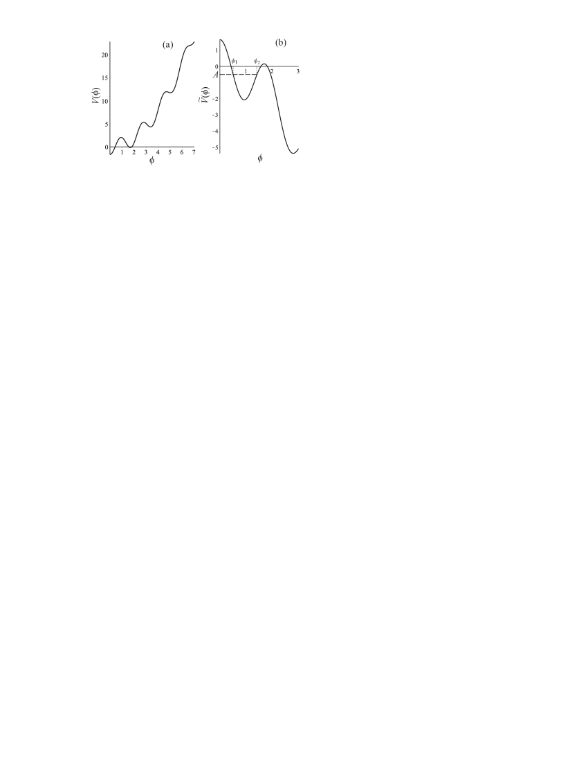
Figure 1: (a) The potential for the MSG equation (9) in the case (10) and (b) the inverted potential ${\tilde{V}}=-V$.

Let us consider briefly traveling wave solutions of Eq. (9), which are apparently the unique case where exact analytical results can be obtained. Substituting $\phi(\xi,\tau)=\phi(\eta)$, where $\eta=\xi-\beta\tau$ ($\beta<1$), into Eq. (9), after simple algebra we obtain

$$\left({d\phi\over d\eta}\right)^{2}={2\over 1-\beta^{2}}[A+V(\phi)],$$ (12)

where $A$ is an integration constant. This equation formally corresponds to the one-dimensional mechanical motion of a particle in an inverted potential ${\tilde{V}}=-V$. The oscillations between two values $\phi_{1}$ and $\phi_{2}$, where $\phi_{1}$ and $\phi_{2}$ are roots of the equation $A+V(\phi)=0$, are possible if $A+V(\phi)>0$ for $\phi_{1}<\phi<\phi_{2}$ [see Fig. 1(b)]. Thus, the MSG equation (9) admits periodic traveling wave solutions. The dispersion relation comprising the wavelength $\lambda$, the phase velocity $\beta$, and the amplitude $A$ is given by

$$\lambda=\sqrt{2}\sqrt{1-\beta^{2}}\int^{\phi_{2}}_{\phi_{1}}\frac{d\phi}{\sqrt{A+V(\phi)}}.$$ (13)

However, it can be shown that these solutions are modulationally unstable even in classical theory Whitham (1974). The instability will also occur in quantum theory due to the tunneling from one local minimum to another [see Fig. 1(b)]. In view of the above, we will not dwell on this case.

The problem of finding other solutions can be solved only with the help of numerical methods.

III STANDING WAVES AND SEMICLASSICAL QUANTIZATION

We will seek time-periodic solutions of the MSG equation (9) on the interval $|\xi|\leq L/2$. Let the solutions satisfy the boundary conditions

$$\phi(\xi=L/2,\tau)=\phi(\xi=-L/2,\tau)=0$$ (14)

and the time-periodicity condition

$$\phi(\xi,\tau+T)=\phi(\xi,\tau),$$ (15)

where $T=2\pi/\Omega$. The dimensional quantities $l$ and $\omega$, which correspond to conditions (14) and (15), are defined by $x/l=\xi/L$ and $\omega t=\Omega\tau$, respectively. Hence, $l\approx 5.85\,L/m$ and $\omega\approx 0.17\,\Omega\,m$.

It follows from Gauss’ law

$$\int^{L/2}_{-L/2}{\partial E\over\partial\xi}\,d\xi=\Lambda(\phi(L/2)-\phi(-L/2))=Q=0$$ (16)

that conditions (14) imply the zero total charge. Accordingly, the polarization current $j^{1}=-\partial_{t}E=-\Lambda\partial_{t}\phi$ vanishes at $\xi=\pm L/2$.

Before proceeding to numerical computations, let us give some elementary consideration concerning a weak field limit. The simplest solution of the linearized MSG equation (9), which satisfies conditions (14) and (15), i.e., the lowest linear normal mode, is given by

$$\phi(\xi,\tau)=A\,\cos(\pi\xi/L)\,\cos(\Omega\tau),$$ (17)

where

$$\Omega^{2}=\Omega^{2}_{0}=1+2a\sqrt{\pi}+\pi^{2}/L^{2}.$$ (18)

Observe that the minimum frequency of the linear oscillations is $\Omega_{0}(L=\infty)=(1+2a\sqrt{\pi})^{1/2}\approx 4.67$ ($\omega_{0}\approx 0.8\,m$). Let us suppose that solution (17) survives in the weakly nonlinear case. Taking into account the term proportional to $\phi^{3}$ in the series expansion of $\sin(2\sqrt{\pi}\phi)$, one can find an approximate amplitude correction to the dispersion relation (18):

$$\Omega^{2}=\Omega^{2}_{0}(L)-3a\pi^{3/2}A^{2}/4.$$ (19)

Equations (17)–(19) are useful for further analysis.

Any smooth solution of the boundary value problem that is specified by Eqs. (9) and (14) and periodic in time with the period $T$ has a Fourier representation. In our numerical calculations, we employ the Fourier pseudospectral algorithm Boyd (1986, 1990). It is convenient to seek the solution as the truncated Fourier series:

$$\phi(\xi,\tau)= \sum\limits^{M}_{m=1}\sum\limits^{N}_{n=1}\phi_{mn}\cos[(2m-1)\pi\xi/L]$$ (20)

$$\times\cos[(2n-1)\Omega\tau].$$

Due to the odd nonlinearity, no even harmonics will appear. In order to apply the iterative method, we write

$$\phi^{(i+1)}(\xi,\tau)=\phi^{(i)}(\xi,\tau)+\delta^{(i)}(\xi,\tau).$$ (21)

After linearization of Eq. (9) about the $i$th iterate $\phi^{(i)}$, we obtain

$$[\partial^{2}_{\tau}-\partial^{2}_{\xi}+1+2a\sqrt{\pi}\cos(2\sqrt{\pi}\phi^{(i)})]\delta^{(i)}$$

$$=\partial^{2}_{\xi}\phi^{(i)}-\partial^{2}_{\tau}\phi^{(i)}-\phi^{(i)}-a\sin(2\sqrt{\pi}\phi^{(i)}).$$ (22)

This equation is solved by expanding both $\phi^{(i)}$ and $\delta^{(i)}$ as double Fourier series similar to Eq. (20) and demanding that the left- and right-hand sides of Eq. (22) agree exactly at the $M\times N$ collocation points $\xi_{k}$ and $\tau_{j}$ such that $0<\xi_{k}<L/2$ and $0<\tau_{j}<T/2$, where $k=1,\ldots,M$ and $j=1,\ldots,N$. Equations (21) and (22) are iterated until $\delta^{(i)}$ is negligibly small. At each step, one has to find the Fourier coefficients $\delta^{(i)}_{mn}$ from the linear system of $M\times N$ equations (22).

The method has fast convergence and explicitly reveals periodicity of the desired solution. By means of this algorithm, we have built relatively simple and fast FORTRAN code. The possible computational problems inherent in the method are discussed in details in Boyd (1986). First, we must specify a sufficiently good guess for $\phi(\xi,\tau)$. Second, if the parameters $L$ and $\Omega$ in Eq. (20) are varied, the matrix of the linear system for the unknowns $\delta^{(i)}_{mn}$ will also vary, and one or more matrix eigenvalues may cross zero.

Our numerical strategy for computing periodic solutions is the following. We can fix the value of $L$ (say, $L=1$) and specify solution (17) with $A=1$ as the guess (i.e., $\phi^{(1)}_{11}=A$, while all the other coefficients $\phi^{(1)}_{mn}$ are equal to zero). In this case, setting $\Omega=\Omega_{0}(L)$ ensures that the iterations converge to the trivial solution, since Eq. (17) corresponds to the infinitesimally small values of $\phi$. Bearing Eq. (19) in mind and taking $\Omega\lesssim\Omega_{0}$, one can compute the Fourier coefficients for a finite-amplitude periodic solution. In all the computations, we use $M=N=15$, which gives high accuracy. It turns out that a small random shift of the collocation points from the nodes of the uniform grid improves convergence.

It is important that the correctness and possible computational errors of the solution can easily be checked with the help of standard mathematical software packages. Once the Fourier coefficients $\phi_{mn}$ in Eq. (20) have been obtained, we can determine what initial data $\varphi(\xi)=\phi(\xi,\tau=0)$ correspond to the found periodic solution. Imposing the initial conditions $\phi(\xi,0)=\varphi(\xi)$ and $\partial_{\tau}\phi(\xi,0)=0$ along with the boundary conditions (14), one can numerically integrate Eq. (9). We utilized the MAPLE intrinsic solver “pdsolve” for this purpose.

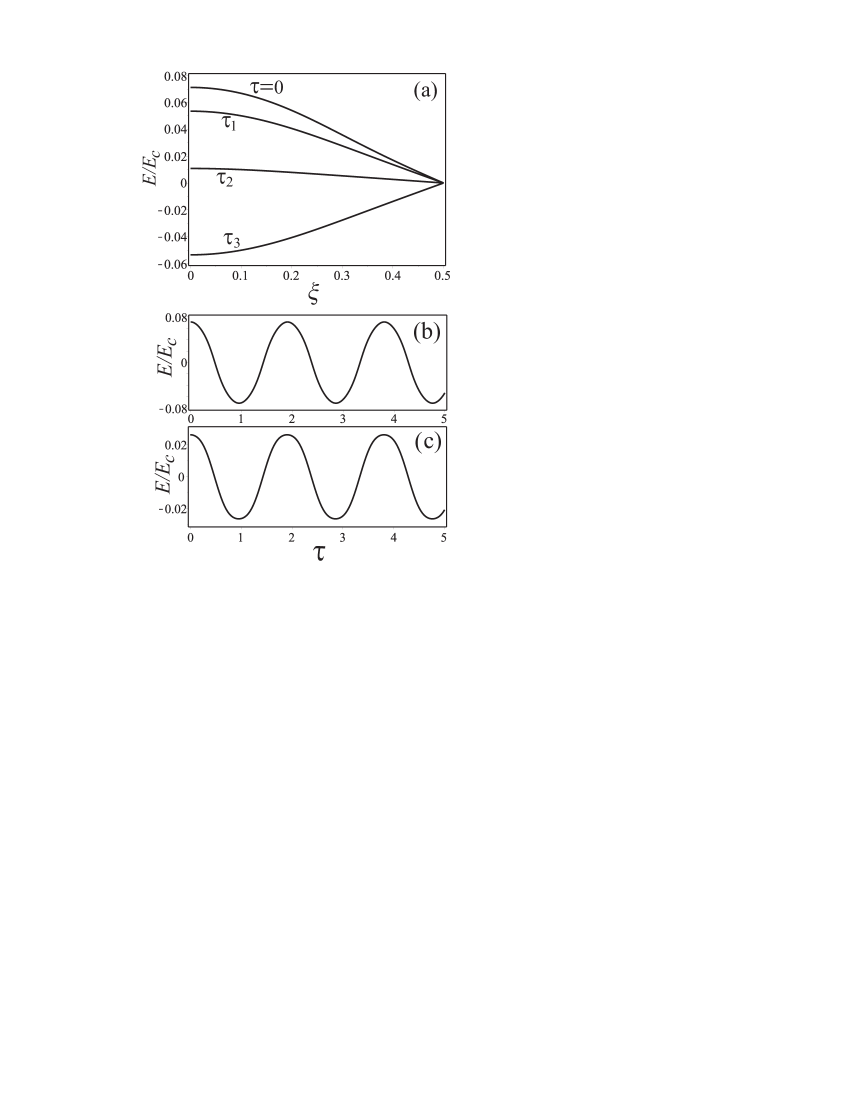
Figure 2: (a) Normalized electric field as a function of $\xi$ for $L=1$ ($l=5.85/m$) and $\Omega=3.3$ ($\omega=0.56\,m$) at time instants $\tau=0$, $\tau_{1}=\pi/(4\Omega)$, $\tau_{2}=0.46\pi/\Omega$, and $\tau_{3}=5\pi/(4\Omega)$. Oscillograms of the field at (b) $\xi=0$ and (c) $\xi=0.35$.

Figure 2(a) shows the snapshots of the normalized field

$$E/E_{c}=g^{2}\phi/(m^{2}\sqrt{\pi})$$ (23)

at fixed time instants for $L=1$ ($l=5.85/m$) and $\Omega=3.3$ ($\omega=0.56\,m$). Hereafter, $E_{c}=m^{2}/g$ is the critical Schwinger field strength. Figures 2(b) and 2(c) show the oscillograms of the field at the points $\xi=0$ and $\xi=0.35$, respectively. Although this case corresponds to the strong nonlinearity (the amplitude of the fundamental is $\phi_{11}=1.352$), the amplitudes of the higher harmonics are negligibly small (for example, $\phi_{12}=-0.053$ and $\phi_{21}=0.074$) and the oscillations turn out to be very close to monochromatic ones.

Fixing the quantity $L$ and consistently decreasing $\Omega$ from $\Omega_{0}(L)$ to smaller values, one can obtain an amplitude-frequency characteristic which is the dependence of the maximum field amplitude $E_{m}=E(0,0)$ of the time-periodic solution on the fundamental frequency $\Omega$. Figure 3 shows the amplitude-frequency characteristics for different values of $L$. It follows from the performed computations that for $L\lesssim 1.9$ ($l\lesssim 11/m$), the amplitude-frequency characteristics consist of four branches. Although the standing wave solutions have no direct analogy with a one-dimensional motion, the maximum field amplitudes for these branches approximately correspond to the minima of the potential $V(\phi)$ [see Fig. 1(a)].

Periodic solutions which correspond to the same $\Omega$ but different maximum amplitudes (different branches) can be calculated numerically by specifying different guess amplitude values. One should also note that once some solution (i.e., the set of $\phi_{mn}$) has been obtained, it can be used further as the guess itself.

The branches of the amplitude-frequency characteristics are connected at the bifurcation points, where $dE_{m}/d\omega=\infty$. At these points, the solution is not unique and iterative equation (22) is not soluble, since one or more matrix eigenvalues vanish Boyd (1986).

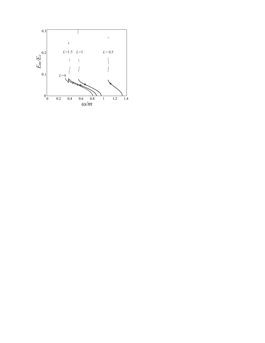
Figure 3: Amplitude-frequency characteristics for different values of $L$. The solution branches which correspond to the same $L$ and $\Omega$ but larger field amplitudes are shown by the dotted curves. The circles on the solid branches correspond to the values of $\Omega$ for which Eq. (26) is satisfied with $k=1$.

Figure 4(a) illustrates the mode shape which corresponds to the same parameters $L=1$ and $\Omega=3.3$ as for Fig. 2, but for the second branch in Fig. 3. The field oscillograms of this solution are presented in Figs. 4(b) and 4(c). It is seen in Fig. 4 that the nonlinear effects become more pronounced here than those for the first solution branch [see Fig. 2]. The main Fourier coefficients are $\phi_{11}=2.11$, $\phi_{12}=0.002$, and $\phi_{21}=0.262$. Note that periodic oscillations corresponding to the third and fourth solution branches, despite their largest amplitudes, are again close to monochromatic ones.

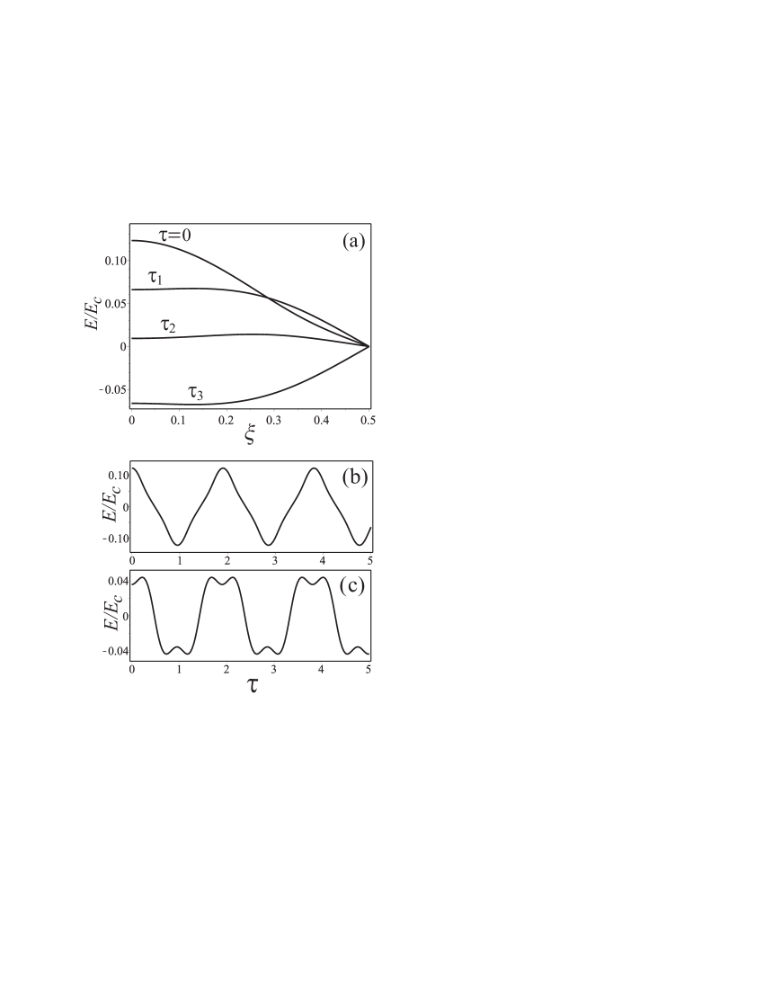
Figure 4: The same as in Fig. 2, but for the next solution branch.

The above-described picture of periodic solutions changes for $L\gtrsim 2$. For such values of $L$, we have found only single-branch amplitude-frequency characteristics. An example of such a characteristic is shown in Fig. 3 for $L=4$ ($l=23.4/m$). We can see that the characteristic for $L=4$ differs from other characteristics by the presence of small-amplitude spikes. The peaks of the spikes correspond to the singular points at which $dE_{m}/d\omega=\infty$. The appearance of these spikes is due to the resonances of the higher harmonics of the fundamental frequency inside our nonlinear “cavity resonator” with the “mirrors” at $\xi=\pm L/2$. Figures 5 and 6 illustrate how the mode shape changes when the fundamental frequency switches from $\Omega=2.3$ ($\omega=0.39\,m$) to $\Omega=2.2$ ($\omega=0.37\,m$) which is closer to the resonance. With increasing $L$, the number of the resonances increases, and overlapping of the resonances destroys a periodic solution. Our calculations show that for $L\gtrsim 5$, the existence of periodic solutions is a rare event.

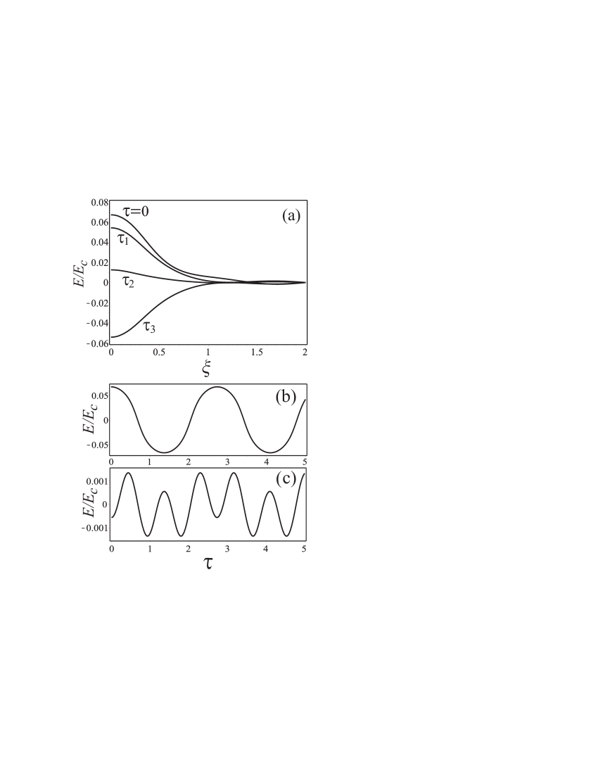
Figure 5: (a) Normalized electric field as a function of $\xi$ for $L=4$ ($l=23.4/m$) and $\Omega=2.3$ ($\omega=0.39\,m$) at time instants $\tau=0$, $\tau_{1}=\pi/(4\Omega)$, $\tau_{2}=0.46\pi/\Omega$, and $\tau_{3}=5\pi/(4\Omega)$. Oscillograms of the field at (b) $\xi=0$ and (c) $\xi=1.5$.

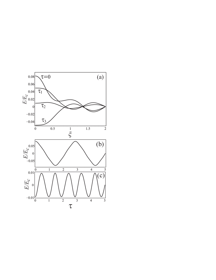
Figure 6: (a) Normalized electric field as a function of $\xi$ for $L=4$ ($l=23.4/m$) and $\Omega=2.2$ ($\omega=0.37\,m$) at time instants $\tau=0$, $\tau_{1}=\pi/(4\Omega)$, $\tau_{2}=0.46\pi/\Omega$, and $\tau_{3}=5\pi/(4\Omega)$. Oscillograms of the field at (b) $\xi=0$ and (c) $\xi=1.5$.

It is interesting to consider briefly some results of numerical integration for large $L$. Figure 7 illustrates two oscillograms of the solutions $\phi_{1}(\xi,\tau)$ and $\phi_{2}(\xi,\tau)$ of the boundary value problem specified by Eqs. (9) and (14) for $L=10$ with slightly different initial conditions

$$\phi_{1,2}(\xi,\tau=0)=A_{1,2}\cos(\pi\xi/10),$$

$$\partial_{\tau}\phi_{1,2}(\xi,\tau=0)=0,$$ (24)

where $A_{1}=5$ and $A_{2}=5.01$. As is seen in Fig. 7, a tiny difference in the initial conditions leads to a quite different time evolution. This test assumes the existence of chaotic dynamics and confirms the nonintegrability of the problem. Consequently, finding exact analytical solutions is a hopeless task.

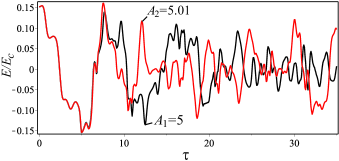
Figure 7: Results of numerical integration of Eq. (9) with the boundary conditions (14) for the initial conditions (24). The black and red curves correspond to the normalized field oscillograms at $\xi=3$ for the solutions with $A_{1}=5$ and $A_{2}=5.01$, respectively.

It should be emphasized that all the periodic solutions have been checked and an excellent agreement has been found between the pseudospectral (iterative) method and the calculations via MAPLE pdsolve in which a centered implicit scheme is employed. Under the given initial conditions, MAPLE yields the curves which are visually indistinguishable from those of the pseudospectral method on all the plots in Figs. 2 and 4–6. We have also analyzed the stability of periodic solutions. Namely, we have numerically integrated Eq. (9) with the boundary conditions (14) for the initial conditions which result from the mode shapes at $\tau=0$ and are augmented by small perturbations. This analysis, performed for a number of situations, furnishes a positive test for the overall robustness of the found standing wave solutions. The exceptions are the resonant modes whose parameters $\Omega$ and $L$ correspond to small neighborhoods of the spikes in Fig. 3. It is clear that small perturbations lead to destruction of periodic solutions in these cases. Thus, although the numerical tests are not a rigorous mathematical proof of stability, we can state that the nonsingular points ($dE_{m}/d\omega\neq\infty$) of the characteristics for $L\leq 1.5$ in Fig. 3 refer to the classically stable solutions. In quantum theory, however, one can expect the decay of the bound states which are related to the classical solutions corresponding to the dotted branches in Fig. 3. This is because the existence of such solutions is due to the false vacua of the potential [see Fig. 1(a)]. Our numerical computations also show that the periodic solutions which correspond to the true minimum of the potential $V$ [solid curves in Fig. 3] minimize the action, while the solutions labeled by the dotted curves correspond to the local maxima of the action functional.

The classical time-periodic solutions obtained above can be quantized via WKB methods Dashen et al. (1974a, b); Jackiw (1977). The Bohr–Sommerfeld quantization condition is written as

$$\int^{\pi/\Omega}_{0}\int^{L/2}_{-L/2}(\partial_{\tau}\phi)^{2}d\xi d\tau=k\pi,$$ (25)

where $k$ is a positive integer. Inserting Fourier representation (20) into Eq. (25), one obtains

$$\Omega L\sum\limits^{M}_{m=1}\sum\limits^{N}_{n=1}(2n-1)^{2}(\phi_{mn})^{2}=4k.$$ (26)

The coefficients $\phi_{mn}$ in Eq. (26) depend implicitly on $\Omega$ and $L$. Hence, for fixed $L$ the implicit equation (26) defines the masses of quantum states. The corresponding values of $\Omega$ for which Eq. (26) is satisfied with $k=1$ are shown in Fig. 3 by the circles on the solid branches. It is seen in Fig. 3 that the lowest masses (frequencies) and the related field strengths of quantum quasi-particles (plasmons), which are obtained from the quantization of the stable periodic solutions, are about $\omega\sim 0.5\,m$ and $E\sim 0.05\,E_{c}$, respectively. It is well known that in the general case, the Bohr–Sommerfeld condition is valid only for large $k$ ($k\gg 1$). Using the spatial periodicity of the found solutions, we can increase the length of the interval $|\xi|\leq L/2$ by an integer number of half periods $L$. Thus, with the replacement $L\to jL$, where $j$ is an arbitrary large integer, Eq. (26) will correctly define the mass spectrum of the bound states for $k\gg 1$. In classical theory, these states correspond to the periodic solutions (nonlinear normal modes E. Yu. Petrov and Kudrin (2010); Kudrin et al. (2016)) having a large number of field variations on the interval of length $jL$.

IV DISCUSSION

Feynman shows in his seminal work Feynman (1949), that the longitudinal waves for which $A_{\sigma}=\partial_{\sigma}\varphi$ are nonphysical. Indeed, the four-curl for these waves vanishes ($F_{\rho\sigma}=\partial_{\rho}\partial_{\sigma}\varphi-\partial_{\sigma}\partial_{\rho}\varphi=0$) and, accordingly, such a potential has no effect on a Dirac electron since the transformation $\psi^{\prime}=\exp(ig\varphi)\psi$, in the notation corresponding to our (1+1)-dimensional case, removes it. In our (1+1)-dimensional problem, we deal with the solenoidal divergence-free vector potential $A^{\mu}=\varepsilon^{\mu\nu}\partial_{\nu}u$. This field interacts with the spinor field and leads to the nonzero component $E_{x}(x,t)$ of the longitudinal electric field oscillations. Hence, our results do not contradict Feynman’s conjecture.

It follows from the performed analysis that periodic oscillations of the electric field, caused by oscillations of vacuum’s charge polarization density (collective excitations or plasmons of QED vacuum), can actually appear as solutions of the homogeneous (1+1)-dimensional QED equations without external sources. Probably, the most fundamental and complex question on the subject is what sources can excite such oscillations in real world. In what follows, we perform some qualitative analysis which gives evidence in favor of coupling the longitudinal oscillations and the transverse electromagnetic fields (photons) when the dispersive effects of polarized vacuum are taken into account. It should be emphasized that any effects of this kind can be observed, of course, only at very high field strengths that are expected to be created by powerful X-ray lasers.

Let us consider, for example, (3+1)-dimensional QED fields in the region between two perfectly conducting infinite plates located at $x=\pm l/2$ (Fabry–Perot resonator). For the low photon energy and a weak field, i.e.,

$$\omega\ll m,\quad|{\bf E}|\ll E_{c},\quad\omega/m\ll|{\bf E}|/E_{c},$$ (27)

one can employ the effective field theory approach represented by the Heisenberg–Euler Lagrangian with small dispersive corrections Rozanov (1998); Grib et al. (1988); Gusynin and Shovkovy (1996); Dittrich and Gies (2000); Dunne (2004); Marklund and Shukla (2006); Lundin et al. (2006). For simplicity, we will assume that the nonzero electromagnetic field components are $E_{x}(x,t)$, $E_{y}(x,t)$, and $B_{z}(x,t)$, for which ${\bf E}\cdot{\bf B}=0$. Vacuum polarization effects can be taken into account using the following modification of the constitutive relations in Maxwell’s theory:

$${\bf D}={\bf E}+{\hat{F}}(S,\square){\bf E},$$

$${\bf H}={\bf B}+{\hat{G}}(S,\square){\bf B},$$ (28)

where $S={\bf E}^{2}-{\bf B}^{2}$. If conditions (27) hold, one obtains Marklund and Shukla (2006); Lundin et al. (2006)

$${\hat{F}}={\hat{G}}={8\over 45}{\alpha^{2}\over m^{4}}S-{4\over 15}{\alpha\over m^{2}}\square.$$ (29)

Suppose now that $\omega$ approaches $m$. Then inequalities (27) are not satisfied and approximation (29) is not applicable. Nevertheless, due to the correspondence principle, coherent states of an electromagnetic field will still be described by the Maxwell equations with the constitutive relations (28). An explicit form of the operators ${\hat{F}}$ and ${\hat{G}}$ in this case is unknown at present. To ensure Lorentz invariance and the fundamental property that the traveling plane waves for which ${\bf E}^{2}={\bf B}^{2}$ and $\square{\bf E}=0$ do not polarize vacuum, these operators should depend only on the invariant $S$ and the wave operator $\square$. Hence, the equations for nonzero field components can be written as

$$\partial_{x}H_{z}=-\partial_{t}D_{y},$$ (30)

$$\partial_{x}E_{y}=-\partial_{t}B_{z},$$ (31)

$$\partial_{x}D_{x}=0.$$ (32)

It follows from Eqs. (30)–(32) that there exist degenerate nontrivial solutions for which $E_{x}\neq 0$, while all the other field components vanish and

$$D_{x}=E_{x}+{\hat{F}}(E^{2}_{x},\square)E_{x}=0.$$ (33)

There is a reason to believe that the operator ${\hat{F}}$ should be such that Eq. (33) will be equivalent or nearly equivalent to the MSG equation (9). This assumption is partially supported by the results of a recent work Lv et al. (2015). The authors of that work have examined the accuracy of an intrinsically (1+1)-dimensional QED to predict the forces and charges of a three-dimensional system that has a high degree of symmetry and therefore depends effectively only on a single spatial coordinate. There are no transverse electromagnetic waves or photons in (1+1)-dimensional QED (massive Schwinger model). However, as it has been shown in Lv et al. (2015), this model is not merely “a game of mind” and can correctly predict the vacuum polarization in a flat capacitor. The static electric displacements in (1+1)-dimensional and (3+1)-dimensional theories have been found to differ only slightly. Consequently, our assumption that the constitutive relations $D_{x}(E_{x})$ [see Eq. (33)] are nearly equivalent in both theories is supported by the results of Lv et al. (2015) in the static limit. Since the (3+1)-dimensional theory admits the time-dependent solutions in which there are no transverse electromagnetic fields and only the longitudinal electric field exists, it is natural to assume that these solutions can be described by an intrinsically (1+1)-dimensional QED, i.e., the corresponding time-dependent electric displacements are also nearly equivalent in both theories. To mathematically prove this assumption, one needs to find a nonperturbative explicit expression for the operator $\hat{F}$. This problem still remains unsolved at present.

In a more general case where the transverse (with respect to the $x$ direction) field components $E_{y}$ and $B_{z}$ are nonzero, it follows from Eqs. (30)–(31) that the equations for these components are coupled with Eq. (32). The coupling is due to the nonlinearity of relations (28), in which $S=E^{2}_{x}+E^{2}_{y}-B^{2}_{z}$. Thus, longitudinal oscillations can be excited by the transverse standing waves in the Fabry–Perot resonator at the frequencies $\omega\lesssim m$. The presence of longitudinal modes (plasmons in quantum theory) will affect counter-propagating photons and, hence, these modes cannot be ignored as nonphysical. It should also be noted that the magnetic-field component in such a hybrid longitudinal-transverse field configuration will significantly reduce the pair creation rate compared to the purely electric field case Ruf et al. (2009).

V CONCLUSIONS

In this article, we have studied the problem of plasmons in QED vacuum. It has been shown that the bosonized version of (1+1)-dimensional QED admits the existence of classical stable time-periodic solutions, i.e., standing waves of the longitudinal electric field and vacuum’s polarization density. We have numerically calculated mode shapes and field oscillograms for these solutions. The region of the existence of solutions in the parameter space has been established and numerical tests of their robustness have been performed. Applying the Bohr–Sommerfeld quantization condition, we have determined the mass spectrum of charge-zero bound states (plasmons) which correspond in quantum theory to the found classical solutions. We have also presented qualitative analysis which gives evidence in favor of coupling the longitudinal oscillations (plasmons) and the transverse waves (photons) in the dispersive vacuum. The performed analysis predicts the appearance of plasmons of QED vacuum in colliding laser pulses at the frequencies $\omega\sim 0.5\,m$. The required strength of the incoming laser field can be estimated as $E\geq 0.05\,E_{c}$. This can be relevant for future experiments with powerful X-ray and gamma lasers. To obtain a more precise estimate of the field strength, one needs to solve the (3+1)-dimensional problem with coupling between the longitudinal and transverse modes. However, the solution of this extremely hard problem falls beyond the scope of our article.