Deep Graphs - a general framework to represent and analyze heterogeneous complex systems across scales

Abstract

Network theory has proven to be a powerful tool in describing and analyzing systems by modelling the relations between their constituent objects. Particularly in recent years, great progress has been made by augmenting ‘traditional’ network theory in order to account for the multiplex nature of many networks, multiple types of connections between objects, the time-evolution of networks, networks of networks and other intricacies. However, existing network representations still lack crucial features in order to serve as a general data analysis tool. These include, most importantly, an explicit association of information with possibly heterogeneous types of objects and relations, and a conclusive representation of the properties of groups of nodes as well as the interactions between such groups on different scales. In this paper, we introduce a collection of definitions resulting in a framework that, on the one hand, entails and unifies existing network representations (e.g., network of networks, multilayer networks), and on the other hand, generalizes and extends them by incorporating the above features. To implement these features, we first specify the nodes and edges of a finite graph as sets of properties (which are permitted to be arbitrary mathematical objects). Second, the mathematical concept of partition lattices is transferred to network theory in order to demonstrate how partitioning the node and edge set of a graph into supernodes and superedges allows to aggregate, compute and allocate information on and between arbitrary groups of nodes. The derived partition lattice of a graph, which we denote by deep graph, constitutes a concise, yet comprehensive representation that enables the expression and analysis of heterogeneous properties, relations and interactions on all scales of a complex system in a self-contained manner. Furthermore, to be able to utilize existing network-based methods and models, we derive different representations of multilayer networks from our framework and demonstrate the advantages of our representation. On the basis of the formal framework described here, we provide a rich, fully scalable (and self-explanatory) software package that integrates into the PyData ecosystem and offers interfaces to popular network packages, making it a powerful, general-purpose data analysis toolkit. We exemplify an application of deep graphs using a real world dataset, comprising 16 years of satellite-derived global precipitation measurements. We deduce a deep graph representation of these measurements in order to track and investigate local formations of spatio-temporal clusters of extreme precipitation events.

The main focus of this paper is to provide a formal framework that enables a mathematically accurate description of any given system in a self-contained fashion. In addition, the purpose of this framework is to facilitate the utilization of existing methods and models supporting a practical data analysis. Network theory serves as the mathematical foundation of our framework. A network models the elements of a system as nodes, and their relations (or interactions) as edges. Particularly in the recent past – certainly also due to the deluge of available data – one could notice a large number of publications attempting to augment ‘traditional’ networks, in order to accommodate the increased heterogeneity of data, and to assign labels and values to nodes and edges (e.g. networks of networks, multilayer networks). The framework proposed here entails and unifies these approaches, but also generalizes them with two main aspects in mind: 1. Any node and any edge may be assigned possibly distinct types of properties (e.g., a node representing a human being may have ‘age’ as a type of property whose value is a number, and ‘blood values’ as another type of property whose value is a table of labels and numbers). 2. Integration of properties of groups of nodes and their respective interrelations within the same framework. Together, these objectives make it possible to combine different datasets (e.g., climatological and socioecological data or (electro)physiological records of different organs), integrate a priori knowledge of groups of objects and their relations, and carry out an analysis of potential relationships of the respective systems within the same network representation. On the basis of the mathematical work we provide here, existing network measures can be generalized and new measures developed. Yet, in order to practically conduct data analysis, we also provide a rich software implementation of our framework that integrates into the PyData ecosystem (which is comprised of various libraries for scientific computing), and offers interfacing methods to popular network packages, making it a considerable general-purpose data analysis toolkit.

I Introduction

At the present time, we are observing a quantification of our world at an unprecedented rate 90p . On the one hand – due to the rapid technological progress – we are extracting an ever increasing amount of information from nature, ranging from subatomic to astronomical scales. On the other hand, we are producing a vast amount of information in our daily lives interacting with electronic devices, thereby generating traceable information, tracked and stored by us personally, but also by organizations, companies and governments.

From a scientific point of view, this rapid increase in the amount and heterogeneity of available data poses both a great opportunity, but also methodological challenges: how can we describe and represent complex systems, made of multifarious subsystems interacting intricately on various scales; and once we have a suitable representation, how do we detect patterns and correlations, develop and test hypotheses and eventually come up with models and working theories of underlying mechanisms?

Thankfully, we can look back on centuries of scientific progress, tackling these questions. Rich tool sets to represent, analyze and model systems have been developed in various fields, such as: probability theory Jaynes (2005); multivariate statistics Anderson (2003); non-linear dynamics Strogatz (1994); Thiel et al. (2010); game theory Osborne and Rubinstein (1994); graph theory Newman (2010); or machine learning Hastie et al. (2009); Bishop (2006); Haykin (2009); Vapnik (1998); Deng and Yu (2014).

In this paper, we propose a framework that is capable of representing arbitrarily complex systems in a self-contained manner, and establishes an interface for the tools and methods developed in research disciplines such as those mentioned above. The framework is based on the ontological assumption that every system can be described in terms of its constituent objects (anything conceivable, i.e., “beings”, “things”, “entities”, “events”, “agents”, “concepts” or “ideas”) and their relations. With this assumption in mind, we build this framework based on graph or network theory. A graph, in its simplest form, is a collection of nodes (representing objects) where some pairs of nodes are connected by edges (representing the existence of a relation) Bollobas (1998). On top of that, we define an additional structure in order to meet the following objectives:

1. any node of the network may explicitly incorporate properties of the object(s) it represents. We refer to these properties as the features of a node, which themselves are mathematical objects.

2. any edge of the network may explicitly incorporate properties of the relation(s) it represents. We refer to these properties as the relations of an edge, which themselves are mathematical objects.

3. any subset of the set of all nodes of the network may be grouped into a supernode. Thereby, we may aggregate the features of the supernodes’ constituent nodes. Furthermore, we may allocate features particular to that supernode (“emergent” properties of the compound supernode), based on either the aggregated features, a priori knowledge, or both.

4. any subset of edges of the set of all edges of the network may be grouped into a superedge. Thereby, we may aggregate the relations of the superedges’ constituent edges. Furthermore, we may allocate relations particular to that superedge (“emergent” properties of the compound superedge), based on either the aggregated relations, a priori knowledge, or both.

5. we may place edges between any pair of supernodes, as well as between supernodes and nodes.

We believe that a comprehensive treatment of groups of objects, as well as their relations, is just as indispensable as an explicit incorporation of data, not only in the representation of complex systems, but also in their analysis. First, because it facilitates the means to represent features, relations and interactions on different scales, and second, because it allows us to coarse-grain, simplify and highlight important large-scale structures in a data-driven analysis.

Needless to say, this is not the first attempt to augment simple graphs in order to satisfy at least some of the above objectives. In weighted graphs, for instance, one can assign a number to each edge (i.e., the weight, strength, or distance of an edge) Horvath (2014). In node-weighted networks, it is possible to assign numbers to the nodes of the network Wiedermann et al. (2013). In hypergraphs, one can define edges joining more than two vertices at a time (called hyperedges), essentially allowing for the assignment of groups in a network Berge (1976). Such a membership of nodes in groups can also be represented by bipartite networks, where one of two kinds of nodes represents the original objects, and the other kind represents the groups to which the objects belong Asratian et al. (1998). Particularly in recent years – due to the deluge of available data – a multitude of frameworks has been proposed, with the aim of pluralizing the number of labels and values that may be assigned to a node, and allowing for different categories of connections between pairs of nodes, such as, e.g.: multivariate networks; multidimensional networks; interacting networks; interdependent networks; networks of networks; heterogeneous information networks; and multilayer networks (see Boccaletti et al. (2014); Kivelä et al. (2014); Berlingerio et al. (2011); Han (2012); De Domenico et al. (2013); Gao et al. (2011a, b); Santiago and Benito (2008) and references therein).

However, none of these frameworks satisfies all of the above objectives at the same time. In contrast, the framework proposed in this paper meets all these objectives. This allows us, on the one hand, to derive all of the above network representations as special cases by imposing certain constraints on our framework, which enables the utilization of the network-based methods, models and measures developed for them. On the other hand, we will demonstrate how the implementation of these objectives into our framework generalizes existing network representations, making it possible to combine heterogeneous datasets, integrate a priori knowledge of groups of objects and their relations, and conduct an analysis of potential interrelations of the respective systems within the same network representation. Considering the theoretical work provided here, existing network-measures may be generalized and new measures developed, particularly in respect of the heterogeneity of a system’s components and their interactions on different scales. Based on the introduced framework, we also provide a general-purpose data analysis software package dee that is fully scalable and integrates into the PyData ecosystem comprised of various libraries for scientific computing pyd . Apart from providing its own graph-theoretic data structure to accommodate the above objectives, our software package also provides interfaces for known data structures such as adjacency lists, adjacency matrices, incidence matrices and tensors, which have recently been introduced to represent multilayer networks De Domenico et al. (2013).

The paper is structured as follows: the theoretical part of our framework is described in Sec. II, where we introduce our representation of a graph, and Sec. III, where we demonstrate a comprehensive manner of graph partitioning. Thereafter, we outline the general procedure of constructing a deep graph and demonstrate how our framework integrates with existing data analysis tools in Sec. IV. We then demonstrate a real world application of our framework on a global precipitation dataset in Sec. V, before we draw our conclusions in Sec. VI.

II Graph Representation

Throughout this paper, we assume (w.l.o.g.) that (super)nodes, (super)edges, types of features and types of relations are represented by consecutive integers starting from 1. Also, there is a glossary in Tab. 4, which summarizes all the important quantities of a deep graph.

The basis of our representation is a finite, directed graph (possibly with self loops), given by a pair

$$G=(V,E),$$ (1)

where $V$ is a set of $n:=|V|$ nodes,

$$V=\{V_{i}\;\vline\;i\in\{1,2,...,n\}\},$$ (2)

and $E$ is a set of $m:=|E|$ directed edges, given by

$$E\subseteq\{E_{ij}\;\vline\;i,j\in\{1,2,...,n\}\}=:E^{\prime}.$$ (3)

Every node $V_{i}\in V$ of this graph represents some object(s), and every edge $E_{ij}\in E$ represents the existence of some relation(s) from node $V_{i}$ to node $V_{j}$. We say that an edge $E_{ij}$ is incident to both nodes $V_{i}$ and $V_{j}$. In order to explicitly incorporate information or data of the objects and their pairwise relations, we specify every node $V_{i}$ and every edge $E_{ij}$ of $G$ as a set of its respective properties. We refer to the properties of a node as its features, and to the properties of an edge as its relations.

Hence, we define every node $V_{i}$ as a set of $f_{i}$ features (and its index, to guarantee uniqueness of the nodes), given by

$$V_{i}=\{i,F_{i}^{1},F_{i}^{2},...,F_{i}^{f_{i}}\}.$$ (4)

As opposed to the ‘weight’ of a node in node-weighted networks Wiedermann et al. (2013) – which is usually a real number – a feature $F_{i}^{j}$ can be any mathematical object (e.g. numbers; quantitative or categorical variables; sets; matrices; tensors; functions; nodes; edges; graphs; but also strings to represent abstract objects, such as concepts or ideas). Furthermore, we associate every feature with a type, in order to express the kind of property a feature is related to and to establish a comparability between the features of different nodes. For example, for a node representing a city, some types of features might be ‘location’, ‘age’, ‘number of inhabitants’, ‘unemployment rate’ and ‘voting patterns’. For a node representing a neuron, some types of features could be ‘time series of the membrane potential’, ‘measuring device’ and ‘distribution of ion channel types’. On that account, we denote with $F=\{F^{j}_{i}\;\vline\;i\in\{1,2,...,n\}\land j\in\{1,2,...,f_{i}\}\}$ the set of all features, and with $T_{v}=\{1,2,...,n_{\text{types}}\}$ the set of all distinct types of features contained in the graph $G$. We then define a surjective function mapping every feature to its corresponding type,

$$t_{v}:F\rightarrow T_{v},F^{j}_{i}\mapsto t_{v}(F^{j}_{i}):=T^{j}_{i}\in T_{v},$$ (5)

such that $t_{v}(F^{j}_{i})=t_{v}(F^{l}_{k})$ for all pairs of features that share the same type. However, we do not allow a node $V_{i}$ to have multiple features of the same type, $t_{v}(F^{j}_{i})\neq t_{v}(F^{k}_{i})$ for all $j\neq k\in\{1,2,...,f_{i}\}$. In other words, every node $V_{i}$ has exactly $f_{i}$ distinct types of features. Figure 1(a) depicts different nodes along with their features and the feature’s types.

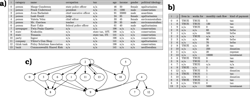
Figure 1: Graph Representation. Illustration of a fictional graph $G=(V,E)$ consisting of $n=14$ nodes and $m=22$ directed edges. (a) Representation of the nodes $V_{i}\in V$. The left column indicates the nodes’ indices, the top row indicates the types of features. A feature denoted “n/a” means that the corresponding node does not have a feature of the corresponding type. (b) Representation of the edges $E_{ij}\in E$. The first two columns from the left indicate the indices of edges $E_{ij}$ from node $V_{i}$ to node $V_{j}$ and the top row indicates the types of relations. A relation denoted “n/a” means that the corresponding edge does not have a relation of the corresponding type. (c) Depiction of the graph’s topology, where nodes are represented by indexed circles and edges are represented by arrows.

Analogously, we define every edge $E_{ij}\in E$ as a set of $r_{ij}$ relations (and its index pair, to guarantee uniqueness of the edges), given by

$$E_{ij}=\{(i,j),R_{ij}^{1},R_{ij}^{2},...,R_{ij}^{r_{ij}}\}.$$ (6)

Again, as opposed to the commonly real-valued ‘weight’ of an edge in edge-weighted networks Horvath (2014), a relation $R_{ij}^{k}$ can be any mathematical object. Just like features, we map every relation to its corresponding type, indicating the kind of property of a relation (e.g. ‘distance between’, ‘correlation between’, ‘similarity between’, ‘works for’, ‘is part of’). We denote with $R=\{R^{k}_{ij}\;\vline\;i,j\in\{1,2,...,n\}\land k\in\{1,2,...,r_{ij}\}\}$ the set of all relations, and with $T_{e}=\{1,2,...,m_{\text{types}}\}$ the set of all distinct types of relations contained in the graph $G$. We then map every relation onto a type,

$$t_{e}:R\rightarrow T_{e},R^{k}_{ij}\mapsto t_{e}(R^{k}_{ij}):=T^{k}_{ij}\in T_{e},$$ (7)

such that $t_{e}(R^{k}_{ij})=t_{e}(R^{l}_{mn})$ for all pairs of relations that share the same type, and $t_{e}(R^{k}_{ij})\neq t_{e}(R^{l}_{ij})$ for all $k\neq l\in\{1,2,...,r_{ij}\}$. Therefore, every edge $E_{ij}$ has exactly $r_{ij}$ distinct types of relations. Figure 1(b) illustrates several edges with different types of relations.

For notational convenience later on, we define all elements $E_{ij}\in E^{\prime}$ that are not in $E$ as empty sets,

$$E_{ij}:=\varnothing\text{ for all }i,j\in\{1,2,...,n\}:E_{ij}\in E^{\prime}\setminus E.$$ (8)

In other words, we say an edge from node $V_{i}$ to node $V_{j}$ exists if $E_{ij}\neq\varnothing$, and in this context, we term $V_{i}$ the source node and $V_{j}$ the target node. Therefore, we can rewrite the set of edges of $G=(V,E)$ as

$$E=\{E_{ij}\;\vline\;i,j\in\{1,2,...,n\}\land E_{ij}\neq\varnothing\}.$$ (9)

III Graph Partitioning

In this section, we introduce a comprehensive concept of graph partitioning. To avoid confusion: we do not refer to graph partitioning in the sense of finding “good” partitions (i.e. communities) based on some cost function or statistical measures Buluç et al. (2013) such as, e.g., Newman’s modularity measure Newman and Girvan (2004). Instead, we refer to graph partitioning in the more general sense of partitions of sets Lucas (1990).

First, we demonstrate how partitioning the node set $V$ of a graph $G=(V,E)$ enables us to group arbitrary nodes into supernodes, and equivalently, how partitioning the edge set $E$ allows us to group arbitrary edges into superedges. Then, we introduce a coherent manner of partitioning a graph $G=(V,E)$ into a supergraph, where the edge set $E$ is partitioned in accordance with a given partition of the node set $V$, based on the edges’ incidences to the nodes.

Partitioning nodes, edges or graphs – as we will show – not only conserves the information contained in the graph $G=(V,E)$, but allows us to redistribute it. This enables us to aggregate the features and relations of any desirable group of nodes and edges, and to allocate information particular to them. Furthermore, it facilitates the means to place edges between any supernodes or between supernodes and nodes, allowing us to represent interactions or relations on any scale of a complex system.

III.1 Partitioning Nodes

Given a graph $G=(V,E)$ with $n=|V|$ nodes, we define a surjective function mapping every node $V_{i}\in V$ to a supernode label (i.e. feature) ${}^{v}S_{i}$,

$${}^{v}p:V\rightarrow{}^{v}S=\{1,2,...,n^{p}\},V_{i}\mapsto{}^{v}p(V_{i}):={}^{v}S_{i}\in{}^{v}S.$$ (10)

This function induces a partition $V^{p}$ of $V$ into $n^{p}=|V^{p}|$ supernodes $V^{p}_{i}$, given by

$$V^{p}_{i}=\{V_{j}\;\vline\;j\in\{1,2,...,n\}\wedge{}^{v}p(V_{j})={}^{v}S_{i}\},\text{ and}$$ (11)

$$V^{p}=\{V^{p}_{i}\;\vline\;i\in\{1,2,...,n^{p}\}\}.$$ (12)

The number of nodes a supernode $V^{p}_{i}\in V^{p}$ contains is denoted by $n^{p,i}:=|V^{p}_{i}|\geq 1$.

The supernode labels given by the function ${}^{v}p(V_{i})={}^{v}S_{i}$ can be transferred as features to the nodes of $G$,

$$V_{i}=\{i,F^{1}_{i},F^{2}_{i},...,F^{f_{i}}_{i},{}^{v}S_{i}\},$$ (13)

where the type of feature of ${}^{v}S_{i}$ is the same for all nodes, $t_{v}({}^{v}S_{i})=t_{v}({}^{v}S_{j})$ for all $i,j\in\{1,2,...,n\}$. In turn, every feature itself can be interpreted as a supernode label, and we can say that its corresponding type induces a partition of the node set. For instance, looking at Fig. 1(a), we see that the type of feature ‘political ideology’ induces a partition of $V$ into $n^{p}=5$ supernodes: ‘egalitarianism’ (consisting of $n^{p,1}=4$ nodes), ‘conservatism’ ($n^{p,2}=6$ nodes), ‘anarchism’ ($n^{p,3}=1$ node), ‘environmentalism’ ($n^{p,4}=2$ nodes) and ‘neoliberalism’ ($n^{p,5}=1$ node). Since some nodes might not have a feature of a certain type [see for instance the type ‘gender’ in Fig. 1(a)], there is a degree of freedom when partitioning by that type: we can create one supernode comprising all nodes without the feature; create a separate supernode for every node without the feature; or create no supernode at all for these nodes. This choice is of course dependent on the analysis.

III.2 Partitioning Edges

Partitioning the edge set $E$ of a given graph $G=(V,E)$ with $n=|V|$ nodes and $m=|E|$ edges can be realized just like partitioning the node set. However, since edges $E_{ij}$ are incident to pairs of nodes $(V_{i},V_{j})$, we later demonstrate how to exploit this association in order to partition edges based on properties of the nodes. Here, we demonstrate the procedure analogous to that of partitioning nodes. Hence, we define a surjective function mapping every edge $E_{ij}\in E$ to a superedge label (i.e. relation) ${}^{e}S_{r}$, given by

$${}^{e}p:E\rightarrow{}^{e}S=\{1,2,...,m^{p}\},E_{ij}\mapsto{}^{e}p(E_{ij}):={}^{e}S_{r}\in{}^{e}S.$$ (14)

This function induces a partition $E^{p}$ of $E$ into $m^{p}=|E^{p}|$ superedges $E^{p}_{r}$, where

$$E^{p}_{r}=\{E_{uv}\;\vline\;\Phi^{e}(u,v)\land{}^{e}p(E_{uv})={}^{e}S_{r}\},$$ (15)

$$\Phi^{e}(u,v):(u,v\in\{1,2,...,n\}\land E_{uv}\neq\varnothing),\text{ and}$$ (16)

$$E^{p}=\{E^{p}_{r}\;\vline\;r\in\{1,2,...,m^{p}\}\}.$$ (17)

The number of edges a superedge $E^{p}_{r}\in E^{p}$ contains is denoted by $m^{p,r}:=|E^{p}_{r}|\geq 1$.

Equivalently to supernode labels, we can transfer the superedge labels given by the function ${}^{e}p(E_{ij})={}^{e}S_{r}$ as relations to the edges of $G$,

$$E_{ij}=\{(i,j),R^{1}_{ij},R^{2}_{ij},...,R^{r_{ij}}_{ij},{}^{e}S_{r}\},$$ (18)

where the type of relation of ${}^{e}S_{r}$ is the same for all edges, $t_{e}({}^{e}S_{i})=t_{e}({}^{e}S_{j})$ for all $i,j\in\{1,2,...,m\}$. Again, every relation itself can be interpreted as a superedge label, and we say that its corresponding type induces a partition of the edge set. Looking at Fig. 1(b), we see that the type of relation ‘kind of payment’ induces a partition of $E$ into $m^{p}=6$ superedges: ‘bribe’ (consisting of $m^{p,1}=4$ edges), ‘donation’ ($m^{p,2}=3$ edges), ‘expense’ ($m^{p,3}=1$ edge), ‘investment’ ($m^{p,4}=2$ edges), ‘tax’ ($m^{p,5}=10$ edges), and ‘n/a’ ($m^{p,6}=2$ edges). Since the last two edges do not have a relation of the type ‘kind of payment’, we could have also partitioned the edges into $m^{p}=5$ superedges (leaving the two edges out), or into $m^{p}=7$ superedges (the two edges are put into separate superedges).

III.3 Partitioning a Graph

Here, we introduce a coherent manner of partitioning a graph $G=(V,E)$ with $n=|V|$ nodes and $m=|E|$ edges, based on the edges’ incidences to the nodes. Given a partition $V^{p}$ of $V$ induced by a function ${}^{v}p(V_{i})={}^{v}S_{i}$ [see Eqs. (10)-(12)], we define the corresponding partition $E^{p}$ of $E$ into $m^{p}=|E^{p}|$ superedges $E^{p}_{ij}$ by the following equations:

$$E^{p}_{ij}:=\{E_{uv}\;\vline\;\Phi^{e}(u,v)\land{}^{v}p(V_{u})={}^{v}S_{i}\land{}^{v}p(V_{v})={}^{v}S_{j}\},$$ (19)

where

$$\Phi^{e}(u,v):\left(u,v\in\{1,2,...,n\}\land E_{uv}\neq\varnothing\right),\text{ and}$$ (20)

$$E^{p}:=\{E^{p}_{ij}\;\vline\;i,j\in\{1,2,...,n^{p}\}\land E^{p}_{ij}\neq\varnothing\}.$$ (21)

By this definition, we group all edges $E_{ij}$ originating from nodes in supernode $V^{p}_{i}$ and targeting nodes in supernode $V^{p}_{j}$ into a superedge $E^{p}_{ij}$, consisting of $m^{p,ij}:=|E^{p}_{ij}|\geq 0$ edges. It is straightforward to show that this corresponding partition is indeed a partition of $E$, and therefore we can say that partitioning the node set $V$ by ${}^{v}p$ induces a supergraph $G^{p}=(V^{p},E^{p})$. In reference to the graph in Fig. 1, a partition of the nodes by the type of feature ‘category’, for instance, would yield a supergraph consisting of $n^{p}=7$ supernodes: ‘bank’ (consisting of $n^{p,1}=1$ node), ‘company’ ($n^{p,2}=1$ node), ‘newspaper’ ($n^{p,3}=1$ node), ‘party’ ($n^{p,4}=1$ node), ‘person’ ($n^{p,5}=7$ nodes), ‘state’ ($n^{p,6}=2$ nodes) and ‘think tank’ ($n^{p,7}=1$ node); and $m^{p}=8$ corresponding superedges: from ‘bank’ to ‘person’ (consisting of $m^{p,15}=1$ edge); and from ‘person’ to: ‘bank’ ($m^{p,51}=1$ edge), ‘company’ ($m^{p,52}=1$ edge), ‘newspaper’ ($m^{p,53}=1$ edge), ‘party’ ($m^{p,54}=2$ edges), ‘person’ ($m^{p,55}=5$ edges), ‘state’ ($m^{p,56}=10$ edges) and ‘think tank’ ($m^{p,57}=1$ edge). See also Fig. 2 for an illustration of grouping a graph’s nodes and edges into a supergraph.

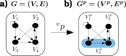
Figure 2: Graph Partitioning. Illustration of a supergraph, ‘naturally’ induced by a partition of the node set. (a) The graph $G=(V,E)$, comprised of $n=4$ nodes $V=\{V_{1},V_{2},V_{3},V_{4}\}$ and $m=7$ edges $E=\{E_{11},E_{13},E_{14},E_{23},E_{24},E_{34},E_{42}\}$. (b) The supergraph $G^{p}=(V^{p},E^{p})$, obtained by grouping the nodes $V_{3}$ and $V_{4}$ into the supernode $V^{p}_{3}=\{V_{3},V_{4}\}$. It is comprised of $n^{p}=3$ nodes $V^{p}=\{V^{p}_{1},V^{p}_{2},V^{p}_{3}\}$, and $m^{p}=5$ edges $E^{p}$, given by: $E^{p}_{11}=\{E_{11}\},E^{p}_{13}=\{E_{13},E_{14}\},E^{p}_{23}=\{E_{23},E_{24}\},E^{p}_{32}=\{E_{42}\},\text{ and }E^{p}_{33}=\{E_{34}\}$.

III.4 The Partition Lattices of a Graph

In this section, we explain some general mathematical properties that arise when partitioning a graph. This provides for a deeper understanding of this framework, and sets the stage for the next sections.

Before we go into details of graph-specific partitioning, we point out some relevant properties of what in mathematics is known as partition lattices Birkhoff (1940). Assume we are given a finite, non-empty $n$-element set $X$. The total number of distinct partitions we can create of it is given by the Bell number $B(n)$ Bell (1938); Becker and Riordan (1948). The set of all possible partitions, which we denote by $P=\{P_{i}\;\vline\;i\in\{1,2,...,B(n)\}\}$, is a partially ordered set, since some of the elements of $P$ have a pair-wise relation, which is called the finer-than relation. A partition $P_{i}$ is said to be a refinement of a partition $P_{j}$, if every element of $P_{i}$ is a subset of some element of $P_{j}$. If this condition is fulfilled, one says that $P_{i}$ is finer than $P_{j}$, $P_{i}\leq P_{j}$, and vice versa, $P_{j}$ is coarser than $P_{i}$, $P_{j}\geq P_{i}$. Since $X$ is finite, every partition $P_{i}$ is bounded from below and from above with respect to this finer-than relation,

$$P_{f}\leq P_{i}\leq P_{c},\text{ for all }i\in\{1,2,...,B(n)\},$$ (22)

where $P_{f}$ is called the finest element of P, given by $P_{f}=\{\{X_{1}\},\{X_{2}\},...,\{X_{n}\}\}$, and $P_{c}$ is the coarsest element, given by the trivial partition $P_{c}=\{X\}$. This implies that each set of elements of $P$ has a finest upper bound and a coarsest lower bound. Therefore, the set of all possible partitions $P$ is called a partition lattice (or more precisely, a geometric lattice, since $X$ is finite Welsh (2010)). Any totally ordered subset of $P$ is called a chain, and any subset of $P$ for which there exists no relation between any two different elements of that subset is called an antichain.

Since in this paper we are dealing with finite graphs exclusively, we can directly build the lattices of the node set $V$ and the edge set $E$, and translate the above properties of lattices into the context of graphs. However, we will also make use of the natural way of partitioning a graph as demonstrated in Sec. III.3, in order to create the geometric lattice of a graph $G=(V,E)$. This lattice, by construction, entails the lattice of the node set $V$, and a specific subset of the lattice of the edge set $E$, and there are therefore two lattices of interest: the lattice of a graph $G$, and the lattice of its edges $E$.

Let us note down the lattice of a graph $G$ with $n$ nodes and $m$ edges, for which there is a total of $B(n)$ different supergraphs. We create the set of all distinct partitions of $V$ by prescribing a set of functions ${}^{v}p=\{{}^{v}p^{k}\;\vline\;k\in\{1,2,...,B(n)\}\}$, such that each function

$${}^{v}p^{k}:V\rightarrow{}^{v}S^{k}=\{1,2,...,n^{{}p^{k}}\},$$ (23)

$$V_{i}\mapsto{}^{v}p^{k}(V_{i}):={}^{v}S^{k}_{i}\in{}^{v}S^{k},k\in\{1,2,...,B(n)\},$$ (24)

induces a supergraph $G^{p^{k}}=(V^{p^{k}},E^{p^{k}})$ as demonstrated in Sec. III.3 and illustrated in Fig. 2. The partition lattice of $V$, induced by the set of functions ${}^{v}p$, is therefore given by ${}^{V}L=\{V^{p^{k}}\;\vline\;k\in\{1,2,...,B(n)\}\}$. The finer-than relation between partitions translated to the lattice of $V$ means that if $V^{p^{k}}\leq V^{p^{l}}$, then every supernode $V^{p^{l}}_{i}$ of $V^{p^{l}}$ is the union of supernodes $V^{p^{k}}_{j}\in V^{p^{k}}$. We transfer the finer-than relation to graphs, by saying that $G^{p^{k}}\leq G^{p^{l}}$, if both $V^{p^{k}}\leq V^{p^{l}}$ and $E^{p^{k}}\leq E^{p^{l}}$. With reference to Eqs. (19)-(21), we see that for all partitions $V^{p^{k}}\leq V^{p^{l}}$, it follows that $E^{p^{k}}\leq E^{p^{l}}$ by construction, and consequently, we denote with ${}^{G}L=\{G^{p^{k}}\;\vline\;k\in\{1,2,...,B(n)\}$ the partition lattice of $G$, henceforth referred to as the deep graph of $G$. The lattice of the graph depicted in Fig. 2(a) is illustrated in Fig. 3(a). Some of its properties are: the finest element of ${}^{G}L$ is the graph $G=(V,E)$ itself; the coarsest element, which we denote by $G^{p^{c}}=(V^{p^{c}},E^{p^{c}})$, consists of one supernode connected to itself by a single superedge; and every chain in ${}^{G}L$, illustrated by the red, dashed lines in Fig. 3(a), corresponds to some agglomerative, hierarchical clustering of the nodes of $G$. The dashed blue lines in Fig. 3(b) will be explained in the next section.

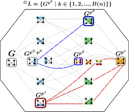
Figure 3: A deep graph, i.e. the geometric partition lattice of a graph. (a) Illustration of the graph $G=(V,E)$ as described in Fig. 2(a) (on the very left of the plot), and its $B(n)=15$ corresponding supergraphs, ordered by refinement from the right to the left. The supergraph $G^{p^{1}}$ is illustrated in detail in Fig. 2(b). Each link in this Hasse diagram corresponds to the finer-than relation between a pair of supergraphs. The dashed lines colored in red correspond to chains in the lattice. (b) An intersection partition is illustrated by $G^{p^{2}\cdot p^{3}}$, which results from intersecting $G^{p^{2}}$ and $G^{p^{3}}$. It constitutes a refinement of both $G^{p^{2}}$ and $G^{p^{3}}$ (blue dashed lines). The figure is a modification of Commons (2015).

However, the lattice of $E$ is generally not covered entirely by the lattice of $G$. In fact, maximally $B(n)$ of $B(m)$ possible partitions of $E$ are contained in ${}^{G}L$, due to the partitioning of $E$ by correspondence [see Eqs. (19)-(21)]. The full lattice of $E$ can be created analogously to that of $V$, by prescribing a set of functions ${}^{e}p=\{{}^{e}p^{k}\;\vline\;k\in\{1,2,...,B(m)\}\}$, such that each function

$${}^{e}p^{k}:E\rightarrow{}^{e}S^{k}=\{1,2,...,m^{p^{k}}\},$$ (25)

$$E_{ij}\mapsto{}^{e}p^{k}(E_{ij}):={}^{e}S^{k}_{r}\in{}^{e}S^{k},k\in\{1,2,...,B(m)\},$$ (26)

induces a partition $E^{p^{k}}$ of $E$ as demonstrated in Eqs. (14)-(17). The lattice of $E$ is then given by ${}^{E}L=\{E^{p^{k}}\;\vline\;k\in\{1,2,...,B(m)\}\}$.

In the next section, we introduce a useful tool that can be used to navigate the lattices ${}^{G}L$ and ${}^{E}L$ for the sake of creating meaningful partitions, based on the features and relations of a given graph.

III.5 Intersection Partitions

Due to the rapid increase of possible partitions with growing numbers of nodes and edges, it is only possible to actually compute the full lattices of $G$ and $E$ for very small graphs. However, we are generally not interested in every single partition, but rather a meaningful subset of them. Here, we demonstrate how to create intersection partitions and thereby establish a valuable tool to find potentially informative partitions, based on the features and relations of a graph. Furthermore, as we will demonstrate later on, one can utilize intersection partitions in order to compute similarity measures between different partitions. We will also make use of intersection partitions in Sec. IV.2 in order to derive a tensor-like representation of a multilayer network De Domenico et al. (2013).

To begin with, let us demonstrate what we mean by intersection partitions with a simple example. Imagine a standard $52$-card deck, partitioned by color on the one hand (red and black, both comprised of $26$ cards), and by suit on the other hand (spades, diamonds, hearts and clubs, each comprised of $13$ cards). The intersection partition of color and suit would then be comprised of $8$ elements: cards that are red and at the same time spades ($0$ cards); red & diamonds ($13$ cards); etc. Before showing some examples with regard to the exemplary graph in Fig. 1, let us note down the different ways of creating intersection partitions of a graph.

We first demonstrate the construction of intersection partitions of $V$. Assume we are given a set of $K$ [$\leq B(n)$] partitions of $V$, induced by a set of functions ${}^{v}p=\{{}^{v}p^{k}\;\vline\;k\in I^{K}\}$, where $I^{K}=\{1,2,...,K\}$ is the partition index set. From this set of available partitions, we choose a collection $g\subseteq I^{K}$, which is used to create an intersection partition. We define an element $V^{\underline{p}}_{\underline{i}}$ of the intersection partition $V^{\underline{p}}$ by

$$V^{\underline{p}}_{\underline{i}}:=\{V_{j}\;\vline\;j\in\{1,2,...,n\}\land\forall k\in g:{}^{v}p^{k}(V_{j})={}^{v}S^{k}_{i^{k}}\},\text{ where}$$ (27)

$$\underline{p}=(p^{k})_{k\in g},\underline{i}=(i^{k})_{k\in g},i^{k}\in\{1,2,...,n^{p^{k}}\},$$ (28)

and the intersection partition itself by

$$V^{\underline{p}}:=\bigcup_{\underline{i}}V^{\underline{p}}_{\underline{i}}.$$ (29)

Since $\varnothing\notin V^{\underline{p}}$ by construction, and by showing that

$$V^{\underline{p}}_{\underline{i}}\cap V^{\underline{p}}_{\underline{j}}=\varnothing\text{ for all }V^{\underline{p}}_{\underline{i}}\neq V^{\underline{p}}_{\underline{j}}\in V^{\underline{p}},\text{ where}$$ (30)

$$\underline{j}=(j^{k})_{k\in g},j^{k}\in\{1,2,...,n^{p^{k}}\},$$ (31)

we see that $V^{\underline{p}}$ is indeed a partition of $V$. A supernode $V^{\underline{p}}_{\underline{i}}$ of an intersection partition is comprised of $n^{\underline{p},\underline{i}}:=|V^{\underline{p}}_{\underline{i}}|$ nodes $V_{j}$ of $G$ that simultaneously belong to all supernodes ${}^{v}S^{k}_{i^{k}}$ chosen by $g$. The number of supernodes of an intersection partition, $n^{\underline{p}}:=|V^{\underline{p}}|$, is bounded by $\prod_{k\in g}n^{p^{k}}$, and every intersection partition constitutes a refinement of the partitions it has been constructed from, $V^{\underline{p}}\leq V^{p^{k}}$ for all $k\in g$. The number of distinct intersection partitions we can construct from $I^{K}$ is bounded from above by $I(K)=\sum_{|g|=0}^{K}\binom{K}{|g|}=|\mathcal{P}(I^{K})|$, where $\mathcal{P}(I^{K})$ is the power set of the partition index set, hence $I(K)=2^{K}$. Looking at Fig. 1, the intersection partition of the collection of partitions $g=\{\text{`category'},\text{`political ideology'}\}$ would yield $n^{\underline{p}}=10$ supernodes. The supernodes comprised of more than $1$ node of $G$ would be: ‘person’ & ‘egalitarianism’ (3 nodes); ‘person’ & ‘environmentalism’ (2 nodes); and ‘state’ & ‘conservatism’ (2 nodes).

Defining the corresponding intersection partition $E^{\underline{p}}$ of $E$ into $m^{\underline{p}}:=|E^{\underline{p}}|$ superedges $E^{\underline{p}}_{\underline{i}\underline{j}}$ by

$$E^{\underline{p}}_{\underline{i}\underline{j}}:=\{E_{uv}\;\vline\;\Phi^{e}(u,v)\wedge\forall k\in g:{}^{v}p^{k}(V_{u})={}^{v}S^{k}_{i^{k}}\wedge\forall k\in g:{}^{v}p^{k}(V_{v})={}^{v}S^{k}_{j^{k}}\}$$ (32)

and $E^{\underline{p}}:=\bigcup_{\underline{i},\underline{j}}E^{\underline{p}}_{\underline{i}\underline{j}}$, it follows that $\underline{p}$ induces a supergraph $G^{\underline{p}}=(V^{\underline{p}},E^{\underline{p}})$, in analogy to Eqs. (19)-(21). A superedge $E^{\underline{p}}_{\underline{i}\underline{j}}$ is comprised of $m^{\underline{p},\underline{i}\underline{j}}:=|E^{\underline{p}}_{\underline{i}\underline{j}}|$ edges $E_{uv}$ originating from nodes in supernode $V^{\underline{p}}_{\underline{i}}$ and targeting nodes in supernode $V^{\underline{p}}_{\underline{j}}$. Figure 3(b) depicts a supergraph, created from intersecting two different supergraphs.

With regard to partitioning the edges of a graph, however, there are other options than partitioning by types of relations [see Eqs. (14)-(17)], or by correspondence [see Eqs. (19)-(21)]. We now show how to utilize the edges’ relations and the features of their incident nodes in all possible combinations. For instance, regarding the graph in Fig. 1, we might want to know how many edges originate from nodes with a ‘political ideology’ of ‘egalitarianism’, or ‘conservatism’, etc. The answer would yield a total of $m^{p}=5$ superedges, originating from: ‘anarchism’ (comprised of 9 edges); ‘egalitarianism’ (5 edges); ‘conservatism’ (2 edges); ‘environmentalism’ (5 edges); and ‘neoliberalism’ (1 edge). These superedges, however, could be refined by asking how many of their constituent edges target nodes of the ‘category’ ‘bank’, or ‘company’ and so forth. We would then see, for instance, that the edges originating from nodes with a ‘political ideology’ of ‘egalitarianism’ all target nodes of the ‘category’ ‘state’. Refining these superedges even further, we could ask, how many edges originating from nodes with a ‘political ideology’ of ‘egalitarianism’ and targeting nodes of the ‘category’ ‘state’ are of the ‘kind of payment’ ‘tax’, or ‘bribe’, etc. Let us note down all the combinations formally, to clarify the procedure of partitioning edges.

Assume we are given a set of ${}^{v}K$ partitions of $V$, induced by ${}^{v}p=\{{}^{v}p^{k}\;\vline\;k\in{}^{v}I^{K}\}$, where ${}^{v}I^{K}=\{1,2,...,{}^{v}K\}$ is the partition index set of the nodes. Additionally, we have a set of ${}^{e}K$ partitions of $E$, induced by ${}^{e}p=\{{}^{e}p^{k}\;\vline\;k\in{}^{e}I^{K}\}$, where ${}^{e}I^{K}=\{1,2,...,{}^{e}K\}$ is the partition index set of the edges. From these partitions, we choose three different collections: a source type collection $g^{s}\subseteq{}^{v}I^{K}$, a target type collection $g^{t}\subseteq{}^{v}I^{K}$ and a relation type collection $g^{r}\subseteq{}^{e}I^{K}$. Then, we denote a superedge by $E^{\underline{p}}_{\underline{i}\underline{j},\underline{r}}$, where

$$\underline{p}=\left(({}^{s}p^{k})_{k\in g^{s}},({}^{t}p^{k})_{k\in g^{t}},({}^{r}p^{k})_{k\in g^{r}})\right),$$ (33)

$$\underline{i}=(i^{k})_{k\in g^{s}},\text{ with }i^{k}\in\{1,2,...,n^{p^{k}}\},$$ (34)

$$\underline{j}=(j^{k})_{k\in g^{t}},\text{ with }j^{k}\in\{1,2,...,n^{p^{k}}\},\text{ and}$$ (35)

$$\underline{r}=(r^{k})_{k\in g^{r}},\text{ with }r^{k}\in\{1,2,...,m^{p^{k}}\},$$ (36)

and define it by

$$E^{\underline{p}}_{\underline{i}\underline{j},\underline{r}}:=\{E_{uv}\;\vline\;\Phi^{e}(u,v)\land\Phi^{v}_{g^{s}}(u)\land\Phi^{v}_{g^{t}}(v)\land\Phi^{e}_{g^{r}}(u,v)\},\text{ where}$$ (37)

$$\Phi^{v}_{g^{s}}(u):(\forall k\in g^{s}:{}^{v}p^{k}(V_{u})={}^{v}S^{k}_{i^{k}}),$$ (38)

$$\Phi^{v}_{g^{t}}(v):(\forall k\in g^{t}:{}^{v}p^{k}(V_{v})={}^{v}S^{k}_{j^{k}}),\text{ and}$$ (39)

$$\Phi^{e}_{g^{r}}(u,v):(\forall k\in g^{r}:{}^{e}p^{k}(E_{uv})={}^{e}S^{k}_{r^{k}}).$$ (40)

The partition $E^{\underline{p}}$ of $E$ is then given by $E^{\underline{p}}:=\bigcup_{\underline{i},\underline{j},\underline{r}}E^{\underline{p}}_{\underline{i}\underline{j},\underline{r}}$. Based on these definitions, we denote the number of superedges by $m^{\underline{p}}=|E^{\underline{p}}|$, and the number of edges contained in a superedge by $m^{\underline{p},\underline{i}\underline{j},\underline{r}}:=|E^{\underline{p}}_{\underline{i}\underline{j},\underline{r}}|$. If all collections are empty at the same time, $g^{x}=\varnothing$ for all $x\in\{s,t,r\}$, it follows that $E^{\underline{p}}_{\underline{i}\underline{j},\underline{r}}=E$, which means that the edge set is partitioned into the trivial partition, comprised of one superedge entailing all edges. Furthermore, if we choose $g^{s}=g^{t}$ and $g^{r}=\varnothing$, we get the definition of the corresponding partition, as stated in Eq. (32). Expressed formally, the example stated in the above paragraph would hence be described as follows: we choose the source type collection by $g^{s}=\{\text{`political ideology'}\}$, the target type collection by $g^{t}=\{\text{`category'}\}$ and the relation type collection by $g^{r}=\{\text{`kind of payment'}\}$. The superedge $E^{\underline{p}}_{\underline{i}\underline{j},\underline{r}}$ corresponding to $\underline{i}=(\text{`egalitarianism'})$, $\underline{j}=(\text{`state'})$ and $\underline{r}=(\text{`tax'})$ would then be comprised of $m^{\underline{p},\underline{i}\underline{j},\underline{r}}=5$ edges.

Before we turn to the next section, let us make some general remarks regarding intersection partitions:

i) First of all, it is noteworthy that it only makes sense to create intersection partitions of antichains, since any chain in $g$, $g^{s}$, $g^{t}$ or $g^{r}$ can be replaced by the finest element of the respective chain.

ii) When creating intersection partitions we have to be aware of the fact that a supernode $V^{\underline{p}}_{\underline{i}}$ might be comprised of zero nodes, $n^{\underline{p},\underline{i}}=0$. In this case, we say the supernode $V^{\underline{p}}_{\underline{i}}$ does not exist. This stands in contrast to the supernodes $V^{p^{k}}_{i}$ of supergraphs $G^{p^{k}}$, for which $n^{p,i}\geq 1$ for all $i\in\{1,2,...,n^{p^{k}}\}$, since we chose the functions ${}^{v}p^{k}$ to be surjective. This does not pose a problem though, since for a superedge $E^{\underline{p}}_{\underline{i}\underline{j}}$ with $m^{\underline{p},\underline{i}\underline{j}}=0$, we can still deduce if the superedge does not exist because at least one of the supernodes does not exist ($n^{\underline{p},\underline{i}}$ or $n^{\underline{p},\underline{j}}=0$), or because there is in fact no superedge between existing supernodes ($n^{\underline{p},\underline{i}}$ and $n^{\underline{p},\underline{j}}\geq 1$).

iii) Finally, we want to refer to Appendix A, where we demonstrate how to utilize intersection partitions in order to compute similarity measures between different (intersection) partitions. Such measures can be utilized, for instance, to assess the community structure of time-evolving networks, as the authors of Granell et al. (2015) have demonstrated.

III.6 Redistribution and Allocation of Information on the Lattices

The last sections were dedicated to constructing partitions, allowing us to group any desirable subset of nodes and edges into supernodes and superedges, respectively. Here, we demonstrate that the information of a graph – expressed by the features and relations of its constituent nodes and edges – is not only conserved under partitioning, but redistributed on the partition lattices, according to the partition function(s) we choose. This allows us to aggregate data of any desirable group of nodes or edges. We then demonstrate how to allocate partition-specific features and relations, which also allows us to create superedges independently of the edges in $G$.

First, the information contained in a given graph $G=(V,E)$ is conserved when creating partitions: given a partition $V^{\underline{p}}$ of $V$ induced by $\underline{p}$ [see Eqs. (27)-(29)], every supernode $V^{\underline{p}}_{\underline{i}}\in V^{\underline{p}}$ is a subset of the nodes of $G$, where each node is comprised of a set of features. The complete set of features contained in supernode $V^{\underline{p}}_{\underline{i}}$ can then be partitioned by their corresponding types, and therefore expressed as a collection of sets of features of common type. Hence, a supernode $V^{\underline{p}}_{\underline{i}}$ – expressed in terms of its constituent features – is given by

$$V^{\underline{p}}_{\underline{i}}=\{\underline{i}\}\cup\{F^{\underline{p},T}_{\underline{i},t}\}_{t\in\{1,2,...,n^{\underline{p},\underline{i}}_{\text{types}}\}},$$ (41)

where the number of distinct types of features in supernode $V^{\underline{p}}_{\underline{i}}$ is denoted by $n^{\underline{p},\underline{i}}_{\text{types}}$, and the number of features of type $t$ by $n^{\underline{p},\underline{i}}_{\text{t}}:=|F^{\underline{p},T}_{\underline{i},t}|$. Looking at Fig. 1, the supernode comprised of the nodes with indices $(2,6,11)$, for instance, has a total of $n^{\underline{p},\underline{i}}_{\text{types}}=7$ types of features: ‘category’ ($n^{\underline{p},\underline{i}}_{1}=3$: ‘person’: 2 nodes, ‘company’: 1 node); ‘name’ ($n^{\underline{p},\underline{i}}_{2}=3$: ‘Avon Barksdale’: 1 node, ‘Rust Cohle’: 1 node, ‘Viktor’s Gun Shop’: 1 node); ‘occupation’ ($n^{\underline{p},\underline{i}}_{3}=2$: ‘chief executive officer’: 1 node, ‘federal police officer’: 1 node); ‘age’ ($n^{\underline{p},\underline{i}}_{4}=3$: ‘91’: 1 node, ‘61’: 1 node, ‘141’: 1 node); etc. By this example, it becomes clear that we can easily create frequency distributions of the values of a supernodes’ different types of features.

Analogously, we can express superedges in terms of the relations of their constituent edges’, which we also partition by their corresponding types: given a partition $E^{\underline{p}}$ of $E$ induced by $\underline{p}$ [see Eqs. (33)-(40)], a superedge $E^{\underline{p}}_{\underline{i}\underline{j},\underline{r}}$ is given by

$$E^{\underline{p}}_{\underline{i}\underline{j},\underline{r}}=\{(\underline{i},\underline{j},\underline{r})\}\cup\{R^{\underline{p},T}_{\underline{i}\underline{j},\underline{r},t}\}_{t\in\{1,2,...,m^{\underline{p},\underline{i}\underline{j},\underline{r}}_{\text{types}}\}},$$ (42)

where the number of distinct types of relations in superedge $E^{\underline{p}}_{\underline{i}\underline{j},\underline{r}}$ is denoted by $m^{\underline{p},\underline{i}\underline{j},\underline{r}}_{\text{types}}$, and the number of relations of type $t$ by $m^{\underline{p},\underline{i}\underline{j},\underline{r}}_{\text{t}}:=|R^{\underline{p},T}_{\underline{i}\underline{j},\underline{r},t}|$. For mathematical details, we refer to Appendix B.

By this representation of supernodes and superedges, we can clearly see that the information of a graph $G$ is not only conserved under partitioning, but redistributed according to the partition function(s) we choose. This means that every supergraph $G^{\underline{p}}$ on the lattice ${}^{G}L$, and every partition $E^{\underline{p}}$ on the lattice ${}^{E}L$, corresponds to a unique redistribution of the information contained in a graph $G$, and the collection of all possible redistributions is given by the lattices ${}^{G}L$ and ${}^{E}L$.

Second, we show how to allocate partition-specific information on the lattice ${}^{G}L$. Note that we omit the vector notation of intersection partitions for the remainder of this section for reasons of notational simplicity. Given a supergraph $G^{p}\in{}^{G}L$, we know that its supernodes are comprised of features $\{F^{p,T}_{i,t}\}_{t\in\{1,2,...,n^{p,i}_{\text{types}}\}}$, and its superedges are comprised of relations $\{R^{p,T}_{ij,t}\}_{t\in\{1,2,...,m^{p,ij}_{\text{types}}\}}$. Based on these features and relations, we can compute additional properties (e.g., moments, correlations) by applying some set of functions on them. For the sake of notational convenience, we write single functions mapping to sets of new properties:

$$f(\{F^{p,T}_{i,t}\}_{t\in\{1,2,...,n^{p,i}_{\text{types}}\}})=\{{}^{p}F^{p,T}_{i,t}\}_{t\in\{1,2,...,{}^{p}n^{p,i}_{\text{types}}\}},$$ (43)

$$f(\{R^{p,T}_{ij,t}\}_{t\in\{1,2,...,m^{p,ij}_{\text{types}}\}})=\{{}^{p}R^{p,T}_{ij,t}\}_{t\in\{1,2,...,{}^{p}m^{p,ij}_{\text{types}}\}},$$ (44)

where the additional $p$-index on the upper left corner indicates that these features and relations are specific to the supergraph $G^{p}$. Of course, we can also allocate features to supernodes independently from the features of the supernodes’ constituent nodes. The same goes for the relations of superedges, even in the case when they are comprised of zero edges (for which $E^{p}_{ij}=\varnothing$ and therefore also $\{R^{p,T}_{ij,t}\}_{t\in\{1,2,...,m^{p,ij}_{\text{types}}\}}=\varnothing$). We do not, however, denote these independently allocated features and relations differently to the computed features and relations in Eqs. (43) and (44). Hence, the properties of supernodes and superedges of a supergraph can be written as

$$V^{p}_{i}=\{i\}\cup\{F^{p,T}_{i,t}\}_{t\in\{1,2,...,n^{p,i}_{\text{types}}\}}\cup\{{}^{p}F^{p,T}_{i,t}\}_{t\in\{1,2,...,{}^{p}n^{p,i}_{\text{types}}\}},$$ (45)

and

$$E^{p}_{ij}=\{(i,j)\}\cup\{R^{p,T}_{ij,t}\}_{t\in\{1,2,...,m^{p,ij}_{\text{types}}\}}\cup\{{}^{p}R^{p,T}_{ij,t}\}_{t\in\{1,2,...,{}^{p}m^{p,ij}_{\text{types}}\}}.$$ (46)

Of course, the partition-specific features and relations only bear meaning for the unique element of the lattice $G^{p}\in{}^{G}L$. Furthermore, they can only be redistributed on the set of all coarser supergraphs, given by the chains entailed in $\{G^{p^{\prime}}\;\vline\;p^{\prime}\in\{1,2,...,B(n)\}\land p^{\prime}>p\}\subseteq{}^{G}L$ (see the red, dashed lines in Fig. 3).

IV Deep Graph Construction

The theoretical framework satisfying the objectives stated in the Introduction is now fully described. Here, we want to roughly describe the general procedure of constructing a deep graph. For this purpose, we introduce two types of auxiliary functions: connectors, which are functions allowing us to create (super)edges between (super)nodes, purely based on the properties of the represented objects; and selectors, which are functions allowing us to select (i.e. filter) (super)edges, based on their respective properties. In combination, these functions effectively allow us to forge the topology of a deep graph, which we will exemplify in Sec. V. Furthermore, we demonstrate in this section how our framework integrates with existing network theory and other data analysis tools, and finally make some general remarks regarding the identification of (super)nodes, (super)edges and partitions.

IV.1 Outline of Deep Graph Construction

Given a set of $n$ objects, the general procedure of constructing a deep graph can be outlined as follows

1. identify each object as a node $V_{i}$, $i=1,2,...,n$.

2. assign features to each node $V_{i}$, $V_{i}=\{i,F_{i}^{1},F_{i}^{1},...,F_{i}^{f_{i}}\}$.

3. define connectors

   $$m_{ij}(V_{i},V_{j}):=E_{ij}=\{(i,j),R^{1}_{ij},R^{2}_{ij},...,R^{r_{ij}}_{ij}\},$$ (47)

   where $m_{ij}$ is a function mapping a pair of sets of features to a set of relations. Connector functions create “computable”, or “external” relations between objects. They are typically based on distance or similarity measures of objects, or some information or physical flow between them. A few examples are the scalar product of vectors, the distance of objects in a metric space, or correlation coefficients between variables. Networks solely based on one such measure are often termed functional networks Boers et al. (2013); Zhou et al. (2006).

4. create the set of all possible edges $E^{\prime}$ by applying the connector functions on all pairs of nodes.

5. if there is any a priori knowledge of relations between the objects (as opposed to the computed relations by connectors), append them to the corresponding edges. By a priori known relations, we mean any inherent, internal, physical, trivial or abstract relations, such as flightpaths between airports, synapses between neurons, social relationships between humans, or relations of plants to the treatment of medical conditions.

6. define selectors

   $$s_{ij}(E_{ij}):=\begin{cases}E_{ij}&\text{if }E_{ij}\text{ satisfies conditions of }s_{ij}\\ \varnothing&\text{if }E_{ij}\text{ does not satisfy conditions of }s_{ij}\end{cases},$$ (48)

   where $s_{ij}$ is a function mapping a set of relations to itself, if the set satisfies the conditions expressed in the function, or to an empty set otherwise, thereby removing the corresponding edge from the edge set $E$. Selectors can be simple thresholding functions (e.g., for some features $F^{k}_{j}$ and $F^{l}_{i}$: $E_{ij}\mapsto E_{ij}$ if $(F^{k}_{j}-F^{l}_{i})\leq T$, else $E_{ij}\mapsto\varnothing$), but they can also be more complicated and elaborate, involving different types of relations at the same time.

7. select $E\subseteq E^{\prime}$ by applying the selector functions on all edges $E^{\prime}$.

The graph is then given by $G=(V,E)$, where the objects’ properties are represented by sets of features $V_{i}$, and the relational information of pairs of objects is represented by sets of relations $E_{ij}$.

The next step is to repeat the following procedure for any supergraph $G^{p}\in{}^{G}L$ for which we want to allocate, aggregate or evaluate information. Again, for notational clarity, we omit vector notation.

1. identify a partition $G^{p}$ of $G$. This partition might be induced by the (intersection of) features of the nodes in $G$ (see Sec. III.1 and Sec. III.5), or created by any other means, such as manual assignment of supernode labels, clustering algorithms, community detection algorithms, or partitioning by the connected components of $G$.

2. compute and allocate partition-specific features to any of the supernodes

   $$V^{p}_{i}=\{i\}\cup\{F^{p,T}_{i,t}\}_{t\in\{1,2,...,n^{p,i}_{\text{types}}\}}\cup\{{}^{p}F^{p,T}_{i,t}\}_{t\in\{1,2,...,{}^{p}n^{p,i}_{\text{types}}\}}.$$

3. compute and allocate partition-specific relations to any of the superedges

   $$E^{p}_{ij}=\{(i,j)\}\cup\{R^{p,T}_{ij,t}\}_{t\in\{1,2,...,m^{p,ij}_{\text{types}}\}}\cup\{{}^{p}R^{p,T}_{ij,t}\}_{t\in\{1,2,...,{}^{p}m^{p,ij}_{\text{types}}\}}.$$

4. define connectors between supernodes,

   $$m_{ij}:V^{p}\times V^{p}\rightarrow E^{\prime p},(V^{p}_{i},V^{p}_{j})\mapsto m_{ij}(V^{p}_{i},V^{p}_{j}),$$

   to further enrich the relations of the superedges in $G^{p}$,

   $$E^{p}_{ij}=\{(i,j)\}\cup\{R^{p,T}_{ij,t}\}_{t\in\{1,2,...,m^{p,ij}_{\text{types}}\}}\cup\{{}^{p}R^{p,T}_{ij,t}\}_{t\in\{1,2,...,{}^{p}m^{p,ij}_{\text{types}}\}}\cup m_{ij}(V^{p}_{i},V^{p}_{j}).$$

5. define selectors on the set of superedges,

   $$s_{ij}(E^{p}_{ij}):=\begin{cases}E^{p}_{ij}&\text{if }E^{p}_{ij}\text{ satisfies conditions of }s_{ij}\\ \varnothing&\text{if }E^{p}_{ij}\text{ does not satisfy conditions of }s_{ij}\end{cases}.$$

6. select $E^{p}\subseteq E^{\prime p}$ by applying the selector functions on all edges $E^{\prime p}$.

The supergraph is then represented by $G^{p}=(V^{p},E^{p})$. Repeating this procedure for different elements $G^{p}\in{}^{G}L$, we continuously extend the information contained in ${}^{G}L$. This information, in turn, can then be redistributed on the lattice (see Sec. III.6, and the red lines in Fig. 3), and increases the number of possible ways to create intersection partitions (see Sec. III.5, and the blue lines in Fig. 3).

IV.2 Imposing Traditional Graph Representations

Here, we show how to obtain existing network representations, by imposing certain restrictions on our framework resulting in the multilayer network (MLN) representation, as defined by Kivelä et al Kivelä et al. (2014). We chose to demonstrate only the attainment of the MLN representation for two reasons. First, because it is – to the best of our knowledge – the most general framework of network representation today, and second, because it allows us refer to the extensive work done by Kivelä et al Kivelä et al. (2014), Boccaletti et al Boccaletti et al. (2014), and references therein. In these papers, the reader can find derivations of many additionally constrained network representations down to the level of ordinary graphs Bollobas (1998), as well as a compendium of network tools, models and concepts to analyze networks. Therefore, the derivation of the MLN representation – in conjunction with the work done in these papers – allows us to exploit the already existing tool set of network theory.

For readers unfamiliar with MLNs, we provide a summary in Appendix A. Without loss of generality, we assume a MLN $M=(V_{M},E_{M},V^{N},\bm{L})$ with $|V^{N}|=:N$ nodes and $|V_{M}|=:n\leq|V^{N}|\cdot\prod^{d}_{a=1}|L_{a}|$ node-layers. First, we have to restrict ourselves to the representation of a single element of the partition lattice of a deep graph, $G^{p}\in{}^{G}L$. Let us assume that this element is the finest element of ${}^{G}L$ w.l.o.g., $G=(V,E)$. Then, there are two choices of $G$, resulting in distinct representations of $M$. We can place the additional information attributed to the layered structure of $M$ either in the nodes of $G$, or in the edges of $G$. The latter case is described in Appendix D. The former case, which is the favourable representation of $M$, is described in the following.

We identify each node $V_{i}\in V=\{V_{1},V_{2},...,V_{n}\}$ with a node-layer $V_{M,i}\in V_{M}$, such that

$$V_{i}=\{V^{N}_{i},L_{1,i},L_{2,i},...,L_{d,i}\}\mathrel{\widehat{=}}V_{M,i}\in V^{N}\times L_{1}\times L_{2}\times\cdot\cdot\cdot\times L_{d},$$ (49)

where $V^{N}_{i}\in V^{N}$ and $L_{a,i}\in L_{a}$ for all $a\in\{1,2,...,d\}$. This means that every node $V_{i}$ of $G$ has one feature corresponding to the index of a node $V^{N}_{i}\in V^{N}$ and $d$ features corresponding to elementary layers of the aspects $L_{a}\in\bm{L}$. An edge $E_{ij}\in E^{\prime}=\{E_{11},E_{12},...,E_{nn}\}$ is given by

$$E_{ij}=\begin{cases}\{w\left((V_{M,i},V_{M,j})\right)\}&\text{if }(V_{M,i},V_{M,j})\in E_{M}\\ \varnothing&\text{if }(V_{M,i},V_{M,j})\notin E_{M}\end{cases}.$$ (50)

Therefore, the edge set $E$ corresponding to $E_{M}$ is given by $E=\{E_{ij}\;\vline\;i,j\in\{1,2,...,n\}\land E_{ij}\neq\varnothing\}$. Every edge $E_{ij}\in E$ has exactly one relation, whose type is determined by the tuple of features $(\{L_{a,i}\}^{d}_{a=1},\{L_{a,j}\}^{d}_{a=1})$ of the adjacent nodes $V_{i}$ and $V_{j}$. The derived representation $G=(V,E)$ corresponds one to one to the ‘supra-graph’ representation of a MLN, given by the tuple $(V_{M},E_{M})$. Figure 4 shows an examplary MLN, side by side with its representation derived here and a tensor-like representation we derive in Appendix D.

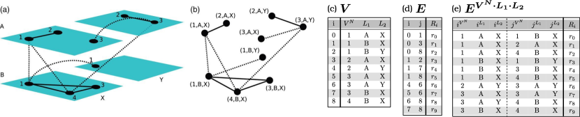
Figure 4: An exemplary multilayer network (MLN) and its representation by our framework. (a) An exemplary MLN, $M=(V_{M},E_{M},V^{N},\bm{L})$, consisting of four nodes, $V^{N}=\{1,2,3,4\}$, and two aspects, $\bm{L}=\{L_{1},L_{2}\}$, where $L_{1}=\{A,B\}$ and $L_{2}=\{X,Y\}$. It has a total of 9 node-layers, $V_{M}=\{(1,A,X),(1,B,X),(1,B,Y),(2,A,X),(2,A,Y),(3,A,X),(3,A,Y),(3,B,X),(4,B,X)\}$, connected pair-wise by a total of 10 edges, $E_{M}\subset V_{M}\times V_{M}$. For notational brevity, we consider the edges to be directed (with randomly chosen directions). (b) The same MLN as in (a), depicted by its underlying ‘supra-graph’ representation, $G_{M}=(V_{M},E_{M})$. (c) The nodes $V_{i}\in V$ of the graph $G=(V,E)$, representing the MLN described in (a). $G$ has a total of 9 nodes (corresponding to the MLN’s node-layers), whose indices are given by the left column. The top row indicates the nodes’ types of features, which correspond one-to-one to the MLN’s node indices and its aspects. (d) The edges $E_{ij}\in E$ of the graph $G=(V,E)$, representing the MLN described in (a). $G$ has a total of 10 edges, corresponding to the edges $E_{M}$ of $M$. The first two columns indicate the indices of edges $E_{ij}$ from node $V_{i}$ to node $V_{j}$. The (complex- or real-valued) relations of the edges are denoted by $r_{i}$ and their corresponding types by $R_{i}$ (which are condensed into one column, for reasons of space). (e) A tensor-like representation of the edges of the MLN described in (a). It is derived from the graph $G$ [see (c) and (d)], by constructing the intersection partition of all its types of features, resulting in the supergraph $G^{V^{N}\cdot L_{1}\cdot L_{2}}=(V^{V^{N}\cdot L_{1}\cdot L_{2}},E^{V^{N}\cdot L_{1}\cdot L_{2}})$. The supergraph’s edges $E^{V^{N}\cdot L_{1}\cdot L_{2}}_{i^{V^{N}}\cdot i^{L_{1}}\cdot i^{L_{2}},j^{V^{N}}\cdot j^{L_{1}}\cdot j^{L_{2}}}\in E^{V^{N}\cdot L_{1}\cdot L_{2}}$ are indexed like a tensor, as apparent from the table. See Appendix D for mathematical details. Figure 4(a) and (b) are reproduced with permission from Journal of Complex Networks 2, 203 - 271 (2014). Copyright 2013 Oxford University Press - Journals.

In Appendix D, we demonstrate how the subset of the partition lattice ${}^{G}L$ of $G\mathrel{\widehat{=}}M$ induced by the types of features of its constituent nodes corresponds to different representations of a MLN, including the above mentioned tensor-like representation De Domenico et al. (2013). There, we also discuss the constraints imposed on our framework in order to obtain the MLN representation, and how our representation solves the issues encountered in the representation of MLNs.

IV.3 Integration with other Data Analysis Tools

As demonstrated above, the (super)nodes and (super)edges of a (super)graph $G^{\underline{p}}\in{}^{G}L$ are nothing less than collections of sets of mathematical objects,

$$V^{\underline{p}}_{\underline{i}}=\{\underline{i}\}\cup\{F^{\underline{p},T}_{\underline{i},t}\}_{t\in\{1,2,...,n^{\underline{p},\underline{i}}_{\text{types}}\}}\cup\{{}^{\underline{p}}F^{\underline{p},T}_{\underline{i},t}\}_{t\in\{1,2,...,{}^{\underline{p}}n^{\underline{p},\underline{i}}_{\text{types}}\}},\text{ and}$$ (51)

$$E^{\underline{p}}_{\underline{i}\underline{j}}=\{(\underline{i},\underline{j})\}\cup\{R^{\underline{p},T}_{\underline{i}\underline{j},t}\}_{t\in\{1,2,...,m^{\underline{p},\underline{i}\underline{j}}_{\text{types}}\}}\cup\{{}^{\underline{p}}R^{\underline{p},T}_{\underline{i}\underline{j},t}\}_{t\in\{1,2,...,{}^{\underline{p}}m^{\underline{p},\underline{i}\underline{j}}_{\text{types}}\}}\cup m_{\underline{i}\underline{j}}(V^{\underline{p}}_{\underline{i}},V^{\underline{p}}_{\underline{j}}),$$ (52)

just like the superedges of the partitions $E^{\underline{p}}\in{}^{E}L$ [see Eq. (42)]

$$E^{\underline{p}}_{\underline{i}\underline{j},\underline{r}}=\{(\underline{i},\underline{j},\underline{r})\}\cup\{R^{\underline{p},T}_{\underline{i}\underline{j},\underline{r},t}\}_{t\in\{1,2,...,m^{\underline{p},\underline{i}\underline{j},\underline{r}}_{\text{types}}\}}.$$ (53)

Therefore, there is nothing hindering us from utilizing the tool sets developed in fields such as multivariate statistics, probability theory, supervised and unsupervised machine learning, and graph theory, in order to analyze the properties of (super)nodes and their relations. For instance, we can use machine learning algorithms to predict missing features of nodes, or to predict relations between objects. We can use statistical tools to compute properties such as moments, ranges, covariances and cross-entropies. We can also compute graph theoretical measures, such as centrality measures (e.g. eigenvector centralities, betweenness centralities, closeness centralities, degree centralities), participation coefficients, matching indices or local clustering coefficients. Furthermore, we can compute similarity or distance measures through connector functions, and then use appropriate clustering algorithms, such as stochastic block models Aicher et al. (2013); Peixoto (2012, 2013, 2014), in order to find informative partitions. All these properties and labels can then be reassigned to the features and relations of the (super)nodes and (super)edges.

IV.4 Identification of (Super)Nodes, (Super)Edges and Partitions

The framework we have laid down offers a good deal of flexibility in mapping systems onto networks. For that reason, we want to conclude this section by making a number of general remarks regarding the identification of (super)nodes, (super)edges, their respective properties and partitions.

i) First of all, recall that the nodes of a graph represent arbitrary objects. There are no restrictions of what constitutes an object, so a node might represent literally anything that comes to mind. On top of that, the features of a node themselves can be arbitrary objects. This means, however, that the features of a node might themselves be identified as nodes, and vice versa. With regard to the exemplary graph in Fig. 1, for instance, the nodes with indices $8$ and $9$ (each representing a ‘state’) might just as well have been identified as features (of type ‘lives in’) of the nodes representing persons (indices $0$-$6$). Yet, we identified them as nodes connected by edges (with the type of relation ‘lives in’) to the nodes $0$-$6$. There are, of course, no general rules of what to identify as features, and what as nodes. This choice depends mainly on the context.

ii) A similar situation arises when dealing with variables $X=\{x_{i}\;\vline\;i\in\{1,2,...,n\}\}$. Imagine, for instance, a set of variables, each representing a time-series of measurements (e.g. of the channels in an EEG measurement). Then, each variable can be identified as a node, whose feature is the variable itself. But we could also identify each single value assumed by the variables as a node, and include features indicating the variables (supernodes) each node belongs to. Similar to the identification of the node-layers (as opposed to the nodes) of a MLN as the nodes of a deep graph (see Appendix B), the latter choice is more flexible, and actually contains the former choice as supernodes. By identifying each value of a time-series as a node, for instance, we can create additional supernode labels corresponding to discretizations of either axis (time or values), such as a discretization into a certain number of quantiles. Such a concept has been used in Campanharo et al. (2011) to create a map from a time series to a network with an approximate inverse operation. Within our framework, a bijection between a variable $X$ and the nodes of a graph $G$ is trivially given by

$$m_{b}:X\leftrightarrow V,x_{i}\mapsto m_{b}(x_{i}):=V_{i}=\{i,x_{i}\},$$ (54)

$$m_{b}^{-1}(m_{b}[X])=X.$$ (55)

Similarly, we can map multidimensional objects (or observations, in machine learning parlance)

$$X=\{\underline{x}_{i}=(x^{j}_{i})_{j\in\{1,2,...,p\}}\in\mathbb{R}^{p}\;\vline\;i\in\{1,2,...,n\}\}$$ (56)

to the nodes of a graph $G=(V,E)$, by a function

$$m_{b}:X\leftrightarrow V,\underline{x}_{i}\mapsto m_{b}(\underline{x}_{i}):=V_{i}=\{i,\underline{x}_{i}\},$$ (57)

$$m_{b}^{-1}(m_{b}[X])=X.$$ (58)

This allows us, for instance, to create edges between objects containing the derivatives of each pair of variables, $m(V_{i},V_{j}):=E_{ij}=\{\frac{x^{k}_{j}-x^{k}_{i}}{x^{l}_{j}-x^{l}_{i}}\}_{k\neq l\in\{1,2,...,p\}}$.

iii) It is also straightforward to represent and analyze recurrence networks Marwan (2008) by deep graphs. Given a $p$-dimensional phase space and a (discretized) phase-space trajectory represented by a temporal sequence of $p$-dimensional vectors $\underline{x}_{i}\in X$ [see Eq. 56], we first map each point $\underline{x}_{i}$ of the trajectory to a node $V_{i}$ as described in Eq. 57. Then, we create edges between these nodes, based on some metric on the given phase space (e.g., the euclidian distance), $m(V_{i},V_{j}):=E_{ij}=\{\|\underline{x}_{j}-\underline{x}_{i}\|\}$. Finally, we define a selector $s(E_{ij})$, $s(E_{ij})\mapsto E_{ij}$ if $\|\underline{x}_{j}-\underline{x}_{i}\|<\varepsilon$, else $s(E_{ij})\mapsto\varnothing$, leaving only edges between nodes with a distance smaller than $\varepsilon$, indicating the recurrence of a state in phase space. The recurrence network is then given by $G=(V,E)$. This approach can be generalized to cross and joint recurrence networks Marwan and Kurths (2002), by mapping a collection of phase space trajectories to the nodes of a graph (where to each node an additional feature is prescribed, indicating the trajectory it belongs to), and defining connectors and selectors accordingly.

iv) As a general rule of thumb, any divisible or separable entity of a system to be mapped to a deep graph should be divided into separate nodes, and their membership to the corresponding entity indicated by supernode labels.

v) A convenient manner of representing the time evolution of a network, for instance, is to take a graph (such as the one illustrated in Fig. 1), and prescribe to every node (edge) a feature (relation) of the type ‘time’. Then, one simply copies the nodes and edges of the graph, indicates their point in time, and adjusts their features and relations according to whatever properties of the graph have changed over time. The deep graph incorporating the time evolution of the network is then given by joining all the copies of nodes and edges that we created into one graph.

vi) In terms of detecting partitions and identifying supernodes, we can also exploit the topological structure of a graph. In this respect, the auxiliary connector and selector functions introduced above constitute a helpful tool. Given a set of objects, the application of connectors and selectors allows us to effectively forge the topology of a (super)graph according to the research question at hand. This is particularly useful for spatially, temporally or spatio-temporally embedded systems, where we can define a metric space in which we place the objects of interest. Thereby, for instance, we may track objects in space over time by connecting them whenever they are close according to the metric, and then identify the connected components as the trajectories of the objects. Or, as we will demonstrate in Sec. V, we can use graph forging as a clustering scheme inducing a partition of the objects, and then define similarity measures on the induced subgraphs to detect recurrences of patterns.

vii) Finally, we want to emphasize that the identification of supernodes and superedges also constitutes a convenient manner of querying a deep graph, by allowing us to select any desirable group of nodes and edges, in order to aggregate their respective properties. Such a query could also involve graph theoretic objects, such as: in- and out-neighbours of a (super)node; paths; trees; forests; clusters; components; or communities.

V Application to Global Precipitation Data

In this section, we demonstrate an application of our framework to a real world dataset. The basis of this application is the TRMM 3B42 (V7) dataset Huffman et al. (2007), comprised of $N=46.752\cdot 1440\cdot 400$ precipitation measurements from 1998 to 2014, on a spatial resolution of $0.25^{\circ}\times 0.25^{\circ}$ and a temporal resolution of three hours. Each data point consists of the time of the measurement $t_{i}$, the geographical location, given by a tuple of coordinates $(lon_{i},lat_{i})$, and the average precipitation rate of a 3-hour time window $r_{i}$.

The difference of our approach to previous network-based studies of this dataset is that we do not create a synchronization-based functional network from the time-series of precipitation measurements corresponding to the different geographical locations, as e.g. in Stolbova et al. (2014); Boers et al. (2013, 2014). Instead, we are interested in local formations of spatio-temporal clusters of extreme precipitation events. For that matter, we first use our framework to identify such clusters and track their temporal evolution in Sec. V.2. Thereafter, we partition the resulting spatio-temporal clusters into families according to their spatial overlap in Sec. V.3. Finally, climatological interpretations of two exemplary propagation patterns over the South American continent are provided in Sec. V.4

V.1 Preprocessing of the Data and Identification of the Nodes

We are only interested in extreme precipitation events, and therefore only consider 3-hourly measurements above the $90$th percentile of so-called wet times (defined as data points with rainfall rates $r\geq 0.1\frac{mm}{h}$). The $90$th percentile is chosen in agreement with the definition of extreme precipitation events in the IPCC report Field et al. (2012). These $n\approx 2.16\cdot 10^{8}$ extreme events serve as the data basis for the following construction of a deep graph. We identify each of the $n$ data points as a node $V_{i}$ of the Graph $G=(V,E)$, with $V=\{V_{i}\;\vline\;i\in\{1,2,...,n\}\}$. Next, we assign features $F^{j}_{i}$ to the nodes $V_{i}$ by processing the information given by the dataset as follows.

We enumerate the given longitude, latitude and time coordinates, in order to associate every node with discrete space-time coordinates, $(lon_{i},lat_{i},t_{i})\leftrightarrow(x_{i},y_{i},t_{i})=:\underline{x}_{i}$. By this association, we are embedding the nodes into a 3-dimensional grid-cell geometry, which we will use below to identify spatio-temporal clusters. Furthermore, to each tuple $(lon_{i},lat_{i})$ we assign a geographical label, $(lon_{i},lat_{i})\leftrightarrow L_{i}$, such that nodes with the same geographical location share the same label. This will enable us to measure spatial overlaps of spatio-temporal clusters later on. We also compute the surface area $a_{i}$ and the volume of water precipitated $v_{i}$ for each node. Hence, at this stage, every node has a total of six features, $V_{i}=\{L_{i},\underline{x}_{i},a_{i},r_{i},v_{i}\}$, as summarized in Tab. 1(a).

Table 1: The features and relations of the graph $G=(V,E)$. (a) The features of the nodes $V_{i}$, representing extreme precipitation measurements. The type of feature ‘cluster membership’ is introduced in Sec. V.2 and the type of feature ‘family membership’ in Sec. V.3. (b) The relation of the edges $E_{ij}$, representing the spatio-temporal distance between precipitation measurements. An edge only exists, if the condition stated in the table is fulfilled.

V.2 Partitioning into Spatio-Temporal Clusters

As we have assigned the same types of features to all nodes, we can define a single connector that we apply to all pairs of nodes,

$$m(V_{i},V_{j}):=E_{ij}=\{(\underline{x}_{j}-\underline{x}_{i})\}=:\{d\underline{x}_{ij}\}.$$ (59)

The set of all edges is therefore given by $E^{\prime}=\{E_{ij}\;\vline\;i,j\in\{1,2,...,n\}\}$, where each of the $|E^{\prime}|\approx 4.69\cdot 10^{16}$ elements corresponds to a discrete distance vector of a pair of measurements. The edges of $G$ will be utilized to detect spatio-temporal clusters in the data, or in more technical terms: to partition the set of all nodes into subsets of connected grid points. One can imagine the nodes to be elements of a 3 dimensional grid box, where we allow every node to have 26 possible neighbours (8 neighbours in the time slice of the measurement, $t_{i}$, and 9 neighbours in each the time slice $t_{i}-1$ and $t_{i}+1$). We can compute the clusters by identifying them as the connected components of the graph $G=(V,E)$, where $E$ is given by applying the selector

$$s(E_{ij}):=\begin{cases}E_{ij}&\text{if }|d\alpha_{ij}|\leq 1\forall\alpha\in\{x,y,t\}\land i\neq j\\ \varnothing&\text{else }\end{cases}$$ (60)

on all edges, such that $E=\{E_{ij}\;\vline\;i,j\in\{1,2,...,n\}\land E_{ij}\neq\varnothing\}$ leaves only $m=|E|\approx 9.16\cdot 10^{8}$ edges between nodes that are neighbours on the grid.

Identifying the connected components of $G$ results in a labelling of the nodes according to their respective cluster membership. We find a total of $n^{C}\approx 1.42\cdot 10^{7}$ spatio-temporal clusters, and transfer their labels as features to the nodes of $G$, $V_{i}=\{L_{i},\underline{x}_{i},a_{i},r_{i},v_{i},C_{i}\}$, where $C_{i}$ indicates to which cluster a node $V_{i}$ belongs to. We denote the corresponding partition function by $p^{C}$, hence $p^{C}(V_{i})=C_{i}$. This labelling induces a partition of the graph $G=(V,E)$ into $n^{C}$ spatio-temporal clusters $V^{C}_{i}$ of the supergraph $G^{C}=(V^{C},E^{C})$, with $V^{C}_{i}=\{V_{j}\;\vline\;j\in\{1,2,...,n\}\land p^{C}(V_{j})=C_{i}\}$.

Next, we compute partition-specific features ${}^{C}F^{j}_{i}$ to assign to the supernodes $V^{C}_{i}$, based on the features of the nodes $V_{i}\in V$. These features and their calculation are summarized in Tab. 2(a).

Table 2: The features and relations of the supergraph $G^{C}=(V^{C},E^{C})$. (a) The features of the supernodes $V^{C}_{i}$, representing spatio-temporal clusters of extreme precipitation measurements. To compute the spatial coverage of a cluster, we map each geographical grid cell to its surface area, $L_{i}\mapsto A(L_{i})$ (see also the type of feature ‘surface area’ in Tab. 1). The type of feature ‘family membership’ is introduced in Sec. V.3. (b) The relations of the superedges $E^{C}_{ij}$.

V.3 Partitioning into Families of Clusters

We now create superedges between the spatio-temporal clusters, in order to find families of clusters that have a strong regional overlap. Applying the following partition-specific connector function will provide the information necessary for this task,

$$m(V^{C}_{i},V^{C}_{j}):=E^{C}_{ij}=\{dt_{ij},\text{IC}_{ij},\text{IS}_{ij}\},$$ (61)

where $dt_{ij}=t^{min}_{j}-t^{min}_{i}$ is the temporal distance between a pair of clusters, $\text{IC}_{ij}=|L^{set}_{i}\cap L^{set}_{j}|$ is the intersection cardinality, which is the number of coinciding geographical grid cells, and $\text{IS}_{ij}=\frac{\text{IC}_{ij}}{\min\{|L^{set}_{i}|,|L^{set}_{j}|\}}\in[0,1]$ is the intersection strength, a measure for the spatial overlap of a pair of spatio-temporal clusters. These properties are also summarized in Tab. 2(b).

Based on the above measure of spatial overlap between clusters, we now perform an agglomerative, hierarchical clustering of the spatio-temporal clusters into regionally coherent families. We restrict ourselves to the largest $n^{c}=40.000$ clusters with respect to their type of feature ‘total vol. of water precipitated’, since we are only interested in the strongest extreme precipitation clusters in this paper. We use the UPGMA algorithm Sokal et al. (1958) on the distance vector $\underline{d}=\left(d_{ij}\right)_{i,j\in\{1,...,n^{c}\},i<j}$, where $d_{ij}=d(V^{C}_{i},V^{C}_{j})=1-\text{IS}_{ij}$, such that we get a total of $n^{F}=50$ families. We transfer their labels to both the supernodes of $G^{C}$ and the nodes of $G$, hence $V^{C}_{i}=\{t^{min}_{i},t^{max}_{i},\Delta t_{i},v^{sum}_{i},L^{set}_{i},a^{sum}_{i},F_{i}\}$ and $V_{i}=\{L_{i},\underline{x}_{i},a_{i},r_{i},v_{i},C_{i},F_{i}\}$, where $F_{i}$ indicates to which family the node $V_{i}$ belongs to. We denote the corresponding partition function by $p^{F}$, hence $p^{F}(V_{i})=F_{i}$.

Next, we identify each family of spatio-temporal clusters as a supernode of the induced supergraph $G^{F}=(V^{F},E^{F})$, where $V^{F}_{i}=\{V_{j}\;\vline\;j\in\{1,2,...,n\}\land p^{F}(V_{j})=F_{i}\}$. Note that, if we were to take the entire set of spatio-temporal clusters, and not just the strongest $n^{c}=40.000$, this partition would be a further coarse-graining of the partition induced by $p^{C}$, $G\leq G^{C}\leq G^{F}$. Therefore, we can redistribute the partition-specific information of $G^{C}$, in order to compute the features and relations of $G^{F}$ as stated in Tab. 3(a) and (b), respectively.

Table 3: The features and relations of the supergraph $G^{F}=(V^{F},E^{F})$. (a) The features of the supernodes $V^{F}_{i}$, representing families of spatio-temporal precipitation clusters. The first three features are simply the aggregated features of the clusters $V^{C}_{i}$. (b) The relations of the superedges $E^{F}_{ij}$. They are also just the unprocessed, aggregated relations between intra-family ($i=j$) and inter-family ($i\neq j$) clusters.

We could now compute the temporal inter-cluster intervals of intra-family clusters, or measure the temporal similarities between families. Indeed, the information contained in the properties of $G^{F}$ can easily be mapped onto event time series. We would only need to identify either $T^{min}_{i}$ or $T^{max}_{i}$ as the time index set $T_{i}$, and choose the corresponding feature ${}^{F}F^{j}_{i}$ [or function of features $f({}^{F}F^{1}_{i},...,{}^{F}F^{f_{i}}_{i})$] as the values $v^{i}$,

$$m_{b}:V^{F}\rightarrow X,V^{F}_{i}\mapsto m_{b}(V^{F}_{i}):=X_{i}=\{v^{i}_{t}\}_{t\in T_{i}}.$$ (62)

However, in this paper, we refrain from doing any statistical analysis. Instead, we demonstrate in the next section how the above created deep graph allows us to track and visualize the time evolution of extreme precipitation rainfall clusters.

V.4 Families of Extreme Rainfall Clusters over South America

In the following, we restrict ourselves to two families of spatio-temporal extreme event clusters located over the South American continent. The first family is confined to the subtropical domain [roughly between $40^{\circ}S$ and $20^{\circ}S$, see Fig. 5(a)], while the second is centered over the tropical Amazon region [roughly between $10^{\circ}S$ and $10^{\circ}N$, see Fig. 6(a)].

The first family [Fig. 5(a)] contains spatio-temporal clusters of extreme events which are characterized by a concise propagation pattern from southeastern South America (around $30^{\circ}S$, $60^{\circ}W$) northwestward to the eastern slopes of the northern Argentinean and Bolivian Andes [see Fig. 5(b) for an example cluster in this family]. These clusters are remarkable from a meteorological point of view, as their direction of propagation appears to be against the low-level wind direction in this region, which is typically from NW to SE Vera et al. (2006); Marengo et al. (2012). A case study based on infrared satellite images Anabor et al. (2008) analyzes some of the “upstream propagating” clusters in this family in detail. This study, together with a detailed climatological analysis of these events using the TRMM 3B42 dataset Boers et al. (2015), reveals that these spatio-temporal clusters are in fact comprised of sequences of Mesoscale Convective Systems Maddox (1980); Durkee et al. (2009); Durkee and Mote (2009), which form successively along the pathway from southeastern South America towards the Central Andes. The synoptic mechanism explaining this phenomenon is based on the interplay of cold frontal systems approaching from the South, a climatological low-pressure system of northwestern Argentina, and low-level atmospheric moisture flow originating from the tropics Boers et al. (2015): extensive low-pressure systems associated with Rossby wave trains emanating from the southern Pacific Ocean merge with the low-pressure system over northwestern Argentina to produce a saddle point of the isobars. Due to the eastward movement of the Rossby wave train, the configuration of the two low-pressure systems changes such that the saddle point moves from southeastern South America towards the Central Andes. The deformation of winds around this saddle point leads to strong frontogenesis and hence creates favorable conditions for the development of large-scale organized convection, which explains the observed formation of several mesoscale convective systems along the pathway this saddle point takes. Due to the large spatial extents of these rainfall cluster, as well as due the fact that they propagate into high elevations of the Andean orogen, these systems impose substantial risks in form of flash-floods and landslides, with severe consequences for the local populations. Since this pattern is a recurring feature of the South American Climate system, a complex network approach could recently be employed to formulate a simple statistical forecast rule, which predicts more than $60\%$ of extreme rainfall events at the eastern slopes of the Central Andes Boers et al. (2014).

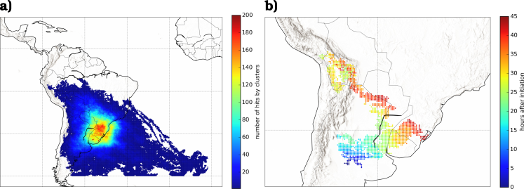
Figure 5: Family of rainfall clusters over subtropical South America. (a) The entire family of spatio-temporal clusters over subtropical South America. The colors indicate how often a given grid cell $i^{L}$ is hit by clusters in this family. This number is given by the number of nodes $n^{FL,i^{F}i^{L}}$ in supernode $V^{FL}_{i^{F}i^{L}}$ of the intersection partition $V^{FL}$. Note that the superscript $FL$ indicates that the supernodes $V^{FL}_{i^{F}i^{L}}$ arise from intersecting the partitions given by the types of features ‘family membership’ $F$ and ‘geographical label’ $L$. High values over southeastern South America therefore indicate that this is the core region of this family, where most of its clusters pass by in course of their lifetime. (b) Exemplary cluster of this family. Each colored grid cell has received at least one event above the $90$th percentile belonging to this cluster. The colors indicate the last time (in units of hours) a given grid cell is hit by the cluster, relative to its initiation on February 6, 2011, 18:00 UTC. The temporal evolution of this cluster therefore shows a concise propagation pattern from the Argentinean lowlands across Uruguay toward the eastern slopes of the Central Andes in Bolivia, where the clusters ends on February 8, 2011, 15:00 UTC. This cluster thus lasted for $\Delta t_{i}=45h$, and the total sum of water it precipitated was $v^{sum}_{i}=4.08\cdot 10^{10}m^{3}$, over a total area of $a^{sum}_{i}=9.39\cdot 10^{5}km^{2}$.

The second family [Fig. 6(a)] we want to show includes spatio-temporal clusters which exhibit equally concise propagation patterns in the tropical parts of South America. Similarly to the case described in the previous paragraph, we find several tropical clusters which propagate in the opposite direction of the climatological low-level wind fields. Some of these are initiated at the boundary between tropics and subtropics, move northward along the eastern slopes of the Peruvian Andes, before turning eastward toward the Amazonian lowlands [as for example the cluster shown in Fig. 6(b)]. Other instances form just east of the northern Andes, and roughly follow the equator toward the East [as for example the cluster shown in Fig. 6(c)]. In view of the above explanations for the first family, we speculate that similar mechanisms leading to the “upstream” propagation of favorable conditions for organized convection are at work in these cases. However, frontal systems do rarely reach these tropical latitudes Siqueira and Rossow (2005), and a saddle point similar to the one described above is not present in this case. While Amazonian squall lines, which propagate from the northern Brazilian coast into the continent, have been thoroughly analyzed Tulich and Kiladis (2012); Cohen et al. (1995), these organized spatio-temporal clusters moving northward along the tropical Andes and from West to East across the Amazon have – to our knowledge – not yet been studied in the meteorological and climatological literature. We therefore propose these particular spatio-temporal clusters as a promising subject for further research.

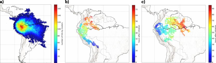
Figure 6: Family of rainfall clusters over tropical South America. (a) The entire family of spatio-temporal clusters over tropical South America. The colors indicate how often a given grid cell $i^{L}$ is hit by clusters in this family, given by $n^{FL,i^{F}i^{L}}$ [see the caption of Fig. 5(a)]. High values over the western Amazon therefore indicate that this the core region of this family, where most of its clusters pass by in course of their lifetime. (b) First exemplary cluster of this family. Each colored grid cell has received at least one event above the $90$th percentile belonging to this cluster. The colors indicate the last time (in units of hours) a given grid cell is hit by the cluster, relative to its initiation on November 4, 2002, 9:00 UTC. The temporal evolution of this cluster therefore shows a concise propagation pattern from central Bolivia northward, along the eastern slopes of the Andes mountain range, before turning west in northern Peru. The cluster ends on November 7, 2002, 15:00 UTC over Colombia and northwestern Brazil, resulting in a total lifetime of $\Delta t_{i}=78h$. The total sum of water precipitated by this cluster is $v^{sum}_{i}=4.90\cdot 10^{10}m^{3}$, covering a total area of $a^{sum}_{i}=1.53\cdot 10^{6}km^{2}$. (c) Second exemplary cluster of this family. It initiated on March 20, 2013, 18:00 UTC, at the eastern slopes of the northern Peruvian Andes, and thereafter propagated eastward across the entire Amazon basin, ending on March 24, 2013, 18:00 UTC over northern Brazil. During its lifetime of $\Delta t_{i}=96h$, the total sum of water precipitated by this cluster is $v^{sum}_{i}=1.17\cdot 10^{11}m^{3}$, covering a total area of $a^{sum}_{i}=2.61\cdot 10^{6}km^{2}$.

VI Conclusion

In this paper, we have introduced a collection of definitions resulting in deep graphs, a theoretical framework to describe and analyze heterogeneous systems across scales, based on network theory. Our framework unifies existing network representations and generalizes them by fulfilling two essential objectives: an explicit incorporation of information or data, and a comprehensive treatment of groups of objects and their relations. The former objective is implemented by specifying the nodes and edges of a (super)graph as sets of their respective properties. These properties, which may differ from node to node and from edge to edge, can be arbitrary mathematical objects. The second objective is implemented by transferring the mathematical concept of partition lattices to our graph representation. We have demonstrated how partitioning the node and edge set of a graph facilitates the means to aggregate, compute and allocate information on and between arbitrary groups of nodes. This information can then be stored on the lattices of a graph, allowing us to express and study properties, relations and interactions on all scales of the represented system(s).

Based on our representation, we were able to show how deep graphs establish an interface for common data analysis and modelling tools. This includes network-based concepts, models and methods, since we derived the different representations of a multilayer network Kivelä et al. (2014), which was the most general network representation to date.

Yet, we have also introduced additional tools to support a comprehensive data analysis. We have demonstrated how the auxiliary connector and selector functions enable us to create and select (super)edges, thereby allowing us to forge the topology of a deep graph. Intersection partitions not only allow us to derive a tensor-like representation of a multilayer network De Domenico et al. (2013), but they also allow us to calculate similarity measures between (intersection) partitions of a graph and to express elaborate queries on the information contained in a deep graph.

We have demonstrated some capabilities of our framework by applying it to a global high-resolution precipitation dataset derived from satellite measurements. Deep graphs provided a natural and straightforward way to identify large clusters of extreme precipitation events, track their temporal resolution, and group the resulting spatio-temporal clusters into families according to their regional overlap. We have furthermore discussed some climatological characteristics of two of these families over the South American continent. The first, which is concentrated over the subtropics, was just recently discovered using rather complicated methodologies, while the second, which is concentrated over tropical South America, has to our knowledge not yet been identified and analyzed in the meteorological literature.

The software package we provide in dee includes all the capabilities of our representation as described in this paper, and constitutes a powerful, general-purpose data analysis toolkit. Connector and selector functions can be defined by the user, which are then combined in order to efficiently create edges, where the number of CPUs and memory usage can be fully adjusted.

We hope that our framework initiates attempts to generalize existing network measures and to develop new measures, particularly in respect of the heterogeneity of a system’s components and their interactions on different scales. In the context of multilayer networks, generalizations of network measures have already led to significant new insights, and we expect the same to become true for deep graphs.

Appendix A Measuring the Similarity of (Intersection) Partitions

In this section, we demonstrate how the construction of intersection partitions provides us with the elements of a so-called confusion matrix (or contingency table). These are necessary to compute similarity measures between partitions, such as, e.g.: the Jaccard index Jaccard (1912); the normalized mutual information Strehl and Ghosh (2003); or the normalized variation of information metric Meilă (2007). First, we show how to compute the similarity of two “normal” partitions, and then how to compute the similarity of two intersection partitions.

Assume we are given a graph $G=(V,E)$ comprised of $n$ nodes, and two partitions of the node set, $V^{p}=\{V^{p}_{i}\;\vline\;i=1,2,...,n^{p}\}$ and $V^{p^{\prime}}=\{V^{p^{\prime}}_{i^{\prime}}\;\vline\;i^{\prime}=1,2,...,n^{p^{\prime}}\}$. The number of nodes in supernode $V^{p}_{i}$ ($V^{p^{\prime}}_{i^{\prime}}$) is then given by $n^{p,i}$ ($n^{p^{\prime},i^{\prime}}$), and the number of nodes in supernode $V^{p\cdot p^{\prime}}_{i\cdot i^{\prime}}$ of the intersection partition $V^{p\cdot p^{\prime}}$ is given by $n^{p\cdot p^{\prime},i\cdot i^{\prime}}$ [see Eqs. (27)-(29)]. With these numbers, we can calculate the normalized variation of information metric by

$$\text{NVI}=\dfrac{-1}{\log n}\sum_{i}\sum_{i^{\prime}}\dfrac{n^{p\cdot p^{\prime},i\cdot i^{\prime}}}{n}\log\dfrac{(n^{p\cdot p^{\prime},i\cdot i^{\prime}})^{2}}{n^{p,i}n^{p^{\prime},i^{\prime}}}.$$ (63)

Analogously, we can compute other similarity measures, such as the Jaccard index or the normalized mutual information index (see Eqs. (6) and (7) in Granell et al. (2015)).

More generally, we can compute the similarity of two intersection partitions. Assume we are given a graph $G=(V,E)$ comprised of $n$ nodes, and set of $K$ partitions of $V$, induced by a set of functions ${}^{v}p=\{{}^{v}p^{k}\;\vline\;k\in I^{K}\}$, where $I^{K}=\{1,2,...,K\}$ is the partition index set. From this set of available partitions, we choose two collections, $g\subseteq I^{K}$ and $g^{\prime}\subseteq I^{K}$, whose corresponding intersection partitions we want to compare. The number of nodes in supernode $V^{\underline{p}}_{\underline{i}}$ ($V^{\underline{p}^{\prime}}_{\underline{i}^{\prime}}$) is given by $n^{\underline{p},\underline{i}}$ ($n^{\underline{p}^{\prime},\underline{i}^{\prime}}$), and the number of nodes in supernode $V^{\underline{p}\cdot\underline{p}^{\prime}}_{\underline{i}\cdot\underline{i}^{\prime}}$ of the intersection partition $V^{\underline{p}\cdot\underline{p}^{\prime}}$ is given by $n^{\underline{p}\cdot\underline{p}^{\prime},\underline{i}\cdot\underline{i}^{\prime}}$ (where $\underline{p}=(p^{k})_{k\in g}$, $\underline{i}=(i^{k})_{k\in g}$, $\underline{p}^{\prime}=(p^{k})_{k\in g^{\prime}}$, $\underline{i}^{\prime}=(i^{k})_{k\in g^{\prime}}$, and $i^{k}\in\{1,2,...,n^{p^{k}}\}$). Using these numbers in Eq. (63), we can compute the similarity of two different intersection partitions.

Equivalently, we can use the numbers $m,m^{\underline{p},\underline{i}\underline{j},\underline{r}},m^{\underline{p}^{\prime},\underline{i}^{\prime}\underline{j}^{\prime},\underline{r}^{\prime}}$ and $m^{\underline{p}\underline{p}^{\prime},\underline{i}\underline{i}^{\prime}\underline{j}\underline{j}^{\prime},\underline{r}\underline{r}^{\prime}}$ (see Tab. 4) to calculate similarity measures between (intersection) partitions of the edge set. Furthermore, we can use a pair of (intersection) partitions of the node set, in order to compute the similarity of their corresponding edge set partitions.

Appendix B Expressing Supernodes (Superedges) by Features (Relations)

Here, we explicitly demonstrate how the information contained in a given graph $G=(V,E)$ is conserved when creating partitions, by expressing supernodes and superedges in terms of features and relations, respectively. Given a partition $V^{\underline{p}}$ of $V$ induced by $\underline{p}$ [see Eqs. (27)-(29)], the set of features contained in supernode $V^{\underline{p}}_{\underline{i}}$ is given by

$$F^{\underline{p}}_{\underline{i}}=\{F^{m}_{j}\;\vline\;j\in\{1,2,...,n\}\land m\in\{1,2,...,f_{j}\}\land\forall k\in g:{}^{v}p^{k}(V_{j})={}^{v}S^{k}_{i^{k}}\}.$$ (64)

To keep track of a features’ original node index, and to guarantee uniqueness of every single feature, we technically would have to write $(j,F^{m}_{j})$ for every feature. Yet, for ease of notation, we refrain from doing so. Next, we map each feature $F^{m}_{j}$ in $F^{\underline{p}}_{\underline{i}}$ onto its respective type,

$$t^{\underline{p}}_{\underline{i}}:F^{\underline{p}}_{\underline{i}}\rightarrow T^{\underline{p}}_{\underline{i}}=\{1,2,...,n^{\underline{p},\underline{i}}_{\text{types}}\},F^{m}_{j}\mapsto t^{\underline{p}}_{\underline{i}}(F^{m}_{j}):=T^{\underline{p}}_{\underline{i},t}\in T^{\underline{p}}_{\underline{i}},$$ (65)

such that $t^{\underline{p}}_{\underline{i}}(F^{l}_{j})=t^{\underline{p}}_{\underline{i}}(F^{m}_{k})$ for all pairs of features in $F^{\underline{p}}_{\underline{i}}$ that share the same type. We denote the number of distinct types of features in supernode $V^{\underline{p}}_{\underline{i}}$ by $n^{\underline{p},\underline{i}}_{\text{types}}$. Note that $0\leq n^{\underline{p},\underline{i}}_{\text{types}}\leq|F^{\underline{p}}_{\underline{i}}|$, where $n^{\underline{p},\underline{i}}_{\text{types}}=0$ either because the supernode $V^{\underline{p}}_{\underline{i}}$ does not exist, $n^{\underline{p},\underline{i}}=0$, or because all the nodes it contains have no features, $n^{\underline{p},\underline{i}}\geq 1$ and $V_{j}=\{j\}$ for all $V_{j}\in V^{\underline{p}}_{\underline{i}}$. If no pair of nodes in $V^{\underline{p}}_{\underline{i}}$ shares any type of feature, then $n^{\underline{p},\underline{i}}_{\text{types}}=|F^{\underline{p}}_{\underline{i}}|$. The function $t^{\underline{p}}_{\underline{i}}$ induces a partition $F^{\underline{p},T}_{\underline{i}}$ of $F^{\underline{p}}_{\underline{i}}$ into features of common type $F^{\underline{p},T}_{\underline{i},t}$, given by

$$F^{\underline{p},T}_{\underline{i},t}=\{F^{m}_{j}\;\vline\;j\in\{1,2,...,n\}\land m\in\{1,2,...,f_{j}\}\land\forall k\in g:{}^{v}p^{k}(V_{j})={}^{v}S^{k}_{i^{k}}\land t^{\underline{p}}_{\underline{i}}(F^{m}_{j})=T^{\underline{p}}_{\underline{i},t}\},$$ (66)

and $F^{\underline{p},T}_{\underline{i}}=\{F^{\underline{p},T}_{\underline{i},t}\;\vline\;t\in\{1,2,...,n^{\underline{p},\underline{i}}_{\text{types}}\}\}$. We denote the number of features of type $t$ in supernode $V^{\underline{p}}_{\underline{i}}$ by $n^{\underline{p},\underline{i}}_{\text{t}}:=|F^{\underline{p},T}_{\underline{i},t}|$. Hence, we can express a supernode $V^{\underline{p}}_{\underline{i}}$ as a set of sets of features of common type (and its index, to guarantee uniqueness of the supernodes),

$$V^{\underline{p}}_{\underline{i}}=\{\underline{i}\}\cup\{F^{\underline{p},T}_{\underline{i},t}\}_{t\in\{1,2,...,n^{\underline{p},\underline{i}}_{\text{types}}\}}.$$ (67)

Analogously, we can express superedges in terms of their edges’ constituent relations. Given a partition $E^{\underline{p}}$ of $E$ induced by $\underline{p}$ [see Eqs. (33)-(40)], the set of relations contained in superedge $E^{\underline{p}}_{\underline{i}\underline{j},\underline{r}}$ is given by

$$R^{\underline{p}}_{\underline{i}\underline{j},\underline{r}}=\{R^{m}_{uv}\;\vline\;\Phi^{e}(u,v)\land\Phi^{v}_{g^{s}}(u)\land\Phi^{v}_{g^{t}}(v)\land\Phi^{e}_{g^{r}}(u,v)\land m\in\{1,2,...,r_{uv}\}\}.$$ (68)

Again, to keep track of a relations’ original indices and to guarantee uniqueness, we technically have to write $((u,v),R^{m}_{uv})$ for every relation, which we omit for notational clarity. Next, we map every relation $R^{m}_{uv}$ in $R^{\underline{p}}_{\underline{i}\underline{j},\underline{r}}$ onto its respective type,

$$t^{\underline{p}}_{\underline{i}\underline{j},\underline{r}}:R^{\underline{p}}_{\underline{i}\underline{j},\underline{r}}\rightarrow T^{\underline{p}}_{\underline{i}\underline{j},\underline{r}}=\{1,2,...,m^{\underline{p},\underline{i}\underline{j},\underline{r}}_{\text{types}}\},R^{m}_{uv}\mapsto t^{\underline{p}}_{\underline{i}\underline{j},\underline{r}}(R^{m}_{uv}):=T^{\underline{p}}_{\underline{i}\underline{j},\underline{r},t}\in T^{\underline{p}}_{\underline{i}\underline{j},\underline{r}},$$ (69)

such that $t^{\underline{p}}_{\underline{i}\underline{j},\underline{r}}(R^{m}_{ij})=t^{\underline{p}}_{\underline{i}\underline{j},\underline{r}}(R^{n}_{kl})$ for all pairs of relations in $R^{\underline{p}}_{\underline{i}\underline{j},\underline{r}}$ that share the same type. We denote the number of distinct types of relations in superedge $E^{\underline{p}}_{\underline{i}\underline{j},\underline{r}}$ by $m^{\underline{p},\underline{i}\underline{j},\underline{r}}_{\text{types}}$. Again, $0\leq m^{\underline{p},\underline{i}\underline{j},\underline{r}}_{\text{types}}\leq|R^{\underline{p}}_{\underline{i}\underline{j}}|$, where $m^{\underline{p},\underline{i}\underline{j},\underline{r}}_{\text{types}}=|R^{\underline{p}}_{\underline{i}\underline{j}}|$ only if no pair of edges in $E^{\underline{p}}_{\underline{i}\underline{j},\underline{r}}$ shares any type of relation. The partition $R^{\underline{p},T}_{\underline{i}\underline{j},\underline{r}}$ of $R^{\underline{p}}_{\underline{i}\underline{j},\underline{r}}$ into relations of common type $R^{\underline{p},T}_{\underline{i}\underline{j},\underline{r},t}$ is therefore induced by the function $t^{\underline{p}}_{\underline{i}\underline{j},\underline{r}}$, where

$$R^{\underline{p},T}_{\underline{i}\underline{j},\underline{r},t}=\{R^{m}_{uv}\;\vline\;\Phi^{e}(u,v)\land\Phi^{v}_{g^{s}}(u)\land\Phi^{v}_{g^{t}}(v)\land\Phi^{e}_{g^{r}}(u,v)\land m\in\{1,2,...,r_{uv}\}\land t^{\underline{p}}_{\underline{i}\underline{j},\underline{r}}(R^{m}_{uv})=T^{\underline{p}}_{\underline{i}\underline{j},\underline{r},t}\},$$ (70)

and $R^{\underline{p},T}_{\underline{i}\underline{j},\underline{r}}=\{R^{\underline{p},T}_{\underline{i}\underline{j},\underline{r},t}\;\vline\;t\in\{1,2,...,m^{\underline{p},\underline{i}\underline{j},\underline{r}}_{\text{types}}\}\}$. We denote the number of relations of type $t$ in superedge $E^{\underline{p}}_{\underline{i}\underline{j},\underline{r}}$ by $m^{\underline{p},\underline{i}\underline{j},\underline{r}}_{\text{t}}:=|R^{\underline{p},T}_{\underline{i}\underline{j},\underline{r},t}|$. Therefore, a superedge $E^{\underline{p}}_{\underline{i}\underline{j},\underline{r}}$ can be expressed as a set of sets of relations of common type (and its index, to guarantee uniqueness of the superedges),

$$E^{\underline{p}}_{\underline{i}\underline{j},\underline{r}}=\{(\underline{i},\underline{j},\underline{r})\}\cup\{R^{\underline{p},T}_{\underline{i}\underline{j},\underline{r},t}\}_{t\in\{1,2,...,m^{\underline{p},\underline{i}\underline{j},\underline{r}}_{\text{types}}\}}.$$ (71)

Appendix C Summary of the Multilayer Network Representation

In the following, we summarize the representations of a multilayer network (MLN), as defined by Kivelä et al Kivelä et al. (2014), and refer to the original paper for a more detailed description. A multilayer network (MLN) is defined by a quadruplet $M=(V_{M},E_{M},V^{N},\bm{L})$, where the set of $N$ nodes is given by $V^{N}=\{1,2,...,N\}$. The multidimensional layer structure is given by a sequence of sets of elementary layers, $\bm{L}=\{L_{a}\}^{d}_{a=1}$, where each of the $d$ sets of elementary layers $L_{a}$ corresponds to an ‘aspect’ $a$ of the MLN (e.g., $L_{1}=\{\text{facebook},\text{twitter},...\}$ could be a set of categories of connections, and $L_{2}=\{\text{2010},\text{2011},...\}$ could be a set of time stamps, at which edges are present). A layer in the structure given by $\bm{L}$ is then a combination of elementary layers from all aspects, or in other words: an element of the set of all layers given by the Cartesian product $L_{1}\times\cdot\cdot\cdot\times L_{d}$. Each node can belong to any subset of the layers, and the set of all existing node-layer tuples (in short: node-layers) $(u,\bm{\alpha})$, where $u\in V^{N}$ and $\bm{\alpha}\in L_{1}\times\cdot\cdot\cdot\times L_{d}$, is denoted $V_{M}\subseteq V^{N}\times L_{1}\cdot\cdot\cdot\times L_{d}$. Edges are allowed between all such existing node-layers, hence the set of edges is given by $E_{M}\subseteq V_{M}\times V_{M}$.

The pair $G_{M}=(V_{M},E_{M})$, referred to as the ‘supra-graph’ of $M$, is a graph on its own, where nodes are, as the authors say, “labelled in a certain way”. The adjacency matrix of $G_{M}$ is referred to as the ‘supra-adjacency matrix’ representation of $M$, and constitutes one possible representation of a MLN. Defining weights for edges of $M$ on the underlying graph $G_{M}$ (by some function $w:E_{M}\rightarrow\mathbb{R}$) yields a weighted MLN.

Another representation of a MLN can be achieved by adjacency tensors De Domenico et al. (2013). Given a MLN $M=(V_{M},E_{M},V^{N},\bm{L})$ with $d$ aspects, one can represent it by an order-$2(d+1)$ adjacency tensor $A_{uv\bm{\alpha}\bm{\beta}}=A_{uv\alpha_{1}\beta_{1}...\alpha_{d}\beta_{d}}$, where an element $A_{uv\bm{\alpha}\bm{\beta}}$ has a value of $1$, if and only if $((u,\bm{\alpha}),(v,\bm{\beta}))\in E_{M}$, and a value of $0$ otherwise. As the authors of Kivelä et al. (2014) explain, the representation of a MLN by an adjacency tensor is technically only valid for node-aligned MLNs, where all layers contain all nodes, $V_{M}=V^{N}\times L_{1}\times\cdot\cdot\cdot\times L_{d}$. Yet, many tensor-based methods on MLNs have been successfully applied by filling layers with ‘empty’ node-layers (node-layers that are not adjacent to any other node-layer), yielding an artificial node-aligned structure of the MLN. However, one has to be very cautious in the calculation and interpretation of tensor-based measures, and account for the presence of empty node-layers in an appropriate way Kivelä et al. (2014). In the tensor-representation of MLNs, weights can be introduced by defining a weighted adjacency tensor $W_{uv\bm{\alpha}\bm{\beta}}$, where the value of each element determines the weight of an edge (for non-existing edges, the value is $0$ by convention).

Appendix D Discussion of Multilayer Networks

In this section, we first demonstrate the alternative representation of a multilayer network (MLN) by our framework, which is given by placing the additional information attributed to the layered structure of a MLN $M$ in the edges of $G=(V,E)$. Then, we show the advantages of the representation stated in the main text. For that matter, we create the subset of the partition lattice ${}^{G}L$ of $G\mathrel{\widehat{=}}M$ that is induced by the types of features of its constituent nodes, and show that it incorporates not only the alternative representation shown here, but several others, including a tensor-like representation. Lastly, we discuss the constraints imposed on our framework in order to represent a MLN, and explain how our framework solves the issues encountered in the representation of MLNs.

The alternative representation of $M=(V_{M},E_{M},V^{N},\bm{L})$ by $G=(V,E)$ is given by identifying each node $V_{i}=\{i\}\in V=\{V_{1},V_{2},...,V_{N}\}$ with a node $V^{N}_{i}\in V^{N}$, $V_{i}\mathrel{\widehat{=}}V^{N}_{i}$. Denoting the weight of an edge of a MLN by $w\left(((V^{N}_{i},\bm{\alpha}),(V^{N}_{j},\bm{\beta}))\right)\in\mathbb{R}$, an edge $E_{ij}\in E^{\prime}=\{E_{11},E_{12},...,E_{NN}\}$ is given by

$$E_{ij}=\{w\left(((V^{N}_{i},\bm{\alpha}),(V^{N}_{j},\bm{\beta}))\right)\;\vline\;((V^{N}_{i},\bm{\alpha}),(V^{N}_{j},\bm{\beta}))\in E_{M}\}=:\{R^{k}_{ij}\;\vline\;k\in\{1,2,...,r_{ij}\}\},$$ (72)

where $|E_{ij}|=r_{ij}$ is the number of types of relations from node $V_{i}$ to node $V_{j}$. Hence, the edge set $E$ corresponding to $E_{M}$ is given by $E=\{E_{ij}\;\vline\;i,j\in\{1,2,...,N\}\land E_{ij}\neq\varnothing\}$. By this representation, we can clearly see that a tuple $(\bm{\alpha},\bm{\beta})$ defines the type of relation of an edge in $E_{M}$,

$$t\left(((V^{N}_{i},\bm{\alpha}),(V^{N}_{j},\bm{\beta}))\right)=t\left(((V^{N}_{k},\bm{\gamma}),(V^{N}_{l},\bm{\delta}))\right)\longleftrightarrow(\bm{\alpha},\bm{\beta})=(\bm{\gamma},\bm{\delta}),$$ (73)

for all $V^{N}_{i},V^{N}_{j},V^{N}_{k},V^{N}_{l}\in V^{N}$, where $t$ is a function mapping an edge to its corresponding type, $t:E_{M}\rightarrow T=\{1,2,...,m_{\text{types}}\}$, with $m_{\text{types}}=(\prod^{d}_{a=1}|L_{a}|)^{2}$. Therefore, the number of types of relations between any pair of nodes in a MLN is bounded by $r_{ij}\leq m_{\text{types}}$.

Next, we partition the graph $G=(V,E)\mathrel{\widehat{=}}(V_{M},E_{M})$ described by Eqs. (49) and (50). For notational uniformity, we rewrite the features of the nodes in $V$ as outputs of partition functions $p=\{p^{N},p^{1},p^{2},...,p^{d}\}$, where

$$p^{N}:V\rightarrow V^{N},V_{i}\mapsto p^{N}(V_{i})=V^{N}_{i},$$ (74)

$$p^{a}:V\rightarrow L_{a},V_{i}\mapsto p^{a}(V_{i})=L_{a,i},a=1,2,...,d.$$ (75)

Based on the $(1+d)$ partitions induced by $p$, we can redistribute the information contained in the graph $G$ on a subset of the lattice ${}^{G}L^{f}\subseteq{}^{G}L$. This redistribution allows for several representations of the graph $G$, some of which we will demonstrate in the following. Let us denote the partition index set of $p$ by $I^{K}=\{N,1,2,...,d\}$. Then we can select a total of $I(K)=2^{(1+d)}$ distinct collections $g\subseteq I^{K}$, resulting in $|{}^{G}L^{f}|\leq I(K)$ supergraphs $G^{\underline{p}}=(V^{\underline{p}},E^{\underline{p}})\in{}^{G}L^{f}$, where ${}^{G}L^{f}=\{G^{\underline{p}}\;\vline\;g\in\mathcal{P}(I^{K})\}$ and $\underline{p}=(p^{k})_{k\in g}$.

Choosing $g=\{N\}$ leads to the supergraph $G^{p^{N}}=(V^{p^{N}},E^{p^{N}})$, where each supernode $V^{p^{N}}_{i}\in V^{p^{N}}$ corresponds to a node of the MLN, $V^{p^{N}}_{i}\mathrel{\widehat{=}}V^{N}_{i}$. Superedges $E^{p^{N}}_{ij}\in E^{p^{N}}$ with $i=j$ correspond to the coupling edges of a MLN. The one to one correspondence of the supergraph $G^{p^{N}}$ to the above, edge-based choice of $G$ justifies the statement that the representation $G$ of $M$ given in the main text is the preferred one, since it fully entails the above choice.

Choosing the group $g=\{1,2,...,d\}$ leads to the supergraph $G^{p^{1}\cdot\cdot\cdot p^{d}}=(V^{p^{1}\cdot\cdot\cdot p^{d}},E^{p^{1}\cdot\cdot\cdot p^{d}})$, where every supernode $V^{p^{1}\cdot\cdot\cdot p^{d}}_{i^{1}\cdot\cdot\cdot i^{d}}\in V^{p^{1}\cdot\cdot\cdot p^{d}}$ corresponds to a distinct layer of $M$, encompassing all its respective nodes. Superedges $E^{p^{1}\cdot\cdot\cdot p^{d}}_{i^{1}\cdot\cdot\cdot i^{d},j^{1}\cdot\cdot\cdot j^{d}}\in E^{p^{1}\cdot\cdot\cdot p^{d}}$ with either $(i^{a})_{a=1}^{d}=(j^{a})_{a=1}^{d}$ or $(i^{a})_{a=1}^{d}\neq(j^{a})_{a=1}^{d}$ correspond to collections of intra- and inter-layer edges of a MLN, respectively.

The last supergraph we want to exemplify is given by choosing $g=\{N,1,2,...,d\}=I^{K}$, resulting in the supergraph $G^{p^{N}\cdot p^{1}\cdot\cdot\cdot p^{d}}=(V^{p^{N}\cdot p^{1}\cdot\cdot\cdot p^{d}},E^{p^{N}\cdot p^{1}\cdot\cdot\cdot p^{d}})$. This supergraph corresponds one to one to the graph $G=(V,E)$, and therefore to the ‘supra-graph’ representation of $M$, given by the tuple $(V_{M},E_{M})$. The only difference is the indexing. The graph $G$ has an adjacency matrix-like representation, given by $E_{ij}\in E^{\prime}$. We say ‘like’, since $E^{\prime}$ is not a matrix, formally. An element of $E^{\prime}$ is either a real number, corresponding to the weight of the corresponding edge in $E_{M}$, or an empty set, meaning the edge does not exist. $G^{p^{N}\cdot p^{1}\cdot\cdot\cdot p^{d}}$, on the other hand, has a tensor-like representation, given by $E^{p^{N}\cdot p^{1}\cdot\cdot\cdot p^{d}}_{i^{N}\cdot i^{1}\cdot\cdot\cdot i^{d},j^{N}\cdot j^{1}\cdot\cdot\cdot j^{d}}\in E^{p^{N}\cdot p^{1}\cdot\cdot\cdot p^{d}}$. Again, formally, $E^{p^{N}\cdot p^{1}\cdot\cdot\cdot p^{d}}$ is not a tensor. An element of $E^{p^{N}\cdot p^{1}\cdot\cdot\cdot p^{d}}$ is either a real number, corresponding to the weight of the corresponding edge in $E_{M}$, or an empty set, if the edge does not exist. As mentioned in Sec. III.5, we can distinguish between a superedge that does not exist because at least one of the supernodes does not exist, $n^{p^{N}\cdot p^{1}\cdot\cdot\cdot p^{d},i^{N}\cdot i^{1}\cdot\cdot\cdot i^{d}}$ or $n^{p^{N}\cdot p^{1}\cdot\cdot\cdot p^{d},j^{N}\cdot j^{1}\cdot\cdot\cdot j^{d}}=0$, or because there is no superedge between existing supernodes, $n^{p^{N}\cdot p^{1}\cdot\cdot\cdot p^{d},i^{N}\cdot i^{1}\cdot\cdot\cdot i^{d}}$ and $n^{p^{N}\cdot p^{1}\cdot\cdot\cdot p^{d},j^{N}\cdot j^{1}\cdot\cdot\cdot j^{d}}=1$.

From the perspective of our framework, all representations $G^{\underline{p}}\in{}^{G}L$ are equivalent, in the sense that the information contained in $G$ is conserved under partitioning. There is no need to “flatten” the MLN represented by $G^{p^{N}\cdot p^{1}\cdot\cdot\cdot p^{d}}$ to obtain its supra-adjacency matrix representation $G$, and there is no loss of information about the aspects, as – according to Kivelä et al. (2014) – it is the case for MLNs represented by $M=(V_{M},E_{M},V^{N},\bm{L})$.

Let us now summarize the constraints we imposed on our framework, in order to represent a MLN. First, we had to restrict ourselves to the representation of one element of a deep graph. Allocating information on and between groups of nodes, as described in Sec. III.6, is not intended within the framework of MLNs. Then, we have to decide whether to put to information attributed to the layered structure of $M$ into the nodes of $G$, or the edges of $G$. There is no genuine separation of features and relations in a MLN. Furthermore, the weights of the edges of a MLN need to be restricted to real numbers (or possibly complex numbers). This poses several limitations. First, it is problematic to distinguish between edges with a weight of $0$ (e.g. an edge representing a time difference of $0$) and non-existing edges, since edges with weight $0$ do not exist by convention in MLNs. Yet, more importantly, we can not assign distributions of values to nodes or edges, let alone more complex mathematical objects. Another complication arises, when dealing with nodes that have more or less than $d$ aspects, or more generally speaking: when dealing with heterogeneous kinds of nodes. Although it is possible to represent nodes with different types of features by filling layers with ‘empty’ node-layers, the procedure is rather counter-intuitive and leads to a cluttered representation. In contrast, our framework provides the means to represent heterogeneous objects and their relations in a sparse and intuitive manner.

Table 4: Glossary. The symbol “#” reads: “number of”, and “IP” reads: “intersection partition”.

Explanation	Symbol	Given by	Properties
# nodes	$n$	$|V|$	$\geq 1$
# supernodes	$n^{p}$	$|V^{p}|$	$1\leq n^{p}\leq n$
# supernodes (IP)	$n^{\underline{p}}$	$|V^{\underline{p}}|$	$1\leq n^{\underline{p}}\leq n$
# nodes in supernode $i$	$n^{p,i}$	$|V^{p}_{i}|$	$1\leq n^{p,i}\leq n$
# nodes in supernode $\underline{i}$ (IP)	$n^{\underline{p},\underline{i}}$	$|V^{\underline{p}}_{\underline{i}}|$	$0\leq n^{\underline{p},\underline{i}}\leq n$
# types of features in supernode $\underline{i}$ (IP)	$n^{\underline{p},\underline{i}}_{\text{types}}$	$|T^{\underline{p}}_{\underline{i}}|$	$0\leq n^{\underline{p},\underline{i}}_{\text{types}}\leq|F^{\underline{p}}_{\underline{i}}|$
# features of type $t$ in supernode $\underline{i}$ (IP)	$n^{\underline{p},\underline{i}}_{t}$	$|F^{\underline{p},T}_{\underline{i},t}|$	$\leq n^{\underline{p},\underline{i}}$
# partition-specific types of features in supernode $\underline{i}$ (IP)	${}^{\underline{p}}n^{\underline{p},\underline{i}}_{\text{types}}$	allocation	$\geq 0$
# features in node $i$	$f_{i}$	$|V_{i}|$	$\geq 0$
# distinct types of features in $G$	$n_{\text{types}}$	$|T_{v}|$	$\geq 0$
# features of type $t$ in $G$	$n_{t}$	$|F^{p^{c},T}_{i,t}|$	$\leq n$
# edges	$m$	$|E|$	$\geq 0$
# superedges	$m^{p}$	$|E^{p}|$	$0\leq m^{p}\leq m$
# superedges (IP)	$m^{\underline{p}}$	$|E^{\underline{p}}|$	$0\leq m^{\underline{p}}\leq m$
# edges in superedge $(i,j)$	$m^{p,ij}$	$|E^{p}_{ij}|$	$0\leq m^{p,ij}\leq m$
# edges in superedge $(\underline{i},\underline{j},\underline{r})$ (IP)	$m^{\underline{p},\underline{i}\underline{j},\underline{r}}$	$|E^{\underline{p}}_{\underline{i}\underline{j},\underline{r}}|$	$0\leq m^{\underline{p},\underline{i}\underline{j},\underline{r}}\leq m$
# types of relations in superedge $(\underline{i},\underline{j},\underline{r})$ (IP)	$m^{\underline{p},\underline{i}\underline{j},\underline{r}}_{\text{types}}$	$|T^{\underline{p}}_{\underline{i}\underline{j},\underline{r}}|$	$0\leq m^{\underline{p},\underline{i}\underline{j},\underline{r}}_{\text{types}}\leq|R^{\underline{p}}_{\underline{i}\underline{j},\underline{r}}|$
# relations of type $t$ in supernode $(\underline{i},\underline{j},\underline{r})$ (IP)	$m^{\underline{p},\underline{i}\underline{j},\underline{r}}_{t}$	$|R^{\underline{p},T}_{\underline{i}\underline{j},\underline{r},t}|$	$\leq m^{\underline{p},\underline{i}\underline{j},\underline{r}}$
# partition-specific types of relations in superedge $(\underline{i},\underline{j},\underline{r})$ (IP)	${}^{\underline{p}}m^{\underline{p},\underline{i}\underline{j},\underline{r}}_{\text{types}}$	allocation	$\geq 0$
# relations in edge $(i,j)$	$r_{ij}$	$|E_{ij}|$	$\geq 0$
# distinct types of relations in $G$	$m_{\text{types}}$	$|R^{p^{c}}_{ij}|$	$\geq 0$
# relations of type $t$ in $G$	$m_{t}$	$|R^{p^{c},T}_{ij,t}|$	$\leq m$

- (1) “Big data and analytics,” http://www-01.ibm.com/software/data/bigdata/what-is-big-data.html, accessed: 2015-08-29.
- Jaynes (2005) E. T. Jaynes, The Mathematical Intelligencer 27, 83 (2005).
- Anderson (2003) T. Anderson, An Introduction to Multivariate Statistical Analysis, Wiley Series in Probability and Statistics (Wiley, 2003).
- Strogatz (1994) S. Strogatz, Nonlinear Dynamics and Chaos: With Applications to Physics, Biology, Chemistry, and Engineering, Advanced book program (Westview Press, 1994).
- Thiel et al. (2010) M. Thiel, J. Kurths, M. Romano, G. Károlyi, and A. Moura, Nonlinear Dynamics and Chaos: Advances and Perspectives, Understanding Complex Systems (Springer Berlin Heidelberg, 2010).
- Osborne and Rubinstein (1994) M. J. Osborne and A. Rubinstein, A Course in Game Theory (MIT Press, 1994) p. 352.
- Newman (2010) M. Newman, Networks: An Introduction (OUP Oxford, 2010) p. 784.
- Hastie et al. (2009) T. Hastie, R. Tibshirani, and J. Friedman, The Elements of Statistical Learning: Data Mining, Inference, and Prediction, Second Edition, Springer Series in Statistics (Springer, 2009).
- Bishop (2006) C. Bishop, Pattern Recognition and Machine Learning, Information Science and Statistics (Springer, 2006).
- Haykin (2009) S. Haykin, Neural Networks and Learning Machines, Neural networks and learning machines No. Bd. 10 (Prentice Hall, 2009).
- Vapnik (1998) V. Vapnik, Statistical learning theory, Adaptive and learning systems for signal processing, communications, and control (Wiley, 1998).
- Deng and Yu (2014) L. Deng and D. Yu, DEEP LEARNING: Methods and Applications, Tech. Rep. MSR-TR-2014-21 (2014).
- Bollobas (1998) B. Bollobas, Modern Graph Theory (Springer Science & Business Media, 1998) p. 394.
- Horvath (2014) S. Horvath, Weighted Network Analysis: Applications in Genomics and Systems Biology (Springer New York, 2014).
- Wiedermann et al. (2013) M. Wiedermann, J. F. Donges, J. Heitzig, and J. Kurths, EPL (Europhysics Letters) 102, 28007 (2013).
- Berge (1976) C. Berge, Graphs and Hypergraphs, Graphs and Hypergraphs (North-Holland Publishing Company, 1976).
- Asratian et al. (1998) A. Asratian, T. Denley, and R. Häggkvist, Bipartite Graphs and Their Applications, Cambridge Tracts in Mathematics (Cambridge University Press, 1998).
- Boccaletti et al. (2014) S. Boccaletti, G. Bianconi, R. Criado, C. I. Del Genio, J. Gómez-Gardeñes, M. Romance, I. Sendiña-Nadal, Z. Wang, and M. Zanin, Physics Reports 544, 1 (2014).
- Kivelä et al. (2014) M. Kivelä, A. Arenas, M. Barthelemy, J. P. Gleeson, Y. Moreno, and M. A. Porter, Journal of Complex Networks 2, 203 (2014).
- Berlingerio et al. (2011) M. Berlingerio, M. Coscia, F. Giannotti, A. Monreale, and D. Pedreschi, Proceedings - 2011 International Conference on Advances in Social Networks Analysis and Mining, ASONAM 2011 , 485 (2011).
- Han (2012) J. Han, in Proceedings of the 18th ACM SIGKDD International Conference on Knowledge Discovery and Data Mining, KDD ’12 (ACM, New York, NY, USA, 2012) pp. 2–3.
- De Domenico et al. (2013) M. De Domenico, A. Solé-Ribalta, E. Cozzo, M. Kivelä, Y. Moreno, M. A. Porter, S. Gómez, and A. Arenas, Physical Review X 3, 041022 (2013).
- Gao et al. (2011a) J. Gao, S. V. Buldyrev, H. E. Stanley, and S. Havlin, Nature Physics 8, 40 (2011a).
- Gao et al. (2011b) J. Gao, S. V. Buldyrev, S. Havlin, and H. E. Stanley, Physical Review Letters 107, 1 (2011b), arXiv:1010.5829 .
- Santiago and Benito (2008) A. Santiago and R. Benito, EPL (Europhysics Letters) 82, 58004 (2008).
- (26) “The DeepGraph Python Package,” https://github.com/deepgraph/deepgraph/, accessed: 2016-03-30.
- (27) “PyData Ecosystem - Downloads,” http://pydata.org/downloads/, accessed: 2015-08-29.
- Buluç et al. (2013) A. Buluç, H. Meyerhenke, I. Safro, P. Sanders, and C. Schulz, CoRR abs/1311.3144 (2013).
- Newman and Girvan (2004) M. Newman and M. Girvan, Physical Review E 69, 026113 (2004).
- Lucas (1990) J. F. Lucas, Introduction to Abstract Mathematics (Rowman & Littlefield, 1990) p. 382.
- Birkhoff (1940) G. Birkhoff, Lattice Theory, Volume 25, Part 2 (American Mathematical Soc., 1940) p. 418.
- Bell (1938) E. T. Bell, Annals of Mathematics Second Series, 39, pp. 539 (1938).
- Becker and Riordan (1948) H. W. Becker and J. Riordan, American Journal of Mathematics 70, pp. 385 (1948).
- Welsh (2010) D. Welsh, Matroid Theory, Dover books on mathematics (Dover Publications, 2010).
- Commons (2015) W. Commons, “The 15 partitions of a 4-element set ordered in a Hasse diagram,” https://commons.wikimedia.org/wiki/File:Set_partitions_4;_Hasse;_circles.svg (2015), accessed: 2015-08-29.
- Granell et al. (2015) C. Granell, R. K. Darst, A. Arenas, S. Fortunato, and S. Gómez, Physical Review E 92, 012805 (2015).
- Boers et al. (2013) N. Boers, B. Bookhagen, N. Marwan, J. Kurths, and J. Marengo, Geophysical Research Letters 40, 4386 (2013).
- Zhou et al. (2006) C. Zhou, L. Zemanová, G. Zamora, C. C. Hilgetag, and J. Kurths, Phys. Rev. Lett. 97, 238103 (2006).
- Aicher et al. (2013) C. Aicher, A. Z. Jacobs, and A. Clauset, arXiv preprint arXiv:1305.5782 (2013).
- Peixoto (2012) T. P. Peixoto, Physical Review E 85, 056122 (2012).
- Peixoto (2013) T. P. Peixoto, Physical Review Letters 110, 148701 (2013).
- Peixoto (2014) T. P. Peixoto, Physical Review X 4, 011047 (2014).
- Campanharo et al. (2011) A. S. Campanharo, M. I. Sirer, R. D. Malmgren, F. M. Ramos, and L. A. N. Amaral, PloS one 6, e23378 (2011).
- Marwan (2008) N. Marwan, The European Physical Journal Special Topics 164, 3 (2008).
- Marwan and Kurths (2002) N. Marwan and J. Kurths, Physics Letters, Section A: General, Atomic and Solid State Physics 302, 299 (2002).
- Huffman et al. (2007) G. J. Huffman, D. T. Bolvin, E. J. Nelkin, D. B. Wolff, R. F. Adler, G. Gu, Y. Hong, K. P. Bowman, and E. F. Stocker, Journal of Hydrometeorology 8, 38 (2007).
- Stolbova et al. (2014) V. Stolbova, P. Martin, B. Bookhagen, N. Marwan, and J. Kurths, Nonlinear Processes in Geophysics 21, 901 (2014).
- Boers et al. (2014) N. Boers, B. Bookhagen, H. M. J. Barbosa, N. Marwan, J. Kurths, and J. Marengo, Nature Communications 5:5199 (2014), doi:10.1038/ncomms6199.
- Field et al. (2012) C. B. Field, V. Barros, T. F. Stocker, D. Qin, D. J. Dokken, K. L. Ebi, M. D. Mastrandrea, K. J. Mach, S. K. Allen, and M. Tignor, in Managing the Risks of Extreme Events and Disasters to Advance Climate Change Adaptation - A Special Report of Working Groups I and II of the Intergovernmental Panel on Climate Change (IPCC) (2012) pp. 555–564.
- Sokal et al. (1958) R. Sokal, C. Michener, and U. of Kansas, A Statistical Method for Evaluating Systematic Relationships, University of Kansas science bulletin (University of Kansas, 1958).
- Vera et al. (2006) C. Vera, W. Higgins, J. Amador, T. Ambrizzi, R. D. Garreaud, D. Gochis, D. Gutzler, D. Lettenmaier, J. A. Marengo, C. R. Mechoso, J. Nogues-Paegle, P. Silva Dias, and C. Zhang, Journal of Climate 19, 4977 (2006).
- Marengo et al. (2012) J. A. Marengo, B. Liebmann, A. M. Grimm, V. Misra, P. L. Silva Dias, I. F. A. Cavalcanti, L. M. V. Carvalho, E. H. Berbery, T. Ambrizzi, C. S. Vera, Others, P. L. S. Dias, A. C. Saulo, J. Nogues-paegle, E. Zipser, A. Seth, and L. M. Alves, International Journal of Climatology 32, 1 (2012).
- Anabor et al. (2008) V. Anabor, D. J. Stensrud, and O. L. L. de Moraes, Monthly Weather Review 136, 3087 (2008).
- Boers et al. (2015) N. Boers, H. M. J. Barbosa, B. Bookhagen, J. a. Marengo, N. Marwan, and J. Kurths, Journal of Climate 28, 7641 (2015).
- Maddox (1980) R. A. Maddox, Bulletin of the American Meteorological Society 61, 1374 (1980).
- Durkee et al. (2009) J. D. Durkee, T. L. Mote, and J. M. Shepherd, Journal of Climate 22, 4590 (2009).
- Durkee and Mote (2009) J. D. Durkee and T. L. Mote, International Journal of Climatology 30, 418 (2009).
- Siqueira and Rossow (2005) J. Siqueira and W. Rossow, Monthly Weather Review 133, 1045 (2005).
- Tulich and Kiladis (2012) S. N. Tulich and G. N. Kiladis, Journal of the Atmospheric Sciences 69, 2995 (2012).
- Cohen et al. (1995) J. C. P. Cohen, M. A. F. S. Silva Dias, and C. A. Nobre, Monthly Weather Review 123, 3163 (1995).
- Jaccard (1912) P. Jaccard, New phytologist 11, 37 (1912).
- Strehl and Ghosh (2003) A. Strehl and J. Ghosh, J. Mach. Learn. Res. 3, 583 (2003).
- Meilă (2007) M. Meilă, Journal of multivariate analysis 98, 873 (2007).