Radioactive Iron Rain:
Transporting ${}^{60}{\rm Fe}$ in Supernova Dust to the Ocean Floor

Abstract

Several searches have found evidence of ${}^{60}{\rm Fe}$ deposition, presumably from a near-Earth supernova (SN), with concentrations that vary in different locations on Earth. This paper examines various influences on the path of interstellar dust carrying ${}^{60}{\rm Fe}$ from a SN through the Heliosphere, with the aim of estimating the final global distribution on the ocean floor. We study the influences of magnetic fields, angle of arrival, wind and ocean cycling of SN material on the concentrations at different locations. We find that the passage of SN material through the mesosphere/lower thermosphere (MLT) is the greatest influence on the final global distribution, with ocean cycling causing lesser alteration as the SN material sinks to the ocean floor. SN distance estimates in previous works that assumed a uniform distribution are a good approximation. Including the effects on surface distributions, we estimate a distance of $46^{+10}_{-6}$ pc for a $8-10\ M_{\odot}$ SN progenitor. This is consistent with a SN occurring within the Tuc-Hor stellar group $\sim$2.8 Myr ago with SN material arriving on Earth $\sim$2.2 Myr ago. We note that the SN dust retains directional information to within $1^{\circ}$ through its arrival in the inner Solar System, so that SN debris deposition on inert bodies such as the Moon will be anisotropic, and thus could in principle be used to infer directional information. In particular, we predict that existing lunar samples should show measurable ${}^{60}{\rm Fe}$ differences.

KCL-PH-TH/2016-15, LCTS/2016-09, CERN-TH-2016-076

1. Introduction

Supernovae (SNe) are some of the most spectacular explosions in our Galaxy. Occurring at a rate of $\sim$$1-3$ per century in the Milky Way (e.g., Adams et al., 2013, and references therein), it is likely that one (if not more) has exploded close enough to have produced detectable effects on the Earth. Speculation on biological effects of a near-Earth SN has a long history in the literature (e.g., Shklovskii, 1968; Alvarez et al., 1980; Ellis & Schramm, 1995), and Ellis et al. (1996) and Korschinek et al. (1996) proposed using radioactive isotopes such as ${}^{60}{\rm Fe}$ and ${}^{244}{\rm Pu}$ to find direct evidence of such an event. Although several studies have searched for ${}^{244}{\rm Pu}$, this paper will focus exclusively on ${}^{60}{\rm Fe}$. For more recent examinations of ${}^{244}{\rm Pu}$, see Wallner et al. (2000, 2004) and Wallner et al. (2015a).

With this motivation, Knie et al. (1999) examined a sample of ferro-manganese (Fe-Mn) crust from Mona Pihoa in the South Pacific and found an anomaly in ${}^{60}{\rm Fe}$ concentration that suggested a SN occurred near Earth sometime within the last 5 Myr (a specific time could not be determined). The study was later expanded in Knie et al. (2004) using a different Fe-Mn crust sample from the equatorial Pacific Ocean floor, and found a distinct signal in ${}^{60}{\rm Fe}$ abundance $\sim 2.2$ Myr ago, with a ${}^{60}{\rm Fe}$ fluence, ${\cal F}$, at the time of arrival calculated to have been ${\cal F}_{\rm Knie}=1.41\times 10^{6}\ {\rm atoms\ cm^{-2}}$. Fitoussi et al. (2008) subsequently confirmed the detection by Knie in the Fe-Mn crust, but did not find a corroborating signal in sea sediment samples from the northern Atlantic Ocean. Fitoussi et al. noted several reasons for the discrepancy, including variations in the background and differences in the uptake efficiencies between the Fe-Mn crust and sediment. An excess of ${}^{60}{\rm Fe}$ has also been found in lunar regolith samples (Cook et al., 2009; Fimiani et al., 2012, 2014, 2016) but, due to the nature of the regolith, only the presence of a signal is detectable, not the precise arrival time or fluence (Feige et al., 2013). Subsequently, results from Eltanin sediment samples from the southern Indian Ocean were reported in Feige (2014), confirming the Knie et al. (2004) Fe-Mn crust detection in these sea sediment samples and leading to an estimated arrival fluence of ${\cal F}_{\rm Feige}=1.42\times 10^{7}\ {\rm atoms\ cm^{-2}}$. This fluence is an order of magnitude higher than found by Knie et al. (2004), and the difference in fluence values was attributed to differences in uptake efficiencies for sea sediment versus Fe-Mn crust. Feige (2014) and Feige et al. (2013) noted that, whilst the sea sediment uptake efficiency is most likely $U_{\rm sediment}\approx 100\%$, other observations (including the recent, extensive study of ${}^{60}{\rm Fe}$ measurements by Wallner et al., 2016) suggest the Fe-Mn crust has an uptake efficiency of $U_{\rm crust}\in[0.1,1]$.

Complementing the multiple searches for ${}^{60}{\rm Fe}$ and other isotopes, several papers have discussed the interpretations and implications of the ${}^{60}{\rm Fe}$ signal. The hydrodynamic models used by Fields et al. (2008) discussed the interaction of a SN blast with the solar wind, and highlighted the necessity (see also Athanassiadou & Fields, 2011) of ejecta condensation into dust grains capable of reaching Earth. Fry et al. (2015) examined the possible sources of the Knie ${}^{60}{\rm Fe}$ signal, finding an Electron-Capture SN (ECSN), with Zero-Age Main Sequence (ZAMS) mass $\approx 8-10\ M_{\odot}$ (“$\odot$” refers to the Sun), to be the most likely progenitor, while not completely ruling out a Super Asymptotic Giant Branch (SAGB) star with ZAMS mass $\approx 6.5-9\ M_{\odot}$.

With regards to a possible location of the progenitor, Benítez et al. (2002) suggested that the source event for the ${}^{60}{\rm Fe}$ occurred in the Sco-Cen OB association. This association was $\sim$130 pc away at the time of the ${}^{60}{\rm Fe}$-producing event, and its members were described in detail by Fuchs et al. (2006). Breitschwerdt et al. (2012) modeled the formation of the Local Bubble with a moving group of stars (approximating the Sco-Cen association) and plotted their motion in the Milky Way at 5-Myr intervals for the past 20 Myr (see Figure 9 of Breitschwerdt et al., 2012). More recently, Breitschwerdt et al. (2016) have expanded this examination using hydrodynamic simulations to model SNe occurring within the Sco-Cen association and track the ${}^{60}{\rm Fe}$ dust entrained within the blast. Additionally, Kachelrieß et al. (2015) and Savchenko et al. (2015) found a signature in the proton cosmic ray spectrum suggesting an injection of cosmic rays associated with a SN occurring $\sim$2 Myr ago, and Binns et al. (2016) found ${}^{60}{\rm Fe}$ cosmic rays, suggesting a SN origin within the last $\sim 2.6$ Myr located $\lesssim 1$ kpc of Earth, based on the ${}^{60}{\rm Fe}$ lifetime and cosmic ray diffusion. With particular relevance for our discussion, Mamajek (2016) suggested the Tuc-Hor group could have provided an ECSN to produce the ${}^{60}{\rm Fe}$. The group was within $\sim$60 pc of Earth $\sim$2.2 Myr ago and, given the masses of the current group members, could well have hosted a star with a ZAMS mass $\geq 8M_{\odot}$.

Fry et al. (2015) noted that these and other studies assumed a uniform deposition of ${}^{60}{\rm Fe}$ material over Earth’s entire surface, and proposed that the direction of arriving material and the Earth’s rotation could shield portions of Earth’s surface from SN material. Since ${}^{60}{\rm Fe}$ dust from a SN would be arriving along one direction instead of isotropically, the suggestion was that certain portions of Earth’s surface would face the SN longer than others and collect more arriving material. This could explain why the northern Fitoussi et al. (2008) sediment samples showed no obvious signal, whereas the southern Feige et al. (2013), Feige (2014) sediment samples showed a stronger signal than the equatorial Knie et al. (2004) crust sample.

This paper re-examines that possibility, and studies how the angle of arrival of dust from a SN effects the deposition on the Earth’s surface. We show that the dust propagation in the inner Solar System introduces deflections of order a few degrees. Thus, the angle of arrival drastically changes the received fluence at the top of the Earth’s atmosphere. However, any such variations are lost as the SN material descends through our atmosphere, and the final global distribution is due primarily to atmospheric influences with slight alterations due to ocean cycling. This confirms an isotropic deposition on the Earth’s surface as a reasonable assumption when making order of magnitude calculations. This in turn removes an uncertainty in estimates of the distance to the ${}^{60}{\rm Fe}$ progenitor, which may have been within the Sco-Cen or Tuc-Hor stellar groups.

In contrast, the memory of the angle of arrival would be retained in deposits on airless Solar System bodies such as the Moon. We find that lunar samples should show significant variation in SN ${}^{60}{\rm Fe}$ abundance if the source was in the Tuc-Hor or the Sco-Cen groups. Thus the ${}^{60}{\rm Fe}$ pattern on the Moon in principle can give directional information, serving as a low-resolution “antenna” that could potentially test proposed source directions.

Lastly, our examination assumes the passage of a single SN. In studying Solar System/terrestrial influences on SN ${}^{60}{\rm Fe}$, we find that none are capable of extending the signal postulated by Fry et al. (2015) to the wider signal detected by Feige (2014) and Wallner et al. (2016). This supports the assertion by Breitschwerdt et al. (2016) and Wallner et al. (2016) of multiple SNe producing the ${}^{60}{\rm Fe}$ signal.

2. Motivation

Fry et al. (2015) defined the decay-corrected fluence as that measured at the time the signal arrived. However, inherent in the formula used in Fry et al. (2015) (and in all other studies known to us) was the assumption that the material was distributed uniformly, that is, isotropically, over Earth’s entire surface. Here we examine this assumption in detail. In fact, the arriving SN blast will be highly directional, roughly a plane wave on Solar System scales (Fields et al., 2008).

In this paper, we will assume that all SN dust will be entrained in the blast plasma as it arrives in the Solar System. That is, we ignore any relative motion of the dust in the blast. Thus the dust will arrive with the same velocity vector as the blast. The SN dust particles will then encounter the blast/solar wind interface, decouple, and be injected into the Solar System with a plane-wave geometry.

As SN dust traverses the Solar System, it passes through magnetic fields, multiple layers of the Earth’s atmosphere and water currents until finally being deposited on the ocean floor. In addition, because we would expect dust from a SN to arrive as a plane wave as the Earth rotates, different regions would have become exposed to the wave for different durations. Relaxing the assumption of uniformly distributed debris deposition gives:

$${\cal F}({\it lat,lon}) =\psi({\it lat,lon})$$

$$\times\left(\frac{1}{4}\right)\left(\frac{M_{\rm ej}}{4\pi D^{2}Am_{u}}\right)\ Ufe^{-t_{\rm travel}/\tau}\,,$$ (1)

where ${\cal F}({\it lat,lon})$ is the fluence of the isotope at the time the signal arrives at a location with latitude and longitude $({\it lat,lon})$ on Earth’s surface. Here $M_{\rm ej}$ is the mass of the ejected isotope, $D$ is the distance the isotope travels from the SN to Earth, $A$ is the atomic mass of the isotope, $m_{u}$ is the atomic mass unit, $U$ is the uptake efficiency of the material the isotope is sampled from, $f$ is the fraction of the isotope in the form of dust that reaches Earth, $t_{\rm travel}$ is the time taken by the isotope to travel from the SN to Earth, and $\tau$ is the mean lifetime of the isotope. The factor of $\nicefrac{{1}}{{4}}$ comes from the ratio of Earth’s cross-section to its surface area, and the factor $4\pi$ assumes spherical symmetry in the SN’s expansion. The uptake efficiency is a measure of how readily a material incorporates the elements deposited on it. Sediment accepts nearly all deposited elements, so we assume $U_{\rm sediment}=1$. However, the Fe-Mn crust incorporates iron through a chemical leaching process, so the uptake for iron into the crust is thought to lie in the range $U_{\rm crust}\approx 0.1-1$ (for more discussion, see Feige et al., 2012; Feige, 2014; Fry et al., 2015; Wallner et al., 2016). In order to account for concentrations and dilutions in the deposition of SN material, we include a factor $\psi$ to represent the deviation from a uniform distribution $(\psi=1)$, where $\psi\in[0,\ 1)$ implies a diluted deposition and $\psi>1$ implies a concentrated deposition.

When we compare samples from different terrestrial locations, most of the quantities in Equation (1) disappear, so that the fluence ratios depend only on the uptake and distribution factors:

$$\frac{{\cal F}_{\rm Fitoussi}}{{\cal F}_{\rm Knie}} =\frac{\left(\frac{\psi_{\rm Fitoussi}}{4}\right)\left(\frac{M_{\rm ej}}{4\pi D^{2}Am_{u}}\right)U_{\rm Fitoussi}fe^{-t_{\rm travel}/\tau}}{\left(\frac{\psi_{\rm Knie}}{4}\right)\left(\frac{M_{\rm ej}}{4\pi D^{2}Am_{u}}\right)U_{\rm Knie}fe^{-t_{\rm travel}/\tau}}$$

$$=\frac{U_{\rm Fitoussi}\psi_{\rm Fitoussi}}{U_{\rm Knie}\psi_{\rm Knie}}\,.$$ (2)

Similarly:

$$\frac{{\cal F}_{\rm Fitoussi}}{{\cal F}_{\rm Feige}}=\frac{U_{\rm Fitoussi}\psi_{\rm Fitoussi}}{U_{\rm Feige}\psi_{\rm Feige}}\,,$$ (3)

$$\frac{{\cal F}_{\rm Feige}}{{\cal F}_{\rm Knie}}=\frac{U_{\rm Feige}\psi_{\rm Feige}}{U_{\rm Knie}\psi_{\rm Knie}}\,.$$ (4)

Using these relations, we can test a distribution model against observations.

3. ${}^{60}{\rm Fe}$ Fluence Observations

We examine three studies of ${}^{60}{\rm Fe}$ measurements: Knie et al. (2004), Fitoussi et al. (2008), and Feige (2014). These studies have considerable overlap in their time periods and greatly varying locations on the Earth. We do not examine the Wallner et al. (2016) measurements in detail, first, because the bulk of the analysis for this paper was completed and submitted for review prior to the publication of Wallner et al. (2016), and second, because many of the samples included in Wallner et al. (2016) are either already included in the other studies, do not cover the period around the 2.2-Myr signal, or were drawn from similar latitudes as the other samples.

Table 1Model Cases, Uptakes, and Fluences

Case	$U_{\rm crust}$	$U_{\rm sediment}$
High Uptake	1	1
Medium Uptake	0.5	1
Low Uptake	0.1	1
${\cal F}_{\rm Knie}$	${\cal F}_{\rm Fitoussi}$	${\cal F}_{\rm Feige}$
$(1.41\pm 0.49)\times 10^{6}$	$\leq 1.1\times 10^{8}$	$(1.42\pm 0.37)\times 10^{7}$

Fluences are given in atoms cm^-2

3.1. Knie et al. (2004) Sample

The Knie et al. (2004) study used the hydrogenous deep-ocean Fe-Mn crust 237KD from 9^∘18’ N, 146^∘03’ W ($\sim$1,600 km/1,000 mi SE of Hawaii). The crust growth rate is estimated at 2.37 mm Myr^-1 (Fitoussi et al., 2008), and samples were taken at separations corresponding to 440- and 880-kyr time intervals. Knie et al. originally estimated that the ${}^{60}{\rm Fe}$ signal occurred 2.8 Myr ago with a decay-corrected fluence of $(2.9\pm 1.0)\times 10^{6}\ {\rm atoms\ cm^{-2}}$. However, at the time of their analysis, the half-life of ${}^{60}{\rm Fe}$ was estimated to be 1.49 Myr, and the half-life of ${}^{10}{\rm Be}$ (which was used to date individual layers) was estimated to be 1.51 Myr. Current best estimates for these values are $\tau_{1/2\text{, \mbox{${}^{60}{\rm Fe}$}}}=2.60$ Myr (Rugel et al., 2009; Wallner et al., 2015b) and $\tau_{1/2\text{, \mbox{${}^{10}{\rm Be}$}}}=1.387$ Myr (Chmeleff et al., 2010; Korschinek et al., 2010). This changes the estimated signal arrival time to 2.2 Myr ago, and gives a decay-corrected fluence of ${\cal F}_{\rm Knie}=(1.41\pm 0.49)\times 10^{6}\ {\rm atoms\ cm^{-2}}$. Additionally, Knie et al. used an iron uptake efficiency of $U_{\rm crust}=0.006$, whereas more recent studies suggest that the uptake for the crust is much higher, $U_{\rm crust}\approx 0.1-1$ (Bishop & Egli, 2011; Feige, 2014; Wallner et al., 2016). In this paper, we consider a “Medium” case that uses the Knie fluence of ${\cal F}_{\rm Knie}=(1.41\pm 0.49)\times 10^{6}\ {\rm atoms\ cm^{-2}}$ and an uptake of $U_{\rm crust}=0.5$, but we also examine the possibilities that the uptake is higher ($U_{\rm crust}=1$) and lower ($U_{\rm crust}=0.1$). Of special note, Feige (2014) and Wallner et al. (2016) found $U_{\rm crust}\in[0.07,0.17]$; both studies assumed an isotropic terrestrial distribution and found $U_{\rm crust}\approx 0.1$ by comparing crust and sediment fluences. Because the sediment samples came from the Indian Ocean, and the crust samples came from the Pacific and Atlantic Oceans, the distribution factor could potentially be pertinent, so we consider a range of $U_{\rm crust}$ values.

3.2. Fitoussi et al. (2008) Samples

Fitoussi et al. (2008) performed measurements on both Fe-Mn crust and sea sediment. The Fitoussi crust sample came from the same Fe-Mn crust used by Knie et al. (2004), but from a different section of it. The Fitoussi sea sediment samples are from 66^∘56.5’ N, 6^∘27.0’ W in the North Atlantic ($\sim$400 km/250 mi NE of Iceland). The average sedimentation rate for the samples is 3 cm kyr^-1, and slices were made corresponding to time intervals of $10-15$ kyr. The sediment samples had a density 1.6 g cm^-3 and an average iron weight fraction 0.5 wt%. Fitoussi et al. (2008) examined the period $1.68-3.2$ Myr ago, but found no significant ${}^{60}{\rm Fe}$ signal above the background level like that found in the Knie crust sample (Figure 3, Fitoussi et al., 2008). In an effort to further analyze their results, they calculated the running means for the samples using data intervals of $\sim$400 and 800 kyr (Figure 4, Fitoussi et al., 2008). This allowed the narrower sediment time intervals to be compared to the longer crust time intervals. They also considered the lowest observed sample measurement as the background level, rather than the total mean value used initially. In this instance, they found a signal of marginal significance in the 400-kyr running mean centered at $\sim$2.4 Myr of ${}^{60}{\rm Fe}$/Fe$=(2.6\pm 0.8)\times 10^{-16}$.

For this paper, we consider as part of our “Medium” scenario a non-detection by Fitoussi et al. (2008) (in other words, ${\cal F}_{\rm Fitoussi}=0\ {\rm atoms\ cm^{-2}}$). In addition, we assume an upper limit set by non-detection of a signal in the Fitoussi et al. (2008) sediments because of a high sedimentation rate. This is motivated by initial Fitoussi et al. (2008) measurements that found a slightly elevated ${}^{60}{\rm Fe}$ abundance at $\sim$2.25 Myr ago, but were not significant because they were not sufficiently above the background (Fitoussi et al., 2008). To determine this upper limit, we first calculate the number density of iron in the sediment (Feige et al., 2012):

$$n_{\rm Fe}=\frac{wN_{A}\rho}{A}\,,$$ (5)

where $w=0.005$ is the weight fraction of iron in the samples, $N_{A}$ is Avogadro’s number, $\rho=1.6\ {\rm g\ cm^{-3}}$ is the mass density of the sample, and $A=55.845\ {\rm g\ mol^{-1}}$ is the molar mass for iron. This yields a number density of $n_{\rm Fe}=8.6\times 10^{19}\ {\rm atoms\ cm^{-3}}$. Using the marginally significant signal to calculate the ${}^{60}{\rm Fe}$ number density, we find $n_{\text{\mbox{${}^{60}{\rm Fe}$}}}=8.6\times 10^{19}\ {\rm atoms\ cm^{-3}}\cdot 2.6\times 10^{-16}=2.2\times 10^{4}\ {\rm atoms\ cm^{-3}}$. An 870-kyr time interval (in order to compare to the fluence quoted by Knie et al. (2004) corresponds to a length of 2610 cm, and gives an upper limit on the fluence of $5.9\times 10^{7}\ {\rm atoms\ cm^{-2}}$. Correcting for radioactive decay gives the following upper limit on the fluence at the time the signal arrived:

$${\cal F}_{\rm Fitoussi}\leq\frac{5.9\times 10^{7}\ {\rm atoms\ cm^{-2}}}{2^{-2.2\ {\rm Myr}/2.60\ {\rm Myr}}}$$

$$\Rightarrow\qquad {\cal F}_{\rm Fitoussi}\leq 1.1\times 10^{8}\ {\rm atoms\ cm^{-2}}\,.$$ (6)

3.3. Feige (2014) Samples

Feige (2014) studied four sea sediment samples from the South Australian Basin in the Indian Ocean (1,000 km/620 mi SW of Australia). Three of the sediment cores cover the time period examined by Knie et al. (2004) and Fitoussi et al. (2008): ELT45-21 (39^∘00.00’ S, 103^∘33.00’ E), ELT49-53 (37^∘51.57’ S, 100^∘01.73’ E) and ELT50-02 (39^∘57.47’ S, 104^∘55.69’ E). They have an average density of 1.35 g cm^-3, an average iron weight fraction of 0.2 wt%, and sedimentation rates of 4 mm kyr^-1 for ELT45-21 and ELT50-02 and 3 mm kyr^-1 for ELT49-53. Feige (2014) studied samples from $0-4.5$ Myr ago, primarily in the time period of the Knie signal and was able to corroborate it, finding a decay-corrected fluence ${\cal F}_{\rm Feige}=(1.42\pm 0.37)\times 10^{7}\ {\rm atoms\ cm^{-2}}$. For our “Medium” scenario, we adopt the Feige (2014) fluence and assume that the uptake for sediment (for both the Fitoussi et al. (2008) and Feige (2014) samples) is $U_{\rm sediment}=1$. In our model comparisons, we use the location of the ELT49-53 sample. Table 1 summarizes the assumptions we use in our modeling.

4. Deposit Considerations

Table 2Maximum Trajectory Deflection for Various Grain Parameters

Grain Charge (V)	Speed (km s-1)	Grain Radius ($\mu$m)	$\beta$	IMF Deflection (∘)	Magnetosphere Deflection (∘)	Reaches Earth
5	40	0.2	0.8	0.5	0.04	Yes
0.5	40	0.2	0.8	0.3	0.005	Yes
50	40	0.2	0.8	5	0.4	Yes
5	40	0.02	0.1	3	5	Yes
5	40	2	0.1	0.3	0.02	Yes
5	20	0.2	0.8	0.9	0.07	No
5	80	0.2	0.8	0.4	0.02	Yes

As noted above, in this paper we assume that the dust grains are entrained within the SN shock until it reaches the Heliosphere, at which time the dust grains decouple from the shock and enter the Solar System, where they are affected by the magnetic fields present. Apart from the Sun’s magnetic, gravitational, and radiative influences, we consider only Earth’s magnetic and gravitational influences and ignore those of other objects in the Solar System (e.g., the Moon, Jupiter, etc.). We describe the dust with fiducial values of grain radius $a\geq 0.2\ \mu$m, charge corresponding to a voltage ${\cal V}=5$ V, and initial velocity $v_{\rm grain,0}\geq 40$ km s^-1.

4.1. Magnetic Deflection

The grains will experience a number of forces upon entering the Solar System: drag from collisions with the solar wind, radiation pressure from sunlight, gravity from the Sun and Earth, and a Lorentz force from magnetic fields since the grains will most likely be charged. Athanassiadou & Fields (2011) studied these effects in detail for SN grains, though with somewhat different SN parameters than are now favored, primarily due to the possible large revisions in crust uptake values. Nevertheless, following Athanassiadou & Fields (2011), we expect the influence of magnetic fields to be the dominant force for most of the grains traveling through interplanetary space. With our fiducial SN dust properties, we would not expect drag from the solar wind to affect the dust grains significantly, given that the drag stopping distance $R_{\rm drag}$ is much larger than the size of the Solar System (Murray et al., 2004):

$$R_{\rm drag}=1.7\ {\rm pc}\left(\frac{\rho_{\rm grain}}{3.5\ {\rm g\ cm^{-3}}}\right)\left(\frac{a}{0.2\ \mu{\rm m}}\right)\left(\frac{7.5\ {\rm cm^{-3}}}{n_{\rm H}}\right)\,.$$ (7)

The remaining forces (gravitational, radiation, and magnetic) have comparable values.

As noted in Fry et al. (2015), for a ratio of the Sun’s radiation force ($F_{\rm rad}$) to its gravitational force ($F_{\rm grav}$), $\beta\lesssim 1.3$, the dust grains will reach Earth’s orbit:

$$\beta\equiv\frac{F_{\rm rad}}{F_{\rm grav}}=0.8 \left(\frac{C_{\rm r}}{7.6\times 10^{-5}\ {\rm g\ cm}^{-2}}\right)\left(\frac{Q_{\rm pr}}{1}\right)$$

$$\times \left(\frac{3.5\ {\rm g\ cm}^{-3}}{\rho_{\rm grain}}\right)\left(\frac{0.2\ {\rm\mu m}}{a}\right)\,,$$ (8)

where $C_{\rm r}$ is a constant and $Q_{\rm pr}$ is the efficiency of the radiation pressure on the grain (for more detail see Gustafson, 1994).

The field strength of the interplanetary magnetic field (IMF, generated by the Sun) varies from a value of $B\sim 0.1\ \mu$G at 100 AU to $B\sim 50\ \mu$G at 1 AU. This implies the ratio of the magnetic to gravitational force varies over a range that is at least $F_{\rm mag}/F_{\rm grav}\approx 0.03-2$:

$$\frac{F_{\rm mag}}{F_{\rm grav}}=2 \left(\frac{\cal V}{5\ {\rm V}}\right)\left(\frac{B}{0.3\ \mu{\rm G}}\right)\left(\frac{v}{40\ {\rm km\ s^{-1}}}\right)$$

$$\times \left(\frac{r}{100\ {\rm AU}}\right)^{2}\left(\frac{3.5\ {\rm g\ cm}^{-3}}{\rho_{\rm grain}}\right)\left(\frac{0.2\ {\rm\mu m}}{a}\right)^{2}\,.$$ (9)

Both the IMF and the Magnetosphere (generated by the Earth) have similar strengths at the surfaces of their respective sources ($B\sim 1$ G), that weaken rapidly further away. Beyond 1 AU, the IMF is less than 100 $\mu$G, likewise the tail portion of the Magnetosphere asymptotically approaches 100 $\mu$G. Because the Sun’s radiation and gravitational forces are of similar magnitude, but opposite directions, we can estimate the influence of magnetic fields on the incoming SN dust grains before the in-depth numerical discussion below. If we calculate the gyroradius for our fiducial grain values, we get (Murray et al., 2004):

$$R_{\rm mag}=28\ {\rm AU} \left(\frac{\rho_{\rm grain}}{3.5\ {\rm g\ cm^{-3}}}\right)\left(\frac{5\ {\rm V}}{\cal V}\right)\left(\frac{100\ \mu{\rm G}}{B}\right)$$

$$\times \left(\frac{v_{\rm grain,0}}{40\ {\rm km\ s^{-1}}}\right)\left(\frac{a}{0.2\ \mu{\rm m}}\right)^{2}\,.$$ (10)

Given the sizes of the Solar System ($\sim$100 AU) and the Magnetosphere ($\sim$1000 $R_{\oplus}$, “$\oplus$” refers to the Earth), we would expect some deflection by the IMF, though not a complete disruption since the IMF weakens by several orders of magnitude beyond 1 AU, whereas the Magnetosphere should cause very little deflection of the dust grains. The numerical results below confirm this expectation, as summarized in Table 2.

4.1.1 Heliosphere Transit

The IMF has a shape resembling an Archimedean spiral due to a combination of a frozen-in magnetic field, the Sun’s rotation, and an outward flowing solar wind (Parker, 1963). At Earth’s orbit, the IMF has a value of $\vec{B}_{r,\theta,\phi}=\left<30,0,30\right>\ \mu$G (Gustafson, 1994), with the azimuthal component dominating at larger radii (Parker, 1958). Athanassiadou & Fields (2011) studied the passage of SN dust grains through the IMF, and calculated their deflection, but for velocities $\geq 100$ km s^-1. In this section we expand on Athanassiadou & Fields’s treatment by looking at slower initial grain velocities and solving numerically the equations of motion for the dust grain.

$$m_{\rm grain}\frac{d\vec{v}_{\rm grain}}{dt}=\vec{F}_{\rm grav,\odot}+\vec{F}_{\rm rad,\odot}+\vec{F}_{\rm mag,\odot}$$ (11)

We include the Lorentz force, $\vec{F}_{\rm mag,\odot}$, due to the IMF as well as the Sun’s gravity, $\vec{F}_{\rm grav,\odot}$, and radiation, $\vec{F}_{\rm rad,\odot}$, forces. Grain erosion is not included since the erosion timescale is much longer than the crossing time for the grains; neither are changes in grain charge since we expect the charge remains fairly constant once it enters the Solar System (Kimura & Mann, 1998). Our results are in good agreement with the broader and more detailed examination completed by Sterken et al. (2012, 2013)

The grains begin 110 AU from the Sun and have initial velocities directed at a location 1 AU away from the Sun representing Earth. We vary the initial grain directions, speeds, charges, and sizes, and solve for the angle between the grain’s initial direction and the line between the grain’s starting location and closest approach to Earth’s location. For our fiducial grain values, they experienced $\lesssim 1^{\circ}$ of deflection, and, since their velocities were greater than the solar escape velocity, they continued out of the Solar System after passing Earth’s orbit. Additionally, when examined as a plane wave, the grains showed a fairly uniform deflection amongst neighboring grains until closest approach, meaning that, even though a grain that was initially aimed at Earth would miss by $\sim 1^{\circ}$, another neighboring grain would be deflected into the Earth. These results suggest that direction information of the grains’ source would be retained to within $1^{\circ}$, and that spatial and temporal dilutions/concentrations of the ${}^{60}{\rm Fe}$ signal can be ignored, see Figure 1.

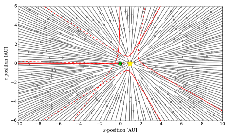
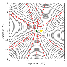
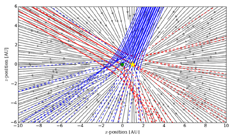
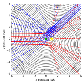
Figure 1.— Sample dust grain trajectories within the Heliosphere. The magnetic field lines are shown with grey arrows, the Sun is shown by a yellow star at $(1,0,0)$ AU, and the Earth is shown by a green $\oplus$ at the origin (NOTE: the Sun and Earth sizes are not to scale). Dust grain trajectories are shown in red or blue with the incoming trajectory indicated by solid lines, and, after closest approach to Earth, the outgoing trajectory is indicated by dashed lines. The initial dust grain parameters are: $a=0.2\ \mu$m, ${\cal V}=5$ V, and $v=40$ km s^-1. The upper panel shows individual dust grain trajectories initially aimed at Earth and how they behave in the inner Solar System. The lower panel shows a dust swarm with grains initially travelling parallel to each other, and grains not initially aimed at Earth can be deflected into it.

4.1.2 Earth’s Magnetosphere Transit

The Earth’s Magnetosphere has a teardrop shape, with field lines on the day-side being compressed by solar wind pressure on the plasma frozen in the Magnetosphere, and being stretched on the night-side nearly parallel to one another. The day-side edge is located $\sim$10 $R_{\oplus}$ with a field strength about twice that of the dipole value (§6.3.2, Kivelson & Russell, 1995). The night-side tail extends out to $\sim$1000 $R_{\oplus}$ with a radius of $\sim$30 $R_{\oplus}$ (§9.3, Kivelson & Russell, 1995). It reaches asymptotically a field strength $B_{X0}\approx 100\ \mu$G (Slavin et al., 1985) and has a current sheet half-height of $H=R_{\oplus}/2$ (Tsyganenko, 1989). We use the Magnetosphere approximation from Katsiaris & Psillakis (1987); this model is a superposition of a dipole field ($\vec{B}_{\rm dipole}$) near Earth (Dragt, 1965) and an asymptotic sheet ($\vec{B}_{\rm tail}$) for the magnetotail region (Wagner et al., 1979). This approximation does not include the inclination of the dipole field to the orbital plane but, given the motion and flipping of the magnetic poles, this approximation should suffice for examining general properties. We assume a magnetic dipole strength based on the equatorial surface value of $M\approx 1\ {\rm G}\ R_{\oplus}^{3}$, and assume that the tail magnetic field normal component $B_{Z0}\approx 0.06B_{X0}$ (Slavin et al., 1985). When we solve the equations of motion (Equation (11) adding the Lorentz force due to the Magnetosphere, $\vec{F}_{\rm mag,\oplus}$, and Earth’s gravity, $\vec{F}_{\rm grav,\oplus}$) for a charged particle in a magnetic field starting at various locations at the edge of the Magnetosphere moving towards the Earth, we find deflections are $\lesssim 3$ arcmin when using our fiducial grain values. Like the IMF, the grains show uniform deflections passing through the Magnetosphere, suggesting that direction information of the grains’ source would be retained to within $10$ arcmin, and that spatial and temporal dilutions/concentrations of the ${}^{60}{\rm Fe}$ signal can be ignored, see Figure 2.

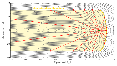
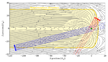
Figure 2.— Sample dust grain trajectories within the Magnetosphere. The magnetic field lines are shown with grey arrows, the Earth is shown (to scale) by a green $\oplus$ at the origin, and the boundary of the Magnetosphere is shown with a yellow line (NOTE: Magnetic field lines outside of the boundary were not used and can be ignored). Dust grain trajectories are shown in red or blue with the initial locations indicated by dots, the incoming trajectory indicated by solid lines, and, after closest approach to Earth, the outgoing trajectory is indicated by dashed lines. The initial dust grain parameters are: $a=0.2\ \mu$m, ${\cal V}=5$ V, and $v=40$ km s^-1. The left panel shows that individual dust grain trajectories initially aimed at Earth experience little deflection and impact Earth. The right panel shows a dust swarm with grains initially travelling parallel to each other remain parallel until after passing Earth.

4.2. Upper Atmosphere Distribution

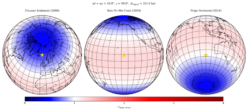
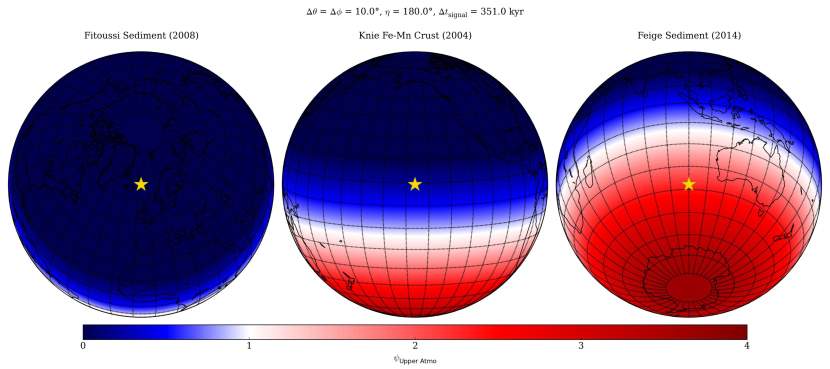
Figure 3.— Sample values of the distribution factor, $\psi$, as a function of the arrival angle, $\eta$ at the top of the atmosphere. As $\eta$ increases from $\eta=0^{\circ}$, the distribution changes from a northern concentration to an equatorial concentration at $\eta=90^{\circ}$. The sampling locations are shown as yellow stars in the centers of the figures. Note that, regardless of the value of $\eta$, the equator always receives some flux. It should be noted that the plotting program used to make these figures automatically smooths the transition from grid to grid, making the figures appear of higher resolution than actually calculated. However, based on the latitudinally-averaged values, the grid-to-grid transitions are, in fact, smooth, and the appearance shown in the figure is accurate.

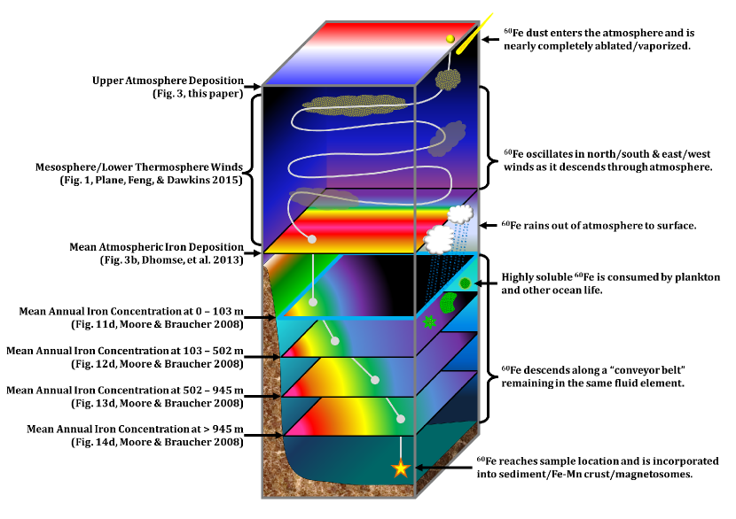
Figure 4.— Schematic of ${}^{60}{\rm Fe}$ passage through the atmosphere to the ocean floor. This diagram summarizes the processes and assumptions outlined in §4.2-4.4. On the left side of the diagram, the relevant references used in tracking the ${}^{60}{\rm Fe}$ material’s passage are given, and on the right side, the main processes acting on the ${}^{60}{\rm Fe}$ material are described. Color gradients indicate concentration gradients of iron and mimic those found in the source figures referenced at left. For this schematic, the colors of the gradients do not have specific values associated with them, but show how the referenced figures relate to one another. A SN dust grain containing ${}^{60}{\rm Fe}$ enters at the top of the schematic, is vaporized, and the ${}^{60}{\rm Fe}$ vapor descends through the atmosphere until it is rained out to the surface. This surface location is given in Fig. 3b, Dhomse et al. (2013), and the ${}^{60}{\rm Fe}$ material will enter the ocean fluid element at the corresponding location in Fig. 11d, Moore & Braucher (2008); in this schematic, the fluid element has a “green” concentration. The ${}^{60}{\rm Fe}$ remains in this “green” fluid element as it descends; the location of the “green” fluid element in Fig. 14d, Moore & Braucher (2008) will correspond to the sampling location on the ocean floor. To determine the amount of wind and water deflection, we follow the ${}^{60}{\rm Fe}$ material’s path backwards from the sampling location, along the fluid element with the associated iron concentration to the surface, and to the accompanying location on Fig. 3b, Dhomse et al. (2013).

Once the SN dust has passed through the IMF and Magnetosphere, it impacts the upper atmosphere (generally at $\sim$100 km in altitude, see §4.3). Because the IMF and Magnetosphere show little deflection, we expect a relatively coherent, nearly plane-wave flow of incident dust onto Earth’s upper atmosphere. Once the grains reach Earth, they will impinge onto Earth’s cross-section facing the dust wave. The upper atmosphere distribution will depend on Earth’s rotation and precession and the angle of arrival of the dust (see Figure 3). To find the dust distribution in the upper atmosphere where the SN material impacts and before it begins to pass through the rest of the atmosphere, we approximate the Earth as a perfect sphere that rotates about the $z$-axis. We divide the surface of the Earth into sectors of angular size $\Delta\theta\times\Delta\phi$, with $\theta$ and $\phi$ analogous to latitude and longitude, respectively. Because the duration of the SN dust storm is likely to be long ($\Delta t_{\rm signal}\sim 100$ kyr), we include Earth’s axial precession ($\Delta t_{\rm precessional}=26$ kyr). We ignore nutation of Earth’s axis, since it is small ($\sim$arcseconds) compared to the Earth’s inclination ($\alpha\approx 23.3^{\circ}$). Because the SN progenitor is far away ($D>10$ pc), we assume the direction of the particle flux does not change with time and its intensity is uniform, so we ignore Earth’s change in position through its orbit. We also assume that the SN dust intensity varies with time according to the saw-tooth pattern used in Fry et al. (2015): the initial flux ($\mathbb{F}_{0}$) starts at a maximum and decreases linearly to 0 at $t=\Delta t_{\rm signal}$.

In order to determine the fluence received at a given location on Earth, we use a series of coordinate transformations from the Earth’s surface/terrestrial (unprimed) frame to the propagating shock wave/interstellar (^′′′′) frame. For a detailed description of our transformations, see Appendix A.

Our simulations were run assuming a SN signal duration of $\Delta t_{\rm signal}=351$ kyr (the approximate expected duration for an ECSN, Fry et al., 2015). Because $\Delta t_{\rm signal}>\Delta t_{\rm precession}$, the model showed little dependence on the signal duration after the first precession cycle (terrestrial models were run for the entire SN signal width: 351 kyr; lunar models were run for four precession cycles: 74 yr). The same is true for a constant flux profile versus a saw-tooth profile. Because the model includes two vastly different time scales (precessional and daily), we used two different time steps. The precessional time steps were made when the precession progressed by an angle $\Delta\phi/2$. In other words:

$$\Delta t_{\rm precessional~{}step}=\left(\frac{26\ {\rm kyr}}{360^{\circ}}\right)\left(\frac{\Delta\phi}{2}\right)\,.$$ (12)

At each precessional time step, the model is run for one daily rotation, with the daily time steps made when the daily rotation progresses by an angle $\Delta\phi/2$, or:

$$\Delta t_{\rm daily~{}step}=\left(\frac{86400\ {\rm s}}{360^{\circ}}\right)\left(\frac{\Delta\phi}{2}\right)\,.$$ (13)

Precession still occurs during the daily time steps, but the effects of the daily rotation dominate. As we ran our model, the various angles $\eta$ represent different arrival directions from the source of the ${}^{60}{\rm Fe}$ signal as measured from the Ecliptic North Pole. Because of Earth’s precession and rotation, these possible directions form a ring of constant Ecliptic latitude.

Figure 3 shows sample results for our upper atmosphere distribution model, and we can see for the $\eta=90^{\circ}$ case, there is a nearly isotropic distribution of particles onto the entire atmosphere; $\psi_{\rm Upper~{}Atmo,~{}\eta=90^{\circ}}\in[0.5,\ 1.2]$. As $\eta$ increases to 180^∘, the North Pole becomes increasingly depleted ($\psi\rightarrow 0$), and the South Pole becomes increasingly saturated (the $\eta\in[0,\ 90^{\circ})$ case mirrors this result). At $\eta=180^{\circ}$, the saturation reaches a maximum; $\psi_{\rm Upper~{}Atmo,~{}\eta=180^{\circ}}\in[0,\ 3.7]$.

We see in Figure 3 that the arrival distribution of SN material is uniform across longitudes (i.e., constant at a fixed latitude). This arises primarily due to the daily rotation, with some additional smearing due to precessional rotation. Conversely, the distribution of SN dust on the upper atmosphere is strongly nonuniform across latitudes. The latitude gradient largely reflects the direction of the SN itself, with some smearing due to precession. As we will see, the fate of this SN signature is very different for the Earth and Moon.

4.3. Wind Deflection

Interstellar dust containing ${}^{60}{\rm Fe}$ could be subject to two types of wind effects: initial deflection through the atmosphere and subsequent transplantation from a landmass into the ocean. Since the solar wind has little influence on the SN dust grains, they would enter Earth’s atmosphere at approximately the same speed they entered the Solar System: $v_{\rm SN\ grains}\approx 40-100$ km s^-1. Although this is faster than typical meteoritic dust infall velocities, we would expect SN dust to be ablated at similar altitudes to meteoritic dust because both are traveling supersonically relative to the surrounding air and the stopping distance is independent of the initial velocity: in the supersonic limit, the $e$-folding stopping distance for dust grains is independent of their initial velocity (Murray et al., 2004). This implies that the SN dust grains would come to rest relative to the atmosphere in the upper mesosphere/lower thermosphere (MLT, $\sim$$90-115$ km above sea level, Feng et al., 2013). However, because of their high velocities, we would expect the SN grains to be completely ablated upon impact with the atmosphere, and thus vaporized. At this point, the SN ${}^{60}{\rm Fe}$ vapor would descend through the atmosphere (see Figure 4).

We expect that the SN dust grains and meteoritic dust grains would be similar in size ($a\sim 0.1-1\ \mu$m), so their ablation and fragmentation properties would also be similar. The SN grains would be ablated at altitudes similar to where meteoric grains are ablated, and both would descend through the atmosphere in a similar manner. Their compositions (iron oxides and silicates) are identical, so both SN and meteoritic materials would experience similar chemical reactions in the atmosphere. Because of these similarities, we use the extensive work already accomplished on meteoric smoke particles (e.g., Plane et al., 2015, and references therein).

Once delivered to the MLT, the SN material would sediment out to the surface over the course of $4-6$ years (Dhomse et al., 2013). As noted in §4.2, because of Earth’s rotation and precession, the upper atmosphere distribution forms bands of uniform fluences across lines of latitude. Since zonal (east-west) deflection would not affect that pattern, we focus on deflections due to meridional (north-south) winds. In the MLT, meridional winds are of the order $v_{\rm MLT\ winds}\sim 10$ m s^-1 and can be several orders of magnitude greater than the vertical component (Figure 1, Plane et al., 2015). These winds could drive the SN material from one pole to the other within a few days while descending only a few kilometers. An example of this movement was the plume from the launch of STS-107 on January 16, 2003: within $\sim$80 hr the plume had traveled from the eastern coast of Florida to the Antarctic (Niciejewski et al., 2011). Downward transport through the mesosphere-stratosphere-troposphere occurs mainly in the polar regions: this leads to a semi-annual oscillation of meteoritic smoke particles from pole to pole that would effectively isotropize (or at least randomize) the distribution of incoming SN material in the mesosphere.

Table 3Summary of Dust Grain Transit Through Solar System to Ocean Floor

Region	Primary Influences	Residence Time	Characteristic Region Boundary*
Interplanetary	IMF, Solar Radiation/Gravity	$\sim 10-12$ years	$100-150$ AU
Magnetosphere	Terrestrial Magnetic Field	$\lesssim 2$ days	$10-1000\ R_{\oplus}$
Upper Atmosphere (MLT)	Collisional Drag/Ablation & Strong Winds	$4-6$ years	$90-115$ km
Troposphere	Rain, Wind	$1-2$ weeks	$\sim 10$ km
Surface:
- Land	Transplantation by Surface Winds	indefinite	$\sim$ km
- Water	Biological Uptake, Ocean Currents	$100-200$ years	$\sim 4$ km
Ocean Floor	Biological Transplantation/Disturbance	indefinite	$\sim$ m
* - Boundary distances are measured from Earth’s surface except for the Water and Ocean Floor regions which are measured from the ocean floor.

In addition, the vaporized SN ${}^{60}{\rm Fe}$ would be highly soluble and would combine with sulphates as it descended through the stratosphere (Dhomse et al., 2013). This means the SN material would be readily incorporated into clouds when it finally reaches the troposphere (Saunders et al., 2012). Because the SN ${}^{60}{\rm Fe}$ would behave similarly to meteoritic iron, we can use simulations of the meteoritic smoke particles to find the final distribution of SN ${}^{60}{\rm Fe}$ at the surface. Dhomse et al. (2013) studied the transport of ${}^{238}{\rm Pu}$ through the atmosphere and later applied their model to iron deposition, finding the distribution over the entire Earth, with asymmetries in the mid-latitudes due to the stratosphere-troposphere exchange (see Figure 3b, Dhomse et al., 2013).

After descending through the atmosphere, it is possible for interstellar dust grains that have fallen through the atmosphere and been deposited on land to later be picked up by wind again, carried to the ocean, and be deposited there. This process of dust transplantation (also called aeolian dust), could lead to an enhancement of ${}^{60}{\rm Fe}$ levels in ocean samples. In the case of our studied samples, however, this should not be an issue. Based on a study by Jickells et al. (2005), aeolian iron dust deposits are low in the area of the Knie et al. (2004) and Feige (2014) samples. While slightly higher than the other locations, the Fitoussi et al. (2008) sample should not be affected because of where the dust was transplanted from. In the case of the Fitoussi sediment samples, the material will be transplanted from equatorial regions (e.g., to the Sahara, Arabian, and Gobi deserts), but as described in (see Figure 3b, Dhomse et al., 2013), these areas will receive very little SN material so we would expect the transplanted dust to contain a negligible amount of SN ${}^{60}{\rm Fe}$. Therefore, for the purposes of this paper we ignore dust transplantation, but future studies should consult Jickells et al. (2005) to check if transplantation is an issue.

Table 4Predicted Fluence Ratios for Uptake Values

$\psi_{\rm Knie}=0.43$, $\psi_{\rm Fitoussi}=0.14$, $\psi_{\rm Feige}=1.4$
Fluence Ratios	Observed	High Uptake	Medium Uptake	Low Uptake
${\cal F}_{\rm Fitoussi}/{\cal F}_{\rm Knie}=$	$0.\ (<70.9)$	0.33	0.65	3.3
${\cal F}_{\rm Fitoussi}/{\cal F}_{\rm Feige}=$	$0.\ (<7.04)$	0.11	0.11	0.11
${\cal F}_{\rm Feige}/{\cal F}_{\rm Knie}=$	$10.\pm 6$	3.3	6.5	33

4.4. Water Deflection

As mentioned in §4.3, the SN material would be highly soluble due to its complete ablation in the MLT. This means that when it reached the ocean it would be incorporated readily into organisms, particularly phytoplankton (Boyd & Ellwood, 2010). In many locations, the availability of iron is the limiting factor for phytoplankton growth (Figure 7, Moore et al., 2004). In locations where there is an abundance of iron (i.e., high concentrations of soluble iron, most likely due to meteoric or aeolian sources, and iron is not the limiting element), the residence time for iron is very short ($\sim$days and months), but in locations of lower abundance of Fe, the residence time is longer ($\sim$$100-200$ years) (Bruland et al., 1994; Croot et al., 2004). In either case, these residence times are much less than the ocean circulation time ($\sim$1000 years).

When quantifying the distribution of iron as it descends in the ocean, a number of considerations need to be included, not only the initial location of iron, the water velocity and its depth, but also the complexation of iron with organic ligands, the availability of other nutrients such as phosphates and nitrates, seasonal patterns, ocean floor topography, and the amount of light exposure. Several studies have examined iron cycling in the ocean (see e.g., LefèVre & Watson, 1999; Archer & Johnson, 2000; Parekh et al., 2004; Dutkiewicz et al., 2005, 2012). However, all of these studies examine the total iron input into oceans, the dominant source being aeolian dust which is highly insoluble, rather than meteoritic sources that are highly soluble but account for only $10^{-4}$ of the total iron input mass (Jickells et al., 2005; Plane, 2012).

A more recent study by Moore & Braucher (2008) examined the global cycling of iron and updated the Biogeochemical Elemental Cycling (BEC) ocean model, resulting in an improved model that showed better agreement with observations. As part of this study, Moore & Braucher simulated the concentrations of dissolved iron at varying ocean depths; of particular interest are the simulations of “Only Dust” inputs (see Figures 11d, 12d, 13d, and 14d, Moore & Braucher, 2008). While the dust used in the simulation is primarily from an aeolian source, it acts similarly to meteoric dust (or interstellar SN dust) upon reaching the ocean. Since the residence time of iron is much less than the ocean circulation time, we can approximate the ocean currents as “conveyor belts”, moving different concentrations of iron to different areas of the ocean, but not significantly altering the concentration of a fluid element as it descends. With this assumption, we can find a first-order, initial location of the dust input by looking at the iron concentration over each ${}^{60}{\rm Fe}$ sampling location in the lowest depths (Figure 14d, Moore & Braucher, 2008) and following it back to its source on the surface (Figure 11d, Moore & Braucher, 2008). With this initial location, we can use the meteoric dust distribution from Figure 3b, Dhomse et al. (2013) at that location to find the relative fractions of SN ${}^{60}{\rm Fe}$ that would eventually reach the sampling locations (see Figure 4). Using this method, we would expect the material deposited in the Knie crust sample to have originated from the Sea of Okhotsk off the northern coast of Japan, the Fitoussi sediment sample to have originated from the northwestern coast of Africa near the Strait of Gibraltar, and the Feige sediment sample to have originated between the southern tip of Africa and Antarctica.

5. Results

We present results of the surface distribution patterns for both the Earth and Moon.

5.1. Terrestrial ${}^{60}{\rm Fe}$ Distribution

Comparing the various influences on the SN material, we find that the influence of the atmosphere (in particular, the MLT) would have been the greatest determining influence on the distribution of SN material at the sampling sites. The IMF, Magnetosphere, and water currents can deflect SN material, but these effects are small in scale and/or systematic in nature. Moreover, while the arrival angle, $\eta$, certainly causes global variations in received fluence, these variations would have been completely lost as the SN material descended through the MLT. A summary of a SN dust grain’s transit is given Table 3.

Therefore, because motions in the MLT remove information of the original SN dust’s direction, the terrestrial ${}^{60}{\rm Fe}$ distribution provides no useful clues as to the SN origin on the sky. This is not to say, however, that the terrestrial ${}^{60}{\rm Fe}$ distribution should be uniform. Rather, the surface pattern reflects terrestrial transport properties.

To find the distribution factors, $\psi$, we use the annual mean iron deposition rates from Dhomse et al. (2013) corresponding to the initial locations identified using Moore & Braucher (2008) and the model’s total global input of $27\ {\rm t\ day^{-1}}\Rightarrow\mathbb{F}_{\rm global}=0.35\ {\rm\mu mol\ m^{-2}\ yr^{-1}}$. This yields distribution factors at the sampling locations of: $\psi_{\rm Knie}=0.15/0.35=0.43$, $\psi_{\rm Fitoussi}=0.05/0.35=0.14$ and $\psi_{\rm Feige}=0.5/0.35=1.4$. These results are notable, first because they are not equal to unity, and secondly because they are still within an order of magnitude of unity. This means that if we compare the isotropic and anisotropic distributions in Equation (1), we find that $D_{\rm anisotropic}/D_{\rm isotropic}\approx\sqrt{\psi}$. Therefore, based on our estimated distribution factors, a SN distance calculated assuming an isotropic distribution would still be within of an order of magnitude of a full calculation including distribution effects. Using these distribution values and the uptake values for each case, we can compare the fluence ratio predictions with the observed values, as shown in Table 4.

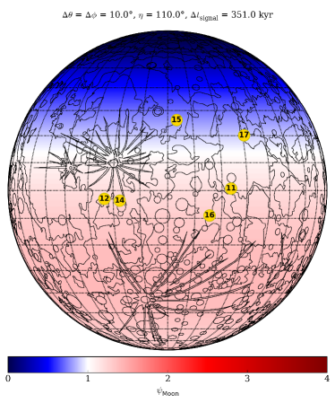
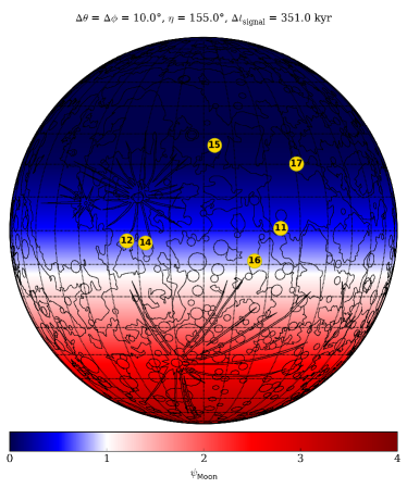
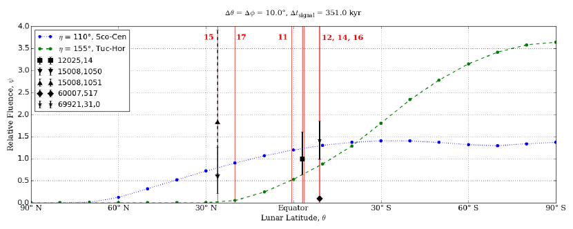
Figure 5.— Sample predicted values for the lunar distribution factor, $\psi_{\rm Moon}$. For SN material arriving from $\eta=110^{\circ}$, corresponding to a SN in the Sco-Cen region (top, left panel), and $\eta=155^{\circ}$, corresponding to a SN in the Tuc-Hor region (top, right panel). Apollo landing sites are highlighted by the numbered, yellow circles in the upper panels and vertical, red lines in the lower panel (Davies et al., 1987; Davies & Colvin, 2000). The Fimiani et al. (2016) measurements are shown in black; of note are the large error ranges particularly for the 15008 samples. Like Figure 3, the plotting program smooths grid-to-grid, however, the lower panel shows the latitudinally-averaged relative fluences for the top panels. The actual model averages are shown with data points, and the connecting lines show a smooth, nearly sine-function profile. The lunar background diagram used with permission from Steven Dutch, University of Wisconsin at Green Bay.

5.2. Lunar ${}^{60}{\rm Fe}$ Distribution

In contrast to the Earth, the airless and dessicated Moon will introduce none of the atmospheric and oceanic transport effects that influence the terrestrial ${}^{60}{\rm Fe}$ deposition on the ocean floor. In particular, lunar deposition of SN debris will not suffer the large smearing over latitudes that plague material passing through the Earth’s MLT. Consequently, the lunar distribution of SN debris holds to hope of retaining information about the SN direction.

Like Earth’s upper atmosphere, dust grains impacting the lunar surface would be deflected $\lesssim 1^{\circ}$ from their passage through the Solar System, but the lunar deposits would not be further shifted by wind/water. Because atmospheric and ocean effects can be ignored, the SN directionality will be preserved. We can adapt the method for finding upper atmosphere deposition (§4.2 and Appendix A) by using lunar parameters (daily period: 27 days, precessional period: 19 years, inclination angle: 6.7^∘). The deposition forms a banded pattern like that shown in Figure 5. We again see that the distribution is uniform across longitudes due to lunar rotation, but a latitude gradient persists and reflects the SN’s direction, smeared somewhat by precession. The upper left panel (Figure 5) assumes $\eta=110^{\circ}$, corresponding to a SN in the Sco-Cen region, and the upper right panel (Figure 5) is based on a source with $\eta=155^{\circ}$, corresponding to a SN in the Tuc-Hor region.

Fimiani et al. (2016) recently published measurements of lunar ${}^{60}{\rm Fe}$ collected during the Apollo Moon landings. The measurements cover a range of depths, but an impactor will only penetrate to a depth on order with its diameter ($\sim\mu$m for our SN grains), so we compare only the fluences of the shallowest samples (this will allow for some minor gardening as noted by Fimiani et al., 2016, and references therein). We calculated fluences as outlined in §3.2, adjusted for 10% cosmogenic (i.e., cosmic ray-produced) ${}^{60}{\rm Fe}$, and plotted the results against the expected Sco-Cen and Tuc-Hor relative fluences in Figure 5. Since we do not know the actual fluence for an isotropic distribution on the Moon, we scaled the fluences to the 12025,14 sample fluence. We see that it is not yet possible to differentiate between a Sco-Cen or Tuc-Hor source because the samples were drawn near the lunar equator and the large uncertainties in the measurements (we also note that a future, more detailed examination should address the effects of regolith composition, gardening, and impactor penetration depth). The uncertainties are the result of low-number statistics (the two plotted 15008 values are from a total of four events, see Fimiani et al., 2016, Supplemental Information), but continued study will further refine these values.

6. Conclusions

After examining the major influences on SN material as it passes through the Solar System to the bottom of the ocean, we find that previous works’ assumption of an isotropic terrestrial distribution of SN material was rather naïve but, based on our results, this assumption nevertheless yields calculated distances within an order of magnitude of a full calculation incorporating a distribution factor. The dominant influence on the final distribution of SN material deposited on the Earth is the atmosphere, specifically the MLT region, due to strong zonal and meridional winds. This means that the suggestion by Fry et al. (2015) that the direction of arrival is the dominant cause of differing fluence measurements is incorrect. Whilst the angle of arrival of SN material can have drastic effects on the SN material’s initial distribution in the upper atmosphere, these variations are completely masked as the material descends to the surface.

However, although the method outlined in §4.2 may not be applicable to finding the final distribution on Earth, ${}^{60}{\rm Fe}$ measurements using lunar regolith could apply the method. We indeed find that the lunar distribution of ${}^{60}{\rm Fe}$ retains information about the SN direction. Namely, lunar rotation and precession average over longitudes but preserve a latitude gradient that peaks near the SN latitude. The recent exciting detections of ${}^{60}{\rm Fe}$ from Apollo soil core samples show a proof of principle that the Moon can act as a telescope pointing to the SN. As yet the data, clustered at the lunar equator, are too uncertain to cleanly discriminate the two putative star cluster origins (Sco-Cen versus Tuc-Hor), but future measurements – or ideally, a sample return mission from high and low lunar latitudes – could identify one possibility.

Clearly there are a number of uncertainties and assumptions included in our examination. The fluence ratios have large error uncertainties ($\sim$50%) or are simply upper limits. This is a by-product of the counting statistics in making the ${}^{60}{\rm Fe}$/Fe measurements, and future ${}^{60}{\rm Fe}$ measurements will better constrain these values. The uncertainty in the value of $U_{\rm crust}$ further complicates the fluence ratios and, whilst most likely $U_{\rm crust}\in[0.1,\ 1]$, the use of sediment samples would be preferable since $U_{\rm sediment}\approx 1$ is much more certain. Lastly, the application of Moore & Braucher’s updated BEC model to our SN ${}^{60}{\rm Fe}$ ocean transport has some limitations. Although it includes many of the relevant considerations outlined in §4.4, it focuses on aeolian dust sources of iron rather than meteoric sources, which have a different starting distribution. Additionally, the updated BEC simulations match observations better than the previous model, but still rely on observations primarily from the northern Pacific Ocean (Moore & Braucher, 2008) and underestimate the deep ocean iron concentrations. Also, we used a general conveyor belt assumption of the movement of iron in Moore & Braucher’s results, rather than following tracer particles to understand better any possible dilutions or concentrations. Because generating an ocean model to track our SN ${}^{60}{\rm Fe}$ material as it descends in the oceans with all the relevant factors described above is beyond the scope of this paper, we attribute any deviations from our observed fluence ratios and our predictions to errors in modeling iron transport within the oceans.

Based on our results, we can duplicate the observed fluence ratios. The predictions for the Medium case show good agreement with observations of all ratios. In the case of the ${\cal F}_{\rm Feige}/{\cal F}_{\rm Knie}$ ratio, the High and Low uptake values give ratios outside the error ranges and a factor $\sim$3 from the mean value. In addition, comparing the Feige (2014) and Wallner et al. (2016) calculation of $U_{\rm crust}\in[0.7,0.17]$ assuming $\psi=1$, we find good agreement with our Medium case and our calculated distribution factors. Revisiting Equation (4), for Feige (2014)/Wallner et al. (2016):

$$\frac{{\cal F}_{\rm Knie}}{{\cal F}_{\rm Feige}}=\frac{U_{\rm Knie}\psi_{\rm Knie}}{U_{\rm Feige}\psi_{\rm Feige}}=\frac{0.1\cdot 1}{1\cdot 1}=0.1\,,$$ (14)

and for this work:

$$\frac{{\cal F}_{\rm Knie}}{{\cal F}_{\rm Feige}}=\frac{0.5\cdot 0.43}{1\cdot 1.4}=0.15\in[0.7,0.17]\,.$$ (15)

Although it would be preferable to compare a sediment and crust sample drawn from the same place in the ocean to directly measure the crust uptake, this suggests that the Feige (2014); Wallner et al. (2016) $U_{\rm crust}$ values inherently include the distribution factors between sampling locations.

Moreover, using Equation (1), we see that changing the uptake also changes the calculated distance to the source for a given observed fluence; increasing the uptake $U$ increases the estimated distance, $D$, and conversely decreasing $U$ decreases $D$. If we assume that the SN that produced the measured ${}^{60}{\rm Fe}$ occurred in a stellar group (as opposed to being the explosion of an isolated star), we can compare the distances implied by each of our cases and the locations of the two candidate groups Sco-Cen and Tuc-Hor. Adapting the conditions outlined in Fry et al. (2015) to include the distribution factor, $\psi$, we find for an ECSN, in the Medium Uptake case, the implied distance is: $D=46_{-6}^{+10}$ pc, which is consistent with the distance to Tuc-Hor ($\lesssim 60$ pc) but not with Sco-Cen ($\sim$130 pc). Table 5 summarizes the implied distances for our uptake cases.

Table 5Implied Source Distances for Each Uptake Case

Case	High	Medium	Low
$\psi_{\rm Knie}=0.43$	$U_{\rm crust}=1.0$	$U_{\rm crust}=0.5$	$U_{\rm crust}=0.1$
$8-10$-$M_{\odot}$ ECSN	$45_{-6}^{+10}$ pc	$46_{-6}^{+10}$ pc	$35_{-5}^{+8}$ pc
15-$M_{\odot}$ CCSN	$61_{-8}^{+14}$ pc	$64_{-8}^{+14}$ pc	$47_{-6}^{+11}$ pc
9-$M_{\odot}$ SAGB	$82_{-8}^{+13}$ pc	$84_{-8}^{+13}$ pc	$67_{-7}^{+11}$ pc

Finally, with regards to the number of SNe producing the ${}^{60}{\rm Fe}$ signal, we find no process within the Solar System that could spread the deposition of a single SN signal to appear like that found by Wallner et al. (2016). Such a process would need to allow concentrated ${}^{60}{\rm Fe}$ to pass fairly undisturbed, but delay diluted ${}^{60}{\rm Fe}$. The only process to make such a distinction is ocean cycling, where the residence time for iron decreases when there is an overabundance of iron (§4.4), however, the delay is only $\sim 100$ years not the $\gtrsim 100~{}{\rm kyr}$ required to reproduce the Wallner et al. (2016) measurements. In addition, $\mbox{${}^{60}{\rm Fe}$}/{\rm Fe}\lesssim 10^{-14}$ in the ocean, so any ${}^{60}{\rm Fe}$ of SN origin would have no appreciable effect on ocean iron abundance. This suggests either there were multiple SNe as postulated by Breitschwerdt et al. (2016) and Wallner et al. (2016) or another process within the ISM or SN remnant is responsible for spreading the signal.

Appendix A A. Coordinate Transformations for Calculating Fluence onto a Sector

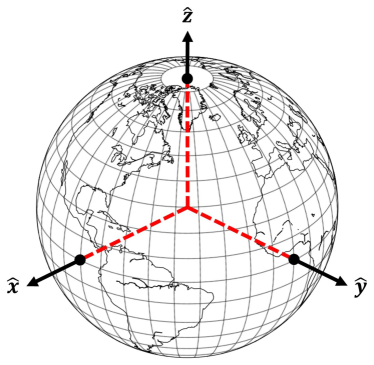
Figure 6.— Definition of terrestrial axes used in §4.2. The $+x$-axis passes through the equator at the 90^∘ W-meridian, the $+y$-axis passes through the equator at the 0^∘ meridian, and the $+z$-axis passes through the geographic North Pole.

We define the Earth’s terrestrial frame with the $+x$-axis passing through the equator at the 90^∘ W-meridian, the $+y$-axis passing through the equator at the 0^∘ meridian, and the $+z$-axis passing through the North Pole, as shown in Figure 6). We define spherical coordinates with $\theta$ as the polar angle from the $+z$-axis, $\phi$ as the azimuthal angle from the $+x$-axis, and $r$ as the radial distance from the center of the Earth:

$$\begin{pmatrix}x\\ y\\ z\end{pmatrix}=\begin{pmatrix}r\sin\theta\cos⁡\phi\\ r\sin⁡\theta\sin⁡\phi\\ r\cos⁡\theta\end{pmatrix}\,.$$ (A1)

We transform the terrestrial frame to Earth’s rotating frame (^′) by rotating about the $z$-axis with an angular speed of $\omega=7.3\times 10^{-5}$ rad s^-1 ($360^{\circ}/1\ {\rm day}$), see Figure 7:

$$\begin{pmatrix}x^{\prime}\\ y^{\prime}\\ z^{\prime}\end{pmatrix}=\begin{pmatrix}\cos\omega t&-\sin\omega t&0\\ \sin\omega t&\cos\omega t&0\\ 0&0&1\end{pmatrix}\begin{pmatrix}x\\ y\\ z\end{pmatrix}\,.$$ (A2)

Next we transform to the inclination frame (^′′) by rotating about the $x^{\prime}$-axis by an angle $\alpha=23.3^{\circ}$, see Figure 7:

$$\begin{pmatrix}x^{\prime\prime}\\ y^{\prime\prime}\\ z^{\prime\prime}\end{pmatrix}=\begin{pmatrix}1&0&0\\ 0&\cos\alpha&\sin\alpha\\ 0&-\sin\alpha&\cos\alpha\end{pmatrix}\begin{pmatrix}x^{\prime}\\ y^{\prime}\\ z^{\prime}\end{pmatrix}\,.$$ (A3)

The next transformation is to the precessing/Ecliptic frame (^′′′) by rotating about the $z^{\prime\prime}$-axis with an angular speed of $\chi=7.7\times 10^{-12}$ rad s^-1 ($360^{\circ}/26\ {\rm kyr}$), see Figure 7:

$$\begin{pmatrix}x^{\prime\prime\prime}\\ y^{\prime\prime\prime}\\ z^{\prime\prime\prime}\end{pmatrix}=\begin{pmatrix}\cos\chi t&\sin\chi t&0\\ -\sin\chi t&\cos\chi t&0\\ 0&0&1\end{pmatrix}\begin{pmatrix}x^{\prime\prime}\\ y^{\prime\prime}\\ z^{\prime\prime}\end{pmatrix}\,.$$ (A4)

Finally, we transform to the shock wave/interstellar frame (^′′′′) by rotating about the $x^{\prime\prime\prime}$-axis by an angle $\eta$ to account for different directions of arrival, see Figure 7:

$$\begin{pmatrix}x^{\prime\prime\prime\prime}\\ y^{\prime\prime\prime\prime}\\ z^{\prime\prime\prime\prime}\end{pmatrix}=\begin{pmatrix}1&0&0\\ 0&\cos\eta&-\sin\eta\\ 0&\sin\eta&\cos\eta\end{pmatrix}\begin{pmatrix}x^{\prime\prime\prime}\\ y^{\prime\prime\prime}\\ z^{\prime\prime\prime}\end{pmatrix}\,.$$ (A5)

The arrival angle, $\eta$, is defined as the angle from the Ecliptic North Pole to the SN source. In the interstellar frame, the particles travel along the $-\hat{z}^{\prime\prime\prime\prime}$-direction, or: $\vec{\mathbb{F}}(t)=-\mathbb{F}(t)\hat{z}^{\prime\prime\prime\prime}$. We also define spherical coordinates in the interstellar frame so that:

$$\begin{pmatrix}x^{\prime\prime\prime\prime}\\ y^{\prime\prime\prime\prime}\\ z^{\prime\prime\prime\prime}\end{pmatrix}=\begin{pmatrix}r^{\prime\prime\prime\prime}\sin\theta^{\prime\prime\prime\prime}\cos\phi^{\prime\prime\prime\prime}\\ r^{\prime\prime\prime\prime}\sin\theta^{\prime\prime\prime\prime}\sin\phi^{\prime\prime\prime\prime}\\ r^{\prime\prime\prime\prime}\cos\theta^{\prime\prime\prime\prime}\end{pmatrix}\,.$$ (A6)

Combining the transformations we have:

$$\begin{pmatrix}x^{\prime\prime\prime\prime}\\ y^{\prime\prime\prime\prime}\\ z^{\prime\prime\prime\prime}\end{pmatrix}=\begin{pmatrix}1&0&0\\ 0&\cos\eta&-\sin\eta\\ 0&\sin\eta&\cos\eta\end{pmatrix}\begin{pmatrix}\cos\chi t&\sin\chi t&0\\ -\sin\chi t&\cos\chi t&0\\ 0&0&1\end{pmatrix}\begin{pmatrix}1&0&0\\ 0&\cos\alpha&\sin\alpha\\ 0&-\sin\alpha&\cos\alpha\end{pmatrix}\begin{pmatrix}\cos\omega t&-\sin\omega t&0\\ \sin\omega t&\cos\omega t&0\\ 0&0&1\end{pmatrix}\begin{pmatrix}r\sin\theta\cos\phi\\ r\sin\theta\sin\phi\\ r\cos\theta\end{pmatrix}\,.$$ (A7)

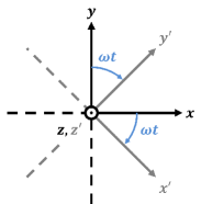
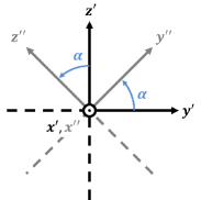
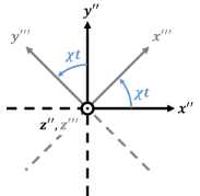
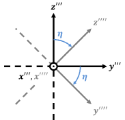
Figure 7.— Coordinate Transformations: (a) Terrestrial (unprimed) to Daily Rotation (^′), (b) Daily Rotation (^′) to Inclination (^′′), (c) Inclination (^′′) to Precessing/Ecliptic (^′′′), (d) Precessing/Ecliptic (^′′′) to Shock Wave/Interstellar (^′′′′).

With regards to the coordinate differentials, all of the coordinate transformations are rotations, which means they are special affine transformations and therefore are area- and volume-preserving. More specifically, examining the terrestrial-to-rotating frame transformation, the differential volumes are:

$$dV=d\vec{z}\cdot(d\vec{x}\times d\vec{y})=dx~{}dy~{}dz\,{\rm,and\ }dV^{\prime}=d\vec{z^{\prime}}\cdot(d\vec{x^{\prime}}\times d\vec{y^{\prime}})=dx^{\prime}~{}dy^{\prime}~{}dz^{\prime}\,,$$ (A8)

and the two sets of differentials are related according to Equation (A2):

$$d\vec{x^{\prime}} =d\vec{x}\cos\omega t-d\vec{y}\sin\omega t$$

$$d\vec{y^{\prime}} =d\vec{x}\sin\omega t+d\vec{y}\cos\omega t$$

$$d\vec{z^{\prime}} =d\vec{z}\,.$$ (A9)

Combining Equations (A8) and (A9), we get:

$$dV^{\prime} =d\vec{z^{\prime}}\cdot(d\vec{x^{\prime}}\times d\vec{y^{\prime}})=d\vec{z}\cdot\left[\left(d\vec{x}\cos\omega t-d\vec{y}\sin\omega t\right)\times\left(d\vec{x}\sin\omega t+d\vec{y}\cos\omega t\right)\right]$$

$$=d\vec{z}\cdot\left[\left(\cos^{2}\omega t+\sin^{2}\omega t\right)d\vec{x}\times d\vec{y}\right]=d\vec{z}\cdot\left[\left(1\right)d\vec{x}\times d\vec{y}\right]=d\vec{z}\cdot\left(d\vec{x}\times d\vec{y}\right)=dV$$

$$\Rightarrow dx^{\prime}~{}dy^{\prime}~{}dz^{\prime} =dx~{}dy~{}dz\,.$$ (A10)

Similar derivations can be done for the each of the other transformations, and we find:

$$\Rightarrow dx~{}dy~{}dz=dx^{\prime\prime\prime\prime}~{}dy^{\prime\prime\prime\prime}~{}dz^{\prime\prime\prime\prime}=r^{2}\sin\theta~{}d\theta~{}d\phi~{}dr=(r^{\prime\prime\prime\prime})^{2}\sin\theta^{\prime\prime\prime\prime}~{}d\theta^{\prime\prime\prime\prime}~{}d\phi^{\prime\prime\prime\prime}~{}dr^{\prime\prime\prime\prime}\,.$$ (A11)

Because there is no variation in radius, $\sin\theta~{}d\theta~{}d\phi=\sin\theta^{\prime\prime\prime\prime}~{}d\theta^{\prime\prime\prime\prime}~{}d\phi^{\prime\prime\prime\prime}\Rightarrow d\Omega=d\Omega^{\prime\prime\prime\prime}$, and $d\vec{\Omega}$ is directed away from Earth’s center. To calculate the fluence, ${\cal F}$, received by a sector of Earth, we integrate over the area of the sector:

$$dN=\vec{\mathbb{F}}(t)\cdot d\vec{A}~{}dt\Rightarrow\frac{dN}{A}=\frac{\vec{\mathbb{F}}(t)\cdot d\vec{A}~{}dt}{A},d\vec{A}=r^{2}d\vec{\Omega}$$ (A12)

$$\Rightarrow d{\cal F}=\frac{\vec{\mathbb{F}}(t)\cdot r^{2}d\vec{\Omega}~{}dt}{r^{2}\Omega}=\frac{\vec{\mathbb{F}}(t)\cdot d\vec{\Omega}~{}dt}{\Omega}$$ (A13)

$$\Rightarrow{\cal F}=\frac{\iiint\vec{\mathbb{F}}(t)\cdot d\vec{\Omega}~{}dt}{\Omega},\mathbb{F}(t)=\mathbb{F}_{0}\left(1-\frac{t}{\Delta t_{\rm signal}}\right)\,.$$ (A14)

In the interstellar frame, $\theta^{\prime\prime\prime\prime}$ and $\phi^{\prime\prime\prime\prime}$ do not depend on time, $t$:

$${\cal F}=\frac{\iiint\vec{\mathbb{F}}(t)\cdot d\vec{\Omega}^{\prime\prime\prime\prime}dt}{\Omega}=\frac{1}{\Omega}\iiint-\mathbb{F}(t)\cos\left(\pi-\theta^{\prime\prime\prime\prime}\right)d\Omega^{\prime\prime\prime\prime}dt=\frac{1}{\Omega}\iiint\mathbb{F}(t)\cos\theta^{\prime\prime\prime\prime}d\Omega^{\prime\prime\prime\prime}dt$$ (A15)

$$\Rightarrow{\cal F}=\frac{1}{\Omega}\int_{t_{\rm ini}}^{t_{\rm fin}}\mathbb{F}(t)dt\iint_{S}\cos\theta^{\prime\prime\prime\prime}\sin\theta^{\prime\prime\prime\prime}d\theta^{\prime\prime\prime\prime}d\phi^{\prime\prime\prime\prime}$$ (A16)

The first integral is straightforward:

$$\int_{t_{\rm ini}}^{t_{\rm fin}}\mathbb{F}(t)dt=\mathbb{F}_{0}\left[t-\frac{t^{2}}{2\Delta t_{\rm signal}}\right]_{t_{\rm ini}}^{t_{\rm fin}}=\mathbb{F}_{0}\left(\frac{t_{\rm ini}^{2}-t_{\rm fin}^{2}}{2\Delta t_{\rm signal}}+t_{\rm fin}-t_{\rm ini}\right)\,,$$ (A17)

and the second integral is the projected area of a spherical sector onto the $x^{\prime\prime\prime\prime}-y^{\prime\prime\prime\prime}$-plane, see Figure 8.

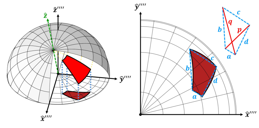
Figure 8.— Sector area approximation. The area of the projection of the sector onto the $x^{\prime\prime\prime\prime}-y^{\prime\prime\prime\prime}$-plane is approximated using Bretschneider’s Formula for 4-sided sectors and Heron’s Formula for 3-sided sectors.

Because the SN dust particles are traveling in the $-\hat{z}^{\prime\prime\prime\prime}$-direction by construction, the surface integral in Equation (A16) represents the area of the sector projected onto the $x^{\prime\prime\prime\prime}-y^{\prime\prime\prime\prime}$-plane (see Figure 8). While it is fairly straightforward to transform the sector vertices from the terrestrial to the interstellar frame (e.g., $\theta_{u}\rightarrow\theta_{u}^{\prime\prime\prime\prime}$, etc.) the path from each vertex is not, requiring a dependence on $\phi^{\prime\prime\prime\prime}$ in the limits of integration for $\theta^{\prime\prime\prime\prime}$ (or vice versa):

$$\iint_{S}\cos\theta^{\prime\prime\prime\prime}\sin\theta^{\prime\prime\prime\prime}d\theta^{\prime\prime\prime\prime}d\phi^{\prime\prime\prime\prime}=\int_{\phi_{l}^{\prime\prime\prime\prime}}^{\phi_{u}^{\prime\prime\prime\prime}}\int_{g(\phi^{\prime\prime\prime\prime})}^{f(\phi^{\prime\prime\prime\prime})}\cos\theta^{\prime\prime\prime\prime}\sin\theta^{\prime\prime\prime\prime}d\theta^{\prime\prime\prime\prime}d\phi^{\prime\prime\prime\prime}\,,$$ (A18)

where $f$ and $g$ are the transformed paths between vertices. In order to simplify our calculations, rather than derive the transformation functions, we approximate the area of the projection (and the integral) as a general quadrilateral (or triangle in the case where $\theta_{l}=0^{\circ}$ or $\theta_{u}=180^{\circ}$). In other words:

$$\iint_{S}\cos\theta^{\prime\prime\prime\prime}\sin\theta^{\prime\prime\prime\prime}d\theta^{\prime\prime\prime\prime}d\phi^{\prime\prime\prime\prime}\approx\begin{cases}\sqrt{s(s-a)(s-b)(s-c)}&\quad\text{if }\theta_{l}=0^{\circ}\text{ or }\theta_{u}=180^{\circ}\,,\\ \\ \frac{1}{4}\sqrt{4~{}p^{2}~{}q^{2}-\left(b^{2}+d^{2}-a^{2}-c^{2}\right)^{2}}&\quad\text{otherwise}\,,\\ \end{cases}$$ (A19)

where $a$, $b$, $c$ and $d$ are the lengths of each side, $p$ and $q$ are the lengths of the diagonals of the quadrilateral, and $s$ is the semi-perimeter of the triangle ($s\equiv(a+b+c)/2$).

For a given latitude and longitude $(\theta,\phi)$ and gridsize $(\Delta\theta\times\Delta\phi)$, these correspond to grid boundaries at: $\theta_{l}=\theta-\Delta\theta/2$, $\theta_{u}=\theta+\Delta\theta/2$, $\phi_{l}=\phi-\Delta\phi/2$, and $\phi_{u}=\phi+\Delta\phi/2$. Using Equation (A7) and setting $r=1\ R_{\oplus}$, we transform the grid vertices to their associated $(x^{\prime\prime\prime\prime},y^{\prime\prime\prime\prime},z^{\prime\prime\prime\prime})$ coordinates. The distances between the $(x^{\prime\prime\prime\prime},y^{\prime\prime\prime\prime},0)$ coordinates are used to find the associated $a$, $b$, $c$, $d$, $p$, and $q$ values. For our particular approach, the vertices correspond to:

$$a~{} \widehat{=}~{}\overline{\left(\phi_{l},\theta_{l}\right)\left(\phi_{u},\theta_{l}\right)} b~{} \widehat{=}~{}\overline{\left(\phi_{u},\theta_{l}\right)\left(\phi_{u},\theta_{u}\right)} c~{} \widehat{=}~{}\overline{\left(\phi_{u},\theta_{u}\right)\left(\phi_{l},\theta_{u}\right)}$$

$$d~{} \widehat{=}~{}\overline{\left(\phi_{l},\theta_{u}\right)\left(\phi_{l},\theta_{l}\right)} p~{} \widehat{=}~{}\overline{\left(\phi_{u},\theta_{l}\right)\left(\phi_{l},\theta_{u}\right)} q~{} \widehat{=}~{}\overline{\left(\phi_{l},\theta_{l}\right)\left(\phi_{u},\theta_{u}\right)}\,.$$ (A20)

If any of the $z^{\prime\prime\prime\prime}$ values for the vertices are negative, corresponding to the sector being on the opposite side of the Earth from the arriving flux, the area of the sector is zero. This increases the error in our approximation along the edges, but our time intervals are such that the errors are consistent across the entire surface, and we are interested in the relative values across the globe.

Finally, to calculate the fluences for each of the sectors (for $\Delta\theta=\Delta\phi=10^{\circ}$ there are 648 sectors), we calculate the fluence received at each time step on each sector then sum over all time steps for each sector (presumably the time steps cover the entire duration of the SN signal, although after one precessional cycle the final pattern changes very little). We use Equation (A17) to find the fluence incident to the sector during that time step (given by Equations (12) and (13)), and we use Equation (A19) to find the cross-sectional area facing the incident SN dust flux. The product of these two values gives the sector fluence at each time step. Once the sector fluence has been summed over all time steps (the result of Equation (A16)), the value of $\psi$ for each sector is found by scaling the total sector fluence by the total area-weighted average fluence of the entire sphere. For our chosen grid size of $\Delta\theta=\Delta\phi=10^{\circ}$, this approximation is accurate to $\lesssim 1\%$, and for our results in Figures 3 and 5, this approximation demonstrated convergence to the precision given.

Appendix B B. Heliosphere IMF Model

We use the model outlined in Parker (1958) and Gustafson (1994). Using a right-handed, spherical coordinate system with the Sun at the origin, we define $\phi$ as the azimuthal angle along the Sun’s equator and $\theta$ as the angle from the Sun’s rotational axis. Because of the Sun’s rotation and a magnetic field frozen-in the radially expanding solar wind, the components of the IMF take the form:

$$B_{r} =B_{r,0}\left(\frac{r_{0}}{r}\right)^{2}{\rm sgn}\left(\pi/2-\theta\right)\,,$$ (B1)

$$B_{\theta} =0\,,$$ (B2)

$$B_{\phi} =B_{\phi,0}\left(\frac{r_{0}}{r}\right)\sin{\theta}~{}{\rm sgn}\left(\pi/2-\theta\right)\,,$$ (B3)

where $B_{r,0}$ and $B_{\phi,0}$ are the magnetic field components at $r_{0}$ and ${\rm sgn}\left(\pi/2-\theta\right)$ accounts for the different polarities in the northern and southern solar hemispheres. From Gustafson (1994), for $r_{0}=1$ AU, $B_{r,0}\approx B_{\phi,0}\approx 30\ \mu$G.

Appendix C C. Earth’s Magnetosphere Model

The Katsiaris & Psillakis (1987) Magnetosphere model defines its right-handed axes with the origin at the Earth, the $\hat{X}$-axis towards the Sun, the $\hat{Z}$-axis through the geographic North, and takes the form:

$$\vec{B}=\vec{B}_{\rm dipole}+\vec{B}_{\rm tail}\,,$$ (C1)

with:

$$\vec{B}_{\rm dipole}=-\frac{3MZX}{R^{5}}\hat{X}-\frac{3MZY}{R^{5}}\hat{Y}+\left(\frac{M}{R_{3}}-\frac{3MZ^{2}}{R^{5}}\right)\hat{Z}\,,$$ (C2)

$$\vec{B}_{\rm tail}=\left(B_{X0}\tanh\left(Z/H\right)\right)\hat{X}-B_{Z0}\hat{Z}\,,$$ (C3)

and

$$R^{2}=X^{2}+Y^{2}+Z^{2}\,,$$ (C4)

where $M$ is the magnetic dipole strength based on the surface value, and $B_{Z0}$ is a uniform magnetic field normal to the dipole’s equatorial plane.

References

- Adams et al. (2013) Adams, S. M., Kochanek, C. S., Beacom, J. F., Vagins, M. R., & Stanek, K. Z. 2013, ApJ, 778, 164
- Alvarez et al. (1980) Alvarez, L., Alvarez, W., Asaro, F., & Michel, H. 1980, Sci, 208, 4448, 1095-1108
- Archer & Johnson (2000) Archer, D. E., & Johnson, K. 2000, Global Biogeochemical Cycles, 14, 269
- Athanassiadou & Fields (2011) Athanassiadou, T. & Fields, B. D. 2011, New Astron., 16, 4, 229-241
- Benítez et al. (2002) Benítez, N., Maíz-Apellániz, J., & Canelles, M. 2002, Physical Review Letters, 88, 081101
- Bishop & Egli (2011) Bishop, S. & Egli, R. 2011, Icarus, 212, 2, 960-962
- Boyd & Ellwood (2010) Boyd, P. W., & Ellwood, M. J. 2010, Nature Geoscience, 3, 675
- Breitschwerdt et al. (2012) Breitschwerdt, D., de Avillez, M. A., Feige, J., & Dettbarn, C. 2012, Astronomische Nachrichten, 333, 486
- Breitschwerdt et al. (2016) Breitschwerdt, D., Feige, J., Schulreich, M. M., et al. 2016, Nature, 532, 73
- Bruland et al. (1994) Bruland, K. W., Orians, K. J., & Cowen, J. P. 1994, Geochim. Cosmochim. Acta, 58, 3171
- Chmeleff et al. (2010) Chmeleff, J., von Blanckenburg, F., Kossert, K., & Jakob, D. 2010, Nuclear Instruments and Methods in Physics Research B, 268, 192
- Cook et al. (2009) Cook, D. L., Berger, E., Faestermann, T., et al. 2009, LPI, 40, 1129
- Croot et al. (2004) Croot, P. L., Streu, P., & Baker, A. R. 2004, Geophys. Res. Lett., 31, L23S08
- Davies et al. (1987) Davies, M. E., Colvin, T. R., & Meyer, D. L. 1987, J. Geophys. Res., 92, 14177
- Davies & Colvin (2000) Davies, M. E., & Colvin, T. R. 2000, J. Geophys. Res., 105, 20277
- Dhomse et al. (2013) Dhomse, S. S., Saunders, R. W., Tian, W., Chipperfield, M. P., & Plane, J. M. C. 2013, Geophys. Res. Lett., 40, 4454
- Dragt (1965) Dragt, A. J. 1965, Reviews of Geophysics and Space Physics, 3, 255
- Dutkiewicz et al. (2005) Dutkiewicz, S., Follows, M. J., & Parekh, P. 2005, Global Biogeochemical Cycles, 19, GB1021
- Dutkiewicz et al. (2012) Dutkiewicz, S., Ward, B. A., Monteiro, F., & Follows, M. J. 2012, Global Biogeochemical Cycles, 26, GB1012
- Ellis & Schramm (1995) Ellis, J., & Schramm, D. N. 1995, Proceedings of the National Academy of Science, 92, 235
- Ellis et al. (1996) Ellis, J., Fields, B. D., & Schramm, D. N. 1996, ApJ, 470, 1227
- Feige et al. (2012) Feige, J., Wallner, A., Winkler, S. R., et al. 2012, PASA, 29, 2, 109-114
- Feige et al. (2013) Feige, J., Wallner, A., Fifield, L. K., et al. 2013, EPJWC, 63, 03003
- Feige (2014) Feige, J. “Supernova-Produced Radionuclides in Deep-Sea Sediments Measured with AMS.” Doctoral Dissertation, University of Vienna, 2014. http://othes.univie.ac.at/35089/
- Feng et al. (2013) Feng, W., Marsh, D. R., Chipperfield, M. P., et al. 2013, Journal of Geophysical Research (Atmospheres), 118, 9456
- Fields et al. (2008) Fields, B. D., Athanassiadou, T., & Johnson, S. R. 2008, ApJ, 678, 1, 549-562
- Fimiani et al. (2012) Fimiani, L., Cook, D. L., Faestermann, T., et al. 2012, LPI, 43, 1279
- Fimiani et al. (2014) Fimiani, L., Cook, D. L., Faestermann, T., et al. 2014, LPI, 45, 1778
- Fimiani et al. (2016) Fimiani, L., Cook, D. L., Faestermann, T., et al. 2016, Physical Review Letters, 116, 151104
- Fitoussi et al. (2008) Fitoussi, C., Raisbeck, G. M., Knie, K., et al. 2008, PhRvL., 101, 12, 121101
- Fry et al. (2015) Fry, B. J., Fields, B. D., & Ellis, J. R. 2015, ApJ, 800, 71
- Fuchs et al. (2006) Fuchs, B., Breitschwerdt, D., de Avillez, M. A., Dettbarn, C., & Flynn, C. 2006, MNRAS, 373, 3, 993-1003
- Gustafson (1994) Gustafson, B.A.S. 1994, Annual Review of Earth and Planetary Sciences, 22, 553
- Jickells et al. (2005) Jickells, T. D., An, Z. S., Andersen, K. K., et al. 2005, Science, 308, 67
- Binns et al. (2016) Binns, W. R., Israel, M. H., Christian, E. R., et al. 2016, Science, 352, 677
- Kachelrieß et al. (2015) Kachelrieß, M., Neronov, A., & Semikoz, D. V. 2015, Physical Review Letters, 115, 181103
- Katsiaris & Psillakis (1987) Katsiaris, G. A., & Psillakis, Z. M. 1987, Ap&SS, 132, 165
- Kimura & Mann (1998) Kimura, H., & Mann, I. 1998, ApJ, 499, 454
- Kivelson & Russell (1995) Kivelson, M. G., & Russell, C. T. 1995, Introduction to Space Physics, Edited by Margaret G. Kivelson and Christopher T. Russell, pp. 586. ISBN 0521451043. Cambridge, UK: Cambridge University Press, April 1995.,
- Knie et al. (1999) Knie, K., Korschinek, G., Faestermann, T., et al. 1999, PhRvL, 83, 1, 18-21
- Knie et al. (2004) Knie, K., Korschinek, G., Faestermann, T., et al. 2004, PhRvL, 93, 17, 171103
- Korschinek et al. (1996) Korschinek, G., Faestermann, T., Knie, K. & Schmidt, C. 1996, Radiocarbon, 38, 68
- Korschinek et al. (2010) Korschinek, G., Bergmaier, A., Faestermann, T., et al. 2010, Nuclear Instruments and Methods in Physics Research B, 268, 187
- LefèVre & Watson (1999) LefèVre, N., & Watson, A. J. 1999, Global Biogeochemical Cycles, 13, 727
- Mamajek (2016) Mamajek, E. E. 2016, IAU Symposium, 314, 21
- Moore et al. (2004) Moore, J. K., Doney, S. C., & Lindsay, K. 2004, Global Biogeochemical Cycles, 18, GB4028
- Moore & Braucher (2008) Moore, J. K., & Braucher, O. 2008, Biogeosciences, 5, 631
- Murray et al. (2004) Murray, N., Weingartner, J.C., & Capobianco, C. 2004, ApJ, 600, 804
- Niciejewski et al. (2011) Niciejewski, R., Skinner, W., Cooper, M., et al. 2011, Journal of Geophysical Research (Space Physics), 116, A05302
- Parekh et al. (2004) Parekh, P., Follows, M. J., & Boyle, E. 2004, Global Biogeochemical Cycles, 18, GB1002
- Parker (1958) Parker, E. N. 1958, ApJ, 128, 664
- Parker (1963) Parker, E. N. 1963, New York, Interscience Publishers, 1963.
- Plane (2012) Plane, J. M. C. 2012, Chemical Society Reviews, Vol. 41, p. 6507-6518, 2012, 41, 6507
- Plane et al. (2015) Plane, J. M. C., Feng, W., Dawkins, E. C. M. 2015, Chemical Reviews, 115(10), 4497-4541
- Rugel et al. (2009) Rugel, G., Faestermann, T., Knie, K., et al. 2009, Physical Review Letters, 103, 072502
- Saunders et al. (2012) Saunders, R. W., Dhomse, S., Tian, W. S., Chipperfield, M. P., & Plane, J. M. C. 2012, Atmospheric Chemistry & Physics, 12, 4387
- Savchenko et al. (2015) Savchenko, V., Kachelrieß, M., & Semikoz, D. V. 2015, ApJ, 809, L23
- Shklovskii (1968) Shklovskii, I. S. 1968, Supernovae, New York: Wiley
- Slavin et al. (1985) Slavin, J. A., Smith, E. J., Sibeck, D. G., Baker, D. N., & Zwickl, R. D. 1985, J. Geophys. Res., 90, 10875
- Sterken et al. (2012) Sterken, V. J., Altobelli, N., Kempf, S., et al. 2012, A&A, 538, A102
- Sterken et al. (2013) Sterken, V. J., Altobelli, N., Kempf, S., et al. 2013, A&A, 552, A130
- Tsyganenko (1989) Tsyganenko, N. A. 1989, Planet. Space Sci., 37, 5
- Wagner et al. (1979) Wagner, J. S., Kan, J. R., & Akasofu, S.-I. 1979, J. Geophys. Res., 84, 891
- Wallner et al. (2000) Wallner, C., Faestermann, T., Gerstmann, U., et al. 2000, Nuclear Instruments and Methods in Physics Research B, 172, 333
- Wallner et al. (2004) Wallner, C., Faestermann, T., Gerstmann, U., et al. 2004, New Astron. Rev., 48, 145
- Wallner et al. (2015a) Wallner, A., Faestermann, T., Feige, J., et al. 2015, Nature Communications, 6, 5956
- Wallner et al. (2015b) Wallner, A., Bichler, M., Buczak, K., et al. 2015, Physical Review Letters, 114, 041101
- Wallner et al. (2016) Wallner, A., Feige, J., Kinoshita, N., et al. 2016, Nature, 532, 69